Elements for the Successful Computer Simulation of Sediment Management Strategies for Reservoirs

Abstract

Computer simulation of reservoir sediment management strategies is becoming more important as worldwide water supply shrinks due to sediment deposition, while population growth continues. We identified the physical processes underlying each of the several alternatives available to transport incoming or deposited sediments downstream into receiving waters and the governing equations that describe each process. The purpose of this paper is to understand how physical characteristics of reservoir sediment management can be simulated with available computer codes. We described commonly available computer codes and their abilities to solve the appropriate equations in one, two, or three dimensions. The results revealed that one dimensional models are most appropriate for long-term simulations of the evolving reservoir bottom profile, while two or three dimensional codes are more appropriate for simulating density currents and detailed lateral movement of sediments, such as during local pressure flushing near reservoir outlets. We conclude that existing codes can successfully simulate sediment management, but because each code has limitations, they require seasoned judgment in their choice, application, and interpretation. Incorporating sediment prediction and management correctly into the planning, design, and operational phases of dam projects is essential for ensuring that the benefits of reservoir storage are sustained over the long term. The implications of our key findings are that sediment management strategies can be successfully simulated and that such simulations should be performed for our aging dams and newly proposed projects.

1. Introduction

The design of a reservoir project entails the determination of the required storage capacity over multiple years [1]. Reservoir storage space is a key factor for production of water and so-called renewable energy supply, and it is becoming increasingly important as water demand and climate change-related stresses increase and as suitable storage sites become scarce [2].

Within any geographic area, the rate of storage loss due to sedimentation will vary widely because of differences in soils, land cover, and land use [3]. Sediment management ultimately is site specific and most urgent at reservoirs whose storage has been dramatically reduced. For example, in Switzerland, due to low sediment inflow and repeated sediment venting, the average annual loss in reservoir capacity is only 0.2% [4], while in China, due to high sediment inflow rates, the mean annual loss rate in storage capacity is 2.3% [5]. Estimates show that about 0.5% to 1% of the total volume of global reservoir storage is lost annually [6]. This means that without further action, one quarter of all dams will lose their storage to sedimentation in the next 25 to 50 years [7], but negative upstream and downstream impacts are manifest well before all storage is lost.

Reservoirs, as a vital component of water infrastructure, are thus non-sustainable, and mitigation measures are urgently needed to increase project lifetimes [8] and switching to sustainable infrastructure. The prediction of sediment yield, deposition, and erosion associated with reservoirs is therefore critical, including simulating the various sediment management alternatives (to be discussed shortly). Although, those alternatives have the common purpose of achieving sustainable reservoir storage, better understanding the elements associated with each will enhance benefits and the effectiveness of reservoir operations. Each sediment management alternative has unique physical characteristics and simulation of these alternatives is not straightforward. The purpose of this paper is to understand how physical characteristics of sedimentation in reservoirs can be simulated with available computer codes. “Code” in this paper refers to the compiled program used to simulate sediment management scenarios. Such simulations are referred to as models. This evaluation is addressed through governing equations and explaining features of one- and multi-dimensional codes. Incorporating sediment prediction and management correctly into the planning, design, and operational phases of dam projects is essential for ensuring that the benefits of reservoir storage are sustained well into the future.

Our materials and methods are described in the next three sections where we formulate the physical processes foundational to each sediment management alternative. Understanding the dominant physical processes for each sediment management option is the first step toward an efficient simulation. Next are presented the governing equations that describe the physical processes and the commonly available computer codes for simulating them. The results follow with citations of successful simulation studies using the identified codes. Published reservoir sediment management simulation studies demonstrate which computer codes can be used for reservoir sediment simulation. Finally, the discussion section summarizes the main findings relevant for all the management alternatives and their unique features.

2. Physical Processes Associated with Sediment Management Alternatives

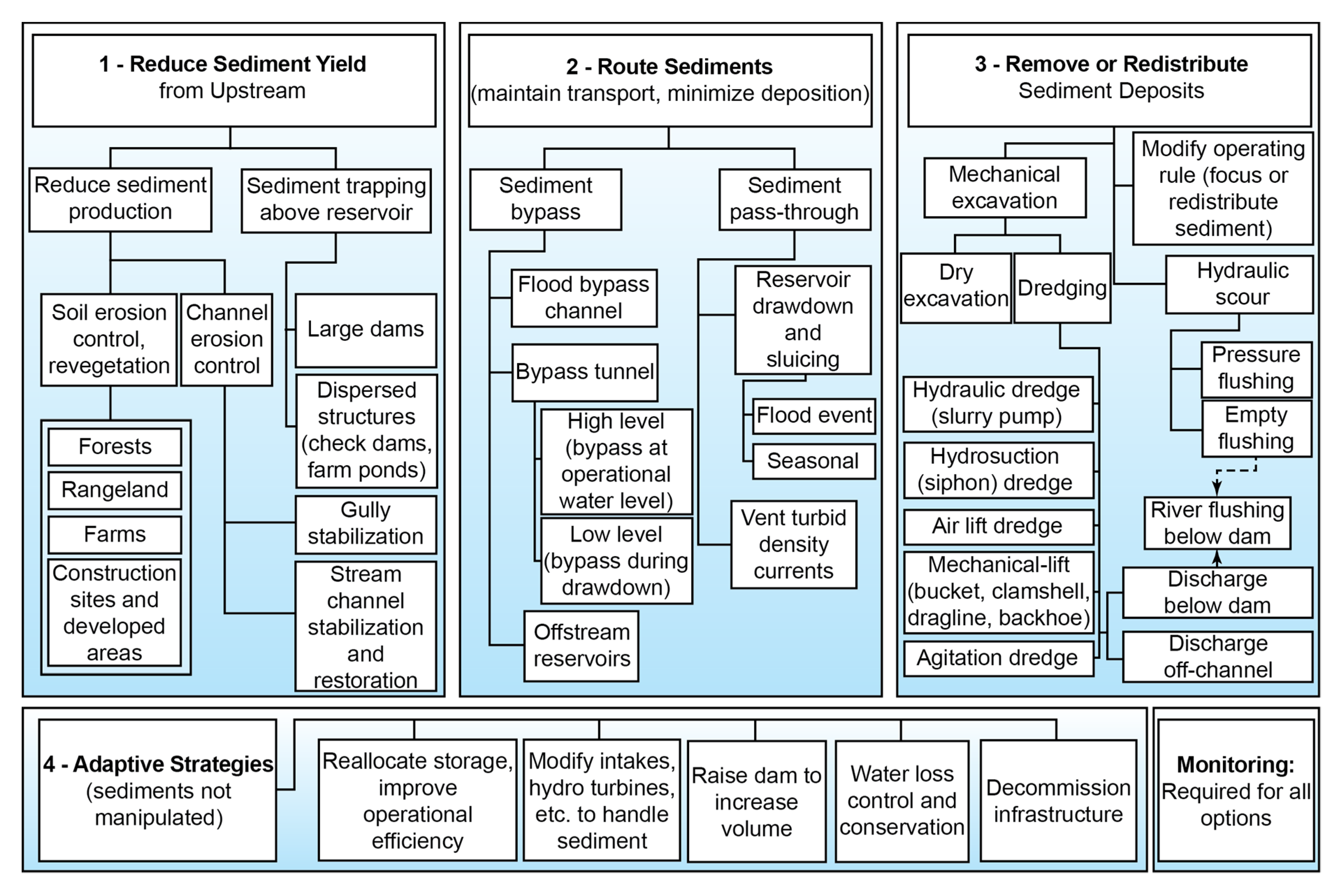
The many methods of managing reservoir sedimentation are summarized in Figure 1 and are divided into three major categories: reducing sediment yield, routing sediments, and removing or redistributing sediments [9]. The cost and applicability of each strategy is function of site geometry and the volume of sediment accumulation.

The fourth group focuses on increasing reservoir storage without manipulating sediment. However, even the largest reservoirs will eventually require sediment management or be decommissioned [3]. Monitoring shown as a separate function is crucial to track both loss and recovery of reservoir storage.

Successfully simulating reservoir sediment management strategies depends on a sound understanding of the physical processes that govern each technique. The successful simulation requires suitable and comprehensive knowledge about the alternative we want to simulate. For example, a mistake in estimating sediment inflow into a reservoir especially during flood events produces incorrect bed elevations in the reservoir and an incorrect simulation of sediment flushing [10]. Operational conditions for each alternative are also crucial. For example, according to the feasibility study carried out by Consorcio PCA (2012), the minimum outflow from a bottom outlet to achieve efficient flushing should be at least twice the annual mean flow [11].

Simulating the topographic surface to represent the bottom geometry during operation is one of the most important aspects of any reservoir model simulation. Moreover, reservoir pool elevation and configuration has a major influence on hydraulic behavior and the pattern of sediment deposition in reservoirs [3].

Although every computer code has assumptions and constraints, which impact accuracy, users must recognize the main and governing physical processes underlying sediment management techniques, so they can more successfully select the appropriate computer code to simulate the condition.

Table 1. Dominant physical processes associated with sediment management techniques.

Sediment Management Technique	Sediment Management Category and Dominant Physical Processes to be Simulated by Computer Codes
Route Sediments
Sediment bypass tunnel	Sediment distribution in water column, wear on tunnel perimeter, sediment transport in supercritical flow, splitting sediments at intake
Sediment pass-through
Drawdown and sluicing	Sediment suspension, multiple grain size sediment transport
Turbidity current	Hyper-concentrated flow, sediment entrainment and deposition, plume momentum, diffusion
Hydrosuction Sediment Removal System (HSRS)	Sediment entrainment, slurry transport in pipes, sufficient head difference
Remove Deposits
Flushing	Sediment entrainment, multiple grain size sediment transport, bank stability
Pressure flushing	Incipient motion, cohesive sediment transport
Hydraulic dredging	Sediment cohesion, slurry transport in pipes
HSRS	Sediment entrainment, slurry transport in pipes, incipient motion

presents the dominant physical processes for alternatives in Categories 2 and 3 of Figure 1, both of which emphasize transporting sediments downstream from the dam. Category 1, Reducing Sediment Yield, is beyond the scope of this paper.

A summary and brief discussion of the equations of motion for water and sediment that describe the physical processes of Table 1 is discussed next, followed by a description of codes found capable of solving such equations.

3. Equations and Computer Codes for Reservoir Sediment Management

3.1. Summary of Basic Equations

Two mathematical approaches can be used to describe water and sediment transport. One is the two-fluid model that considers water and sediment as two fluids and uses the continuity and momentum equations for each fluid. The two-fluid model is, however, quite complex [12], and will not be considered further. The other approach is the diffusion model that evaluates the transport and dispersion of sediment particles in the water column and uses the continuity and momentum equations for the sediment-laden flow and the diffusion equation for sediment grains. The flow and sediment transport equations presented here are based on the diffusion model. All variables are defined in the notation section.

3.1.1. Three-Dimensional

The equations governing bottom adjustment and the turbulent transport of a water and sediment mixture with density $\rho$ and velocity $\overrightarrow{u}=\left(u,v, w\right)$ vector in a Cartesian coordinate system ($x$, $y$, $z$) over time $t$ are given below.

Mass Conservation:

$$\frac{\partial \rho }{\partial t}+\frac{\partial \left(\rho u\right)}{\partial x}+\frac{\partial \left(\rho v\right)}{\partial y}+\frac{\partial \left(\rho w\right)}{\partial z}=0$$

(1)

Momentum Conservation:

$$\frac{\partial u}{\partial t}+\frac{\partial uu}{\partial x}+\frac{\partial uv}{\partial y}+\frac{\partial uw}{\partial z}=-\frac{1}{\rho }\frac{\partial p}{\partial x}+\frac{\partial }{\partial x}\left({\upsilon }_t\frac{\partial u}{\partial x}\right)+\frac{\partial }{\partial y}\left({\upsilon }_t\frac{\partial u}{\partial y}\right)+\frac{\partial }{\partial z}\left({\upsilon }_t\frac{\partial u}{\partial z}\right)$$

(2)

$$\frac{\partial v}{\partial t}+\frac{\partial uv}{\partial x}+\frac{\partial vv}{\partial y}+\frac{\partial vw}{\partial z}=-\frac{1}{\rho }\frac{\partial p}{\partial y}+\frac{\partial }{\partial x}\left({\upsilon }_t\frac{\partial v}{\partial x}\right)+\frac{\partial }{\partial y}\left({\upsilon }_t\frac{\partial v}{\partial y}\right)+\frac{\partial }{\partial z}\left({\upsilon }_t\frac{\partial v}{\partial z}\right)$$

(3)

$$\frac{\partial w}{\partial t}+\frac{\partial uw}{\partial x}+\frac{\partial vw}{\partial y}+\frac{\partial ww}{\partial z}=-g-\frac{1}{\rho }\frac{\partial p}{\partial z}+\frac{\partial }{\partial x}\left({\upsilon }_t\frac{\partial w}{\partial x}\right)+\frac{\partial }{\partial y}\left({\upsilon }_t\frac{\partial w}{\partial y}\right)+\frac{\partial }{\partial z}\left({\upsilon }_t\frac{\partial w}{\partial z}\right)$$

(4)

where $p$ is pressure, ${\upsilon }_t$ is eddy viscosity, and $g$ is gravitational acceleration. Note, that the gravity force is the only external body force considered in the above equation.

Sediment Advection-Diffusion Transport:

$$\frac{\partial c}{\partial t}+\frac{\partial uc}{\partial x}+\frac{\partial vc}{\partial y}+\frac{\partial wc}{\partial z}-\frac{\partial w_{f}c}{\partial z}=\frac{\partial }{\partial x}\left({ϵ}_s\frac{\partial c}{\partial x}\right)+\frac{\partial }{\partial y}\left({ϵ}_s\frac{\partial c}{\partial y}\right)+\frac{\partial }{\partial z}\left({ϵ}_s\frac{\partial c}{\partial z}\right)$$

(5)

where $c$ is volumetric sediment concentration, $w_f$ is sediment particle fall velocity, and ${ϵ}_s$ and is eddy diffusivity of sediment particles. The net flux of sediment particles between the flow and bottom ($D-E$, where $D=c_b{w}_f$ is deposition rate of sediment onto the bed, $c_b$ is the near-bed sediment concentration, $E=c_{be}{w}_f$ is entrainment rate of sediment from the bed, and $c_{be}$ is the equilibrium near-bed sediment concentration) is imposed as a boundary condition.

Bed Sediment Mass Conservation:

$$\left(1-\eta \right)\frac{\partial Z_b}{\partial t}+E-D=0$$

(6)

where $\eta$ is porosity and $Z_b$ is bottom elevation.

3.1.2. Two-Dimensional

The equations describing the transport of water and sediment in two dimensions are derived by integrating the above three-dimensional Equations (1)–(5) across the water depth $h$. Depth-averaged variables are indicated by an overbar.

Mass Conservation:

$$\frac{\partial \rho h}{\partial t}+\frac{\partial \rho h\overline{u}}{\partial x}+\frac{\partial \rho h\overline{v}}{\partial y}=0$$

(7)

Momentum Conservation:

$$\frac{\partial h\overline{u}}{\partial t}+\frac{\partial h\overline{u}\overline{u}}{\partial x}+\frac{\partial h\overline{u}\overline{v}}{\partial y}=-gh\frac{\partial \left(Z_b+h\right)}{\partial x}-\frac{g{h}^2}{2\rho }\frac{\partial \rho }{\partial x}+\frac{\partial }{\partial x}\left({\upsilon }_{t}h\frac{\partial \overline{u}}{\partial x}\right)+\frac{\partial }{\partial y}\left({\upsilon }_{t}h\frac{\partial \overline{u}}{\partial y}\right)+\frac{{\tau }_{sx}-{\tau }_{bx}}{\rho }$$

(8)

$$\frac{\partial h\overline{v}}{\partial t}+\frac{\partial h\overline{u}\overline{v}}{\partial x}+\frac{\partial h\overline{v}\overline{v}}{\partial y}=-gh\frac{\partial \left(Z_b+h\right)}{\partial y}-\frac{g{h}^2}{2\rho }\frac{\partial \rho }{\partial y}+\frac{\partial }{\partial x}\left({\upsilon }_{t}h\frac{\partial \overline{v}}{\partial x}\right)+\frac{\partial }{\partial y}\left({\upsilon }_{t}h\frac{\partial \overline{v}}{\partial y}\right)+\frac{{\tau }_{sy}-{\tau }_{by}}{\rho }$$

(9)

where ${\tau }_s$ and ${\tau }_b$ are the shear stresses acting on the water surface and channel bottom, respectively. The subscripts $x$ and $y$ indicate the components in $x$- and $y$-direction, respectively.

Sediment Advection-Diffusion Transport:

$$\frac{\partial h\overline{c}}{\partial t}+\frac{\partial h\overline{u}\overline{c}}{\partial x}+\frac{\partial h\overline{v}\overline{c}}{\partial y}=\frac{\partial }{\partial x}\left({\overline{ϵ}}_{s}h\frac{\partial \overline{c}}{\partial x}\right)+\frac{\partial }{\partial y}\left({\overline{ϵ}}_{s}h\frac{\partial \overline{c}}{\partial y}\right)+E-D$$

(10)

Bed Sediment Mass Conservation:

$$\left(1-\eta \right)\frac{\partial Z_b}{\partial t}+E-D=0$$

(11)

The net flux of sediment between flow and bottom can also be written as:

$$E-D=\frac{\partial \left(h\overline{c}\right)}{\partial t}+\nabla \left(\overrightarrow{q_b}+\overrightarrow{q_s}\right)$$

(12)

where ${\overrightarrow{q}}_b$ and ${\overrightarrow{q}}_s$ are the vectorial bed load and suspended load transport rates, respectively.

3.1.3. One-Dimensional

The equations describing the transport of water and sediment in one dimension along the downstream direction ($x$) are derived by integrating the above two-dimensional Equations (7)–(10) across the flow width. Cross sectional-averaged variables are indicated by a double overbar.

Mass Conservation:

$$\frac{\partial \rho A}{\partial t}+\frac{\partial \rho Q}{\partial x}=0$$

(13)

where $A$ is flow area and $Q$ is discharge.

Momentum Conservation:

$$\frac{\partial Q}{\partial t}+\frac{\partial \stackrel{=}{u}Q}{\partial x}=gA\left(S_0-S_f\right)-\frac{gA}{\rho }\frac{\partial \rho h}{\partial x}$$

(14)

where $S_0$ and $S_f$ are bed slope and friction slope, respectively.

Sediment Advection-Diffusion Transport:

$$\frac{\partial \stackrel{=}{c}}{\partial t}+\stackrel{=}{u}\frac{\partial \stackrel{=}{c}}{\partial x}=\frac{\partial }{\partial x}\left({\stackrel{=}{ϵ}}_s\frac{\partial \stackrel{=}{c}}{\partial x}\right)-\alpha w_f\left(\stackrel{=}{c}-{\stackrel{=}{c}}_{*}\right)$$

(15)

where $\alpha$ is a dimensionless coefficient that characterizes the rate at which the new carrying capacity ${\stackrel{=}{c}}_{*}$ is attained.

Bed Sediment Mass Conservation:

$$\left(1-\eta \right)\frac{\partial Z_b}{\partial t}+\frac{\partial A\stackrel{=}{c}}{\partial t}+\frac{\partial Q_b}{\partial x}+\frac{\partial Q_s}{\partial x}=0$$

(16)

where $Q_b$ and $Q_s$ are bed load and suspended load transport rate, respectively.

3.2. Codes Used for Reservoir Sediment Management Assessment: Capabilities and Limitations

A summary of the features of commonly available computer codes features, generally based on the governing equations listed in the previous section is presented below.

3.2.1. One-Dimensional Models

Most of the sediment transport models used for long-term simulation of a long river reach are one dimensional [13]. One-dimensional models generally require the least amount of field data for calibration and testing. Numerical solutions are more stable [13], and require the least amount of computer time and capacity, are appropriate for narrow reservoirs and long term simulations and multiple alternative analyses [14].

In one-dimensional modeling, the solution of the sediment continuity equation provides a change in the cross-sectional area at each cross section and allocates changes to each wetted coordinate point across the cross section. Different computational models approach the allocation calculation differently. Consequently, the shape of the cross section is not a question to address with a one-dimensional sediment model because elevation changes are not uniformly applied across the wetted cross section [15].

A horizontal deposit is more likely in reservoir deposition with the bed material load depositing in the original channel section first. After filling the submerged channel feature, the water-sediment mixture expands laterally outwards. When the reservoir level falls the channel will cut through the delta deposit in perhaps, some new location [15]. However, unless there is a major change in the inflow, the width and depth of the new channel will be very similar to that of the original channel. Consequently, a carefully constructed one-dimensional model is able to predict delta growth and the resulting water surface elevations even though it does not mimic the deltaic channel avulsion process [15].

One of the most widely used one-dimensional computer codes is the U.S. Army Corps of Engineers Hydrologic Engineering Center-River Analysis System (HEC-RAS). Key advantages of this code include extensive documentation, continuing support and development by the Hydrologic Engineering Center, a long history of use, familiarity to many reviewing agencies, and availability of training by the engineering community at large [16].

The Generalized Stream Tube model for Alluvial River Simulation (GSTARS) code can predict channel geometry in an apparent quasi two-dimensional manner by using the stream tube concept. GSTARS hydraulic calculations can be done in either a steady or unsteady mode; the hydraulic and sediment transport calculations, however, are performed in an uncoupled manner [17]. GSTARS does not consider sediment interchange between stream tubes.

The Rhone 1-D model developed by Irstea (National Institute for Environmental and Agricultural Science and Research) as part of the OSR (Observatoire sediments Rhone) program in France, to understand the spatial and temporal variability of the suspended sediment dynamics over the entire length of the river [18].

3.2.2. Two-Dimensional Models

Huang et al. [19] stated 2-D models can fairly simulate lateral but hardly simulate vertical particle movements in a reservoir as the fall velocity term is ignored in Equation (7). However, decomposing the total sediment load into bedload and suspended load can improve sediment management assessment. All 2-D models can predict the total sediment transport load; but few models, e.g., MOBED2 (Mobile BED), USTARS (Unsteady Sediment Transport models for Alluvial Rivers Simulations), FLUVIAL 12, DELFT-2D, and CCHE2D (The National Center for Computational Hydroscience and Engineering) can separate the total sediment load into bedload and suspended load, although some of those are limited to uniform sediment sizes [20].

A major advantage of multi-dimensional models over one-dimensional models is that they provide more details within an area-of-interest by their gridding capabilities. For example, one of the major features of SRH-2D (Sedimentation and River Hydraulics) is the adoption of an unstructured mesh, based on the arbitrarily shaped element method of Lai (2000) [21] for geometric representation. This meshing strategy allows for greater modeling details in areas of interest that ultimately leads to increased modeling efficiency through a compromise between solution accuracy and computing demand [22].

Iber is a free depth-averaged two-dimensional hydraulic model for the simulation of free surface flow in rivers and estuaries. The equations are solved with an unstructured finite volume solver made up of triangle and quadrilateral elements, explicit in time. Dam break, sediment transport considering both, bed and suspended loads, GIS (Geographic information system) integration and mass conservative wetting and drying algorithm are some of main current features of Iber [23].

TELEMAC-2D is used to simulate free-surface flows in two dimensions of horizontal space with computation mesh of triangular elements. TELEMAC-2D offers the user a set of FORTRAN sub-routines that can be modified to meet the specific requirements of each model: specification of initial conditions or complex boundary conditions, link-ups with other modelling systems, or introduction of new functions [24].

The numerical software BASEMENT (Basic Simulation Environment) for simulation of hydro- and morpho-dynamics is available free of charge. Two maintained versions of the software are currently available which differ in their key features for example arbitrary combination of 1-D and 2-D model domains and different performance concepts [25].

The two-dimensional model of the physiographic soil erosion–deposition (PSED) can accurately estimate discharge hydrographs and suspended sediment transport rates from a watershed to compute sediment yield. This information can be used to quantify the amount of sediments to be flushed and estimating the resulting bed evolution. Since the model utilizes GIS, the hydrological and physiographical factors are processed instantaneously [10,26].

3.2.3. Three-Dimensional Models

One-dimensional models are not suitable for simulating local two- or three-dimensional phenomena [13]; an example is local scour, the process which involves three-dimensional fluid forces such as accelerations, pressure fluctuations, and gravity forces on the sediment particles [15]. Turbulence is an essentially three-dimensional phenomenon, and three-dimensional models are particularly useful for the simulation of turbulent heat and mass transport. These models are usually based on the Reynolds-averaged form of the Navier–Stokes (RANS) equations (Equations (1)–(2)), using additional equations of varied degree of complexity for the turbulence closure [13]. Although a 3-D numerical model can describe the flow more practically, it requires significant computing resources and data mining [19]. When the reservoir pool is wide and without a clear, single flow direction, multi-dimensional models should be used [14].

A 3-D simulation can better evaluate flushing operations, especially its early phases [11]. Two-dimensional models may not properly simulate: (1) the deltaic sediment dynamics and therefore the movement sediments that could eventually block the bottom outlets; nor (2) the initial pressurized flow in the bottom outlets that occurs during the flushing.

The traditional approach in sediment transport models has been to calculate the transport rate by using a single characteristic grain size, such as the median. Because this approach does not account for transport of sediment particles with different size (or density), it is likely to underpredict or overpredict the transport rate of sediment fractions. Furthermore, most multidimensional models treat flow and sediment processes as entirely uncoupled or semi-coupled within one computational time step. So that the influence of changes in bed elevation and surface bed material size distribution on the flow field can be taken into account only approximately [20].

Among the three-dimensional models, the commercial codes ANSYS FLUENT and FLOW-3D have been used for simulation of reservoir sedimentation. ANSYS FLUENT is a powerful CFD (Computational fluid dynamic) tool, based on the finite volume method with a wide range of applicability (laminar-turbulent, incompressible-compressible, steady-transient), including sediment modeling as well [27]. The FLOW-3D code solves the (RANS) equations discretized by finite differences. It incorporates various turbulence models, a sediment transport model and an empirical bed erosion model with a method for calculating the free surface of the fluid [11].

Freely available codes have also been used to evaluate reservoir sediment management practices. The disadvantages of such codes are that they are not well supported and therefore have limited user adoption—for example, SSIIM (Sediment Simulation in Intakes with Multiblock option). Generally, the released manuals and documentation only provide help. SSIIM is a finite volume hydrodynamic and sediment transport model that is based on an unstructured grid system with the ability of simulating sediment transport in a movable riverbed with complex geometries. The model has been extended to such other hydraulic engineering applications as spillway modeling, head loss in tunnels, meandering in rivers, and turbidity currents [20].

Delft3D is a multi-dimensional (2-D or 3-D) hydrodynamic and morphodynamic model for riverine flows, simulations in deep lakes and reservoirs, stratified and density driven flows, thermal stratification in lakes, and reservoirs and transport of dissolved material [28].

MIKE 3 builds on the same solid technology as MIKE 21. Applications include assessment of hydrodynamics for design, construction and operation of structures and plants in stratified waters, coastal, and oceanographic circulation studies, including fine sediment dynamics, lake hydrodynamics, and ecology [29].

4. Published Simulations of Reservoir Sediment Management

This section describes published simulations of alternatives methods in Categories 2 and 3 of Figure 1 during the last 15 years. Two criteria were used to elect eligible studies: (1) success in simulating the sediment management alternative, and (2) current availability of the computer code (some studies are based on computer codes that are no longer available).

Hydrosuction Sediment Removal System (HSRS) as an alternative in the third category does not require computer simulation and is not included in this section. A summary of the cited simulations is found in

Table 2. Published reservoir sediment management simulations.

Dimensionality	1-D		2-D		3-D
Process	Simulation of longitudinal sediment profile in reservoirs
	Gibson and Pridal [31]	HEC-RAS			Omer et al. [38]	Delft3D
	Amini et al. [32]	HEC-RAS
	Mohammad et al. [33]	HEC-RAS
	Castillo et al. [34]	HEC-RAS
	Nohani and Afrous [36]	GSTARS3
	Launay et al. [37]	RS3Rhône 1-D
Process	Route Sediments (maintain transport, minimize deposition)
Turbidity current			Huang et al. [43]	SRH-2D	Mohammadnezhad et al. [40]	Mike 3
					An and Julien [41]	FLOW-3D
					Georgoulas et al. [42]	Fluent
Bypass Tunnel			Lai and Wu [44]	SRH-2D
			Sixta et al. [22]	SRH-2D
Process	Remove or Redistribute Sediment Deposits
Flushing	Gibson and Boyd [45]	HEC-RAS	Castellet et al. [48]	Iber	Scheuerlein et al. [49] Rodriguez et al. [50]	SSIIM FLOW-3D
	Tagavifar and Adib [46]	GSTARS3	Chen and Tsai [10]	PSED
	Shooshtari et al. [47]	GSTARS4	Amini et al. [32]	BASEMENT 2D
	Ahn and Yang [17]	GSTARS.3	Ermilov et al. [27]	TELEMAC
Dredging	USSD, 2015	HEC-RAS

HEC-RAS: hydrologic engineering center-river analysis system. GSTARS: The generalized stream tube model for alluvial river simulation; Rhône: The model was developed as part of the Rhone sediment observatory; SRH-2D: Sedimentation and river hydraulics; PSED: Physiographic soil erosion–deposition; SSIIM: Sediment simulation in intakes with multiblock option; USSD: United states society on dams

.

4.1. Simulation of Longitudinal Sediment Profile in Reservoirs

A longitudinal profile is very useful for visualizing and understanding the sedimentation processes in a reservoir [30]. Both 1-D and multidimensional codes have been used for this purpose. Regarding 1-D applications Gibson and Pridal [31] used HEC-RAS 1D to simulate a 50-year bed elevation profile, while, Amini et al. [32], and Mohammad et al. [33] also used HEC-RAS 1D to examine deposition and transport of the sediment load. The required time for sediment to reach the bottom outlet elevation can be estimated by considering the downstream delta movement as Castillo et al. [34] modeled it using HEC-RAS 1D. Gibson and Boyd [35] demonstrated the advantage of using operational rules and multiple erodible limits in HEC-RAS 1D for modeling sustainable reservoir sediment management options. In addition, other codes such as GSTARS3 have been successfully used to simulate the long-term longitudinal profile by Nohani and Afrous [36]. Launay et al. [37] simulated the spatial and temporal dynamics of suspended particulate matter during floods. For this long-term simulation, they used the Rhone 1-D model.

Omer et al. [38] Predicted the long-term evolution of the bed topography using the multidimensional models such as Delft3D. They simulated the fate of incoming sand and silt and the time variations of the bed level of Roseires Reservoir (Sudan).

4.2. Route Sediments to Maintain Transport and Minimize Deposition

During periods of high inflows to the reservoir, the discharging of the high flows through the bottom outlets at the dam is performed with the objective of permitting the sediment to be transported through the reservoir as rapidly as possible while minimizing deposition [39].

Sediment pass-through strategies such as venting of turbid density currents through a low-level outlet have been simulated by Mohammadnezhad et al. [40] using Mike 3. An and Julien [41] used a particle dynamics algorithm in FLOW-3D, while Georgoulas et al. [42] similarly used the 3-D multiphase numerical modelling within FLUENT. Finally, Huang et al. [43] applied SRH-2D to simulate a density current.

Sediment-laden flows can be bypassed around a reservoir. Lai and Wu [44] used a 2-D layer-averaged version of SRH-2D to simulate the sediment desilting processes at the Shihmen reservoir under various bypass tunnel plans. The SRH- 2D code was also used to simulate the bypass tunnel for the Yellowstone river intake by Sixta et al. [22].

4.3. Remove or Redistribute Sediment Deposits

In contrast to sluicing, whose aim is to pass sediment without allowing it to deposit, drawdown flushing focuses on scouring and re-suspending deposited sediment and transporting it downstream [39]. Gibson and Boyd [45] simulated an unsteady flushing event at Spencer Dam with HEC-RAS 1D. Tagavifar and Adib [46] selected GSTARS3 to simulate flushing through successive Dez dams in Iran. To identify when flushing should be conducted based on the inflow hydrograph, Shooshtari et al. [47] used GSTARS3 based on the inflow hydrograph. GSTARS3 was also used to simulate reservoir sedimentation and flushing by Ahn and Yang [17].

The influence of lowering the reservoir and increasing discharge from upstream on the relocation of fine sediments was addressed using the Iber code by Castellet et al. [48]. Chen and Tsai [10] applied PSED for computing sediment flushing efficiency. Removing deposited sediment requires the correct simulation of bed shear stress. Amini et al. [32] used BASEMENT 2D to compute bed-level shear stress for different reservoir water surface elevations. Furthermore, Ermilov et al. [27] simulated flushing by TELEMAC.

Scheuerlein et al. [49] used the 3-D code SSIIM and Rodriguez et al. [50] applied FLOW-3D for simulating flushing around a bottom outlet.

Dredging refers to any system used to remove deposited sediment from beneath the water [30]. Simulating dredging deposited sediments was done by reshaping topography at given points using HEC-RAS and a precursor, HEC-6 by USSD [14].

5. Discussion

5.1. Model Selection

The complexity and capability of morphodynamic codes can vary with the code’s abilities to simulate such processes as unsteady flows, bed load, and suspended load, sediment exchange processes, type of sediment (cohesive versus non-cohesive), and multi-fractional sediment transport. Caution should be used when applying riverine transport models to reservoir transport as they often ignore the finest size fractions, which are important for reservoir transport [14].

Selection of a computer code for a given problem is a critical issue, which depends on different criteria. Although each sediment management technique has specific features, there are some common considerations between all kinds of reservoir sedimentation.

Selecting dimensionality is related to spatial and temporal desired solution resolutions. One-dimensional codes are suitable for long-term simulation. The excessive run time for multi-dimensional codes limits their application to short-term simulation or where the detailed solutions for critical points within the reservoir is more important than computational cost.

Appropriate determination of reservoir geometry, sediment grain size distribution, type of sediment (cohesive versus non-cohesive) and sediment transport formula influence the accuracy of results. For example, erosion and deposition prediction for multi-sized sediment is more realistic than using only the median size, which can lead to overprediction or underprediction of the transport of the fine or coarse fraction of a sediment mixture.

Beyond the mentioned characteristics, model user friendliness, support, and access are important to select a model.

However, each sediment management alternative has crucial considerations described below.

5.2. Route Sediments (Maintain Transport, Minimize Deposition)

Routing of sediment through the reservoir pool is somewhat more complex as the erosion, transport, and deposition processes will need to be simulated, and these will change in space and time during the simulation [14].

5.2.1. Sediment Bypass Tunnel

Simulation of sediment transport in a bypass tunnel considers supercritical flow and the impact of bedload transport on the erosion of lining materials. A controlling parameter is the sediment input at the intake. Some codes use a”flow weighted” assumption to divert the same percentage of water and sediment at the intake. Users can limit the sediment diversion through a threshold grain class. Grain classes smaller than the threshold value divert according to the flow-weighted assumption, whereas coarser grain classes may not be diverted. This can be accomplished using one-dimensional models. Multi-dimensional models are not necessary unless detailed information at special points such as the intake is required.

5.2.2. Turbidity Current

Turbidity currents are the most difficult phenomena to simulate in reservoir sediment management. Vertical gradients in sediment concentration and temperature lead to stratified conditions with interactions between layers (entrainment). This process can be simulated by multi- layered codes, possibly including equations such for the suspended sediment concentration profile to represent better interaction between layers. For even more detail, a particle dynamics algorithm can be employed to increase the efficiency of turbidity current simulation.

5.3. Remove or Redistribute Sediment Deposits

5.3.1. Dredging

Mechanical removal or excavation is the most common form of dredging. This alternative is useful for some areas, but mechanical equipment and heavy vehicles play an important role in the success of this management practice, which provides the primary force for sediment transportation. One mechanism is to take sediment at the upstream end of the reservoir and move it to below the dam. Modeling this scenario includes computing the quantities of sediment and grain size distribution at the point of extraction and then taking those quantities as inputs to the system at a point below the dam [14]. As far as the dam owner can afford the mechanical removal expenses, they can extend reservoir lifetime and reduce reservoir sedimentation. The few simulations found for mechanical removal are limited to case studies simulating the deposition pattern within the reservoir after dredging.

5.3.2. Flushing

The most frequent simulated sediment management alternative is reservoir flushing. One-dimensional codes have successfully simulated flushing hydrodynamics and reservoir topographic adjustment. One-dimensional codes averaged values in a cross-section and are therefore not suitable for answering questions about local variations around the outlet gate or scour cone variation during flushing. Multi-dimensional codes work better with the variation of sediment-laden flow and relocation of fine sediments at an area of interest, but are currently only practical for event-type simulations as opposed to seasonal or multi-year time frames.

There is no predetermined prescript that guarantees the success of a simulation. The interaction between water and sediment is a consistent phenomenon that can be simulated efficiently if available limitations for simulation will be known and users or decision makers select a computer code more appropriate for predominant features.

6. Conclusions

Selecting the best sediment management alternative and evaluating its effectiveness using computer codes is important for operating the reservoir and extending its lifetime. Several computer codes with varying abilities and constraints have successfully been used to support these steps. We described the dominant physical processes associated with each sediment management alternative and reviewed the underlying equations of motion to better match codes with simulation alternatives. The published simulations have been presented and important criteria for selecting a computer code to simulate each sediment management strategy were explained. To select the right code and the required accuracy level, the model users in accordance with their research objectives as well as human, technical, and financial resources, should narrow their selection circle.

One-dimensional codes are generally adequate for the long-term simulation of downstream delta movement, defining the time for sediment to reach bottom outlets, the longitudinal sediment profile during sluicing and flushing, and the subsequent deposition pattern within the reservoir after dredging. These codes are suitable when field data are limited and laterally-averaged results at cross sections are satisfactory.

A vertically averaged two-dimensional code can simulate lateral variations better than vertical changes. These models can be used for successful turbidity current simulation if extra assumption and equations are applied to describe sediment entrainment between layers.

Two- and three-dimensional codes provide more details within an area-of-interest due to their gridding capabilities. Such codes can be used to simulate wide reservoirs that lack a clear, single flow direction or channel. Indeed, they are appropriate for detailed solutions for critical points—but require excessive run times. Three-dimensional models are particularly useful for simulating the local scour and re-suspension of deposited sediment during pressurized flushing through bottom outlets.

Finally, these findings are based on current knowledge of computer codes, as more progress in computer codes are made, an updated study is required. In particular, it would be worthwhile to compare available or future codes regarding the coupling between hydraulic and sediment computations point of view.

References

- Yannopoulos, P.C.; Demetracopoulos, A.C. A Novel Methodology for Multiple-Year Regulation of Reservoir Active Storage Capacity. Water 2018, 10, 1254. [Google Scholar] [CrossRef] [Green Version]
- Rahman, K.; Gorelick, S.M.; Dennedy-Frank, P.J.; Yoon, J.; Rajaratnam, B. Declining rainfall and regional variability changes in Jordan. Water Res. Res. J. 2015, 51, 3828–3835. [Google Scholar] [CrossRef]
- Morris, G.L.; Fan, J. Reservoir Sedimentation Handbook; v 1.04; McGraw-Hill: New York, NY, USA, 2010. [Google Scholar]
- Beyer Portner, N.; Schleiss, A.J. Erosion des Bassins Versants Alpins par Ruissellement de Surface [Alpine Watershed Erosion by Surface Run-off]; Laboratory of Hydraulic Constructions (LCH), Ecole Polytechnique Fédérale de Lausanne (EPFL): Lausanne, Switzerland, 1998. [Google Scholar]
- Wang, Z.-H.; Hu, C. Strategies for managing reservoir sedimentation. Int. J. Sediment Res. 2009, 24, 369–384. [Google Scholar] [CrossRef]
- Atkinson, E. The Feasibility of Flushing Sediment from Reservoirs; Report OD-137; HR Wallingford: Wallingford, UK, 1996. [Google Scholar]
- Dams, W.C.O. The Report of the World Commission on Dams; Earthscan Publications Ltd.: London, UK, 2000; p. 356. [Google Scholar]
- Schleiss, A.J.; Franca, M.J.; Juez, C.; Cesare, G.D. Reservoir sedimentation. J. Hydraul. Res. 2016, 54, 595–614. [Google Scholar] [CrossRef]
- Morris, G.L. Collection and interpretation of reservoir data to support sustainable use. In Proceedings of the 10th FICS and 5th FIHMC, Reno, NV, USA, 19–23 April 2015. [Google Scholar]
- Chen, C.-N.; Tsai, C.-H. Estimating sediment flushing efficiency of a shaft spillway pipe and bed evolution in a reservoir. Water 2017, 9, 924. [Google Scholar] [CrossRef] [Green Version]
- Castillo, L.; Carrillo, J.; Álvarez, M.A. Complementary methods for determining the sedimentation and flushing in a reservoir. J. Hydraul. Eng. 2015, 141, 05015001–05015010. [Google Scholar] [CrossRef] [Green Version]
- Wu, W. Computational River Dynamics; Taylor & Francis: Balkema, Netherlands, 2007. [Google Scholar]
- Yang, C.T. Erosion and Sedimentation Manual; US Department of the Interior Bureau of Reclamation: Denver, CO, USA, 2006.
- United States Society on Dams. Modeling Sediment Movement in Reservoirs; USSD: Denver, CO, USA, 2015. [Google Scholar]
- García, M.H. (Ed.) Sedimentation Engineering: Processes, Measurements, Modeling, and Practice, 1st ed.; American Society of Civil Engineers Manual of Practice 110: Reston, VA, USA, 2008. [Google Scholar]
- Azarang, F.; Bajestan, M.S. Simulating the erosion and sedimentation of Karun Alluvial River in the Region of Ahvaz (southwest of Iran). Am. J. Eng. Res. 2015, 4, 233–245. [Google Scholar]
- Ahn, J.; Yang, C.T. Numerical Modeling of Reservoir Sedimentation and Flushing Processes. Ph.D Thesis, Colorado State University, Fort Collins, CO, USA, 2011. [Google Scholar]
- Rhone Sediment Observatory Web Page. Available online: http://www.graie.org/osr/ (accessed on 23 December 2019).
- Cheng-Chia Huang, J.-S.L.; Lee, F.-Z.; Tan, Y.-C. Physical model-based investigation of reservoir sedimentation processes. Water 2018, 10, 352. [Google Scholar] [CrossRef] [Green Version]
- Papanicolaou, A.N.; Elhakeem, M.; Krallis, G.; Prakash, S.; Edinger, J. Sediment transport modeling review—current and future developments. J. Hydraul. Eng. 2008, 134, 1–14. [Google Scholar] [CrossRef]
- Lai, Y. An unstructured grid arbitrarily shaped element method for fluid flow simulation. In Proceedings of the 30th Fluid Dynamics Conference, Kyoto, Japan, 10–14 July 2000. [Google Scholar] [CrossRef]
- Sixta, M.; Greimann, B.; Collins, K. Sedimentation analysis of the Yellowstone river at intake diversion dam, Montana. In Proceedings of the SEDHYD 2015, Reno, NV, USA, 19–23 April 2015; p. 11. [Google Scholar]
- Iber Web Page. Available online: http://www.iberaula.es/ (accessed on 23 December 2019).
- TELEMAC Web Page. Available online: http://www.opentelemac.org/ (accessed on 23 December 2019).
- Basement Web Page. Available online: https://basement.ethz.ch/ (accessed on 23 December 2019).
- Chen, C.-N.; Tsai, C.-H.; Tsai, C.-T. Simulation of sediment yield from watershed by physiographic soil erosion–deposition model. J. Hydrol. 2006, 327, 293–303. [Google Scholar] [CrossRef]
- Ermilov, A.A.; Baranya, S.; Rüther, N. Numerical Simulation of Sediment Flushing in Reservoirs with TELEMAC; Norwegian University of Science and Technology: Trondheim, Norway, 2018. [Google Scholar]
- Delf 3D Web Page. Available online: https://oss.deltares.nl/web/delft3d (accessed on 23 December 2019).
- Mike 3 Web Page. Available online: https://www.mikepoweredbydhi.com/ (accessed on 23 December 2019).
- Annandale, G.W.; Morris, G.L.; Karki, P. Extending the Life of Reservoirs: Sustainable Sediment Management for Dams and Run-of-River Hydropower; World Bank Group: Washington, DC, USA, 2016; p. 193. [Google Scholar]
- Gibson, S.; Pridal, D. Negotiating hydrologic uncertainty in long term reservoir sediment models: Simulating argandab reservoir deposition with HEC-RAS. In Proceedings of the SEDHYD 2015, Reno, NV, USA, 19–23 April 2015. [Google Scholar]
- Amini, A.; Heller, P.; Cesare, G.D.; Schleiss, A. Comprehensive numerical simulations of sediment transport and flushing of a Peruvian reservoir. In Proceedings of the River Flow 2014, Special Session on Reservoir Sedimentation, Iowa City, LA, USA, 11–14 July 2014; pp. 211–219. [Google Scholar]
- Mohammad, M.E.; Al-Ansari, N.; Issa, I.E.; Knutsson, S. Sediment in Mosul Dam reservoir using the HEC-RAS model. J. Lakes Reserv. 2016, 21, 235–244. [Google Scholar] [CrossRef] [Green Version]
- Castillo, L.G.; Carrillo, J.M.; Álvarez, M.A. Simulation of the Flushing into the Dam-reservoir Paute-Cardenillo; Taylor & Francis Group: London, UK, 2014; pp. 203–210. ISBN 978-1-138-02675-9. [Google Scholar]
- Gibson, S.; Boyd, P. Modeling long term alternatives for sustainable sediment management using operational sediment transport rules. Reserv. Sediment. J. 2014, 229–236. [Google Scholar] [CrossRef]
- Nohani, E.; Afrous, A. Predicting sedimentation process in dam reservoir using mathematical model. J. Sci. Res. Dev. 2015, 2, 285–290. [Google Scholar]
- Launay, M.; Dugué, V.; Faure, J.-B.; Coquery, M.; Camenen, B.; Coz, J.L. Numerical modelling of the suspended particulate matter dynamics in a regulated river network. Sci. Total Environ. 2019, 665, 591–605. [Google Scholar] [CrossRef]
- Omer, A.Y.A.; Ali, Y.S.A.; Roelvink, J.A.; Dastgheib, A.; Paron, P.; Crosato, A. Modelling of sedimentation processes inside Roseires Reservoir (Sudan). Earth Surf. Dyn. J. 2015, 3, 223–238. [Google Scholar] [CrossRef] [Green Version]
- Kondolf, G.M.; Gao, Y.; Annandale, G.; Morris, G.; Jiang, E.; Zhang, J.; Cao, Y.; Carling, P.; Fu, K.; Guo, Q.; et al. Sustainable sediment management in reservoirs and regulated rivers: Experiences from five continents. Earth Future J. 2014, 2, 1–26. [Google Scholar] [CrossRef]
- Mohammadnezhad, B.A.; Mohammadian, M.; Mohammadian, V. Numerical modeling of sedimentation in the Sefid-Rood Reservoir, Iran. River Flow J. 2010, 2010, 1131–1138. [Google Scholar]
- An, S.; Julien, P.Y. Three-dimensional modeling of turbid density currents in Imha Reservoir, South Korea. J. Hydraul. Eng. 2014, 140, 05014001–05014015. [Google Scholar] [CrossRef] [Green Version]
- Georgoulas, A.; Angelidis, P.; Kopasakis, K.; Kotsovinos, N. 3D multiphase numerical modelling for turbidity current flows. Numer. Model. 2012. [Google Scholar] [CrossRef]
- Huang, C.C.; Lin, W.C.; Ho, H.C.; Tan, Y.C. Estimation of Reservoir Sediment Flux through Bottom Outlet with Combination of Numerical and Empirical Methods. Water 2019, 11, 1353. [Google Scholar] [CrossRef] [Green Version]
- Lai, Y.G.; Wu, K.-W. A numerical modeling study of sediment bypass tunnels at Shihmen Reservoir, Taiwan. Int. J. Hydrol. 2018, 2, 72–81. [Google Scholar] [CrossRef]
- Gibson, S.; Boyd, P. Monitoring, measuring, and modeling a reservoir flush on the Niobrara River in the Sandhills of Nebraska. River Flow 2016, 448–1455. [Google Scholar] [CrossRef] [Green Version]
- Tagavifar, A.; Adib, A. Evaluation of sedimentation and flushing by mathematical model in reservoirs of the successive Dez stream dams in Iran. J. Food Agric. Environ. 2010, 8, 980–987. [Google Scholar]
- Shooshtari, M.M.; Adib, A.; Ranginkaman, M. Evaluation of variation of useful storage of reservoir in stream dams by GSTARS3 software. Afr. J. Agric. Res. 2010, 5, 60–69. [Google Scholar]
- Castellet, E.B.; Juny, M.; Bofill, M.A.; Ripollés, J.D. Computational modeling of fine sediment relocation within a dam reservoir by means of artificial flood generation in a reservoir cascade. Water Resour. Res. 2019, 55, 15. [Google Scholar] [CrossRef]
- Scheuerlein, H.; Tritthart, M.; Nunez-Gonzalez, F. Numerical and physical modelling concerning the removal of sediment deposits from reservoirs. Hydraul. Dam River Struct. J. 2004, 329–341. [Google Scholar] [CrossRef]
- Rodriguez, M.; Dehesa, J.; Villarreal, F. Feasibility study of sediment flushing from a Mexican reservoir location in the valley of Mexico basin; by using numerical models in 2D and 3D. In Proceedings of the 37th IAHR World Congress, Kuala Lumpur, Malaysia, 13–18 August 2017; p. 10. [Google Scholar]
Figure 1.
Classification of methods to manage reservoir sedimentation, Reproduced with permission from [9].