1-D Vertical Flux Dynamics in a Low-Gradient Stream: An Assessment of Stage as a Control of Vertical Hyporheic Exchange


1
GEI Consultants, Inc., 4601 DTC Blvd #900, Denver, CO 80237, USA
2
Department of Geography, Geology, and the Environment, Illinois State University, Campus Box 4400, Normal, IL 61704, USA
*
Author to whom correspondence should be addressed.
Water 2020, 12(3), 708; https://doi.org/10.3390/w12030708
Submission received: 10 February 2020
/
Revised: 28 February 2020
/
Accepted: 1 March 2020
/
Published: 5 March 2020
(This article belongs to the Section Hydrology)
Abstract
:This study characterized vertical one-dimensional (1-D) flux rates in the top 150 cm of the streambed and explored the relationship between stage and 1-D vertical flux rates in a low-gradient stream. Six multi-level samplers were installed along a 25 m stretch of the thalweg spaced at 5 m intervals. Each sampler recorded temperature at five separate depths (30, 60, 90, and 150 cm) from February 2009 to March 2010. Temperature and stage data were collected at 15 min intervals. For the midpoint between sensors, 1-D flux rates were calculated using the 1-D conduction-advection-dispersion equation utilized in the VFLUX MATLAB program. The dominant flux direction at a depth of 15 cm was downward (negative), while the average flux directions at depths of 45, 75, and 120 cm were upward (positive). Variable flux directions above 15 cm indicated hyporheic exchange with background upwelling groundwater between 15 to 120 cm. Flux rates approach zero in the summer, representing limited hyporheic exchange. Relationships between stage and flux at the near-surface streambed (15 cm) were weak, but statistically significant, with Spearman’s rank correlations for all six multi-level samplers ranging from −0.032 to 0.369 with an average of 0.085.
1. Introduction
The relationship between fluid flow and heat transfer is a powerful tool in groundwater hydrology. The application of heat flow theory in the realm of groundwater hydrology was initiated in the early 1900s and revisited in the 1960s, using analytical solutions to partial differential equations [1,2]. Following the foundational work produced in the 1960s, heat tracing methods resurfaced in the 1980s. During this period, temperature tracing methods became an increasingly popular method to study surface water–groundwater interactions (SW–GW) because temperature is easily measurable and inexpensive compared to other tracing techniques. Temperature profiles are used to identify areas of recharge and discharge along the streambed [3,4], to delineate the active surface-water mixing zone in the streambed [3] and to quantify one-dimensional (1-D) flow rates and vertical hydraulic conductivity in the hyporheic zone [5,6,7,8,9,10]. Hyporheic water exchange is often dynamic, and thermal signatures apply to studies with transient fluxes at varying temporal scales [11,12]. Heat tracing methods that use periodic temperature signals are becoming increasingly user-friendly [5,7,13,14].
Thermal profiles quantify vertical fluxes using the heat flow equation [9,10]. The use of heat as a tracer is an effective method to measure SW–GW exchange because heat transport is non-reactive, occurs naturally, and can be expressed mathematically; additionally, monitoring heat is inexpensive. Heat conduction and convection govern thermal conditions in the streambed [1]. Convection is the transfer of heat driven by fluid movement related to two mechanisms: diffusion (microscopic) and advection (macroscopic). Advection is directly related to Darcy’s flux driven by a hydraulic gradient. Heat transfer by conduction occurs on a molecular level driven by a temperature gradient described by Fourier’s Law, the thermodynamic equivalent of Darcy’s Law. The context and connection between heat flow theory and Darcy’s Law are necessary because temperature can be used as a proxy for fluid movement [15].
The 1-D conduction-advection-dispersion heat equation governs thermal conditions in the streambed by incorporating molecular and mass flow heat transfer [1,16]. Stallman [1] created an analytical expression of the 1-D heat equation to solve for percolation rates from surface water bodies that incorporated the periodic nature of temperature. Since then, several analytical models utilizing a derivation of Stallman’s heat equation expression have been produced [5,7,9,13,14,16]. Hatch et al. [7] used the phase angle, or amplitude, of each corresponding day of a temperature signal to calculate a mean flux rate between a pair of temperature sensors at different depths below the stream-streambed interface. Hatch’s model applied a band-pass filter to extract the temperature signal. Keery et al. [5] extracted temperature signals using a Dynamic Harmonic Regression (DHR) and Young et al. [17] calculated flux with an amplitude and phase angle approach. Both Briggs et al. [10] and Hatch et al. [7] used the derivations of the heat equation, including amplitude ratio or phase lag between two temperature signals, at varying depths. Recently, analytical models that incorporate an amplitude-phase angle combination approach to calculating vertical pore water flux have been developed [13,14]. Calculating pore water flux in the hyporheic zone involves minimal effort with the advancement of automated programs: Ex-Stream [18] or VFLUX [19,20]. The 1-D vertical flux analytical solutions of Keery et al. [5], Hatch et al. [7], Luce et al. [13], and McCallum et al. [14] can all be used in VFLUX [19,20].
Darcy’s law describes fluid movement driven by gravity and a pressure gradient. Stage or the stream scale hydraulic gradient should force stream water into the streambed via hydrostatic compression. Few studies have looked at the hydrostatic control of the stream on hyporheic exchange. An understanding of the influence of vertical gradients, lateral gradients, and discharge is developing in high gradient settings [21,22,23,24,25]. Most studies analyzing hydrostatic controls of hyporheic exchange focused on microscopic streambed features. Analyses to understand the geomorphic conditions controlling hyporheic exchange are more frequent and understood [26,27,28,29]. Fluctuating fluvial streambed morphology, or “stream slope variability,” can drive hyporheic exchange through elevation differences [26]. The differential pressure across bedforms forces fluid through the streambed [7,26]. Cardenas et al. [30] found significant hyporheic exchange across streambed forms and discovered a positive correlation between the amplitude and spacing of bedforms to total hyporheic exchange. The controls on SW–GW interaction are relevant to a variety of ecological, water quality, and watershed allocation models because hyporheic exchange and storage is a part of a watershed systems mass balance, a habitat for stream ecology, and a host to various critical biogeochemical reactions.
Hydraulic head is directly proportional to the potential energy per unit mass of fluid, with water naturally flowing areas of high to low potential energy (hydraulic head) [31]. Streams create unique environments where the moving water of the stream influences the potential [25]. This work examines the role stage has on the direction and magnitude of vertical flux in the streambed. The work examines whether a linear relationship between stage and vertical flux exists and whether the vertical flux changes temporally. Vertical fluxes were calculated using the MATLAB toolbox VFLUX [7,19,20]. Previous work suggests that vertical flux will be inversely proportional to stage [32,33,34,35], where a higher stage generates a downward (negative) flux and lower stage results in an upward (positive) flux.
2. Materials and Methods
2.1. Study Site: Little Kickapoo Creek
Located in central, Illinois (USA), Little Kickapoo Creek (LKC) is a low-gradient (0.002), third-order perennial stream with headwaters in an urban setting before transitioning into agriculturally dominated land-use [36,37] (Figure 1). Upstream of the study location, the stream has been modified, straightened and deepened, to accommodate tile-drainage systems. The stream segment being investigated is natural, unmodified with a sinuosity index of 1.8 [37,38]. The investigated segment of LKC flows within an outwash valley that was formed by glacial meltwater [39]. There are three formations included at the LKC study site ordered from youngest to oldest: the Cahokia Alluvium, the underlying Henry Formation, and the Tiskilwa Formation.
The Cahokia Alluvium is a Holocene sand and silt floodplain overlying the Henry Formation [39,40]. The Cahokia Alluvium laterally extends across the entire 200 m outwash valley [41]. LKC has incised through the unit, with a 2 m vertical distance from the substrate to the bank tops. The Cahokia Alluvium allows for infiltration into the Henry Formation [38].
The Henry Formation is a coarse sand and gravel glacial outwash unit deposited downgradient of an end moraine [40]. The formation ranges from 5–7 m in thickness across the LKC valley but is approximately 6 m thick at the study site [37]. The Henry Formation serves as the streambed, controlling the material parameters used in this study and allows for direct communication between the stream and the aquifer [37]. Within the aquifer, the Henry Formation has a hydraulic conductivity of 1.0 × 10⁻⁶ m/s [42], but within the streambed, the mean hydraulic conductivity is 2 × 10⁻³ m/s [32,36]. Regionally, LKC is considered a gaining stream that has a baseflow of 0.1 m3/s supported by groundwater [37]; locally, Bastola and Peterson [32] calculated upward vertical fluxes of 10−7 m/s.
Composed of 25%–40% clay with the balance being sand and gravel, the Tiskilwa Formation is diamicton interpreted as glacial till [40], with a hydraulic conductivity of 1.0 × 10⁻⁸ m/s [42]. The sharp contrast between the hydraulic conductivity values of the Tiskilwa and the Henry Formations, forces flow through the overlying Henry Formation [38,42]. Therefore, the Tiskilwa Formation is considered a confining layer [38,42].
2.2. Data Collection
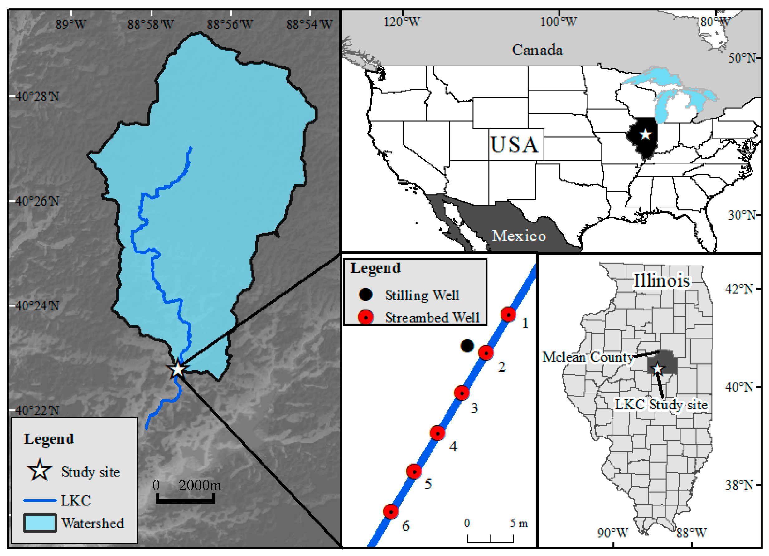
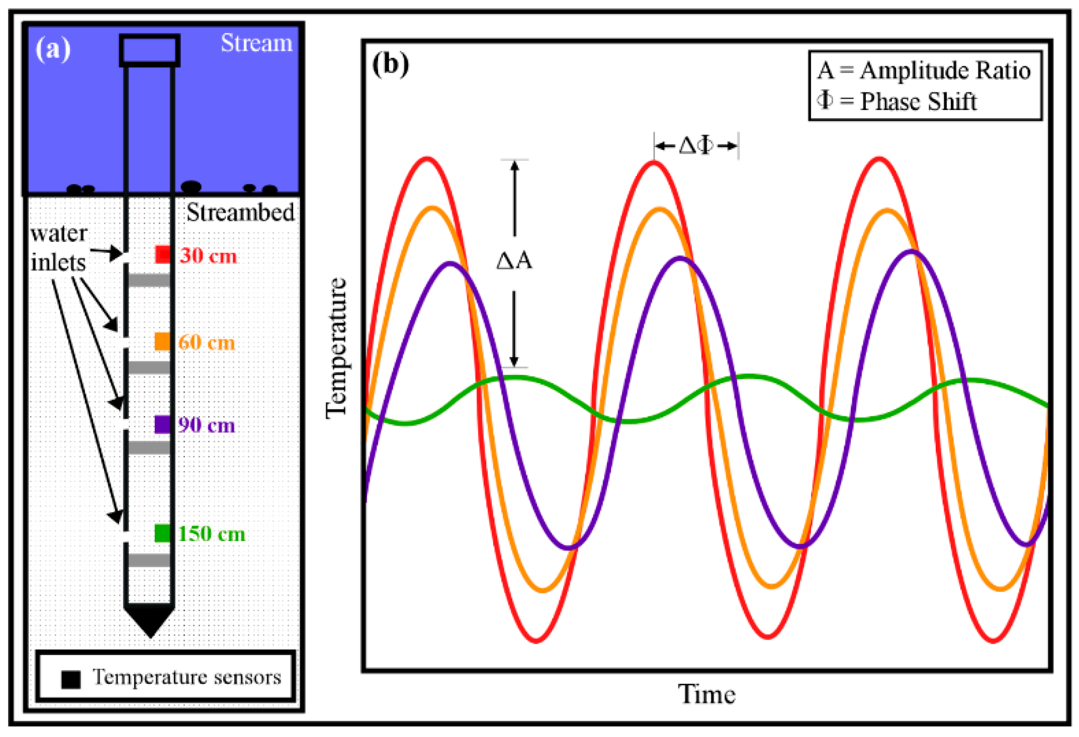
Six multi-level samplers were installed along the thalweg of a 25 m stretch of LKC (Figure 1; [32,35]). The stretch was chosen because of its low sinuosity, reducing the effects of induced flow through point bars [32,37,43]. The multi-level samplers were longitudinally positioned at 5 m intervals with the first sampler located upstream and the sixth sampler downstream. A stilling well, recording stage at a 15 min intervals, was located directly adjacent to sampler 2. The multi-level samplers were made of a 3.51 cm PVC pipe with four sealed chambers in each tube to prevent vertical mixing (Figure 2). Holes were drilled into each chamber to allow for thermal mixing and equilibrium of the corresponding streambed depths [32]. The multi-level samplers included a temperate sensor at four depths, 30, 60, 90, and 150 cm, logging at 15 min intervals. Sampler 1 and 6 had temperature loggers at the stream-streambed interface that recorded stream water temperature [32]. The temperature dataset includes a year of data from February 2009 to March 2010 [32].
2.3. Flux Calculations
Flux was calculated at the midpoint between each temperature sensor at depth, rendering four flux values per sampler. With the assumption that all energy was conserved, the rate of thermal energy changing in a system is the sum of individual rates of three separate mechanisms: conduction, convection (commonly referred to as ‘advection’), and internal heat generation [31]. Internal heat generation was not considered at LKC because no internal heat sources affect the hyporheic zone in this area. Conduction and convection were the mechanisms influencing heat flow in LKC; therefore, the heat transport governing equation can be manipulated to render hyporheic flux [1,15]. Vertical fluxes are calculated using a one-dimensional conduction-advection-dispersion equation:
where temperature, T, varies with time, t, and depth, z; Ke is the thermal diffusivity, n is the porosity, νf is the fluid velocity, and γ is the ratio of the volumetric heat capacity of the streambed (Cs) to the volumetric fluid heat capacity (Cw) [7,15]. The second term in the equation is the conduction-dispersion term. Conduction is dependent on Ke and the change in thermal gradient [31]. Ke is dependent on thermal dispersivity (β), baseline thermal conductivity in the absence of fluid flow (λo), νf, and the Cs [7,19,20] (Table 1).
The third term in the equation 1 represents convection, with the product of n and νf representing the fluid flux (q), which Hatch et al. [7] and Keery et al. [5] solved for flux using the attenuation of the amplitude (amplitude ratio) of sinusoidal temperature signals propagating vertically into the streambed.
The conduction-advection-dispersion equation has been modified to factor in amplitude and the periodic frequency of temperature fluctuations within the streambed [1,16]. This equation is divided into two components: amplitude dampening and a phase shift component [7]. A MATLAB toolbox, VFLUX, utilizes the forward model produced by Hatch et al. [7] to calculate a thermal front velocity [19,20]. VFLUX evaluates flux between sensor spacings and not the absolute depths of the temperature sensors. VFLUX limits the sensitivity of the forward model produced by Hatch et al. [7] to streambed scour or sediment buildup.
VFLUX makes various assumptions about the flux calculations: fluid flow is one-dimensional in the vertical direction, there is a sinusoidal temperature signal, there is no mean thermal gradient present in the streambed with depth, and the streambed is homogenous [20]. The model manages the data, resamples the data, extracts the diurnal signal using a dynamic harmonic regression, and calculates a vertical flux [19,20]. VFLUX resamples the temperature time series to 12 samples per day to limit issues of oversampling. After resampling the data, a Dynamic Harmonic Regression (DHR) isolates the fundamental diurnal temperature signal [17]. The DHR filter utilizes the CAPTAIN toolbox [17,44]. Finally, VFLUX calculates flux with the following inputs: temperature profiles at depth, sensor depths, period of the fundamental temperature signal, total porosity, thermal dispersivity of the streambed, thermal conductivity of the streambed, volumetric heat capacity of the sediment, and volumetric heat capacity of the water [19,20]. The amplitude is a calculated variable that the model extracts from the temperature signal input [19,20]. All input parameters for flux calculations are in Table 1.
2.4. Statistics: Stage and Vertical 1-D Flux
The Spearman’s rank correlation coefficient was used to describe the strength of the bivariate relationship between calculated flux and stage. The Spearman’s rank correlation was used due the non-normal distribution of the data. The Spearman’s rank coefficient of flux and stage was calculated in the R Statistical Environment [45]. The null hypothesis, no statistically significant linear correlation between stage and flux, was tested with a critical significance level of 0.05. A two-tailed test was chosen to see if there was a negative or positive correlation between stage and 1-D Vertical fluxes.
With the assumption that a change in stage would not induce an instantaneous change in flux, the correlation between stage and flux was measured with respect to forward temporal lags through cross-correlation in the R Statistical Environment. The calculated flux variable was shifted forward to a maximum of 80 h with a temporal resolution of two hours. The relationship between stage and 1-D vertical flux was evaluated at each 2 h lag with a two-tailed at critical significance level of 0.05.
3. Results
3.1. Trends in Raw Temperature Data and Vertical 1-D Flux
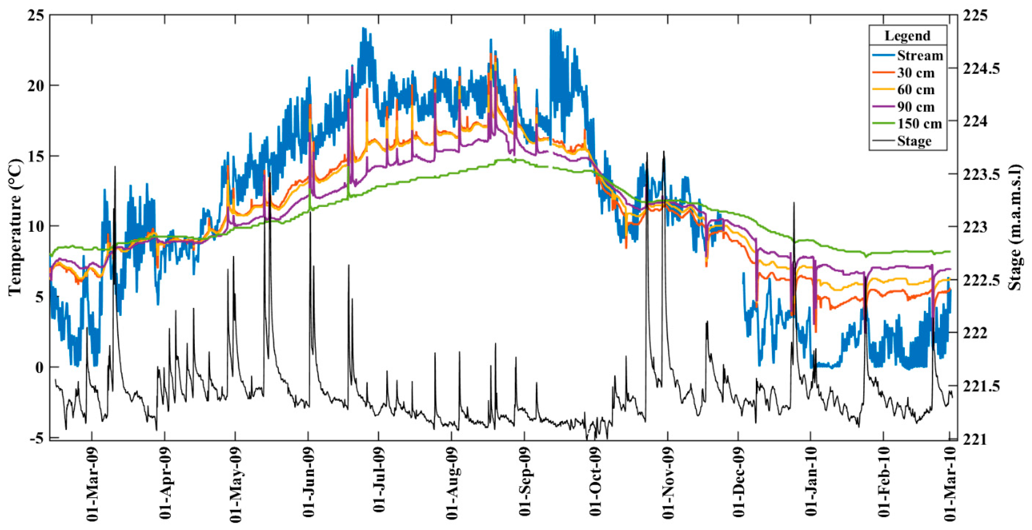
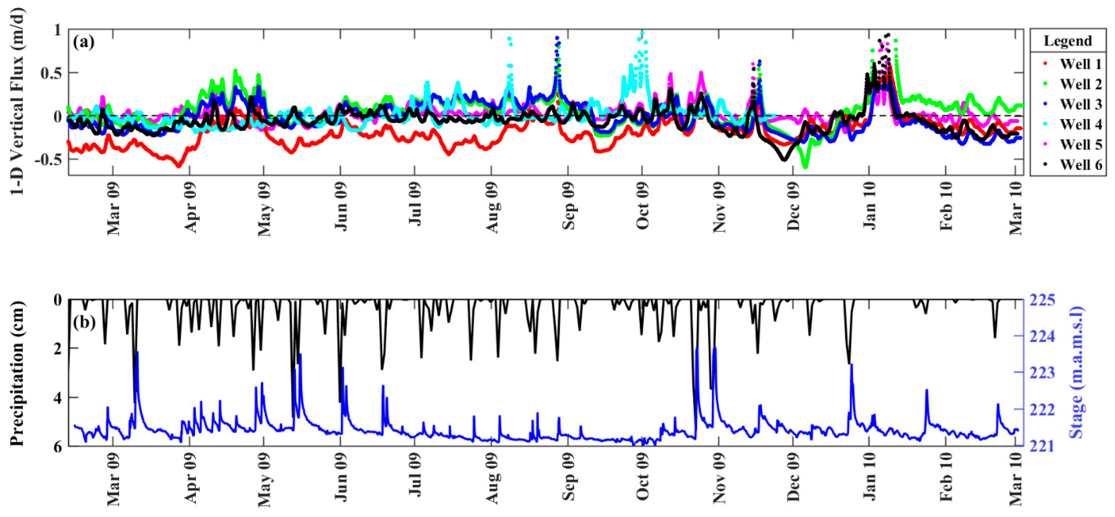
Throughout the study period, the average stage was 221.4 m above mean sea level (m.a.m.s.l.) and ranged from a 221.0 to 223.7 m.a.m.s.l. (Figure 3). Stage was lowest in the summer and highest from fall to late spring. Recharge events occurred throughout the duration of data collection, as seen in the stage response. Despite receiving less precipitation in the winter, the dormant vegetation and lack of infiltration generated recession curves that were larger in both magnitude and duration than the other seasons. Summer storms had lower peak flows and returned to baseflow equilibrium faster than the other seasons.
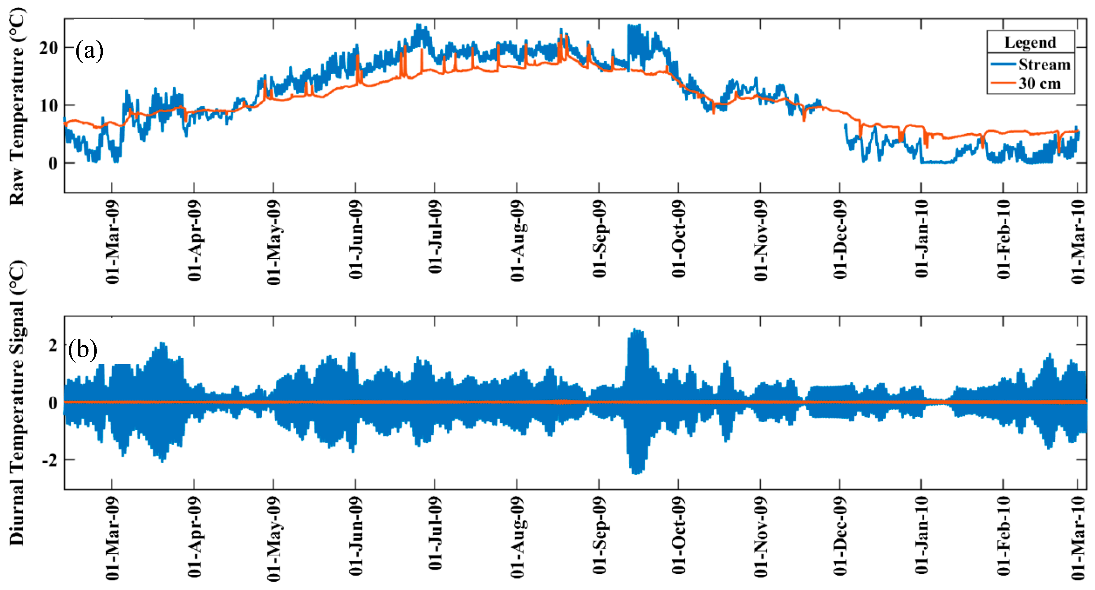
The temperatures recorded at the given depths among the samplers followed similar trends and had minimal differences. To limit redundancy, only the temperatures observed in sampler 1 are presented as they were representative observed temperatures within the other five samplers. The 13-month stream temperature time series of sampler 1 followed a sinusoidal curve with a maximum temperature of 24.08 °C in June and a minimum of −0.23 °C in February (Figure 3). Diurnal sinusoidal signatures overlaid the annual sinusoidal signal with an average daily temperature change of 2.11 °C. Three apparent temporal trends were observed in the raw 13-month temperature time series at depth for all six multi-level samplers: (1) temperature decreases with depth from May to October; (2) temperature increases with depth from October to May; and (3) the temperature trends were consistent among the samplers. In the summer and winter, the deeper hyporheic zone water temperatures were moderated by the upwelling surface water compared to the influence of the surface water in the shallow depths. Average daily stream temperature fluctuations of 2.39 °C and 1.74 °C were observed between May to October and December to March, respectively. Despite average daily temperature fluctuations of 2.48 °C, spring (March–May), and 1.62 °C, fall (October–December), that were similar in magnitude to the summer and winter, the vertical temperature profile (stream, 30, 60, 90, 150 cm) was relatively homogenous during the spring and fall periods. The similarity of the surface water and groundwater temperatures in the spring and fall are a result of the warming and cooling occurring during the periods. The homogenization masked the influence of either source, groundwater or surface water, in the streambed temperature. The uniformity of temperature within the streambed inhibited propagation of a strong diurnal signal.
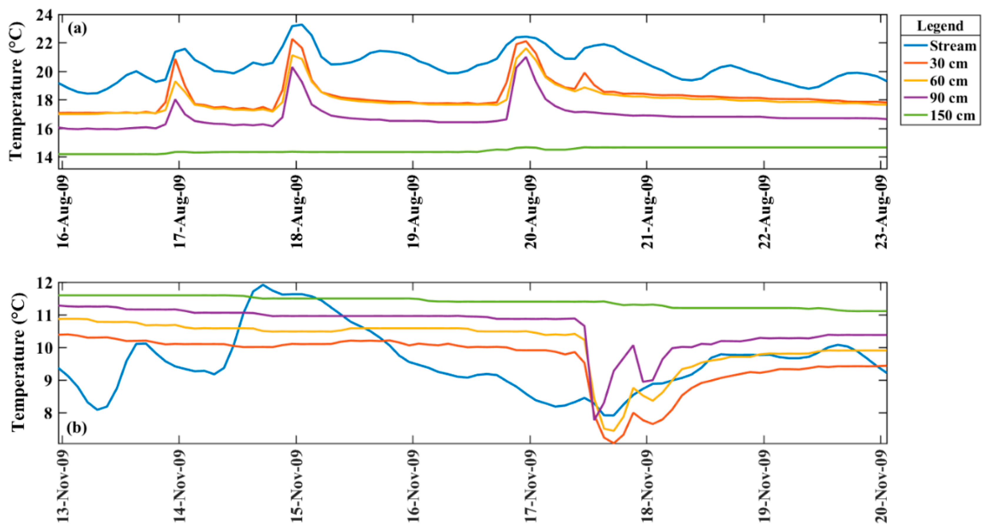
The temperature time series had two temperature gradient inflection points occurring at the onset of summer and winter (May and October). Spring and fall exhibited homogenous temperatures with depth, resulting in temperature gradients with small fluctuations. In 2009, the spring temperature gradient (stream to 150 cm) ranged from −0.038 to 0.056 °C/cm with an average of 0.0025 °C/cm. The fall displayed a similar trend of shifting temperature gradients ranging from −0.020 to 0.025 °C/cm with an average of 0.004 °C/cm. The summer season exhibited a large negative temperature gradient compared to the spring, fall, and winter ranging from −0.078 to −0.002 °C/cm with an average of −0.035 °C/cm. The 2009 winter season (February 2009) showed a positive temperature gradient ranging from 0.003 to 0.057 °C/cm with an average of 0.035 °C/cm. The 2010 winter season (December to March 2010) presented a positive temperature gradient that ranged from 0.012 to 0.067 °C/cm with an average of 0.045 °C/cm. Summer and winter had average temperature gradients an order of magnitude larger than spring and fall.
Across all seasons, the stream temperature has a diel signal that did not propagate to a streambed depth of 150 cm (Figure 3 and Table 2). Amplitudes decrease with increasing depth with an extinction between 90 to 150 cm depth. The 2009 winter, summer, fall, and winter 2010 have diel signals down to 90 cm depth. In the spring, the diel signature is extinct at 90 cm (Table 2). The entire time series has an average amplitude of 0.02 down to 90 cm depth. The streambed temperature signals at depths of 30, 60, and 90 cm are influenced by diel variations in stream temperature that propagate through the streambed as dampened signals (Figure 4).
The time series was resampled to a temporal resolution of 2 h, which was used in VFLUX to calculate the vertical flux. The raw temperature time series was filtered using the DHR model, which isolates the diurnal signal and calculates the amplitude of the thermal signal every 2 h, to extract the fundamental temperature signal used to calculate fluxes at each sensor midpoint (Figure 5) [17,44]. The calculated vertical flux revealed an increasing variation in magnitude with increasing depth. Flux was stable at a depth of 15 cm when compared to the 45, 75, and 120 cm midpoint. The shallow sub-surface (15 cm) had a dominantly negative flux (Figure 6). Negative flux indicates downward movement into the streambed, and positive flux specifies upward movement towards the stream. The flux direction is upward (positive flux) at the 45, 75, and 120 cm midpoints. At 45 cm and below, the magnitude of flux is highly variable with high-frequency spikes and missing calculations. The missing flux values occur when the VFLUX program rejects calculations due to the amplitude ratio (Ar) being greater than 1, or the program failing to converge on a root value of the thermal front velocity [7,19]. Values of Ar that are too low (Ar ≤ 0) or too high (Ar ≥ 1) result in significant errors in calculated flux [7,19]. The miscalculations can be a result of a missing solar component (diel surface signal) at depth or the sensor spacing being too large [7,19]. The deeper sensor pairs (45 and 75 cm, 90 and 150 cm) did not receive adequate surface diurnal signals resulting in too small of amplitudes. The transmission of the diurnal signal is weak at depths below 15 cm, and the streambed temperatures do not create an amplitude difference large enough (amplitude ratio approaching 1) to provide appropriate and reliable flux calculations throughout the time series. While the stream temperature signal weakens with increasing depth, it is still present up to 90cm of depth (Table 2). Flux at 15 cm is filtered to where Ar ≥ 0.9, filtering out less than 1% of the fluxes (Figure 6). Across all six streambed multi-level samplers, the percentage of Ar ≥ 0.9 at depths of 45, 75, and 90 cm is 4.54%, 17.82%, and 35.85%.
3.2. Correlation of Stage and 1-D Flux
The fluxes at the 15 cm midpoint for all six multi-level samplers ranged between −0.59 to 0.95 m/d with an average of −0.04 m/d (Figure 6a). The average flux for the 15 cm midpoint during winter 2009, spring 2009, summer 2009, fall 2009, and winter 2010 seasons are as follows: −0.09, −0.06, −0.02, −0.04, and −0.05 m/d. Throughout the 13-month time series, the 15 cm depth water is moving downward on average, but there is a temporal variation in flux as seen in Figure 6. The stream hovers around a flux of zero transitioning between gaining and losing stream conditions. In the summer, the average flux at a midpoint depth of 15 cm is low compared to the other seasons. Qualitatively, there is near-surface upwelling when stream stage is low (Summer 2009) and downwelling when stage is high (Spring 2009, Fall 2010, and Winter 2010) (Figure 6b). Quantitatively, there is a significant, but weak correlation between flux and stage at the 15 cm depth (Table 3).
The strength of the bivariate relationship between stage and flux in the near-surface streambed (15 cm) was analyzed using a two-tailed Spearman’s rank correlation test. The Spearman correlations for all six multi-level samplers at 15 cm are very weak (Table 3). Four of the multi-level samplers have a positive relationship and two exhibit a negative correlation. A negative correlation represents stage rising and flux magnitude increasing in the negative direction (losing stream condition) and vice versa. A positive correlation implies that as stage rises, flux increases in the positive or upward direction (gaining stream condition). The highest Spearman coefficient magnitude is 0.369 for sampler 4. Multi-level samplers 1, 2, 3, 5, and 6 each have correlations less than or equal to 0.15 (Table 3).
A cross-correlation analysis of stage and incremental lags in flux was interpreted using Spearman’s rank correlation (Table 3). Correlations of stage and lagged flux were calculated by keeping stage stagnant in time, while flux was temporally shifted forward with a resolution of 2 h. The max correlation between stage and flux within an 80 h window is included in the second row of Table 3. The Spearman rank correlations have p-values that are statistically significant, but very weak correlations for all six multi-level samplers. There is no apparent trend in the lag time for the maximum correlation between stage and flux at the 15 cm midpoint. Half of the 80 h window maximum correlations are negative, and the other half are positive. The highest magnitude Spearman coefficient magnitude is 0.442 at sampler 4. The other five multi-level samplers have a Spearman coefficient less than 0.20.
4. Discussion
4.1. Low-Gradient Stream Conceptual Model—Temperature and Flux dynamics
Little Kickapoo Creek is representative of Midwestern US alluvial streams characterized by its low-gradient, low-energy environment, and a streambed comprised of poorly-consolidated, mobile, glacial sediment [36]. On a watershed scale, LKC is defined as a gaining stream with an average baseflow component of 0.1 m3/s that can rise to 4 m3/s with increases in runoff and tile drainage input [34,37]. The 1-D flux data illustrate the strong upwelling component but also reveal occurrence of downwelling water.
In LKC, 1-D fluxes fluctuate between positive and negative values indicating groundwater-stream water mixing to a depth of 15 cm (Figure 6). Temperature gradients in the fall and spring are a magnitude smaller than the summer and winter representing periods of thermal equilibrium. For example, in the fall, the surface waters are cooling and begin to converge towards the temperature of the upwelling groundwater. (Figure 3). In the near-surface streambed (15 cm), hyporheic fluxes transition from downwelling conditions in the fall, winter, and spring to limited upward flux rates or flux rates approaching zero in the summer (Figure 6). At streambed depths between 15 cm to 120 cm, the mean flow direction is positive or upwards. Propagation of the stream diel temperature signal is limited to the near-subsurface due to the upwelling groundwater having a stronger influence on streambed temperatures from 60 to 150 cm mitigating the presence of a diel signal. Penetration of a robust diel stream temperature will occur in losing stream conditions by advection and will be less prominent during neutral conductive conditions (flux = 0) or gaining stream conditions [7].
Overall, hyporheic mixing occurs near the streambed with seasonal variation as groundwater upwells. Supporting this concept, hyporheic zone upwelling aligns with the gaining stream results seen in past studies [32,37,38,48]. Employing the same dataset, Bastola and Peterson [32] developed a VS2DH numerical temperature model that illustrated advective heat transport in the upward direction. The VS2DH best-fit model rendered average flux rates of 10−1 to 10−2 m/d across the 4 m vertical streambed domain, with lower rates during the wet winter and higher rates in the dry summer due to evapotranspiration [32]. The magnitude of flux rates produced in the VS2DH model aligns with the rates calculated in this study, and the direction of advective heat transfer is consistent with the groundwater upwelling from 15 to 120 cm seen in the streambed. Downward flux rates in the top 15 cm of the streambed are not observed in the VS2DH model, but the VS2DH model has a coarser spatial resolution of 1 m compared to the 30 and 60 cm resolution used in VFLUX. The coarse resolution smooths out discrete changes in flux seen at 15 cm due to spatial calculation frequency being too small the VS2DH model. Bastola and Peterson [32] reported the influence of the stream on the temperature to a depth of 30 cm suggesting the near-surface hyporheic zone is more dynamic than the deeper substrate. This study exhibits a stronger capability to see small spatial changes in fluxes in the LKC hyporheic zone. Thermal envelopes illustrated a stream influence in the top 50 cm depth of the streambed [32] similar to the groundwater transition zone seen in this study. Overall, LKC temperature models display upward groundwater advection dominating the LKC streambed, and LKC solute models point to hyporheic mixing conditions in the near-subsurface with deeper groundwater upwelling.
Temperature is a non-reactive conservative tracer, and the transport mechanisms will vary from that of conservative solutes. Thermal energy transfer in the streambed is governed by conduction and advection and will change naturally in response to the upper-boundary condition, while conservative solutes are explained by diffusion and advection. Thermal energy does not change into another form of energy, but heat is lost in the streambed due to the high heat capacity of the streambed matrix. The use of heat as a tracer is constrained to a shallower depth of the hyporheic zone when compared to solute studies due to its non-conservative nature. The spatial scale of heat tracing studies is dependent on the rate of hyporheic movement through the solid streambed matrix. In streams with lower flux rates such as LKC, the spatial scale will be smaller than studies with higher flux rates. LKC solute models reported similar depths of surface water-groundwater transition zones and percent stream water composition at depth compared to the thermal models. A chloride mixing model for the observed stretch of LKC found stream water composition of 50% at 90 to 130 cm depth in the streambed with a decline in stream water percent in the summer season [33]. Peterson and Hayden [34], concluded that the transition zone between the hyporheic zone and groundwater is between 90 and 150 cm depth in the fall and winter when groundwater upwelling occurred and decreases between 60 to 90 cm in the summer when conditions favored downwelling. Both chemical mixing models report decreased surface water composition at streambed depth during the summer months explaining the limited amount of hyporheic mixing occurring in the summer (Figure 6). During the summer, groundwater upwelling dominates the hyporheic zone and hyporheic mixing is limited. Bastola and Peterson [32] best-fit models approximated similar surface water extinction depths to Peterson and Hayden [34] and Buyck [33] at approximately 1 m in the summer and winter and 3 m in the spring. Extinction depths, defined by the terminus of a diurnal signal in the shallow substrate, do not accurately represent hyporheic flow depths. Thermal models are spatially limited due to the non-conservative nature that constrains the depth that hyporheic water is identified within the streambed. Fall and spring temperature profiles are homogenous with depth. In the fall and spring, the stream thermal signal will propagate into the streambed at a greater depth compared to the summer and winter with a larger temperature gradient across the streambed profile. Significant differences in streambed and stream temperatures will mute stream temperature signals at a shallower depth due to competing groundwater temperature. The advantage of the VFLUX model results is the fine temporal resolution and discrete flux calculations with depth that give rise to transient mixing conditions in the near-surface streambed with deeper groundwater upwelling.
4.2. Stage as a Control of 1-D Vertical Flux
Along the LKC stretch, stage exhibits weak statistically significant correlations to fluxes at the 15 cm midpoint within the near-surface hyporheic zone. The bivariate relationship is both positive and negative. Stage and discharge are expected to elevate the pressure gradient along the streambed increasing the magnitude of flux in the downward direction by vertical compression (negative correlation). Stage is not the only variable contributing to flux, and other variables such as stream velocity need to be accounted for in the fluid potential calculation [25]. Sickbert and Peterson [25] found that total head in the shallow subsurface of LKC increased less than the corresponding stage increase. The lower head values reflect the effect of velocity increases associated with the high stage. Bernoulli’s Equation explains that an increase in fluid velocity will result in a pressure reduction. The resulting decrease in pressure from an increased velocity creates a fluid-lift force that lessens the influence of the head exerted by stage on the hydraulic head in the hyporheic zone and resulting fluxes. As stage increases, the stream velocity increases, reducing the vertical head gradient due to the reduced pressure. [25]. A rise in stage not only raises the total hydraulic head in the streambed, but the resulting velocity increase by a rise in stage will alleviate and reduce the total vertical pressure gradient due to the fluid lift force. If the pressure reduction due to an increase in velocity is large enough, it could hypothetically reverse the pressure gradient creating a negative suction head in the stream. This may explain the weak positive correlations seen between stage and flux at the 15 cm midpoint depth in Table 3. Again, a positive correlation between stage and flux implies that as stream stage rises, hyporheic fluxes increase in the upward direction (gaining stream condition). Stream velocity should be accounted for, and it is invalid to assume that stage alone will control the magnitude and direction of hyporheic flux. Stage does not have a strong correlation to vertical 1-D flux in LKC with Bernoulli’s lift force being a likely candidate contributing to the control of hyporheic flux.
The weak correlation between stage and flux in the near-surface streambed (15 cm) is a possible reflection of the stage magnitude variance being too small to influence or reverse the regional pressure gradient serving as a minor control on hyporheic flow. Peterson and Hayden [34] found that stage closely mirrors the groundwater elevation, but the elevation of groundwater near the stream is higher than the stream. The lateral gradient towards the stream is the highest in the fall and summer inducing strong groundwater upwelling in the summer months. The hyporheic zone has a limited capacity to take in water, which is controlled by potential and kinetic energy gradients. There is a sharp contrast in the hydraulic conductivity between the stream and the streambed limiting flux into the streambed without a pressure gradient. Studies looking at controls on hyporheic exchange have focused on microfeatures in the streambed that have longitudinal pressure gradients that induce flow into the streambed bedforms. This phenomenon is seen in streambeds with wave-like bedforms, bars, riffles, and pools. As stage rises, bedforms along the stream bed will allow a flux initially due to a longitudinal differential pressure across the bedform, but the fluxes decrease as a longitudinal pressure gradient is eliminated by a rise in stage. Storey et al. [28] found that high stage did not correlate to higher hyporheic exchange in bedforms and saw increases in exchange when stage was low, and the water surface followed the streambed topography.
Visual evaluation of the data (Figure 6) suggests a connection between stage and flux at the 15cm midpoint streambed depth, with flux rates close to zero or positive (upwelling) when stage is lowest in the summer and opposite for the fall, spring, and winter. It is likely that multiple variables are governing hyporheic exchange. The following hydrodynamic and geomorphic variables are potential predictors of hyporheic exchange rates: streambed morphology, streambed conductivity, channel slope, stream sinuosity, horizontal stream velocity, hydraulic and vertical gradient in the microscopic stream-streambed and watershed scale, and stream stage or discharge that control the hyporheic flux [21,24,26,27,49,50]. The LKC study site was selected due to the stream segment’s low sinuosity and lack of geomorphic features such as riffles, bars, steps, and pools. Morphologic features and strong curvatures in a longitudinal stream profile should have a minor control on hyporheic exchange at the LKC location since there is a lack of these features at the study site. Although low-gradient meandering streams can have active hyporheic zones within meander lobe necks [37], Ward et al. [21] found that hydraulic gradients parallel and perpendicular to the stream bank are not sufficient predictors of hyporheic exchange flux alone. The extent of the hyporheic zone does vary with flow rate, but there are no absolute trends [21]. Several studies show that a wide range in stream discharge, a proxy for stage, has minor variation or influence in hyporheic exchange flow paths, flux, or residence time [22,24].
5. Conclusions
LKC is a low-gradient stream with an actively mixing hyporheic zone in the top 15 cm during the winter, spring, and fall with deeper upwelling groundwater. Above 15 cm the LKC hyporheic zone is actively mixing, with a negligible exchange in the summer as flux rates approached zero. Across the 14-month study period, fluxes had the highest magnitude in winter and spring. The lowest flux rates occurred in the summer when stage was low compared to other seasons.
The results of this study highlight hyporheic flux as a multivariate function that cannot be determined solely by stage. Hyporheic flux in the near-surface streambed (15 cm) is not a function of purely hydrostatic processes and the hydrodynamic and geomorphic controls should be further investigated. Stage is a weak variable contributing to fluxes, but the 15 cm fluxes converge to zero when stage is lowest in the summer. A multivariate regression analysis is advised to better understand the variables that are controlling the magnitude and direction of flux. Discovering the relationship between the regional gradient and flux is crucial to understanding the mechanisms of hyporheic exchange. There were no nearby multi-level samplers with recorded head values to obtain a regional gradient during the study period.
Author Contributions
Conceptualization, F.C.H. and E.W.P.; methodology, F.C.H. and E.W.P.; software, F.C.H.; validation, F.C.H. and E.W.P.; formal analysis, F.C.H. and E.W.P.; investigation, F.C.H. and E.W.P.; resources, F.C.H. and E.W.P.; data curation, E.W.P.; writing—original draft preparation, F.C.H. and E.W.P.; writing—review and editing, E.W.P. and F.C.H.; visualization, F.C.H. and E.W.P.; supervision, E.W.P.; project administration, E.W.P. All authors have read and agreed to the published version of the manuscript.
Funding
This research received no external funding.
Conflicts of Interest
The authors declare no conflict of interest.
References
- Stallman, R.W. Steady One-Dimensional Fluid Flow in a Semi-Infinite Porous Medium with Sinusoidal Surface Temperature. J. Geophys. Res. 1965, 70, 2821–2827. [Google Scholar] [CrossRef]
- Suzuki, S. Percolation measurements based on heat flow through soil with special reference to paddy fields. J. Geophys. Res. 1960, 65, 2883–2885. [Google Scholar] [CrossRef]
- Conant, B., Jr. Delineating and quantifying ground water discharge zones using streambed temperatures. Ground Water 2004, 42, 243–257. [Google Scholar] [CrossRef] [PubMed]
- Silliman, S.E.; Booth, D.F. Analysis of time-series measurements of sediment temperature for identification of gaining vs. losing portions of Juday Creek, Indiana. J. Hydrol. 1993, 146, 131–148. [Google Scholar] [CrossRef]
- Keery, J.; Binleya, A.; Crook, N.; Smith, J.W.N. Temporal and spatial variability of groundwater–surface water fluxes: Development and application of an analytical method using temperature time series. J. Hydrol. 2007, 336, 1–16. [Google Scholar] [CrossRef]
- Schmidt, C.; Conant, B., Jr.; Bayer-Raich, M.; Schirmer, M. Evaluation and field-scale application of a simple analytical method to quantify groundwater discharge using mapped streambed temperatures. J. Hydrol. 2007, 347, 292–307. [Google Scholar] [CrossRef]
- Hatch, C.E.; Fisher, A.T.; Revenaugh, J.S.; Constantz, J.; Ruehl, C. Quantifying surface water-groundwater interactions using time series analysis of streambed thermal records: Method development. Water Resour. Res. 2006, 42. [Google Scholar] [CrossRef] [Green Version]
- Becker, M.W.; Georgian, T.; Ambrose, H.; Siniscalchi, J.; Fredrick, K. Estimating flow and flux of ground water discharge using water temperature and velocity. J. Hydrol. 2004, 296, 221–233. [Google Scholar] [CrossRef]
- Lapham, W.W. Use of Temperature Profiles Beneath Streams to Determine Rates of Vertical Ground-Water Flow and Vertical Hydraulic Conductivity; 0886-9308; United States Geological Survey: Reston, VA, USA, 1989; p. 35. [Google Scholar]
- Briggs, M.A.; Lautz, L.K.; Buckley, S.F.; Lane, J.W. Practical limitations on the use of diurnal temperature signals to quantify groundwater upwelling. J. Hydrol. 2014, 519, 1739–1751. [Google Scholar] [CrossRef]
- Jensen, J.K.; Engesgaard, P. Nonuniform Groundwater Discharge across a Streambed: Heat as a Tracer. Vadose Zone J. 2011, 10, 98–109. [Google Scholar] [CrossRef]
- Allander, K. Trout Creek—Evaluating ground-water and surface water exchange along an alpine stream, Lake Tahoe, California. In Heat as a Tool for Studying the Movement of Ground Water Near Streams; Stonestrom, D.A., Constantz, J., Eds.; United States Geological Survey: Reston, VA, USA, 2003; Volume Circular 1260, pp. 35–45. [Google Scholar]
- Luce, C.H.; Tonina, D.; Gariglio, F.; Applebee, R. Solutions for the diurnally forced advection-diffusion equation to estimate bulk fluid velocity and diffusivity in streambeds from temperature time series. Water Resour. Res. 2013, 49, 488–506. [Google Scholar] [CrossRef] [Green Version]
- McCallum, A.M.; Andersen, M.S.; Rau, G.C.; Acworth, R.I. A 1-D analytical method for estimating surface water–groundwater interactions and effective thermal diffusivity using temperature time series. Water Resour. Res. 2012, 48. [Google Scholar] [CrossRef]
- Anderson, M.P. Heat as a ground water tracer. Ground Water 2005, 43, 951–968. [Google Scholar] [CrossRef] [PubMed]
- Goto, S.; Yamano, M.; Kinoshita, M. Thermal response of sediment with vertical fluid flow to periodic temperature variation at the surface. J. Geophys. Res. Sol. Earth 2005, 110. [Google Scholar] [CrossRef]
- Young, P.C.; Pedregal, D.J.; Tych, W. Dynamic harmonic regression. J. Forecast. 1999, 18, 369–394. [Google Scholar] [CrossRef] [Green Version]
- Swanson, T.E.; Cardenas, M.B. Ex-Stream: A MATLAB program for calculating fluid flux through sediment–water interfaces based on steady and transient temperature profiles. Comput. Geosci. 2011, 37, 1664–1669. [Google Scholar] [CrossRef]
- Gordon, R.P.; Lautz, L.K.; Briggs, M.A.; McKenzie, J.M. Automated calculation of vertical pore-water flux from field temperature time series using the VFLUX method and computer program. J. Hydrol. 2012, 420, 142–158. [Google Scholar] [CrossRef]
- Irvine, D.J.; Lautz, L.K.; Briggs, M.A.; Gordon, R.P.; McKenzie, J.M. Experimental evaluation of the applicability of phase, amplitude, and combined methods to determine water flux and thermal diffusivity from temperature time series using VFLUX 2. J. Hydrol. 2015, 531, 728–737. [Google Scholar] [CrossRef] [Green Version]
- Ward, A.S.; Fitzgerald, M.; Gooseff, M.N.; Voltz, T.J.; Binley, A.M.; Singha, K. Hydrologic and geomorphic controls on hyporheic exchange during base flow recession in a headwater mountain stream. Water Resour. Res. 2012, 48. [Google Scholar] [CrossRef] [Green Version]
- Ward, A.S.; Schmadel, N.M.; Wondzell, S.M.; Gooseff, M.N.; Singha, K. Dynamic hyporheic and riparian flow path geometry through base flow recession in two headwater mountain stream corridors. Water Resour. Res. 2017, 53, 3988–4003. [Google Scholar] [CrossRef]
- Ward, A.S.; Schmadel, N.M.; Wondzell, S.M.; Harman, C.; Gooseff, M.N.; Singha, K. Hydrogeomorphic controls on hyporheic and riparian transport in two headwater mountain streams during base flow recession. Water Resour. Res. 2016, 52, 1479–1497. [Google Scholar] [CrossRef]
- Schmadel, N.M.; Ward, A.S.; Wondzell, S.M. Hydrologic controls on hyporheic exchange in a headwater mountain stream. Water Resour. Res. 2017, 53, 6260–6278. [Google Scholar] [CrossRef]
- Sickbert, T.B.; Peterson, E.W. The effect of surface water velocity on hyporheic interchange. J. Water Resour. Prot. 2014, 6, 327–336. [Google Scholar] [CrossRef] [Green Version]
- Harvey, J.W.; Bencala, K.E. The effect of streambed topography on surface-subsurface water exchange in mountain catchments. Water Resour. Res. 1993, 29, 89–98. [Google Scholar] [CrossRef]
- Kasahara, T.; Wondzell, S.M. Geomorphic controls on hyporheic exchange flow in mountain streams. Water Resour. Res. 2003, 39. [Google Scholar] [CrossRef] [Green Version]
- Storey, R.G.; Howard, K.W.F.; Williams, D.D. Factors controlling riffle-scale hyporheic exchange flows and their seasonal changes in a gaining stream; a three-dimensional groundwater flow model. Water Resour. Res. 2003, 39. [Google Scholar] [CrossRef]
- Wondzell, S.M.; Gooseff, M.N. Geomorphic controls on hyporheic exchange across scales: Watersheds to particles. In Treatise on Geomorphology; Shroder, J., Wohl, E., Eds.; Academic Press: San Diego, CA, USA, 2013; Volume 9, pp. 203–218. [Google Scholar]
- Cardenas, M.B.; Wilson, J.L.; Zlotnik, V.A. Impact of heterogeneity, bed forms, and stream curvature on subchannel hyporheic exchange. Water Resour. Res. 2004, 40. [Google Scholar] [CrossRef] [Green Version]
- Deming, D. Introduction to Hydrogeology; McGraw-Hill College: New York, NY, USA, 2002; p. 468. [Google Scholar]
- Bastola, H.; Peterson, E.W. Heat tracing to examine seasonal groundwater flow beneath a low-gradient stream. Hydrogeol. J. 2016, 24, 181–194. [Google Scholar] [CrossRef]
- Buyck, M.S. Tracking Nitrate Loss and Modeling Flow through the Hyporheic Zone of a Low Gradient Stream through the Use of Conservative Tracers. Master’s Thesis, Illinois State University, Normal, IL, USA, 2005. [Google Scholar]
- Peterson, E.W.; Hayden, K.M. Transport and Fate of Nitrate in the Streambed of a Low-Gradient Stream. Hydrology 2018, 5, 55. [Google Scholar] [CrossRef] [Green Version]
- Oware, E. The Impact of Storm on Thermal Transport in the Hyporheic Zone of a Low-Gradient Third-Order Sand and Gravel Bedded Stream. Master’s Thesis, Illinois State University, Normal, IL, USA, 2010. [Google Scholar]
- Peterson, E.W.; Sickbert, T.B.; Moore, S.L. High frequency stream bed mobility of a low-gradient agricultural stream with implications on the hyporheic zone. Hydrol. Process. 2008, 22, 4239–4248. [Google Scholar] [CrossRef]
- Peterson, E.W.; Sickbert, T.B. Stream water bypass through a meander neck, laterally extending the hyporheic zone. Hydrogeol. J. 2006, 14, 1443–1451. [Google Scholar] [CrossRef]
- Peterson, E.W.; Benning, C. Factors influencing nitrate within a low-gradient agricultural stream. Environ. Earth Sci. 2013, 68, 1233–1245. [Google Scholar] [CrossRef]
- Riggs, M.H.; Abert, C.C. Cumulative sand and gravel thickness in McLean County, Illinois. In Open File Series 1997-01f; Survey, I.S.G., Ed.; Illinois State Geological Survey: Champaign, IL, USA, 1998. [Google Scholar]
- Hansel, A.K.; Johnson, W.H. Wedron and Mason Groups: Lithostratigraphic Reclassification of Deposits of the Wisconsin Episode, Lake Michigan Lobe Area; Bulletin 104; Illinois State Geological Survey: Champaign, IL, USA, 1996; p. 116. [Google Scholar]
- Basu, A. Quantifying N Cycling Between Groundwater and Surface Water Using Numerical Modeling and Mass Flux Calculations. Master’s Thesis, Illinois State University, Normal, IL, USA, 2007. [Google Scholar]
- Ackerman, J.R.; Peterson, E.W.; Van der Hoven, S.; Perry, W. Quantifying nutrient removal from groundwater seepage out of constructed wetlands receiving treated wastewater effluent. Environ. Earth Sci. 2015, 74, 1633–1645. [Google Scholar] [CrossRef]
- Van der Hoven, S.J.; Fromm, N.J.; Peterson, E.W. Quantifying nitrogen cycling beneath a meander of a low gradient, N-impacted, agricultural stream using tracers and numerical modelling. Hydrol. Process. 2008, 22, 1206–1215. [Google Scholar] [CrossRef]
- Young, P.; Taylor, C.; Tych, W.; Pegregal, D.; McKenna, P. The Captain Toolbox. In Centre for Research on Environmental Systems and Statistics; Lancaster University: Bailrigg, UK, 2010. [Google Scholar]
- R Core Team. R: A Language and Environment for Statistical Computing; R Foundation for Statistical Computing: Vienna, Austria, 2013. [Google Scholar]
- Irvine, D.J.; Briggs, M.; Cartwright, I.; Lautz, L. Improved vertical streambed flux estimation using multiple diurnal temperature methods in series. Groundwater 2016, 55, 73–80. [Google Scholar] [CrossRef] [Green Version]
- Irvine, D.J.; Briggs, M.A.; Lautz, L.K.; Gordon, R.P.; McKenzie, J.M.; Cartwright, I. Using Diurnal Temperature Signals to Infer Vertical Groundwater-Surface Water Exchange. Groundwater 2017, 55, 1–17. [Google Scholar] [CrossRef]
- Beach, V.; Peterson, E.W. Variation of hyporheic temperature profiles in a low gradient third-order agricultural stream–A statistical approach. Open J. Mod. Hydrol. 2013, 3, 55–66. [Google Scholar] [CrossRef] [Green Version]
- Hester, E.T.; Doyle, M.W. In-stream geomorphic structures as drivers of hyporheic exchange. Water Resour. Res. 2008, 44. [Google Scholar] [CrossRef]
- Hill, A.R.; Labadia, C.F.; Sanmugadas, K. Hyporheic zone hydrology and nitrogen dynamics in relation to the streambed topography of a N-rich stream. Biogeochemistry 1998, 42, 285–310. [Google Scholar] [CrossRef]
Figure 1.
Little Kickapoo Creek (LKC) watershed and the site configuration in plan view. There are six streambed multi-level samplers installed along the thalweg of the stream. The stilling well, installed along the stream bank in-line with the second multi-level sampler, monitored stage at a 15 min intervals.

Figure 2.
(a). A nested streambed sampler with four temperature sensors at 30, 60, 90, 150 cm depths. Each temperature sensor was isolated with foam sealant. (b) Phase shift and amplitude attenuation of sinusoidal thermal signals with increasing depth. The amplitude of thermal signals decreases, ∆A, and the signal is delayed, shift in phase (∆ϕ), with increasing depth in the streambed (graphic modified from [7].

Figure 3.
Stream stage and water temperature in the stream and at depths of 30, 60, 90, and 150 cm within sampler 1. Temperatures observed in sampler 1 were representative of all six samplers.
Figure 3.
Stream stage and water temperature in the stream and at depths of 30, 60, 90, and 150 cm within sampler 1. Temperatures observed in sampler 1 were representative of all six samplers.

Figure 4.
Week-long temperature time series with storm events at 30, 60, 90, 150 cm depth. There are storm events on 8/17, 8/18, 8/20, and 11/17–11/19. The summer temperature gradient is negative (a), and the winter is positive (b). The stream temperature signal change during the storm event propagates down to a streambed depth of 90 cm in the winter and summer.

Figure 5.
(a) Complete 13-month raw temperature time series. (b) The diurnal (24 h) component isolated from the raw temperature time signal by the DHR model [46,47]. The amplitude variation is minimal at a depth of 30 cm. The amplitude decreases with increasing depth.

Figure 6.
(a). Calculated Flux at 15 cm depth for all six multi-level samplers. (b). Precipitation and stage data. Stage is lowest in the summer (May–July) when flux rates are higher relative to fall, winter, and spring.
Figure 6.
(a). Calculated Flux at 15 cm depth for all six multi-level samplers. (b). Precipitation and stage data. Stage is lowest in the summer (May–July) when flux rates are higher relative to fall, winter, and spring.


Table 1.
Parameter values used in flux calculations. The parameters representative of the Henry Formation.
Table 1.
Parameter values used in flux calculations. The parameters representative of the Henry Formation.
| Parameter | Units | Value | Source |
|---|---|---|---|
| Porosity (n) | 0.375 | [32] | |
| Dispersivity (β) | m | 0.005 | [32] |
| Thermal Conductivity (λo) | cal/sec-cm-C | 0.0033 | [32] |
| Volumetric Heat Capacity of Sediment (Cs) | cal/cm3-C | 0.239 | [32] |
| Volumetric Heat Capacity of Water (Cw) | cal/cm3-C | 1 | [9] |
Table 2.
Seasonal amplitude averages at each temperature sensor depth.
| Complete Time Series | Winter 2009 | Spring 2009 | Summer 2009 | Fall 2009 | Winter 2010 | |||
|---|---|---|---|---|---|---|---|---|
| Depth | Minimum | Mean | Maximum | Mean | Mean | Mean | Mean | Mean |
| (cm) | (°C) | (°C) | (°C) | (°C) | (°C) | (°C) | (°C) | (°C) |
| Stream (0) | 0.02 | 0.85 | 2.59 | 0.86 | 0.91 | 0.99 | 0.60 | 0.62 |
| 30 | 0.00 | 0.03 | 0.07 | 0.01 | 0.02 | 0.03 | 0.03 | 0.04 |
| 60 | 0.00 | 0.02 | 0.05 | 0.01 | 0.01 | 0.02 | 0.03 | 0.03 |
| 90 | 0.00 | 0.02 | 0.13 | 0.01 | 0.00 | 0.02 | 0.01 | 0.06 |
| 150 | 0.00 | 0.00 | 0.00 | 0.00 | 0.00 | 0.00 | 0.00 | 0.00 |
Table 3.
Spearman rank correlation coefficients (ρ) for all six multi-level samplers at 15 cm midpoint depth. All ρ values were statistically significant for a 95% confidence level. The correlation coefficient in the first row is between stage and flux with no forward time step. The second row indicates the maximum ρ values between stage and flux with incremental 2 h time steps in flux up to 80 h of lag time. There are positive and negative statistically significant weak correlations between stage and flux.
| Well 1 | Well 2 | Well 3 | Well 4 | Well 5 | Well 6 | |||||||
|---|---|---|---|---|---|---|---|---|---|---|---|---|
| Lag (h) | ρ | Lag (h) | ρ | Lag (h) | ρ | Lag (h) | ρ | Lag (h) | ρ | Lag (h) | ρ | |
| No Lag | 0 | 0.14 | 0 | 0.05 | 0 | 0.09 | 0 | 0.37 | 0 | −0.11 | 0 | −0.03 |
| ρmax | 34 | 0.19 | 26 | 0.09 | 80 | −0.12 | 28 | 0.44 | 80 | −0.18 | 80 | 0.04 |
© 2020 by the authors. Licensee MDPI, Basel, Switzerland. This article is an open access article distributed under the terms and conditions of the Creative Commons Attribution (CC BY) license (http://creativecommons.org/licenses/by/4.0/).
Share and Cite
MDPI and ACS Style
Harris, F.C.; Peterson, E.W. 1-D Vertical Flux Dynamics in a Low-Gradient Stream: An Assessment of Stage as a Control of Vertical Hyporheic Exchange. Water 2020, 12, 708. https://doi.org/10.3390/w12030708
AMA Style
Harris FC, Peterson EW. 1-D Vertical Flux Dynamics in a Low-Gradient Stream: An Assessment of Stage as a Control of Vertical Hyporheic Exchange. Water. 2020; 12(3):708. https://doi.org/10.3390/w12030708
Chicago/Turabian StyleHarris, F. Claire, and Eric W. Peterson. 2020. "1-D Vertical Flux Dynamics in a Low-Gradient Stream: An Assessment of Stage as a Control of Vertical Hyporheic Exchange" Water 12, no. 3: 708. https://doi.org/10.3390/w12030708
Note that from the first issue of 2016, this journal uses article numbers instead of page numbers. See further details here.