Zooplankton Community Responses to Oxygen Stress
by
 , ,
, ,
Maciej Karpowicz
1,* ,
,
Jolanta Ejsmont-Karabin
2,
Joanna Kozłowska
1,
Irina Feniova
3 and
Andrew R. Dzialowski
4 1
Department of Hydrobiology, Faculty of Biology, University of Białystok, Ciołkowskiego 1J, 15-245 Białystok, Poland
2
Research Station in Mikołajki, Nencki Institute of Experimental Biology, Polish Academy of Sciences, 3 Pasteur Street, 02-093 Warsaw, Poland
3
Institute of Ecology and Evolution, Russian Academy of Sciences, Leninsky Prospect 33, 119071 Moscow, Russia
4
Department of Integrative Biology, Oklahoma State University, Stillwater, OK 74078, USA
*
Author to whom correspondence should be addressed.
Water 2020, 12(3), 706; https://doi.org/10.3390/w12030706
Submission received: 27 January 2020
/
Revised: 27 February 2020
/
Accepted: 28 February 2020
/
Published: 5 March 2020
(This article belongs to the Special Issue The Response of the Plankton Community to Environmental Stress)
Abstract
:Recent changes in climate and eutrophication have caused increases in oxygen depletion in both freshwater and marine ecosystems. However, the impact of oxygen stress on zooplankton, which is the major trophic link between primary producers and fish, remains largely unknown in lakes. Therefore, we studied 41 lakes with different trophic and oxygen conditions to assess the role of oxygen stress on zooplankton communities and carbon transfer between phytoplankton and zooplankton. Samples were collected from each lake at the peak of summer stratification from three depth layers (the epilimnion, metalimnion, and hypolimnion). Our results revealed that freshwater zooplankton were relatively tolerant to anoxic conditions and the greatest changes in community structure were found in lakes with the highest oxygen deficits. This caused a switch in dominance from large to small species and reduced the zooplankton biomass in lower, anoxic layers of water, but not in the upper layers of water where the oxygen deficits began. This upper anoxic layer could thus be a very important refuge for zooplankton to avoid predation during the day. However, the reduction of zooplankton in the lower water layers was the main factor that reduced the effectiveness of carbon transfer between the phytoplankton and zooplankton.
1. Introduction
The dissolved oxygen (DO) concentration in the water column is a crucial parameter for the successful development of many pelagic organisms [1]. Oxygen stress is a common phenomenon in freshwater ecosystems as lakes worldwide are increasingly experiencing the depletion of DO in the water layers below the epilimnion. Dissolved oxygen depletion results from a number of natural factors, but is most often considered a consequence of eutrophication from changes in land use [2]. Increased concentrations of nutrients favor the mass development of phytoplankton, which raises the DO saturation through photosynthesis during the day and reduces the DO saturation through respiration during the night. When the algae die, they sink towards the bottom and are decomposed by bacteria, which further reduces the DO in the water column [3]. Recent changes in the climate also contribute to hypolimnetic oxygen depletion due to higher surface water temperatures, which strengthen thermal stratification, thereby decreasing the exchange of oxygen between the epilimnion and hypolimnion [4,5,6]. A similar process has been observed for marine ecosystems, where eutrophication induced oxygen depletion was responsible for approximately half of the known dead zones [7].
Dissolved oxygen concentrations below 2 mg L−1 are referred to as hypoxic conditions, and the near-complete absence of DO (<0.5 mg L−1) is referred to as anoxic conditions [7,8,9]. Oxygen stress also depends on the water temperature, which controls both oxygen solubility and the metabolic demand of aquatic ectotherms [9]. Oxygen depletion disrupts biotic interactions and causes significant changes in freshwater food webs [10,11]. However, the oxygen tolerance and threshold values can vary considerably for different organisms [12]. Generally, fish seem to be more vulnerable to hypoxia than crustaceans and mollusks [13]. With regard to zooplankton communities, it is generally assumed that oxygen stress plays an important role in determining the community structure and vertical distribution [14,15,16]. Anoxic water layers may disrupt zooplankton diel vertical migrations, and, during the day, zooplankton may experience a trade-off between (i) increased metabolic stress and mortality due to low DO in the hypolimnion and (ii) mortality due to increased fish predation and increased cellular damage due to UV radiation exposure in the epilimnion [9,17].
Our previous research in humic lakes revealed that anoxic conditions 2–3 m below the surface were the main factor limiting the biomass and diversity of zooplankton [15]. Other field studies suggest that decreases in metalimnetic and hypolimnetic oxygen concentrations resulted in a shift in the size of zooplankton communities from large to smaller species [14,18,19]. However, other studies showed that metalimnetic hypoxia could be a refuge for large zooplankton species as they are more tolerant to lower oxygen concentrations than most pelagic fish [20,21,22,23,24]. Deep chlorophyll maxima, which are often followed by metalimnetic hypoxia, are also an additional refuge for zooplankton [25,26]. The results from field studies revealed that even glacial relicts, such as Eurytemora lacustris, were the most numerous in hypoxic metalimnia, suggesting that this species could tolerate the warmer water and lower oxygen concentrations due to better food resources [27]. Other experimental research indicated high physiological and demographic costs for zooplankton in an environment with a low oxygen concentration [28,29,30,31].
The impact of oxygen stress on pelagic organisms in lakes remains largely enigmatic, and there is a lack of evidence showing the direct impacts of oxygen stress on zooplankton communities [23,32]. This is especially important as zooplankton are a key component of freshwater food webs and biogeochemical cycles, serving as the major trophic link between primary producers (phytoplankton) and fish. Therefore, we conducted a multiple lake survey during the peak of summer stratification to assess the role of oxygen stress and eutrophication on zooplankton communities.
We hypothesized that (i) oxygen stress is the major force shaping the biomass, diversity, and size-structure of zooplankton communities in different trophic conditions; (ii) small-bodied species could have an advantage over large species in anoxic conditions; (iii) anoxic conditions significantly reduce the effectiveness of carbon transfer between phytoplankton and zooplankton. Finally, some zooplankton taxa may be less sensitive than others to oxygen stress [17,23,33]. For example, copepods may be largely unaffected by oxygen deficits until the DO concentrations are less than 1 mg L−1; whereas, larger cladoceran taxa (e.g., Daphnia) may be more sensitive to hypoxia [23]. Although rotifers were not found in truly anoxic waters, some species reached high densities at low oxygen concentrations [34]. Therefore, it is especially important to assess which zooplankton species or taxa are more prevalent under anoxic conditions. For this reason, we distinguished species that are very sensitive to oxygen stress from species that tolerated anoxic conditions.
2. Study Area and Methods
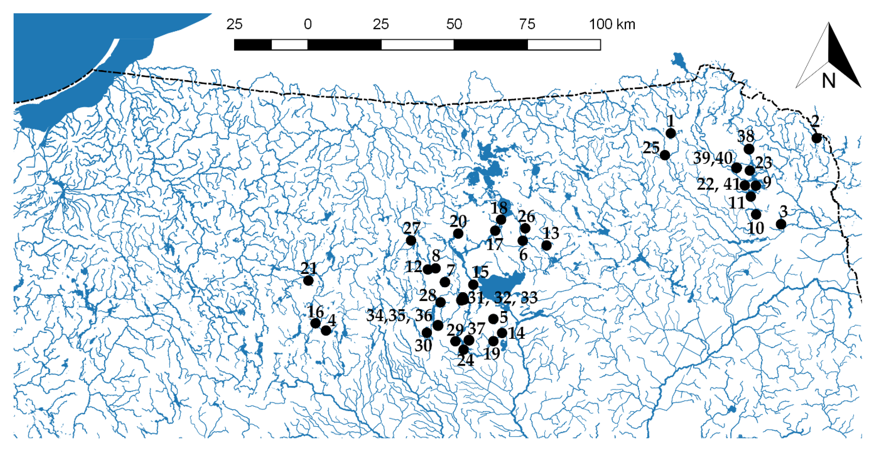
The study was conducted in 41 lakes in north-eastern Poland (Figure 1) with different morphometric parameters, trophic status, and oxygen conditions (Table 1). The area under investigation represents a typical landscape formed during the last Vistulian glacial period [35] and includes the Masurian Lakeland and Suwalki Lakeland. The maximum depth of the lakes ranged from 3 to 73 m, and the surface area ranged from 0.96 ha to 2118.3 ha. Lake Wigry was the largest and deepest, and it is distinguished by very diversified morphometry and a highly developed shoreline [16]. The smallest lakes were mid-forest dystrophic lakes (Table 1), which are usually oval, without any inflows and outflows [36].
The trophic status of the harmonic lakes was calculated using the Carlson trophic state index (TSI) as an average of three parameters: Secchi disc visibility (SDV), concentration of chlorophyll-a, and total phosphorus [37]. The lakes with a TSI below 40 were classified as oligotrophic, between 40–50 as mesotrophic, and above 50 as eutrophic. The state of dystrophy was evaluated using the hydrochemical dystrophy index (HDI) as an average for three equations, which include data for the surface water pH, electric conductivity, dissolved inorganic carbon and dissolved organic carbon concentrations [36]. The HDI values between 50 and 65 indicate semi-dystrophic conditions, while values from 65 up to 100 indicate advanced dystrophy.
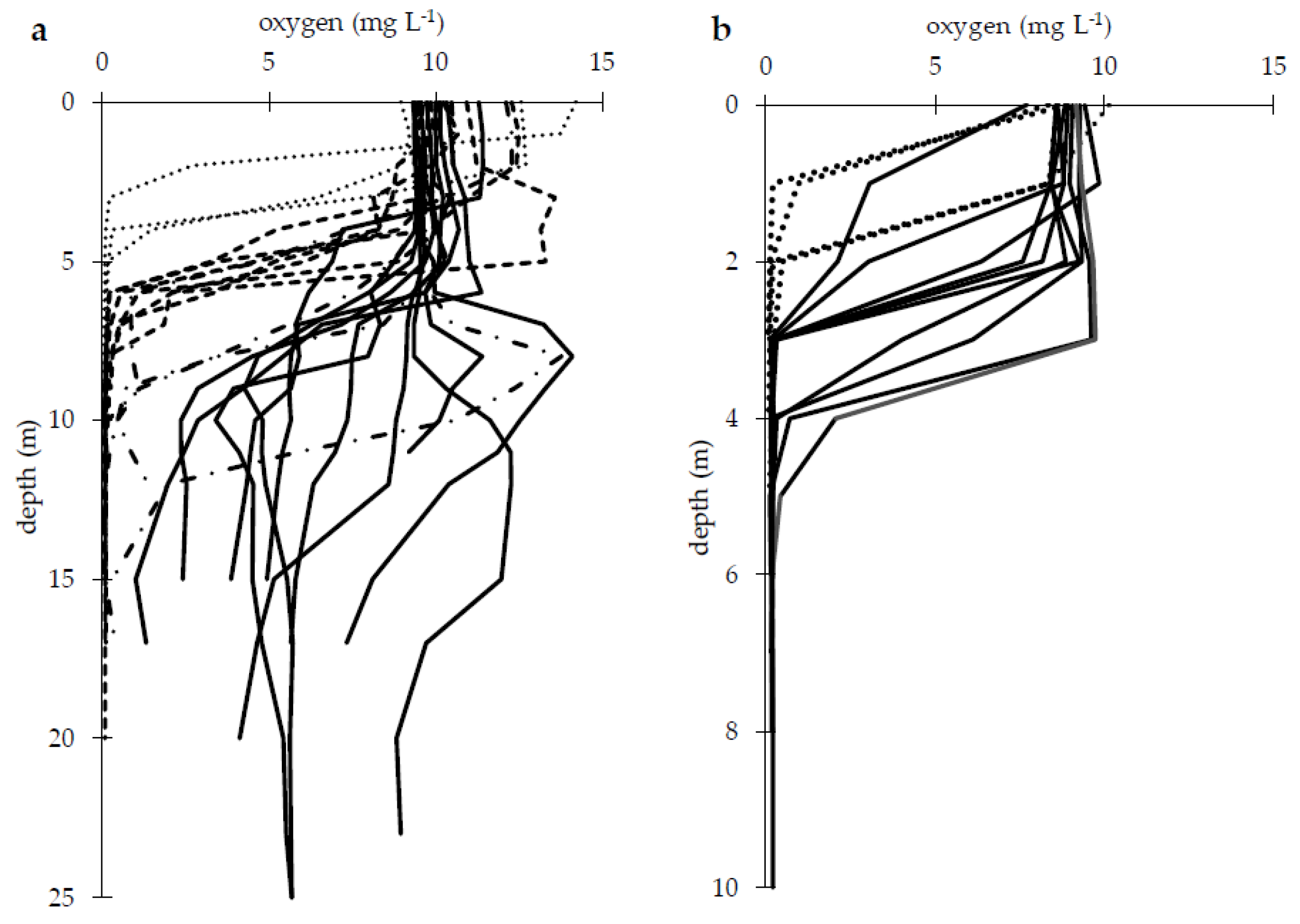
We identified 27 harmonic lakes (oligotrophic, mesotrophic, eutrophic) and 14 dystrophic lakes in our sample lakes (Table 1). The dystrophic lakes were distinguished by high HDI values from 60.4 to 79.9, with an average 70.6 (Table 1). The waters of these lakes were strongly acidic with small concentrations of mineral substances dissolved in water, but with a large amount of dissolved organic matter and humic substances [36]. Dystrophic lakes have a characteristic yellow-brown water color that results in a unique light climate and rapid warming of the epilimnion leading to strong thermal stratification [15]. The sharp thermal stratification was followed by sharp oxygen stratification, where anoxic conditions were observed even beginning at 1 m (Figure 2b). Most of the dystrophic lakes were surrounded by a coat of mosses (Sphagnum sp.) and peat, which extended in the lake to a considerable depth and were overgrown by roots of different plants and dwarf trees [15,38]. The harmonic lakes largely differed in trophic conditions and the TSI values ranged from 29.6 to 62.8 (Table 1). Five lakes were classified as oligotrophic as the Secchi disk transparency ranged from 3.8 to 7.4 m. Nine lakes were classified as mesotrophic with the SDV from 1.6 to 6.6 m. Thirteen lakes were classified as eutrophic with the SDV from 0.5 to 2.2 m (Table 1).
The lakes were also distinguished by different oxygen conditions and divided into six groups according to Figure 2. We divided the dystrophic lakes due to strong thermal and oxygen stratification and differences in the environmental parameters described above. The first group (G1) consisted of eleven lakes without anoxic conditions, the second group (G2) consisted of six lakes with anoxic conditions in the hypolimnion, the third group (G3) consisted of six lakes with anoxic conditions beginning in the metalimnion, and the fourth group (G4) consisted of four lakes with anoxia beginning in the epilimnion (Table 1, Figure 2). The dystrophic lakes were divided into lakes where anoxia started from 3–5 m (G5) and lakes with anoxia from 1–2 m (G6). Further analyses were based on this division.
There were significant differences in the depth of the epilimnion between the harmonic and dystrophic lakes (One-way ANOVA: F = 55.7; p < 0.0001). The depth of the epilimnion of dystrophic lakes ranged from 1 to 3 m, with an average of 1.8 m. In comparison, the epilimnion depth in harmonic lakes ranged from 3 to 7.5 m with an average of 5.9 m (Table 1). The average temperature of the epilimnion was 22.2 ± 1.6 °C, but there were differences in the epilimnion temperature between the harmonic and dystrophic lakes (One-way ANOVA: F = 19.6; p < 0.0001). The temperature of the epilimnion in dystrophic lakes was 23.3 ± 1.9 °C with a maximum of 27.3 °C, while in harmonic lakes it was 21.9 ± 1.4 °C with a maximum of 25.5 °C. The average metalimnion thickness was 3.3 ± 0.8 m, and there were no significant differences between lakes with different trophic and oxygen conditions (Table 1). The metalimnion temperature was 14.2 ± 3.4 °C. The hypolimnion temperature was 7.7 ± 2.0 m, and there were significant differences between the harmonic and dystrophic lakes (One-way ANOVA: F = 25.1; p < 0.0001). The hypolimnion temperature in the dystrophic lakes was 6.6 ± 1.5 °C, compared to 8.0 ± 1.9 °C in the harmonic lakes. Additionally, deep harmonic lakes (>30 m) were characterized by lower temperatures in the hypolimnion (One-way ANOVA: F = 16.4; p = 0.0001), which was 7.3 ± 1.5 °C, while in shallower harmonic lakes it was 8.9 ± 2.2 °C.
Each lake was sampled during the peak of summer stratification (end of July and beginning of August) in 2018 and 2019. The sampling stations in each lake were located close to the deepest point. The field measurements included Secchi disc visibility (SDV), dissolved oxygen, pH, and electrical conductivity using an HQ40D Multi Meter (Hach-Lange GmbH, Germany). The photosynthetic active radiation (PAR) was measured using a LI-193SA Spectral Quantum sensor (LI-COR Biosciences, Lincoln, NE, USA). The temperature and chlorophyll-a concentrations were recorded by continuous measurements using a submersible spectrofluorometer FluoroProbe (bbe-Moldaenke, Germany). This probe also determines four phytoplankton classes: green algae (Chlorophyta and Euglenophyta), cyanobacteria (phycocyanin- rich cyanobacteria), diatoms (Heterokontophyta, Haptophyta, and Dinophyta), and cryptophytes (Cryptophyta and the phycoerythrin-rich cyanobacteria) [26,39]. Field measurements of the temperature, oxygen, and chlorophyll-a were made at 1 m intervals from the surface to 30 m, while PAR measurements were made at 1 m intervals from the surface to 10 m. In situ measurements of chlorophyll-a and PAR were used to calculate the gross primary production using the DCMU (3-(3,4-dichlorophenil)-1,1-dimethylurea) method described below.
The zooplankton samples and water for phosphorus and carbon analysis were collected using a 5-L Limnos sampler from the different layers (epilimnion, metalimnion, and hypolimnion) of each lake. For zooplankton samples, ten liters of water were taken from each of the three layers and individually filtered through a 50-μm plankton net and fixed with 4% formaldehyde. The analyses of total phosphorus (TP) were conducted in the laboratory according to the conventional photocolorimetric method [40]. The concentrations of dissolved organic carbon (DOC) and dissolved inorganic carbon (DIC) were analyzed via high-temperature catalytic combustion using a TOC-L Series (Shimadzu, Japan). Rotifers and crustaceans were identified to species and all individuals in the samples were enumerated. Ten length measurements were also made for each species and used to estimate the wet weight of crustaceans by applying the equation from Błędzki and Rybak [41].
The biomass of rotifers was established following the work of Ejsmont-Karabin [42]. Cladocera were further divided into large (Daphnia sp. and Diaphanosoma brachyurum) and small-bodied species (Ceriodaphnia sp., Bosmina sp., Chydorus sphaericus, etc.), as body size is an important attribute of their biology and ecology [43], and they respond differently to predation pressure and algal resources [44,45]. Species that were found in >75% of the sites were classified as euconstant species (very common), while the species with frequencies between 50.1% and 75% were classified as constant (common) species. The Habitat Preference Index (HPI) for oxic/anoxic conditions was determined for the dominant Rotifera and Crustacea species using formula proposed by Ivlev [46]:
where g is the percentage of an individual species in the oxic zone and e is the percentage of that same species in the anoxic zone [46]. A positive HPI value indicates a preference for oxic conditions, while a negative value indicates a preference for anoxic conditions.
HPI = g – e/g + e,
The carbon transfer efficiency between phytoplankton and zooplankton was calculated as the ratio between the primary production and the secondary (zooplankton) production for each layer. Gross primary production (GPP) was estimated using the chlorophyll fluorescence method with DCMU [47]. We measured the in situ vertical distribution of phytoplankton and in the laboratory we estimated the potential photochemical activity of photosystem II of different groups of algae from the lakes with DCMU using the FluoroProbe with Workstation. DCMU was added to the samples to inhibit the reoxidation of reduced primary electron acceptor of the photosystem II, yielding the maximum fluorescence [48]. The GPP (gO2 L−1 h−1) was calculated by the equation proposed by Gaevsky et al. (2000) [47]:
where b is an empirical coefficient equal to 0.00042; Fv/Fm is the relative variable fluorescence (arb.units); Chl-a is the chlorophyll-a concentration of algae (µg L−1); I is the average intensity of PAR (W m−2). The relative variable fluorescence, which summarizes the general condition of algal cells and their instant photosynthetic capacity was calculated by the formula:
where F0 is the steady-state level of fluorescence and Fm is the maximum level after addition of 10 μM DCMU.
GPP = b × Fv/Fm × Chl-a × I
Fv/Fm = (Fm/F0)/Fm
The GPP per hour was multiplied by the daylight hours (https://www.timeanddate.com/) for the calculation of daily GPP. The conversion factor for GPP from mg O2 to mg C was 0.32 [49].
The secondary production (crustacean zooplankton production) was calculated using the regression by Stockwell and Johannsson (1997) [50]:
where P is the daily production (µg DW L−1 day−l), M is the mean individual dry weight (µg), and N is the abundance (individuals L−1).
P = 10 × (−0.23log(M) − 0.73) × 1.12 × M × N
The production of rotifer communities was established based on the number of eggs counted in the samples. All eggs were counted, both those attached to the female bodies and those lying separately. The production of viviparous species was estimated on the basis of the P:B values of other species on the same day. A curvilinear logarithmic generalized relationship between the rate of egg development and temperature [51] was used. The dry weight was converted into carbon units using the 0.435 ratio [49].
Statistical analyses were performed with XLSTAT Ecology (Addinsoft, USA). Basic descriptive statistics were calculated and presented as box plots (Figures 3, 6, 8, and 9). The lower and upper limits of the boxes are the first and third quartiles, respectively. The crosses correspond to the means and the central horizontal bars are the medians. Points above or below are outliers and the min and max are represented by whiskers. We used one-way ANOVA with Fisher’s F tests to determine which of the six oxygen conditions (G1–G6) affected the diversity and biomass of zooplankton and effectiveness of carbon transfer. One-way ANOVA followed by Tukey’s HSD (Honestly Significantly Different) was used to test all pairwise differences between means. Separate linear regressions with ANOVAs and Fisher’s F tests were used to assess the effect of oxygen concentrations on the biomass of main groups of zooplankton (Rotifera, large Cladocera, small Cladocera, and Cyclopoida).
The canonical correspondence analysis (CCA) ordination was used to present the distribution of the dominant zooplankton taxa (biomass) in groups of lakes with different oxygen conditions (G1–6 as a qualitative factor). The CCA is a useful tool that allows ecologists to relate the distribution of species to quantitative and qualitative environmental variables [52]. For this analysis, we selected those species that represented at least 5% of the total zooplankton biomass. The results of the 1000 random permutations test (p < 0.0001) indicated that the species data were linearly related to the all qualitative variables. The two dimensional CCA ordination obtained 82.06% of the inertia and allowed us to analyze the distribution of zooplankton in groups of lakes with different oxygen conditions.
3. Results
The full list of species found in the pelagic zones of the 41 lakes consisted of 47 crustacean species (31 Cladocera and 16 Copepoda) and 54 rotifer species (Table S1). Most of the species were typically planktonic, but a few of them were typical for littoral vegetation (e.g., Sida crystallina, Alona species, Pleuroxus species, Eucyclops macrurus). There was a large difference in the species richness between the harmonic and dystrophic lakes. Most of the recorded crustacean and rotifer species were found in harmonic lakes, and only two Cladocera and four Rotifera species were found exclusively in dystrophic lakes. The zooplankton of dystrophic lakes consisted of 20 crustacean species (15 Cladocera and five Copepoda) and 38 species of rotifers (Table S1). In dystrophic lakes, there were three euconstant species (Ceriodaphnia quadrangula, Eudiaptomus gracilis, and Conochiloides dossuarius) and seven constant species (Bosmina longispina, Diaphanosoma brachyurum, Mesocyclops leuckarti, Asplanchna priodonta, Collotheca mutabilis, Polyarthra remata, and Polyarthra vulgaris). In harmonic lakes there were two species, which were present in all lakes (Daphnia cucullata and Diaphanosoma brachyurum) and 13 other species were classified as euconstants (Bosmina longispina, Daphnia longispina, Leptodora kindtii, Mesocyclops leuckarti, Thermocyclops oithonoides, Eudiaptomus graciloides, Asplanchna priodonta, Conochilus unicornis, Keratella cochlearis, Polyarthra remata, Polyarthra vulgaris, Pompholyx sulcate, and Trichocerca similis).
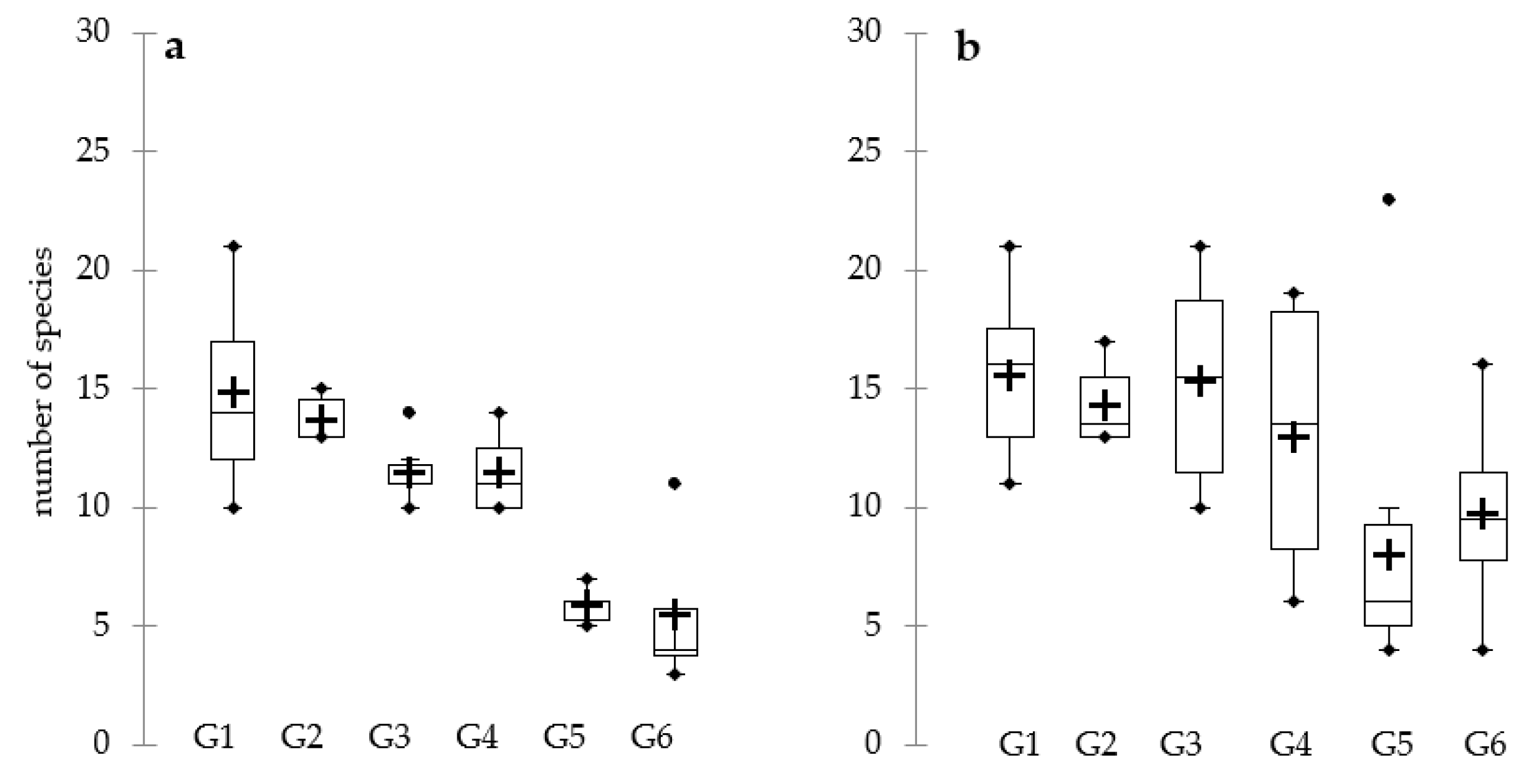
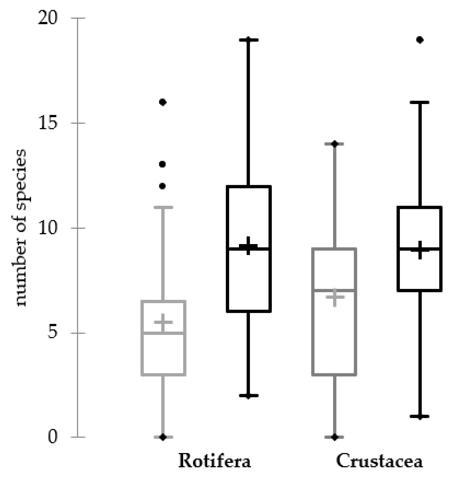
There were significant differences between the harmonic and dystrophic lakes in both the number of crustacean (F = 81.2; p < 0.0001) and rotifer species (F = 19.4; p < 0.0001). The number of crustacean and rotifer species in harmonic lakes was 11–15 and 13–16, respectively, while in dystrophic lakes there were 5–6 and 8–10 species, respectively (Figure 3). However, there was one outlier in the dystrophic lakes (Lake Wądołek, no 38) where 23 Rotifera species were found, and this was the highest number of rotifer species observed in any of the lakes (Figure 3b). The highest diversity of crustacean zooplankton (21 species) was found in oligotrophic Lake Serwy (no. 3). A relatively high number of crustacean species (19) was found in two other oligotrophic lakes (no. 2 and 4).
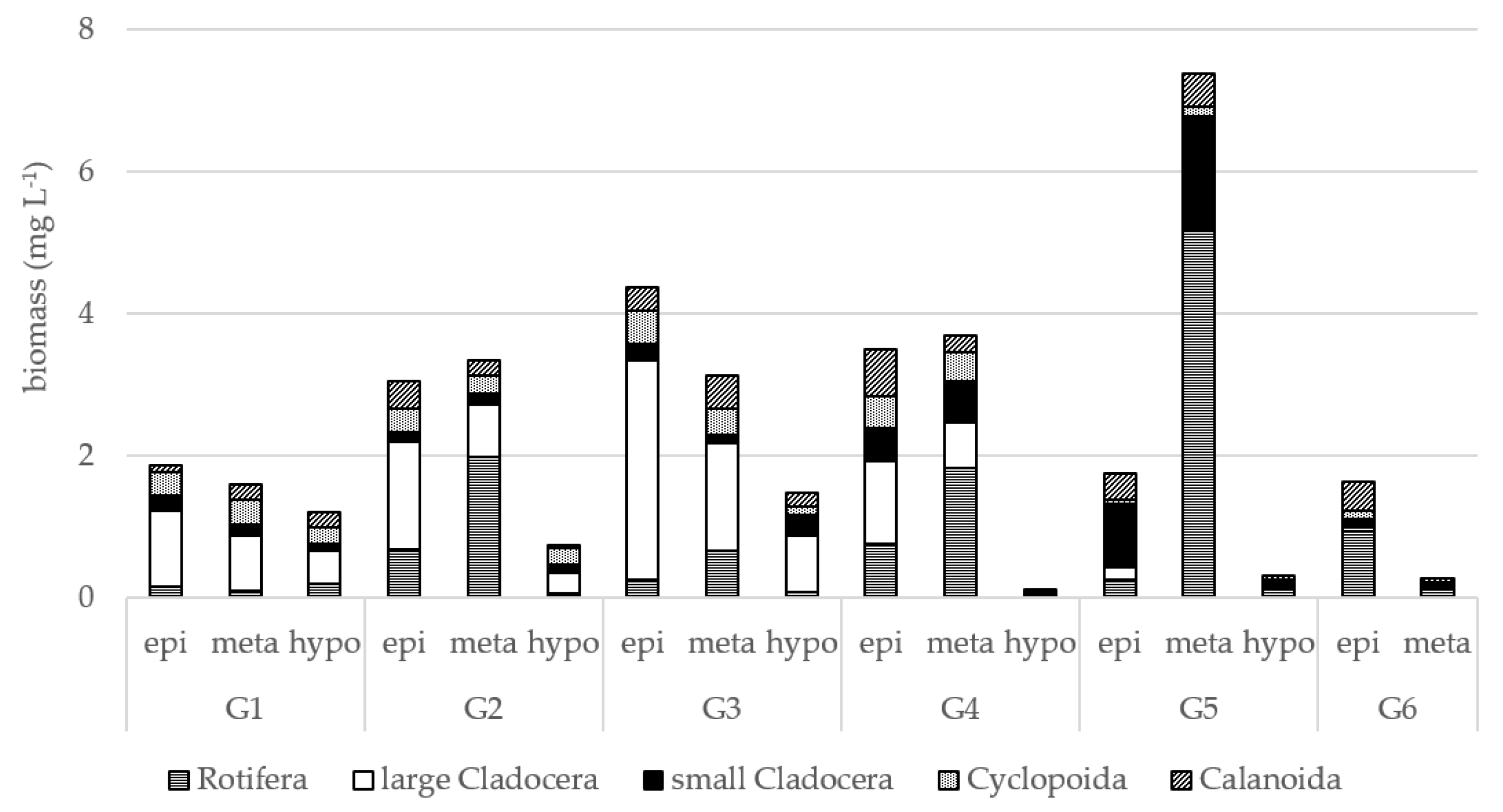
The average biomass of zooplankton in harmonic lakes was 2.3 ± 2.1 mg L−1. The lakes from groups G2–G4 were characterized by a high biomass of zooplankton in the epilimnion and metalimnion, but a low biomass in the hypolimnion. The lakes from G1 were characterized by similar levels of zooplankton biomass in all three layers (Figure 4). The average biomass of zooplankton in dystrophic lakes was 2.7 ± 7.7 mg L−1. The high variability in zooplankton biomass in dystrophic lakes was due to Asplanchna priodonta in two lakes, with biomass reaching 40 mg L−1 (lake no. 31, metalimnion). The low biomass of zooplankton in humic lakes was observed in the hypolimnion of G5 and metalimnion of G6 (Figure 4). The dominant group of zooplankton in harmonic lakes was large Cladocera, except the hypolimnion of G4 lakes, where large Cladocera were almost absent (Figure 4). The large Cladocera in the epilimnion of lakes from G1, G2, and G3 were strongly dominated by Daphnia cucullata and Diaphanosoma brachyurum, but Daphnia cristata and Daphnia longispina increased in the lower layers. The lakes from G2 and G4 were distinguished by a higher relative abundance of Rotifera, and the G4 lakes had an increased share of small Cladocera with a declining share of large Cladocera. The dystrophic lakes were characterized by Rotifera and small Cladocera, and by the low relative abundance of large Cladocera (Figure 4). The most common species with the highest biomass in dystrophic lakes were Asplanchna priodonta, Ceriodaphnia quadrangular, and Eudiaptomus gracilis.
The first axis of the CCA ordination was the most important, contributing to 70.43% of the inertia, and represented the difference between the zooplankton communities in dystrophic lakes (positively related to F1) and harmonic lakes (negatively related to F1). The CCA analysis also distinguished zooplankton communities in the lakes from G1 and G5 (Figure 5). The lakes from G1 were differentiated by the higher share of Daphnia cristata, Daphnia longispina, Bosmina crassicornis, Polyarthra vulgaris, and by species that were classified as glacial relicts. The glacial relicts were found in 11 lakes, mostly from G1, and in one lake from G2 (no. 18). The glacial relicts included Daphnia longiremis (no. 9), Bythotrephes brevimanus (no. 1, 3, 4, 5, 9, 10, and 18), Cyclops lacustris (no. 2, 4, and 9), Eurytemora lacustris (no. 1, 2, 3, 9, 11, and 25) and Heterocope appendiculata (no. 1, 3, 4, 8, 9, and 10). In some lakes, these species were a dominant component of zooplankton communities in lower water layers. The lakes from G5 were characterized by Asplanchna priodonta and Ceriodaphnia quadrangula (Figure 5), while zooplankton communities in lakes G2, G3, G4, and G6 were relatively similar (Figure 5). However, G4 and G6 were characterised by a higher relative abundance of Rotifera, while G2 and G3 both had a higher relative abundance of large Cladocera (Figure 5).
Comparing the number of species in oxic and anoxic water layers revealed significant differences in Rotifera (F = 18.5; p < 0.0001) and Crustacea (F = 10.7; p = 0.001). Anoxic water had fewer rotifers and crustacean species (Figure 6). However, in the case of Crustacea, these differences were smaller due to the relatively high number of species in anoxic conditions (Figure 6).
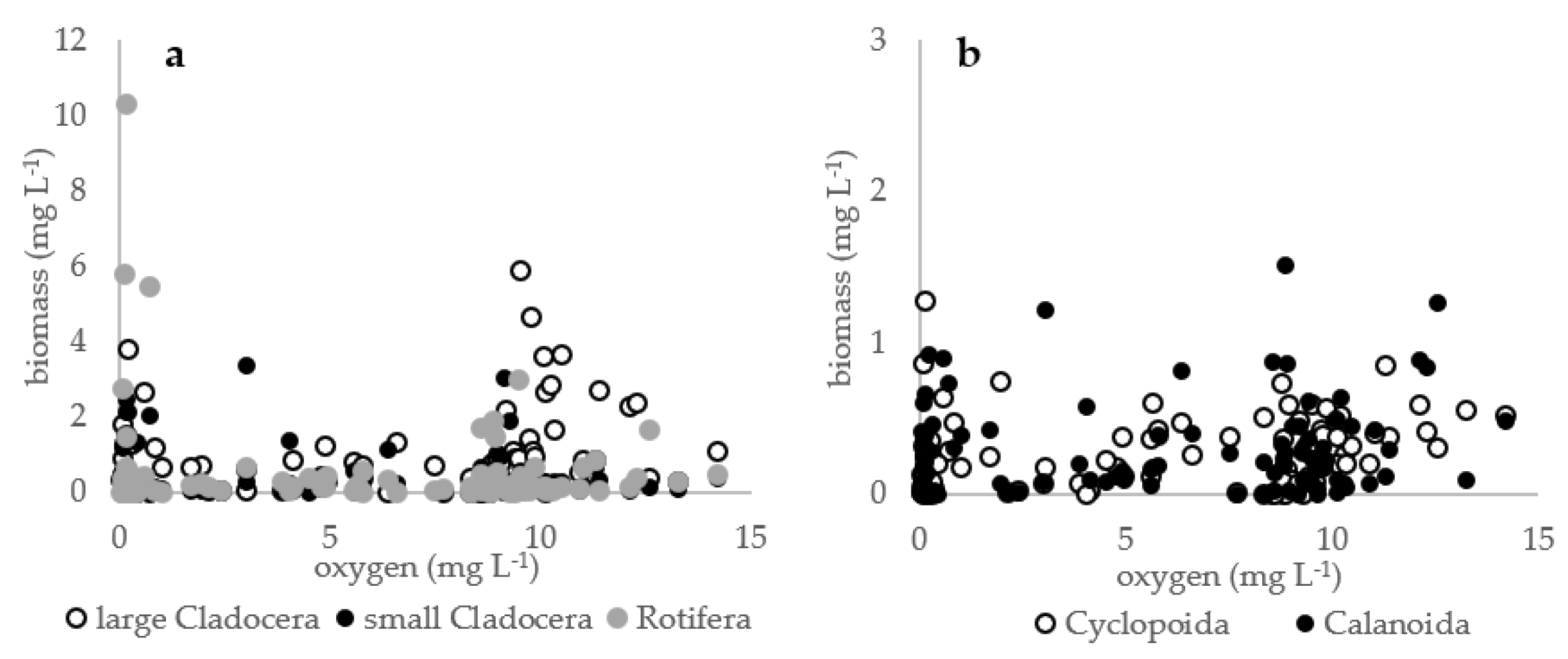
Oxygen concentrations significantly affected the biomass of large Cladocera (F = 10.3; p = 0.002), which reached the highest biomass at high oxygen concentrations (>8 mg L−1). However, a high biomass of large Cladocera was also noted at low oxygen levels (0.1–1 mg L−1). The biomass of Rotifera was not affected by oxygen concentrations (F = 0.7; p = 0.39), but the highest biomass was observed in low oxygen conditions (Figure 7a). The biomass of Rotifera was similar to large Cladocera and also had two peaks at low and high levels of oxygen (Figure 7a). The biomass of small Cladocera was also not affected by oxygen concentrations (F = 0.09; p = 0.74), and high biomass of small Cladocera was observed in different oxygen levels (Figure 7a), except the highest oxygen concentrations (>9 mg L−1). Oxygen concentration significantly affect the biomass of Cyclopoida (F = 12.3; p = 0.001) and Calanoida (F = 4.5; p = 0.035). Their biomasses generally increased with higher oxygen concentrations (Figure 7b). However, a high biomass of Cyclopoida and Calanoida was observed at low oxygen levels (Figure 7b).
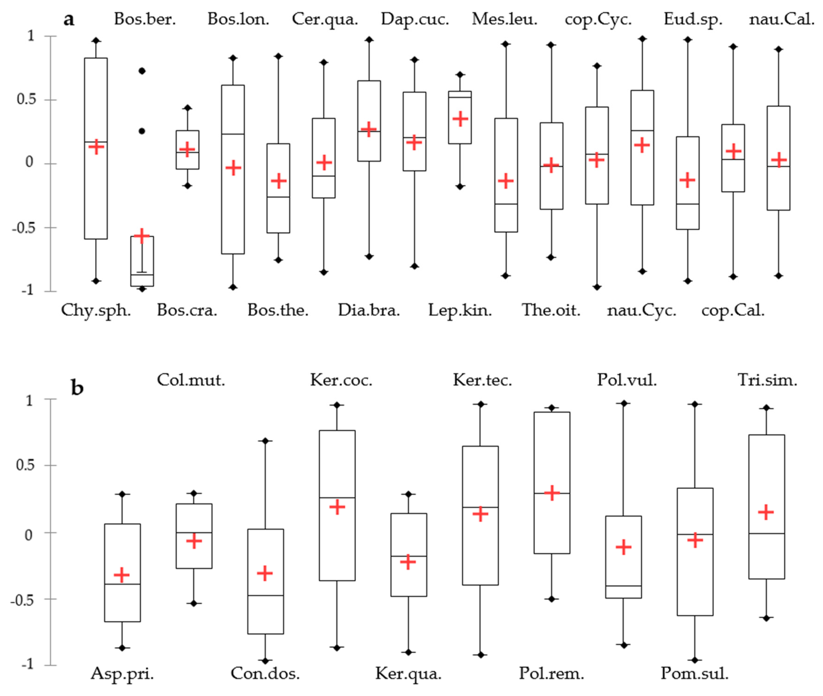
The Habitat Preference Index (HPI) revealed that most of the Cladocera species indicated weak preferences for oxic water layers; however, this also indicated their tolerance for anoxic conditions (Figure 8a). Only Bosmina berolinensis had strong preferences for anoxic conditions. In contrast, Leptodora kindii strongly avoided anoxic conditions. Also, Daphnia cucullata, Bosmina crassicornis and Diaphanosoma brachurum appeared to prefer oxic water layers (Figure 8a), but in the case of the last species, this could also be its preference for higher temperature in the epilimnion. Copepoda taxa showed no clear preferences for oxygen conditions (Figure 8a). Rotifers seemed to be more tolerant of anoxic conditions (Figure 8b) then crustacean species (Figure 8a). The preference for anoxic conditions was indicated for Asplanchna priodonta, Collotheca mutabilis, Conochiloides dossuarius, Keratella quadrata, and Polyarthra vulgaris. No clear preferences were shown for Keratella cochlearis, Keratella tecta, Pompholyx sulcate, and Trichocerca similis. Only Polyarthra remata showed a clear preference for oxic water layers (Figure 8b).
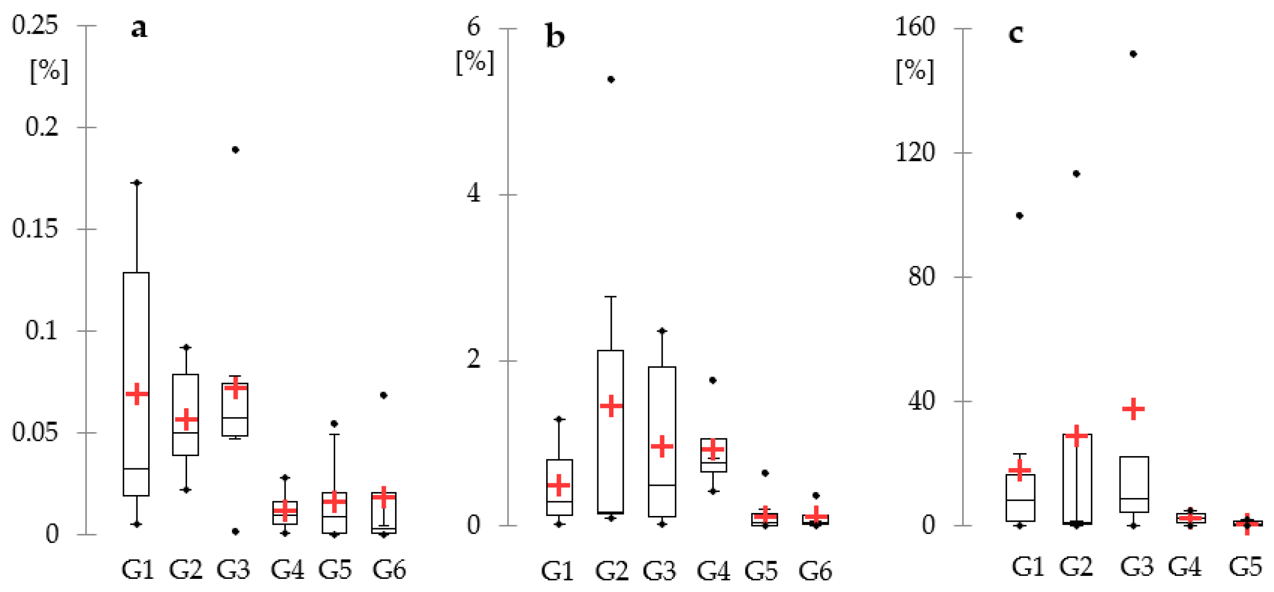
The effectiveness of carbon transfer between phytoplankton and zooplankton increased with depth in all lakes, and the oxygen conditions in each layer were an important factor influencing the transfer of matter in the food web (Figure 9). The effectiveness of carbon transfer in the epilimnion ranged from 0.00004% to 0.19%, with an average of 0.044%. There were also significant differences between the groups G1–G3 and G4–G6 in (F = 14.2; p = 0.001) the epilimnion (Figure 9a). The effectiveness of carbon transfer in the metalimnion ranged from 0.0026% to 5.37%, with an average of 0.64%. There were also significant differences between the groups G1–G4 and G5–G6 (F = 5.5; p = 0.024) in the metalimnion (Figure 9b). The average effectiveness in the metalimnion of G1–G4 was 0.89%, while it was 0.13% in G5–G6. The highest effectiveness of carbon transfer between phytoplankton and zooplankton was in the hypolimnion, and ranged from 0.007% to 151.84%, with an average of 18.26%. There were also differences between the groups G1–G3 and G4–G5 (F = 4.4; p = 0.041) in the hypolimnion (Figure 9c). The average effectiveness in the hypolimnion of G1–G3 was 25.4%, while it was 1.28% in G4–G5.
4. Discussion
Our study provides valuable insight into the role that oxygen stress plays in altering zooplankton communities and carbon transfer in planktonic food webs under different trophic conditions. Freshwater zooplankton in the study lakes were relatively tolerant of anoxic conditions, and large changes in community structure were only found in lakes with the greatest oxygen deficits. The first response of zooplankton to oxygen depletion that we observed was reduced biomass in lower water layers, but generally not in the layer where oxygen deficits began, i.e., in the anoxic metalimnion. We observed even higher biomass of zooplankton in anoxic metalimnia, although warmer waters where the oxygen solubility is lower and the oxygen demand (respiration) is higher [9].
The second response of zooplankton that we observed was a switch in dominance from large to small species. Large Cladocera were the dominant component of zooplankton in lakes with oxic conditions (G1–G3), while in lakes with large oxygen depletion (G4–G6) Rotifera and small Cladocera were the dominant component of the zooplankton communities. The switch from large to small Cladocera could be connected with a higher trophic status and with the dominance of inedible algae or cyanobacteria. Large-bodied cladocerans dominated in low trophic level lakes and oxic conditions because they are better competitors for food than small-bodied species [53,54,55]. However, larger cladocerans experienced difficulty feeding in the presence of cyanobacteria because they do not feed selectively, and longer algae filaments clog their filtering apparatuses [56,57,58,59]. The mass development of inedible algae Gonyostomum semen is a common phenomenon in humic lakes in NE Poland [15,60,61], and the lakes from G4 were eutrophic and dominated by cyanobacteria.
Therefore, inedible algae or cyanobacteria could be the main factor that favors small zooplankton species in these lakes because they are better competitors than large herbivorous filter-feeders in the presence of large inedible algae [62]. However, the dominance of Rotifera and small Cladocera could also be a result of oxygen stress, which may increase the presence and dominance of these taxa in zooplankton communities that are less sensitive to hypoxic conditions [2]. This is consistent with our results, which showed that most rotifers seemed to prefer low oxygen conditions, and the smaller Cladocera were more resistant to oxygen depletion than the larger daphnids. The results from field studies also suggest that decreased meta- and hypolimnetic oxygen concentrations resulted in a shift in zooplankton from large to smaller species [14,18,19]. We observed a similar pattern of changes in zooplankton community structure as a result of oxygen stress, regardless of trophic status, which indicated that oxygen stress is one of the most important factors altering zooplankton structures.
Rotifers are generally more resistant to oxygen deficits than crustaceans [63,64], and laboratory experiments have shown that hypoxia extends the lifespan of rotifers [65]. The results of our study confirm that rotifers are more tolerant of anoxic conditions. Additionally, we found that the greatest biomass of rotifers was observed in anoxic conditions, which suggests that they may have a competitive advantage over crustaceans. Rotifers are often suppressed by large Daphnia both through exploitative competition for shared and limited food resources, as well as through mechanical interference [66,67]. The results from more than 500 freshwater Swedish localities also confirmed that many rotifer species can tolerate hypoxic and anoxic conditions. For example, Polyarthra vulgaris, P. remata, P. major, Asplanchna priodonta, and Kellicottia longispina can tolerate oxygen conditions close to 0 mg L−1, although their maximum abundance occurred at high oxygen concentrations [68,69].
This contrasts with our study where the maximum biomass of Rotifera was found in low oxygen conditions. The information about oxygen preferences for rotifer species is often inconclusive. Elliott (1977) showed that for P. vulgaris the preferable oxygen range was significantly lower than for K. cochlearis [70], which is supported by our results. However, this contrasts with the results from Latvian lakes, where P. vulgaris abundance fluctuated before or after low oxygen conditions [64]. Additional studies on K. cochlearis suggest that this species can tolerate hypoxic waters, but oxygen stress resulted in a smaller body size [71]. Many authors suggest that Asplanchna sp. is sensitive to oxygen limitation [64,70,72], while in our study Asplanchna priodonta had a strong preference for low oxygen conditions. The results of our study clearly indicated that most of the rotifer species could tolerate low oxygen conditions better than microcrustaceans and many of them may reach higher density in hypoxic and anoxic conditions.
Many crustacean species can tolerate DO between 1 and 2 mg L−1, with lethal oxygen concentrations for daphnids and copepods between 0.3 and 1.0 mg L−1 [17,20,73]. Even glacial relicts like the copepod Eurytemora lacustris, which is sensitive to oxygen depletion requires a minimum of 1.0 mg O2 L−1 [74,75]. Laboratory experiments for Daphnia species established a threshold oxygen level at which animals succumbed to oxygen stress at 0.5–1.0 mg L−1 [20]. Crustaceans experience increased metabolic stress in anoxic waters, however, andlow-oxygen tolerance experiments suggest that Daphnia are able to regulate oxygen metabolism across a wide range of DO and produce clones with different amounts of hemoglobin [20]. Other laboratory experiments have shown that crustaceans exhibit reduced survival in anoxic conditions, and mortality can occur within a few hours [17,76,77].
The results from field studies are more ambiguous. Many field observations indicated that the maximum zooplankton density during the day is usually in the top part of the metalimnion with a relatively high oxygen concentration [78,79,80,81]. Other field studies revealed that zooplankton could be found in high abundances in anoxic waters [2,23,82,83]. We observed similar patterns where the upper anoxic layers had a higher biomass of zooplankton and also a large proportion of large Cladocera. Our findings indicate that the upper anoxic layer could be a very important refuge from predation for large species during the day. Studies in marine and freshwater systems have shown that fish are more sensitive to low DO than zooplankton. Most of the freshwater fishes avoid areas where the DO is below 2–4 mg L−1, while the DO below 2 mg L−1 is lethal for most species [11,21,22,84,85]. Although some species of fish developed behavior to dwell for short time periods in the oxygen-deficient meta- and hypolimnion and forage there even in highly hypoxic conditions [32], the results of our study revealed that even large Daphnia could tolerate much lower oxygen concentrations and were often found in the upper anoxic layer. Additionally, our results indicated that the large predatory cladocerans, Leptodora kindii strongly avoid anoxic conditions. We also showed that zooplankton prefers to experience metabolic stress in the anoxic layer during the day to avoid predation.
Zooplankton diversity differed between harmonic and dystrophic lakes. The lowest diversity of crustaceans and rotifers were found in dystrophic lakes. Our previous studies indicated that humic lakes do not offer many niches for zooplankton because of the sharp thermal gradient that results in a shallow layer of oxygenated water [15]. This, together with the high UV radiation in surface waters, limits the distribution of zooplankton to a very narrow water layer [86]. The other limiting factor for zooplankton is the humic stress related to the high content of dissolved organic carbon, humic substances, and low pH [36,87,88]. However, we found a few species that were present only in dystrophic conditions. One of them was Holopedium gibberum, which is widely distributed in water bodies of the boreal zone [89]. This species is rare for the Polish fauna and was noted in softwater lobelia lakes [90]. There is a relatively long list of rotifer species limited in their occurrence to dystrophic lakes, e.g., Keratella paludosa, Lecane acus, Lecane galeata, Lecane elasma, Polyarthra minor, and Microcodon clavus. However, Trichocerca simoneae only recently inhabited Polish dystrophic lakes, and now is among those species achieving the highest densities [91]. This successful invasion is, however, possible only in habitats with a low number of zooplankton species of low density, and dystrophic lakes seem to offer such conditions.
The oxygen deficits in harmonic lakes did not reduce the diversity of Rotifera and Crustacea communities. We found a similar number of species in lakes with different trophic conditions (oligotrophic, mesotrophic, eutrophic), as well as in lakes with different oxygen conditions (G1–G4). Moreover, our results suggest that oxygen deficits in low trophic conditions could even increase the crustacean diversity as they created niches for small-bodied Cladocera. This is an interesting phenomenon as most often the opposite is true, where a well-oxygenated hypolimnion zone promotes a large diversity of crustacean zooplankton due to vertical niche segregation [16,81,92]. Our results also confirm this idea, as most of the lakes without oxygen depletion supported planktonic glacial relicts that have high habitat requirements. We found glacial relicts in 11 lakes, and among them were Daphnia longiremis, Bythotrephes brevimanus, Cyclops lacustris, Eurytemora lacustris, and Heterocope appendiculata.
Our study extends our knowledge about the distribution of planktonic relict species in central Europe. Untill now, we did not know much about glacial relicts in Poland as data only existed from a few lakes that were studied often [16] and a few single records [81,90,93,94] that were available. Consequently, our research has identified many new records, which suggest that glacial relicts are more common in the deep lakes of northern Poland. Another important finding is a revision of the distribution of Bythotrephes in Poland as most previous research from Poland indicated the occurrence of B. longimanus [16,41,81,94,95]. We found that in NE Poland B. brevimanus is the most common species. The geographical distribution of the genus Bythotrephes presented by Litvinchuk and Litvinchuk (2016) and Korovchinsky (2018) confirms our finding [96,97]. The distribution of B. longimanus is more to the north in the boreal zone and also from lakes in the Alps, while the prevalence of B. brevimanus is clear in the north of the European mainland, from the Netherlands to Belarus and the Baltic republics [97,98]. However, a detailed description of this species will be presented in a separate paper.
The results of our study indicate that oxygen stress is an important factor that reduces the effectiveness of matter transfer between phytoplankton and zooplankton. The primary producers convert inorganic carbon into organic carbon, which is incorporated into new zooplankton biomass. Therefore, the productivity and effectiveness of matter transfer are frequently measured in carbon mass units [99,100]. We observed large differences between the primary and secondary production in the water depth layers. Primary production tended to decrease with depth, while zooplankton production in the vertical profile was strongly related to oxygen conditions, resulting in significant differences in the effectiveness of matter transfer between the epilimnion and hypolimnion.
The average effectiveness of carbon transfer from phytoplankton to zooplankton in the epilimnion was 0.044%, which is much lower than the 10% of energy and matter, which is theoretically expected to pass to the next trophic level [101,102]. However, the efficiency increased with depth, with average values of 0.64% in the metalimnion and 18.26% in the hypolimnion. Therefore, a reduction of zooplankton in the lower water layers caused by oxygen stress strongly affects the transfer of energy and matter in the freshwater food webs. This also emphasized the role of glacial relicts in the transfer energy and matter in the lake ecosystem, because they are often a dominant component of the zooplankton in the deep water layers.
Additionally, the lakes with strong oxygen depletion (groups G4–G6) were characterized by a lower effectiveness of transfer of matter in the whole water profile. However, previous data about transfer efficiency are inconsistent. Pauly and Christensen (1995) reported that efficiency in marine ecosystems ranged between 2% and 24% [99]. Lacroix et al. (1999) presented similar values of transfer efficiency between phytoplankton and zooplankton in lakes [103]. Other research with more accurate methods indicated that only 0.1% of the carbon produced by phytoplankton is incorporated into zooplankton [104,105]. Measurements of carbon transfer in algal and bacteria food webs revealed similar low efficiencies for both pathways [106,107]. The cited above data confirm our suggestion that the effectiveness of matter transfer through planktonic freshwater food webs is much lower than the theoretical 10%.
Supplementary Materials
The following are available online at https://www.mdpi.com/2073-4441/12/3/706/s1, Table S1. Frequency (%) of zooplankton taxa occurrence in harmonic and dystrophic lakes with different oxygen conditions (G1–G6).
Author Contributions
M.K. designed the study, undertook field analyses and sampling, analyzed the crustacean zooplankton, performed statistical analysis, and wrote the manuscript; J.E.-K. analyzed the Rotifera zooplankton and reviewed the manuscript; J.K. participated in field and data analysis, worked with glacial relicts; I.F. participated in laboratory analyses and reviewed the manuscript; A.R.D. supervised the research and revised the manuscript. All authors have read and agreed to the published version of the manuscript.
Funding
This research was supported by the Polish National Science Centre by grant number 2017/01/X/NZ8/01151 and 2016/21/B/NZ8/00434.
Acknowledgments
The authors are thankful to the employees of the Wigry National Park for their help in the collection of samples and to Adam Więcko and Helena Samsonowicz for their assistance in the water chemistry analyses.
Conflicts of Interest
The authors declare no conflict of interest.
References
- Ekau, W.; Auel, H.; Pörtner, H.-O.; Gilbert, D. Impacts of hypoxia on the structure and processes in pelagic communities (zooplankton, macro-invertebrates and fish). Biogeosciences 2010, 7, 1669–1699. [Google Scholar] [CrossRef] [Green Version]
- Doubek, J.P.; Campbell, K.L.; Lofton, M.E.; McClure, R.P.; Carey, C.C. Hypolimnetic Hypoxia Increases the Biomass Variability and Compositional Variability of Crustacean Zooplankton Communities. Water 2019, 11, 2179. [Google Scholar] [CrossRef] [Green Version]
- Górniak, A.; Kajak, Z. Hydrobiologia. Limnologia; Wydawnictwo Naukowe PWN: Warszawa, Poland, 2019; pp. 45–108. ISBN 978-83-01-20721-2. (In Polish) [Google Scholar]
- Winder, M.; Schindler, D.E. Climatic effects on the phenology of lake processes. Glob. Chang. Boil. 2004, 10, 1844–1856. [Google Scholar] [CrossRef] [Green Version]
- Jankowski, T.; Livingstone, D.M.; Bührer, H.; Forster, R.; Niederhauser, P. Consequences of the 2003 European heat wave for lake temperature profiles, thermal stability, and hypolimnetic oxygen depletion: Implications for a warmer world. Limnol. Oceanogr. 2006, 51, 815–819. [Google Scholar] [CrossRef] [Green Version]
- Butcher, J.B.; Nover, D.; Johnson, T.E.; Clark, C.M. Sensitivity of lake thermal and mixing dynamics to climate change. Clim. Chang. 2015, 129, 295–305. [Google Scholar] [CrossRef] [Green Version]
- Diaz, R.J.; Rosenberg, R. Spreading dead zones and consequences for marine ecosystems. Science 2008, 321, 926–929. [Google Scholar] [CrossRef]
- Jenny, J.P.; Francus, P.; Normandeau, A.; Lapointe, F.; Perga, M.E.; Ojala, A.; Schimmelmann, A.; Zolitschka, B. Global spread of hypoxia in freshwater ecosystems during the last three centuries is caused by rising local human pressure. Glob. Chang. Biol. 2016, 22, 1481–1489. [Google Scholar] [CrossRef]
- Doubek, J.P.; Campbell, K.L.; Doubek, K.M.; Hamre, K.D.; Lofton, M.E.; McClure, R.P.; Ward, N.K.; Carey, C.C. The effects of hypolimnetic anoxia on the diel vertical migration of freshwater crustacean zooplankton. Ecosphere 2018, 9, e02332. [Google Scholar] [CrossRef] [Green Version]
- Kolar, C.S.; Rahel, F.J. Interaction of a biotic factor (predator presence) and an abiotic factor (low oxygen) as an influence on benthic invertebrate communities. Oecologia 1993, 95, 210–219. [Google Scholar] [CrossRef]
- Ludsin, S.A.; Zhang, X.; Brandt, S.B.; Roman, M.R.; Boicourt, W.C.; Mason, D.M.; Costantini, M. Hypoxia-avoidance by planktivorous fish in Chesapeake Bay: Implications for food web interactions and fish recruitment. J. Exp. Mar. Boil. Ecol. 2009, 381, S121–S131. [Google Scholar] [CrossRef]
- Miller, D.; Poucher, S.; Coiro, L.L. Determination of lethal dissolved oxygen levels for selected marine and estuarine fishes, crustaceans, and a bivalve. Mar. Biol. 2002, 140, 287–296. [Google Scholar] [CrossRef]
- Vaquer-Sunyer, R.; Duarte, C.M. Thresholds of hypoxia for marine biodiversity. Proc. Natl. Acad. Sci. USA 2008, 105, 15452–15457. [Google Scholar] [CrossRef] [PubMed] [Green Version]
- Chang, K.H.; Imai, H.; Ayukawa, K.; Sugahara, S.; Nakano, S.I.; Seike, Y. Impact of improved bottom hypoxia on zooplankton community in shallow eutrophic lake. Knowl. Manag. Aquat. Ecosyst. 2013, 408, 1–8. [Google Scholar] [CrossRef]
- Karpowicz, M.; Ejsmont-Karabin, J. Influence of environmental factors on vertical distribution of zooplankton communities in humic lakes. Ann. Limnol. Int. J. Limnol. 2018, 54, 17. [Google Scholar] [CrossRef]
- Karpowicz, M.; Ejsmont-Karabin, J.; Więcko, A.; Górniak, A.; Cudowski, A. A place in space - the horizontal vs. vertical factors that influence zooplankton (Rotifera, Crustacea) communities in a mesotrophic lake. J. Limnol. 2019, 78, 243–258. [Google Scholar] [CrossRef]
- Stalder, L.C.; Marcus, N.H. Zooplankton responses to hypoxia: Behavioral patterns and survival of three species of calanoid copepods. Mar. Biol. 1997, 127, 599–607. [Google Scholar] [CrossRef]
- Wright, D.; Shapiro, J. Refuge availability: A key to understanding the summer disappearance of Daphnia. Freshw. Biol. 1990, 24, 43–62. [Google Scholar] [CrossRef]
- Field, K.M.; Prepas, E.E. Increased abundance and depth distribution of pelagic crustacean zooplankton during hypolimnetic oxygenation in a deep, eutrophic Alberta lake. Can. J. Fish. Aquat. Sci. 1997, 54, 2146–2156. [Google Scholar] [CrossRef]
- Weider, L.J.; Lampert, W. Differential response of Daphnia genotypes to oxygen stress: Respiration rates, hemoglobin content and low-oxygen tolerance. Oecologia 1985, 65, 487–491. [Google Scholar] [CrossRef]
- Klumb, R.A.; Bunch, K.L.; Mills, E.L.; Rudstam, L.G.; Brown, G.; Knauf, C.; Burton, R.; Arrhenius, F. Establishment of a metalimnetic oxygen refuge for zooplankton in a productive Lake Ontario embayment. Ecol. Appl. 2004, 14, 113–131. [Google Scholar] [CrossRef]
- Stanley, D.R.; Wilson, C.A. Effect of hypoxia on the distribution of fishes associated with a petroleum platform off coastal Louisiana. N. Am. J. Fish. Manag. 2004, 24, 662–671. [Google Scholar] [CrossRef]
- Vanderploeg, H.A.; Ludsin, S.A.; Cavaletto, J.F.; Höök, T.O.; Pothoven, S.A.; Brandt, S.B.; Liebig, J.R.; Lang, G.A. Hypoxic zones as habitat for zooplankton in Lake Erie: Refuges from predation or exclusions zones? J. Exp. Mar. Biol. Ecol. 2009, 381, 108–120. [Google Scholar] [CrossRef]
- Vanderploeg, H.A.; Ludsin, S.A.; Ruberg, S.A.; Hook, T.O.; Pothoven, S.A.; Brandt, S.B.; Lang, G.A.; Liebig, J.R. Hypoxia affects spatial distributions and overlap of pelagic fish, zooplankton, and phytoplankton in Lake Erie. J. Exp. Mar. Biol. Ecol. 2009, 381, 92–107. [Google Scholar] [CrossRef]
- Larsson, P.; Lampert, W. Experimental evidence of a low oxygen refuge for large zooplankton. Limnol. Oceanogr. 2011, 56, 1682–1688. [Google Scholar] [CrossRef]
- Karpowicz, M.; Ejsmont-Karabin, J. Effect of metalimnetic gradient on phytoplankton and zooplankton (Rotifera, Crustacea) communities in different trophic conditions. Environ. Monit. Assess. 2017, 189, 367. [Google Scholar] [CrossRef] [PubMed] [Green Version]
- Karpowicz, M.; Kalinowska, K. Vertical distribution of the relic species Eurytemora lacustris (Copepoda, Calanoida) in stratified mesotrophic lakes. Biologia 2018, 73, 1197–1204. [Google Scholar] [CrossRef] [PubMed] [Green Version]
- Kobayashi, M.; Hoshi, T. Analysis of respiratory role of haemoglobin in Daphnia magna. Zool. Sci. 1984, 1, 523–532. [Google Scholar]
- Hanazato, T.; Dodson, S.I. Synergistic effects of low oxygen concentration, predator kairomone, and a pesticide on the cladoceran Daphnia pulex. Limnol. Oceanogr. 1995, 40, 700–709. [Google Scholar] [CrossRef]
- Larsson, P.; Lampert, W. Finding the optimal vertical distribution: Behavioural responses of Daphnia pulicaria to gradients of environmental factors and the presence of fish. Freshw. Biol. 2012, 57, 2514–2525. [Google Scholar] [CrossRef]
- Wilczyński, W.; Dynak, P.; Babkiewicz, E.; Bernatowicz, P.; Maszczyk, P. The combined effects of hypoxia and fish kairomones on several physiological and life history traits of Daphnia. Freshw. Biol. 2019, 64, 2204–2220. [Google Scholar] [CrossRef]
- Maszczyk, P.; Babkiewicz, E.; Ciszewski, K.; Dabrowski, K.; Dynak, P.; Krajewski, K.; Urban, P.; Żebrowski, M.; Wilczynski, W. Combined effects of elevated epilimnetic temperature and metalimnetic hypoxia on the predation rate of planktivorous fish. J. Plankton Res. 2019, 41, 709–722. [Google Scholar] [CrossRef] [PubMed]
- Sorensen, M.L.; Branstrator, D.K. The North American invasive zooplanktivore Bythotrephes longimanus is less hypoxia-tolerant than the native Leptodora kindtii. Can. J. Fish. Aquat. Sci. 2017, 74, 824–832. [Google Scholar] [CrossRef] [Green Version]
- Berzins, B.; Pejler, B. Rotifer occurrence in relation to oxygen content. Hydrobiologia 1989, 183, 165–172. [Google Scholar] [CrossRef]
- Jekatierynczuk-Rudczyk, E.; Zieliński, P.; Grabowska, M.; Ejsmont-Karabin, J.; Karpowicz, M.; Więcko, A. The trophic status of Suwałki Landscape Park lakes based on selected parameters (NE Poland). Environ. Monit. Assess. 2014, 186, 5101–5121. [Google Scholar] [CrossRef] [PubMed] [Green Version]
- Górniak, A. A new version of the Hydrochemical Dystrophy Index to evaluate dystrophy in lakes. Ecol. Indic. 2017, 78, 566–573. [Google Scholar] [CrossRef]
- Carlson, R.E. A trophic state index for lakes. Limnol. Oceanogr. 1977, 22, 361–369. [Google Scholar] [CrossRef] [Green Version]
- Drzymulska, D.; Zieliński, P. Developmental changes in the historical and present-day trophic status of brown water lakes. Are humic water bodies a uniform aquatic ecosystem? Wetlands 2013, 33, 909–919. [Google Scholar] [CrossRef] [Green Version]
- Kring, S.A.; Figary, S.E.; Boyer, G.L.; Watson, S.B.; Twiss, M.R. Rapid in situ measures of phytoplankton communities using the bbe FluoroProbe: Evaluation of spectral calibration, instrument intercompatibility, and performance range. Can. J. Fish. Aquat. Sci. 2014, 71, 1087–1095. [Google Scholar] [CrossRef]
- Neal, C.; Neal, M.; Wickham, H. Phosphate measurement in natural waters: Two examples of analytical problems associated with silica interference using phosphomolybdic acid methodologies. Sci. Total Environ. 2000, 251–252, 513–542. [Google Scholar] [CrossRef]
- Błędzki, L.A.; Rybak, J.I. Freshwater Crustacean Zooplankton of Europe; Springer: Cham, Switzerland, 2016; pp. 1–918. [Google Scholar] [CrossRef]
- Ejsmont-Karabin, J. Empirical equations for biomass calculation of planktonic rotifers. Pol. Arch. Hydrobiol. 1998, 45, 513–522. [Google Scholar]
- Hart, R.C.; Bychek, E.A. Body size in freshwater planktonic crustaceans: An overview of extrinsic determinants and modifying influences of biotic interactions. Hydrobiologia 2011, 668, 61–108. [Google Scholar] [CrossRef]
- Feniova, I.; Dawidowicz, P.; Ejsmont-Karabin, J.; Gladyshev, M.I.; Kalinowska, K.; Karpowicz, M.; Kostrzewska-Szlakowska, I.; Majsak, N.; Petrosyan, V.; Razlutskij, V.; et al. Effects of zebra mussels on cladoceran communities under eutrophic conditions. Hydrobiologia 2018, 822, 37–54. [Google Scholar] [CrossRef] [Green Version]
- Karpowicz, M.; Feniova, I.; Gladyshev, M.I.; Ejsmont-Karabin, J.; Górniak, A.; Zieliński, P.; Dawidowicz, P.; Kolmakova, A.A.; Dzialowski, A.R. The stoichiometric ratios (C:N:P) in a pelagic food web under experimental conditions. Limnologica 2019, 77, 125690. [Google Scholar] [CrossRef] [Green Version]
- Ivlev, V.S. Experimental Ecology of the Feeding of Fishes; Yale University Press: New Haven, CT, USA, 1961; pp. 1–302. [Google Scholar]
- Gaevsky, N.A.; Kolmakov, V.I.; Popelnitsky, V.A.; Gold, V.M.; Dubovskaya, O.P. Evaluation of the effect of light intensity on the measurement of the photosynthetic rate in plankton microalgae by the chlorophyll fluorescence method. Russ. J. Plant Physiol. 2000, 47, 820–825. [Google Scholar] [CrossRef]
- Ishimaru, T.; Mimuro, M.; Fujita, Y. Estimation of phytoplankton photosynthesis using a fluorescence induction technique. J. Plankton Res. 1985, 7, 679–689. [Google Scholar] [CrossRef]
- Alimov, A.F. An Introduction to Production Hydrobiology; Gidrometeoizdat: Leningrad, Russia, 1989; pp. 1–152. [Google Scholar]
- Stockwell, J.D.; Johansson, O.E. Temperature-dependent allometric models to estimate zooplankton production in temperate freshwater lakes. Can. J. Fish. Aquat. Sci. 1997, 54, 2350–2360. [Google Scholar] [CrossRef]
- Bottrell, H.H.; Duncan, A.; Gliwicz, Z.M.; Grygierek, E.; Herzig, A.; Hillbricht-Ilkowska, A.; Kurasawa, H.; Larsson, P.; Węgleńska, T. A review of some problems in zooplankton production studies. Nor. J. Zool. 1976, 24, 419–456. [Google Scholar]
- Ter Braak, C.J.F. Canonical correspondence analysis: A new eigenvector technique for multivariate direct gradient analysis. Ecology 1986, 67, 1167–1179. [Google Scholar] [CrossRef] [Green Version]
- Brooks, J.L.; Dodson, S.I. Predation, body size and composition of plankton. Science 1965, 150, 28–35. [Google Scholar] [CrossRef]
- Gliwicz, Z.M. Between Hazards of Starvation and Risk of Predation: The Ecology of Off-Shore Animals; International Ecology Institute: Oldendorf (Luhe), Germany, 2003; ISBN 978-3-946729-12-9. [Google Scholar]
- Sikora, A.; Dawidowicz, P. Do the presence of filamentous cyanobacteria and an elevated temperature favor small-bodied Daphnia in interspecific competitive interactions? Fundam. Appl. Limnol. 2014, 185, 307–314. [Google Scholar] [CrossRef]
- Henning, M.; Hertel, W.; Wall, H.; Kohl, J.G. Strain-specific influence of Microcystis aeruginosa on food ingestion and assimilation of some cladocerans and copepods. Int. Rev. Ges. Hydrobiol. 1991, 76, 37–45. [Google Scholar] [CrossRef]
- Mayer, J.; Dokulil, M.T.; Salbrechter, M.; Berger, M.; Posch, T.; Pfister, G.; Kirschner, A.K.T.; Velimorov, B.; Steitz, A.; Ulbricht, T. Seasonal succession and trophic relations between phytoplankton, zooplankton, ciliate and bacteria in a hypertrophic shallow lake in Vienna, Austria. Hydrobiologia 1997, 342–343, 165–174. [Google Scholar] [CrossRef]
- Cyr, H. Cladoceran- and copepod-dominated zooplankton communities graze at similar rates in low-productivity lakes. Can. J. Fish. Aquat. Sci. 1998, 55, 414–422. [Google Scholar] [CrossRef]
- Górniak, A.; Karpowicz, M. Development of crustacean plankton in a shallow, polyhumic reservoir in the first 20 years after impoundment (northeast Poland). Inland Waters 2014, 4, 311–318. [Google Scholar] [CrossRef]
- Hutorowicz, A.; Szeląg-Wasielewska, E.; Grabowska, M.; Owsianny, P.M.; Pęczuła, W.; Luscińska, M. The occurrence of Gonyostomum semen (Raphidophyceae) in Poland. Flor. Geobot. Pol. 2006, 13, 399–407. [Google Scholar]
- Pęczuła, W.; Grabowska, M.; Zieliński, P.; Karpowicz, M.; Danilczyk, M. Vertical distribution of expansive, bloom-forming algae Gonyostomum semen vs. plankton community and water chemistry in four small humic lakes. Knowl. Manag. Aquat. Ecosyst. 2018, 419, 28. [Google Scholar] [CrossRef]
- DeMott, W.R.; Kerfoot, W.C. Competition among cladocerans: Nature of the interactions between Bosmina and Daphnia. Ecology 1982, 6, 1949–1966. [Google Scholar] [CrossRef]
- Esparcia, A.; Miracle, M.R.; Serra, M. Brachionus plicatilis tolerance to low oxygen concentrations. Hydrobiologia 1989, 186, 331–337. [Google Scholar] [CrossRef]
- Dimante-Deimantovica, I.; Skute, A.; Skute, R. Vertical variability of pelagic zooplankton fauna in deep Latvian lakes, with some notes on changes in ecological conditions. Est. J. Ecol. 2012, 61, 247–264. [Google Scholar] [CrossRef] [Green Version]
- Snell, T.W.; Johnston, R.K.; Jones, B.L. Hypoxia extends lifespan of Brachionus manjavacas (Rotifera). Limnetica 2019, 38, 159–166. [Google Scholar] [CrossRef]
- Gilbert, J.J. Suppression of rotifer populations by Daphnia: A review of the evidence, the mechanisms, and the effects on zooplankton community structure. Limnol. Oceanogr. 1988, 33, 1286–1303. [Google Scholar] [CrossRef]
- Gilbert, J.J. Susceptibilities of ten rotifer species to interference from Daphnia pulex. Ecology 1988, 69, 1826–1838. [Google Scholar] [CrossRef]
- Kizito, Y.S.; Nauwerck, A. Temporal and vertical distribution of planktonic rotifers in a meromictic crater lake, Lake Nyahirya (Western Uganda). Hydrobiologia 1995, 312–314, 303–312. [Google Scholar] [CrossRef]
- Bertilsson, J.; Berzins, B.; Pejler, B. Occurrence of limnic micro-crustaceans in relation to temperature and oxygen. Hydrobiologia 1995, 299, 163–167. [Google Scholar] [CrossRef]
- Elliott, J.I. Seasonal changes in the abundance and distribution of planktonic rotifers in Grasmere (English Lake District). Freshw. Biol. 1977, 7, 147–166. [Google Scholar] [CrossRef]
- Czarnoleski, M.; Ejsmont-Karabin, J.; Angilletta, M.J., Jr.; Kozlowski, J. Colder rotifers grow larger but only in oxygenated waters. Ecosphere 2015, 6, 1–5. [Google Scholar] [CrossRef]
- Mikschi, E. Rotifer distribution in relation to temperature and oxygen content. Hydrobiologia 1989, 186–187, 209–214. [Google Scholar] [CrossRef]
- Lass, S.; Boersma, M.; Spaak, P. How do migrating daphnids cope with fish predation risk in the epilimnion under anoxic conditions in the hypolimnion? J. Plankton Res. 2000, 22, 1411–1418. [Google Scholar] [CrossRef]
- Kasprzak, P.; Reese, C.; Koschel, R.; Schulz, M.; Hambaryan, I.; Mathes, J. Habitat characteristics of Eurytemora lacustris (Poppe, 1887) (Copepoda, Calanoida): The role of lake depth, temperature, oxygen concentration and light intensity. Int. Rev. Hydrobiol. 2005, 90, 292–309. [Google Scholar] [CrossRef]
- Maier, G.; Speth, B.; Wolfgang, A.R.P.; Bahnwart, M.; Kasprzak, P. New records of the rare glacial relict Eurytemora lacustris (Poppe 1887) (Copepoda; Calanoida) in atypical lake habitats of northern Germany. J. Limnol. 2011, 70, 145–148. [Google Scholar] [CrossRef] [Green Version]
- Tinson, S.; Laybourn-Parry, J. The behavioural responses and tolerance of freshwater benthic cyclopoid copepods to hypoxia and anoxia. Hydrobiologia 1985, 127, 257–263. [Google Scholar] [CrossRef]
- Roman, M.R.; Gauzens, A.L.; Rhinehart, W.K.; White, J.R. Effects of low oxygen waters on Chesapeake Bay zooplankton. Limnol. Oceanogr. 1993, 38, 1603–1614. [Google Scholar] [CrossRef]
- Gliwicz, Z.M.; Pijanowska, J. Effects of predation and resource depth distribution on vertical migration of zooplankton. Bull. Mar. Sci. 1988, 43, 695–709. [Google Scholar]
- Loose, C.J.; Dawidowicz, P. Trade-offs in diel vertical migration by zooplankton: The costs of predator avoidance. Ecology 1994, 75, 2255–2263. [Google Scholar] [CrossRef]
- Pannard, A.; Planas, D.; Beisner, B.E. Macrozooplankton and the persistence of the deep chlorophyll maximum in a stratified lake. Freshw. Biol. 2015, 60, 1717–1733. [Google Scholar] [CrossRef]
- Sługocki, Ł.; Czerniawski, R. Trophic state (TSISD) and mixing type significantly influence pelagic zooplankton biodiversity in temperate lakes (NW Poland). PeerJ 2018, 6, e5731. [Google Scholar] [CrossRef] [Green Version]
- Nolan, S.; Bollens, S.M.; Rollwagen-Bollens, G. Diverse taxa of zooplankton inhabit hypoxic waters during both day and night in a temperate eutrophic lake. J. Plankton Res. 2019, 41, 431–447. [Google Scholar] [CrossRef]
- Roman, M.R.; Brandt, S.B.; Houde, E.D.; Pierson, J.J. Interactive Effects of Hypoxia and Temperature on Coastal Pelagic Zooplankton and Fish. Front. Mar. Sci. 2019, 6, 139. [Google Scholar] [CrossRef] [Green Version]
- Suthers, I.M.; Gee, J.H. Role of hypoxia in limiting summer distribution of juvenile yellow perch (Perca flavescens) in a prairie marsh. Can. J. Fish. Aquat. Sci. 1986, 43, 1562–1570. [Google Scholar] [CrossRef]
- Eby, L.A.; Crowder, L.B. Hypoxia-based habitat compression in the Neuse River Estuary: Context-dependent shifts in behavioral avoidance thresholds. Can. J. Fish. Aquat. Sci. 2002, 59, 952–965. [Google Scholar] [CrossRef]
- Rautio, M.; Tartarotti, B. UV radiation and freshwater zooplankton: Damage, protection and recovery. Freshw. Rev. 2010, 3, 105–131. [Google Scholar] [CrossRef] [PubMed] [Green Version]
- Robidoux, M.; del Giorgio, P.; Derry, A. Effects of humic stress on the zooplankton from clear and DOC-rich lakes. Freshw. Biol. 2015, 60, 1263–1278. [Google Scholar] [CrossRef]
- Taipale, S.J.; Vuorio, K.; Strandberg, U.; Kahilainen, K.K.; Järvinen, M.; Hiltunen, M.; Peltomaa, E.; Kankaala, P. Lake eutrophication and brownification downgrade availability and transfer of essential fatty acids for human consumption. Environ. Int. 2016, 96, 156–166. [Google Scholar] [CrossRef] [PubMed] [Green Version]
- Podshivalina, V.N.; Sheveleva, N.G.; Bayanov, N. Biology and Ecology of Holopedium gibberum (Branchiopoda: Cladocera: Ctenopoda) in the Palearctic. Hydrobiol. J. 2012, 48, 28–36. [Google Scholar] [CrossRef]
- Kuczyńska-Kippen, N.; Klimaszyk, P.; Piotrowicz, R. Zooplankton communities in three adjacent softwater lobelia lakes of slightly differentiated morphology and trophic state. Limnol. Rev. 2017, 17, 207–214. [Google Scholar] [CrossRef]
- Ejsmont-Karabin, J. Rotifer invasion? On appearance and abundance of tropical species in lakes of North-Eastern Poland. Pol. J. Ecol. 2014, 62, 727–733. [Google Scholar] [CrossRef]
- Brzeziński, T.; Fronk, J.; Trzcińska-Danielewicz, J.; Dawidowicz, P. Interspecific hybridization in sympatric species of Daphnia inhabiting lakes in north-eastern Poland. Oceanol. Hydrobiol. Stud. 2012, 41, 1–6. [Google Scholar] [CrossRef]
- Sługocki, Ł.; Rymaszewska, A.; Kirczuk, L. Insights into the morphology and molecular characterization of glacial relict Eurytemora lacustris (Poppe, 1887) (Crustacea, Copepoda, Calanoida, Temoridae). ZooKeys 2019, 864, 15–33. [Google Scholar] [CrossRef]
- Ejsmont-Karabin, J.; Kalinowska, K.; Karpowicz, M. Structure of Ciliate, Rotifer, and Crustacean Communities in Lake Systems of Northeastern Poland. In Polish River Basins and Lakes—Part II; Springer: Cham, Switzerland, 2020; Volume 87, pp. 77–101. [Google Scholar] [CrossRef]
- Rybak, J.I.; Błędzki, L.A. Słodkowodne Skorupiaki Planktonowe. Klucz do Oznaczania Gatunków; Wydawnictwa Uniwersytetu: Warszawskiego, Poland, 2010; (In Polish). [Google Scholar] [CrossRef]
- Litvinchuk, L.F.; Litvinchuk, S.N. Morphological diversity and widespread hybridization in the genus Bythotrephes Leydig, 1860 (Branchiopoda, Onychopoda, Cercopagidae). Arch. Biol. Sci. 2016, 68, 67–79. [Google Scholar] [CrossRef]
- Korovchinsky, N.M. Further revision of the genus Bythotrephes Leydig (Crustacea: Cladocera: Onychopoda): Redescription of B. brevimanus Lilljeborg, reevaluation of B. cederströmii Schödler, and description of a new species of the genus. Zootaxa 2018, 4379, 347–387. [Google Scholar] [CrossRef]
- Korovchinsky, N.M. Morphological assessment of the North Eurasian interspecific hybrid forms of the genus Bythotrephes Leydig, 1860 (Crustacea: Cladocera: Cercopagididae). Zootaxa 2019, 4550, 340–356. [Google Scholar] [CrossRef] [PubMed]
- Pauly, D.; Christensen, V. Primary production required to sustain global fisheries. Nature 1995, 374, 255–257. [Google Scholar] [CrossRef]
- Schulz, M.; Koschel, R.; Reese, C.; Mehner, T. Pelagic trophic transfer efficiency in an oligotrophic, dimictic deep lake (Lake Stechlin, Germany) and its relation to fisheries yield. Limnologica 2004, 34, 264–273. [Google Scholar] [CrossRef] [Green Version]
- Lindeman, R.L. The trophic–dynamic aspect of ecology. Ecology 1942, 23, 399–418. [Google Scholar] [CrossRef]
- Gladyshev, M.I.; Sushchik, N.N.; Anishchenko, O.V.; Makhutova, O.N.; Kolmakov, V.I.; Kalachova, G.S.; Kolmakova, A.A.; Dubovskaya, O.P. Efficiency of transfer of essential polyunsaturated fatty acids versus organic carbon from producers to consumers in a eutrophic reservoir. Oecologia 2011, 165, 521–531. [Google Scholar] [CrossRef] [PubMed]
- Lacroix, G.; Lescher-Moutoue, F.; Bertolo, A. Biomass and production of plankton in shallow and deep lakes: Are there general patterns? Ann. Limnol. Int. J. Limnol. 1999, 35, 111–122. [Google Scholar] [CrossRef] [Green Version]
- Sherr, E.B.; Sherr, B.F. High rates of consumption of bacteria by pelagic ciliates. Nature 1987, 325, 710–711. [Google Scholar] [CrossRef]
- Havens, K.E.; Work, K.A.; East, T.L. Relative efficiencies of carbon transfer from bacteria and algae to zooplankton in a subtropical lake. J. Plankton Res. 2000, 22, 1801–1809. [Google Scholar] [CrossRef] [Green Version]
- Ducklow, H.W.; Purdie, D.A.; Williams, P.J.L.; Davies, J.M. Bacterioplankton: A sink for carbon in a coastal marine plankton community. Science 1986, 232, 865–867. [Google Scholar] [CrossRef]
- Koshikawa, H.; Shigeki, H.; Watanabe, M.; Sato, K.; Akehatu, K. Relative contribution of bacterial and photosynthetic production to metazooplankton as carbon sources. J. Plankton Res. 1996, 18, 2269–2281. [Google Scholar] [CrossRef] [Green Version]
Figure 1.
Localization of the studied lakes in NE Poland. The names of the lakes and characteristics are in Table 1.
Figure 1.
Localization of the studied lakes in NE Poland. The names of the lakes and characteristics are in Table 1.

Figure 2.
Oxygen profiles in harmonic lakes (a) and dystrophic lakes (b). Different types of lines represent different groups of lakes according to oxygen deficits. In harmonic lakes (a) solid lines represent lakes without anoxia (G1), dash-dot lines for lakes with anoxia in hypolimnion (G2); dashed line for lakes with anoxia from metalimnion (G3); dotted lines for lakes with anoxia from epilimnion (G4). In dystrophic lakes (b) solid lines for lakes with anoxia from 3–5 m (G5); dotted lines for lakes with anoxic conditions from 1–2 m (G6); Detailed list of lakes in Table 1.

Figure 3.
The number of Crustacea (a) and Rotifera (b) species in lakes with different oxygen conditions.
Figure 3.
The number of Crustacea (a) and Rotifera (b) species in lakes with different oxygen conditions.

Figure 4.
The mean biomass of zooplankton in vertical profiles of lakes with different oxygen conditions.
Figure 4.
The mean biomass of zooplankton in vertical profiles of lakes with different oxygen conditions.

Figure 5.
The canonical correspondence analysis ordination of dominant zooplankton taxa in lakes with different oxygen conditions (black dots). Abbreviations Cladocera (white squares): Dap.cuc.—Daphnia cucullata; Dap.cri.—Daphnia cristata; Dap.lon.—Daphnia longispina; Bos.cra.—Bosmina crassicornis; Bos.ber.—Bosmina berolinensis; Bos.lon.—Bosmina longispina; Bos.the.—Bosmina thersites; Dia.bra.—Diaphanosoma brachyurum; Cer.qua.—Ceriodaphnia quadrangula; Lep.kin.—Leptodora kindtii; Byt.bre.—Bythotrephes brevimanus. Abbreviations Copepoda (rhombs): Eud.sp.—Eudiaptomus species; Eur.lac.—Eurytemora lacustris; Het.app.—Heterocope appendiculata; The.oit.—Thermocyclops oithonoides; Mes.leu.—Mesocyclops leuckarti; Cyc.sp.—Cyclops species; cop.Cyc.—copepodites Cyclopoida; cop.Cal.—copepodites Calanoida; nau.Cyc.—nauplii Cyclopoida; nau.Cal.—nauplii Calanoida. Abbreviations Rotifera (cross): Pol.vul.—Polyarthra vulgaris; Pol.rem.—Polyarthra remata; Con.uni.—Conochilus unicornis; Con.dos.—Conochiloides dossuarius; Col.mut.—Collotheca mutabilis; Pom.sul.—Pompholyx sulcate; Kel.lon.—Kellicottia longispina; Ker.coc.—Keratella cochlearis; Ker.qua.—Keratella quadrata; Ker.tec.—Keratella tecta; Tri.cap.—Trichocerca capucina; Tri.sim.—Trichocerca similis; Asp.pri.—Asplanchna priodonta.

Figure 6.
The numbers of rotifers and crustacean species in anoxic (grey outline box) and oxic water layers (black outline box) of lakes with oxygen stress (groups G2 to G6).
Figure 6.
The numbers of rotifers and crustacean species in anoxic (grey outline box) and oxic water layers (black outline box) of lakes with oxygen stress (groups G2 to G6).

Figure 7.
Biomass of Cladocera, Rotifera (a), and Copepoda (b) along oxygen concentration scales.

Figure 8.
Habitat Preference Index (HPI) to the anoxic/oxic water layer for selected Crustacea (a) and Rotifera species (b). Positive values mean preference for oxic layer, while negative values means preference for anoxic layer. Abbreviations Crustacea (a): Chy.sph.—Chydorus sphaericus; Bos.ber.—Bosmina berolinensis; Bos.cra.—Bosmina crassicornis; Bos.lon.—Bosmina longispina; Bos.the.—Bosmina thersites; Cer.qua.—Ceriodaphnia quadrangula; Dia.bra.—Diaphanosoma brachyurum; Dap.cuc.—Daphnia cucullata; Lep.kin.—Leptodora kindtii; Mes.leu.—Mesocyclops leuckarti; The.oit.—Thermocyclops oithonoides; cop.Cyc.—copepodites Cyclopoida; nau.Cyc.—nauplii Cyclopoida; Eud.sp.—Eudiaptomus species; cop.Cal.—copepodites Calanoida; nau.Cal.—nauplii Calanoida. Abbreviations Rotifera (b): Asp.pri.—Asplanchna priodonta; Col.mut.—Collotheca mutabilis; Con.dos.—Conochiloides dossuarius; Ker.coc.—Keratella cochlearis; Ker.qua.—Keratella quadrata; Ker.tec.—Keratella tecta; Pol.rem.—Polyarthra remata; Pol.vul.—Polyarthra vulgaris; Pom.sul.—Pompholyx sulcate; Tri.sim.—Trichocerca similis.

Figure 9.
The effectiveness of carbon transfer (%) between the phytoplankton (primary production) and zooplankton (secondary production) in epilimnion (a), metalimnion (b), and hypolimnion (c) in lakes with different oxygen conditions. Note: the differences in scales between the y-axes in the figures.


Table 1.
Morphometric and trophic characteristics of the lakes. SDV—Secchi disc visibility; meta depth—depth range of the metalimnion; TSI—Carlson trophic state index; HDI—hydrochemical dystrophy index; oligo—oligotrophic; meso—mesotrophic; eu—eutrophic; dy—dystrophic; nd.—no data. The number of lakes corresponds to the map in Figure 1. For the oxygen group characteristics, see the Method section and Figure 2.
| No. | Lakes | Surface (ha) | Max Depth (m) | Avg. Depth (m) | Meta Depth (m) | SDV (m) | Max chl a (µg L−1) | TSI | HDI | Trophic Status | Oxygen Group |
|---|---|---|---|---|---|---|---|---|---|---|---|
| 1 | Białe Filipowskie | 132.4 | 52 | 17.1 | 7–10 | 7.5 | 2.6 | 29.6 | 35.1 | oligo | G1 |
| 2 | Gaładuś | 728.6 | 54.8 | 12.7 | 7–10 | 5.7 | 1.6 | 33.8 | 35.3 | oligo | G1 |
| 3 | Serwy | 460.3 | 41.5 | 14.6 | 6–10 | 3.8 | 5.6 | 38.5 | 35 | oligo | G1 |
| 4 | Leleskie | 423.5 | 49.5 | 12.2 | 7–10 | 5.5 | 3.5 | 39.7 | 37.3 | oligo | G1 |
| 5 | Jegocin | 127.4 | 36.1 | 9 | 6.5–9 | 7 | 32.7 | 39.7 | 37.7 | oligo | G2 |
| 6 | Buwełno | 360.3 | 49.1 | 12.4 | 7.5–10 | 2.4 | 7.3 | 42.4 | 30.7 | meso | G1 |
| 7 | Majcz Wielki | 163.5 | 16.4 | 6 | 6–9 | 2.7 | 4.1 | 42.8 | 34.1 | meso | G2 |
| 8 | Kuc | 98.8 | 28 | 8 | 6–9.5 | 4 | 8.8 | 43.5 | 34.7 | meso | G1 |
| 9 | Białe Wigierskie | 100.2 | 34 | 13.2 | 6.5–11 | 5.7 | 2.3 | 44.3 | 33.3 | meso | G1 |
| 10 | Busznica | 49.4 | 48 | 6.8 | 4–10 | 6.6 | 4.8 | 44.3 | 34.8 | meso | G1 |
| 11 | Wigry | 2118.3 | 73 | 15.8 | 7.5–10 | 5.2 | 3.8 | 45.4 | 30.9 | meso | G1 |
| 12 | Probarskie | 201.4 | 31 | 9.2 | 6.5–9.5 | 3.8 | 7.6 | 46.3 | 33.6 | meso | G1 |
| 13 | Okrągłe | 13.7 | 13 | 5.6 | 3.5–8 | 3.1 | 6.8 | 49.7 | 31.4 | meso | G3 |
| 14 | Brzozolasek | 155.9 | 17.2 | 5.1 | 6–9 | 1.2 | 6.4 | 49.4 | 36 | meso | G3 |
| 15 | Mikołajskie | 497.9 | 25.9 | 11.2 | 7–10 | 2 | 10.8 | 50 | 34.8 | eu | G2 |
| 16 | Kalwa | 562.2 | 31.7 | 7 | 5–8 | 2 | 26 | 50 | 34.8 | eu | G3 |
| 17 | Jagodne | 942.7 | 37.4 | 8.7 | 6.5–9 | 2.2 | 11.9 | 50.3 | 29.6 | eu | G2 |
| 18 | Boczne | 183.3 | 17 | 8.7 | 7–9.5 | 1.4 | 11.4 | 51.1 | 32.2 | eu | G2 |
| 19 | Wiartel | 178.6 | 29 | 4.5 | 7–10 | 1.6 | 15.6 | 51.7 | 37.7 | eu | G3 |
| 20 | Ryńskie | 670.8 | 50.8 | 10 | 6–9 | 1 | 9 | 52.5 | 34.3 | eu | G3 |
| 21 | Kierźlińskie | 92.8 | 44.5 | 11.7 | 6–9 | 1.5 | 23.5 | 53.1 | 32.7 | eu | G2 |
| 22 | Długie Wigierskie | 80 | 14.8 | 6.4 | 4–8 | 1.65 | 26.8 | 53.5 | 30.3 | eu | G3 |
| 23 | Leszczewek | 21 | 6.5 | 3.6 | >3 | 2.3 | 97.8 | 54.4 | 32.1 | eu | G4 |
| 24 | Nidzkie | 1818 | 23.7 | 6.2 | 6–9 | 0.9 | 34.4 | 55.4 | 35.4 | eu | G4 |
| 25 | Garbaś | 152.5 | 48 | 20.9 | 4–9 | 2 | 34.5 | 58 | 30.1 | eu | G1 |
| 26 | Miłkowskie | 23.7 | 15 | 4.2 | 5–7 | 0.5 | 73.9 | 59.4 | 32.3 | eu | G4 |
| 27 | Juno | 380.7 | 33 | 11.9 | 6–9 | 0.7 | 33.7 | 62.9 | 32.7 | eu | G4 |
| 28 | Klimunt | 11.8 | 5.5 | 2.7 | >1.5 | 0.3 | 85.9 | 63.8 | 60.4 | dy | G6 |
| 29 | Wesołek | 7 | 3 | nd. | >1.5 | 1.2 | 18.7 | 50.7 | 66.9 | dy | G5 |
| 30 | Zdrużno | 6.8 | 5 | nd. | >2.5 | 1.8 | 94.6 | 51.2 | 69.8 | dy | G5 |
| 31 | Gryżlewskie | 4.3 | 5 | nd. | >2 | 1.8 | 65.2 | 50.7 | 71.4 | dy | G5 |
| 32 | Sęczek | 3.8 | 3.5 | nd. | >2 | 0.9 | 118.7 | 56 | 72.2 | dy | G6 |
| 33 | Borkowskie | 2.9 | 5 | nd. | 2–5 | 1.2 | 47.3 | 53.7 | 73.2 | dy | G5 |
| 34 | Kruczy Staw | 2.1 | 8 | nd. | 2–5 | 2 | 36 | 47.7 | 73.3 | dy | G5 |
| 35 | Kruczek | 4.2 | 4 | nd. | >2 | 1.5 | 35.3 | 51.3 | 74.2 | dy | G5 |
| 36 | Kruczek Mały | 2.6 | 9 | nd. | 1–5 | 1.7 | 134 | 46.7 | 74.6 | dy | G5 |
| 37 | Konopniak | 9.5 | 4 | nd. | >1.5 | 1.2 | 64.5 | 50.4 | 79.9 | dy | G6 |
| 38 | Wądołek | 1.09 | 15 | 8.9 | >1 | 1.2 | 61.9 | 70 | 68.6 | dy | G5 |
| 39 | SI | 0.96 | 4 | 2.3 | >1 | 1.1 | 135 | 62 | 66.5 | dy | G6 |
| 40 | SII | 2.52 | 10 | 4.6 | 1.5–5.5 | 1.9 | 52.8 | 53.7 | 69.4 | dy | G5 |
| 41 | Suchar Wielki | 8.9 | 9.6 | 3.9 | 3.5–6 | 2.2 | 58.5 | 56.7 | 68.2 | dy | G5 |
© 2020 by the authors. Licensee MDPI, Basel, Switzerland. This article is an open access article distributed under the terms and conditions of the Creative Commons Attribution (CC BY) license (http://creativecommons.org/licenses/by/4.0/).
Share and Cite
MDPI and ACS Style
Karpowicz, M.; Ejsmont-Karabin, J.; Kozłowska, J.; Feniova, I.; Dzialowski, A.R. Zooplankton Community Responses to Oxygen Stress. Water 2020, 12, 706. https://doi.org/10.3390/w12030706
AMA Style
Karpowicz M, Ejsmont-Karabin J, Kozłowska J, Feniova I, Dzialowski AR. Zooplankton Community Responses to Oxygen Stress. Water. 2020; 12(3):706. https://doi.org/10.3390/w12030706
Chicago/Turabian StyleKarpowicz, Maciej, Jolanta Ejsmont-Karabin, Joanna Kozłowska, Irina Feniova, and Andrew R. Dzialowski. 2020. "Zooplankton Community Responses to Oxygen Stress" Water 12, no. 3: 706. https://doi.org/10.3390/w12030706
Note that from the first issue of 2016, this journal uses article numbers instead of page numbers. See further details here.