Comparison of Searching Behaviour of Three Evolutionary Algorithms Applied to Water Distribution System Design Optimization

Abstract

Over the past few decades, various evolutionary algorithms (EAs) have been applied to the optimization design of water distribution systems (WDSs). An important research area is to compare the performance of these EAs, thereby offering guidance for the selection of the appropriate EAs for practical implementations. Such comparisons are mainly based on the final solution statistics and, hence, are unable to provide knowledge on how different EAs reach the final optimal solutions and why different EAs performed differently in identifying optimal solutions. To this end, this paper aims to compare the real-time searching behaviour of three widely used EAs, which are genetic algorithms (GAs), the differential evolution (DE) algorithm and the ant colony optimization (ACO). These three EAs are applied to five WDS benchmarking case studies with different scales and complexities, and a set of five metrics are used to measure their run-time searching quality and convergence properties. Results show that the run-time metrics can effectively reveal the underlying searching mechanisms associated with each EA, which significantly goes beyond the knowledge from the traditional end-of-run solution statistics. It is observed that the DE is able to identify better solutions if moderate and large computational budgets are allowed due to its great ability in maintaining the balance between the exploration and exploitation. However, if the computational resources are rather limited or the decision has to be made in a very short time (e.g., real-time WDS operation), the GA can be a good choice as it can always identify better solutions than the DE and ACO at the early searching stages. Based on the results, the ACO performs the worst for the five case study considered. The outcome of this study is the offer of guidance for the algorithm selection based on the available computation resources, as well as knowledge into the EA’s underlying searching behaviours.

1. Introduction

Evolutionary algorithms (EAs) have been widely used to deal with many water resources optimization problems over the past few decades, with purposes ranging from system design, operation to management [1,2]. Within the domain of the water distribution system (WDS) design optimization, EAs have been gained even more popularity relative to other water resources problems [1,3,4]. This is mainly because the WDS design is a typically difficult civil engineering problem as they possess very complex, highly nonlinear and discrete search spaces [2,5]. Compared with the traditional optimization methods, such as liner programming [6,7] and non-liner programming [8,9], EAs have better ability to explore the complex search space associated with the WDS design problem, and hence are more likely to identify more reasonable and effective high-quality solutions [10,11].

While many different EAs are available, the genetic algorithms (GAs), the differential evolution algorithm (DE), and the ant colony optimization (ACO) can be considered as three typical representatives that have been widely used to identify optimal solutions for the WDS design problems [1,5,12,13]. This could be supported by that the fact publications in literature regarding these three EAs dominate the other types of EAs [12].

The GA is a computational model that simulates the natural selection and genetic mechanism of Darwin’s theory of biological evolution. According to available literature and out best knowledge, a GA can be considered as the first evolutionary algorithm used to deal with water resources problems [14], and it is now the most widely used type of EAs [15,16]. For example, Reca et al. used GAs to optimally design complex looped irrigation water distribution networks [17], and Mambretti et al. employed GAs to optimize the design of Milan water supply network [18]. Li et al. proposed a GA to solve optimization design problem for water distribution system that considered multiple objectives [19].

In terms of the DE, Suribabu probability first proposed and described how to apply the DE algorithm to deal with WDS design problems [20]. Subsequently, Zheng et al. applied decomposition and multi-objective optimization methods combined with a DE to handle complex WDS design problems, such as multi-water supply systems, to improve the optimization efficiency [16,21]. More recently, Bi and Dandy combined artificial neural network (ANN) and DE with a local search strategy and applied it to three typical WDS design problems. Results showed that their method was able to improve the computing efficiency while ensuring the quality of the obtained solutions.

ACO simulates the process by which the ant colony finds the short distance from the ant’s burrow to the target food step by step through the pheromone concentration [22]. ACOs have been applied to solve various types of water resources problems such as environmental flow management [23,24], optimal crop and water allocation [25,26], power plant maintenance Scheduling [27]. How to use ACOs to solve the WDS design problem has been described in detail in article [22]. Subsequently, Zecchin et al. conducted parameter study on ACO and gave deterministic and semi-deterministic expressions of related parameters when ACO was applied to WDS design problems [28]. Recently, Zecchin et al. analysed the performance of four ACO algorithms using metrics [29], and Zheng et al. proposed an innovative adaptive convergence-trajectory controlled ant colony optimization algorithm for WDS design optimization [30].

Given that many different EAs are available for WDS design problems, it is natural to compare their searching ability, aimed to offer guidance for the selection of appropriate EAs for practical implementations. For instance, El-Ghandour et al. compared five types of EAs through efficiency rate metrics and convergence speed [3]; and Monsef et al. used precision and computation time to characterize the performance of three EAs [4]; More recently, Yazdi et al. compared the performance of four EAs in the context of multi-objective WDS design optimization [31]. These comparisons mainly focused on the final solution statistics (solutions in the end of EA runs) of the algorithms applied to the benchmark WDS design problems. While such a comparison is straightforward and meaningful, it is unable to provide knowledge on how the search mechanisms associated with different EAs affect the searching quality and how the search quality varies as a function of the searching time (i.e., run-time searching behaviour) [12]. Insights into the EA’s run-time searching behaviour is critical not only for providing guidance for selecting suitable EAs based on available computational budgets, but also can building fundamental knowledge regarding future EA design and developments [29]. As Maier et al. pointed out in a review paper, building and refining a basic understanding on how EA works is an important research focus [1].

In recognizing the potential benefit of comparing the run-time searching behaviour of EAs, Zecchin et al. proposed several real-time metrics to assess the performance of four ACO variants [29]. Through these real-time measures, the searching characteristics of four ACO variants applied to different WDSs have been revealed [29]. These metrics provided a new way to identify and quantify the different stages of the algorithm in exploring the solution space and their related performance at these stages. Subsequently, Zheng developed several run-time metrics to measure the behaviour of four DE variants applied to three complex WDS design problems [12]. The behavioural results validated the feasibility of the metrics, and revealed the search characteristics of each DE variant in the search process. More recently, Zheng et al. made the first attempt to characterize the run-time searching behaviour of three multi-objective evolutionary algorithms (MOEAs) applied to the design of six WDSs [32]. The results showed that, through the identification of metrics, the underlying search characteristics of each multi-objective evolutionary algorithm have been successfully identified, which improved the understanding on how different operators affected the search behaviour of MOEAs.

The studies mentioned above have made significant contributions in exploring the underlying searching mechanisms associated with EAs with the aid of run-time metrics. However, these studies focused either on the run-time searching behaviour of variants of a typical EA (e.g., ACO or DE), or on the comparison of the run-time searching behaviour of MOEAs. There are surprisingly almost no efforts have been carried out to compare the run-time searching behaviours of different EA types in the single objective space. To this end, this study aims to use a series of run-time metrics to reveal the searching characteristics of the three widely used EAs in the WDS design domain, which are the GA, DE and ACO. These three EAs are applied to five selected benchmark WDS design problems with various scales and complexities. It is anticipated that the results of the run-time searching behaviours of the three EAs can provide practical guidance for the EA selection, as well as offer insights into the searching properties of each EA.

The rest of this article is paper as follows. The next section briefly introduces the three algorithms investigated in this study, followed by the definition of the real-time search behaviour metrics used in this article. The next step is to analyse and discuss the results. In the end, the observations are summarized and the conclusion is drawn.

2. Methodology

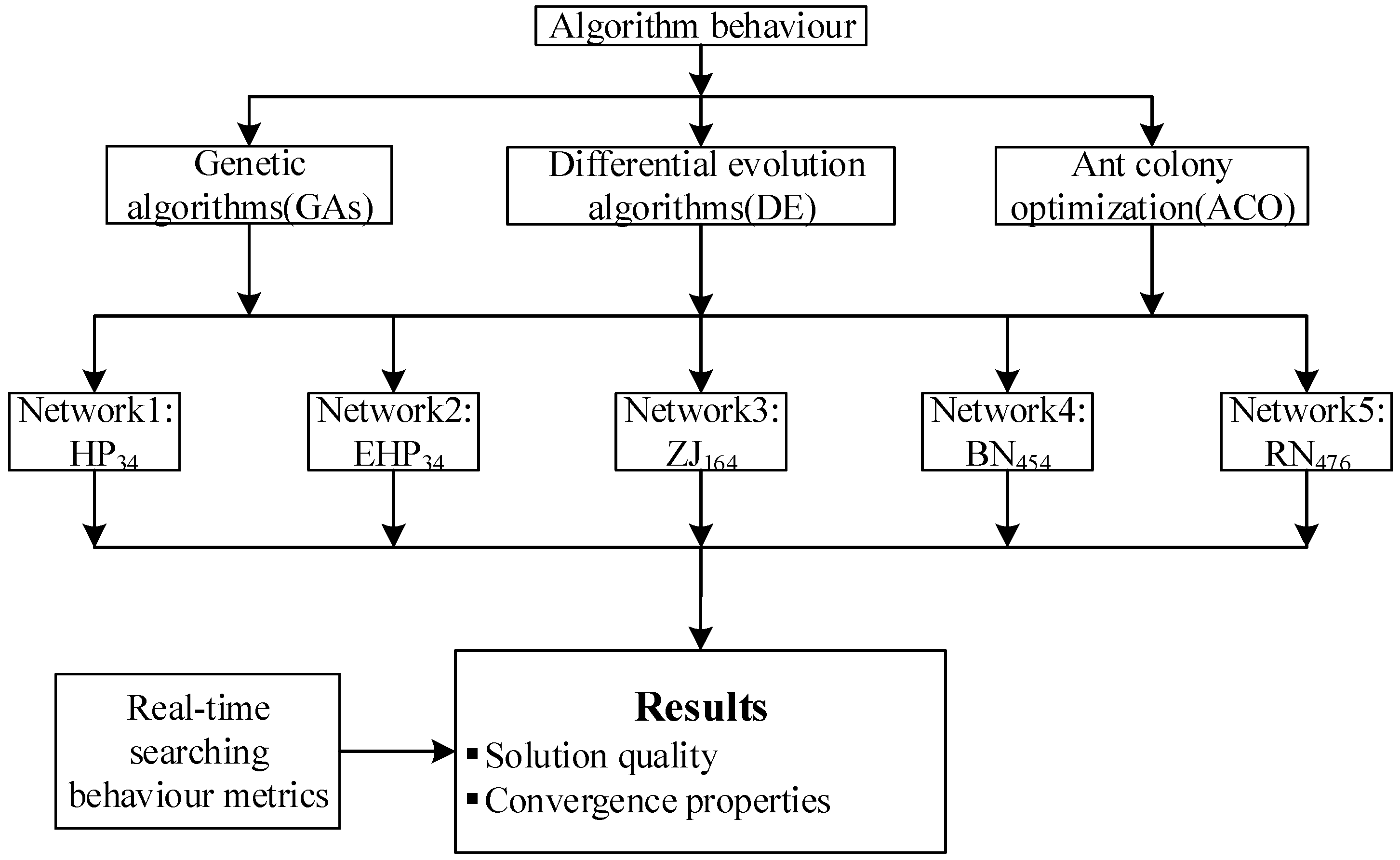
Figure 1 is the overall method of this study. As shown in this figure, three different types of EAs are considered. To better reflect the performance of the algorithms applied to different types of WDS design problems, the three EAs are applied to five different types of WDS design problems, with the number of decision variables ranging from 34 to 476. In order to better understand the search characteristics of three EAs, the search behaviour of the runtime algorithm is analysed. The information of each component of Figure 1 is described in details in the following subsections.

2.1. Evolutionary Algorithms and Their Parameterization

The GAs used in this study involve an integer coding, two-point crossover, bitwise mutation and constraint tournament selection following the previous papers [17,33,34], where the crossover, mutation and the selection operators are used to drive the searching towards optimal solutions. The standard differential evolution (DE) algorithm includes three operators, which are mutation, crossover and selection operators. The DE differs significantly from a GA in the mutation process whereby the mutant solution is generated by adding the weighted difference between several random population members to another random member [12]. The ACO is a population-based meta-heuristic analogically derived from the foraging behaviour of a colony of ants [22]. The $A{S}_{rank}$ algorithm is used in this paper as it has shown a better performance than other ACO variant [29].

The parameterization strategy of each EA is taken from previous studies [28,30,34,35] and the resultant parameters are outlined in

Table 1. Details of the parameterization strategies of the EAs applied to the five case studies. Parameters are as follows: where $N$ is the population size, $P_c$ and $CR$ are the crossover probabilities for the GA and DE respectively, $P_m$ and $F$ are their mutation probabilities; $\alpha$ = pheromone weighting factor; $\beta$ = visibility weighting factor; $\rho$ = pheromone decay factor; Q = pheromone update coefficient; N = number of ants; $\sigma$ = number of elitist ants; Maximum number of allowed generations for each algorithm is 10,000.

The Algorithm Name	Parameters of Each Algorithm	Parameter Values for Five Different Case Studies
		Hanoi (HP)	Extend Hanoi (EHP)	ZJ	Balerma (BN)	Rural Network (RN)
ACO	$N$	100	100	500	500	500
	$Q$	$1.1\times {10}^7$	$1.1\times {10}^7$	$5.3\times {10}^7$	$2.2\times {10}^7$	$5.3\times {10}^8$
	$\alpha$	1	1	1	1	1
	$\beta$	0.98	0.98	0.98	0.98	0.98
	$\sigma$	5	5	5	5	5
DE	$N$	100	100	500	1000	1000
	$F$	0.5	0.5	0.3	0.3	0.3
	$C_R$	0.5	0.5	0.5	0.5	0.5
GA	$N$	100	100	500	1000	1000
	$P_c$	0.9	0.9	0.9	0.9	0.9
	$P_m$	0.02	0.02	0.06	0.02	0.02

. It is noted that the searching behaviour of each EA may be affected by the parameterization of the controlling operators. The searching behaviour results presented in this study are conditioned on the default parameters that have been well calibrated for the three EAs in previous studies and, hence, these results are meaningful.

2.2. Case Studies

Within the optimization design of WDS, the decision variables are usually the diameters of the pipes in the system, and hence the number of decision variables equals to the number of pipes involved in the WDS [12]. The constraint conditions are often the minimum water supply pressure as well as the corresponding hydraulic equations that the system must meet [29].

For a given WDS optimization design problem with n pipes $D={\left[d_1,d_2,\cdots ,d_n\right]}^T$, the objective is to determine the least-cost solution $D^{*}$ while ensuring the solution meet design constraints, where:

$$D^{*}=argmin{\displaystyle \sum }_{i=1}^n{C}_i(d_i),$$

(1)

subject to:

$$P(D^{*})\ge P_{min},$$

(2)

$$d_i\in \left\{A\right\},$$

(3)

where $C_i$ = the cost function of the optimization design problem, which is related to decision variable $d_i$. It is noted that the cost considered in this study consists of the pipe material cost and the construction cost. $d_i$ = pipe diameter of pipe I = 1, 2, …, n; $P(D^{*})$ = the nodal pressure vector for solution $D^{*}$; $P_{min}$ = the vector of minimum pressure head that each node needs to meet; $\left\{A\right\}$ = a set of available pipe diameters for optimization design. In this study, EPANET 2.0 (Water Supply and Water Resources Division of the U.S. Environmental Protection Agency’s National Risk Management Research Laboratory, Cincinnati, Ohio, U.S.) is used as a hydraulic solver to calculate network pressure in this study.

As shown in Table 1 and Figure 1, five case studies of varying sizes and complexities are considered in this paper where the subscript indicates the number of decision variables for each case study in Figure 1.

Table 2. Details of the five case studies.

Case Study	No. of Decision Variables	No. of Diameter Options	Size of Total Search Space	Pressure Head Constraint	Reference
Hanoi (HP)	34	6	$2.86\times {10}^{26}$	$\ge 30\mathrm{m}$	[8]
Extend Hanoi (EHP)	34	10	$1\times {10}^{34}$	$\ge 30\mathrm{m}$	[34]
ZJ	164	14	$9.23\times {10}^{187}$	$\ge 22\mathrm{m}$	[36]
Balerma (BN)	454	10	$1\times {10}^{454}$	$\ge 20\mathrm{m}$	[17]
Rural network (RN)	476	15	$6.58\times {10}^{559}$	$\ge 0\mathrm{m}$	[37]

shows all details of the five case studies, including the number of decision variables (number of pipes), the pipe options, the size of the corresponding search space as well as the pressure head constraint. More details about the pipe network (such as the layout of the pipe network, the length of the corresponding pipe section, etc.) can be found in the literature given in Table 2.

3. Searching Measure Metrics

Five real-time search behaviour metrics are used to describe the real-time search behaviour of the three EAs applied, including the search quality metrics and the convergence metrics, with details shown below.

3.1. Search Quality Measure Metrics

For the optimization problem with a single objective, the quality of the solution refers to the closeness of the identified solutions to the known optimal solution during the searching process. $f_{best}(G)$ is the most intuitive quality measure metric [29], where it represents the best solution found at each iteration [38,39], that is, the optimal solution at each generation (G) of the solution set f(x):

$$f_{best}(G)=\min \left\{f(X)\right\},$$

(4)

This metric can be used to describe the change in algorithm performance as the number of iterations increases. Another quality measure metric is $f_{avg}(G)$, which represents the overall quality of the searching population. It can be expressed as:

$$f_{avg}(G)=\frac{1}{N}\sum f(X),$$

(5)

where $X\in \left\{X_{1,G},\dots ,X_{N,G}\right\}$ = the set of N solution vectors at generation G = 1, 2, …, $G_{max}$.

The percentage of feasible solutions ($PF\%$) in the population at generation G can also be used as a quality metric. The feasible solution means that a solution meets the hydraulic constraints, i.e., the solution satisfies Equation (2). It can be expressed as:

$$\begin{array}{c}PF\%(G)=\frac{1}{N}{\displaystyle {\displaystyle \sum }_{i=1}^N}I(P(X_{i,G}),P_{min}),\end{array}$$

(6)

where:

$$\begin{array}{c}I=(P(X_{i,G}),P_{min})=\{\begin{array}{cc}1& P(X_{i,G})\ge P_{min}\\ 0& otherwise\end{array},\end{array}$$

(7)

where $P(X_{i,G})$ is the pressure head at each node of the WDS for the $X_{i,G}$ solution, which is calculated using a hydraulic solver.

3.2. Convergence Measure Metrics

Zecchin et al. and Zheng identified the degree of convergence and population diversity in the decision space by using the average of the pairwise total hamming distances in the decision space [12,29]. It can be described as:

$$\begin{array}{c}{D}_{mean}(G)=\frac{2}{N(N-1)}{\displaystyle {\displaystyle \sum }_{i=1}^{N-1}}{\displaystyle {\displaystyle \sum }_{k=i+1}^N}H({\overrightarrow{X}}_{i,G},{\overrightarrow{X}}_{k,G}),\end{array}$$

(8)

where $N(N-1)$ = the total number of pairs of the candidate solutions; $H({\overrightarrow{X}}_{i,G},{\overrightarrow{X}}_{k,G})$ is a topological distance function used to calculate the hamming distance between the two solutions of ${\overrightarrow{X}}_{i,G}$ and ${\overrightarrow{X}}_{k,G}$ at generation G, and it can be expressed as:

$$H({\overrightarrow{X}}_{i,G},{\overrightarrow{X}}_{k,G})=\langle \left[\begin{array}{c}{x}_{j,i,G}\\ ⋮\\ x_{D,i,G}\end{array}\right],\left[\begin{array}{c}{x}_{j,k,G}\\ ⋮\\ x_{D,k,G}\end{array}\right]\rangle ={\displaystyle \sum }_{j=1}^n{I}_H(x_{j,i,G},x_{j,k,G})$$

(9)

$I_H$ can be expressed as:

$$\begin{array}{c}{I}_H=(x_{j,i,G},x_{j,k,G})=\{\begin{array}{cc}0& x_{j,i,G}=x_{j,k,G}\\ 1& otherwise\end{array},\end{array}$$

(10)

In addition to $D_{mean}(G)$, Zheng proposed another metric, which is the percentage of the best solution to the population in each generation [12]. It can be mathematically expressed

$$\begin{array}{c}PB\%(G)=\frac{1}{N}{\displaystyle {\displaystyle \sum }_{i=1}^N}{I}_H({\overrightarrow{X}}_{i,G},{\overrightarrow{X}}_G^{*})\times 100\%,\end{array}$$

(11)

where ${\overrightarrow{X}}_G^{*}$ is the best solution in the decision space identified by the EA at generation G. If ${\overrightarrow{X}}_{i,G}$ = ${\overrightarrow{X}}_G^{*}$, $I_H$ = 1; otherwise, $I_H$ = 0. This metric is used to measure the selection pressure during the algorithm’s search process, and the selection pressure can directly affect the quality of the best solution and the time required for the search. When the value of $PB\%$ is slowly increasing or fluctuating slightly, the algorithm selection pressure is small, and the search space can be widely searched, this meaning that better solutions can be identified with a high likelihood. In contrast, if the value of $PB\%$ increases with a larger rate as the number of iterations increases, the selection pressure of the algorithm is large and it is easy to fall into a local optimal solution.

4. Case Study Results and Discussion

4.1. Search Quality Results

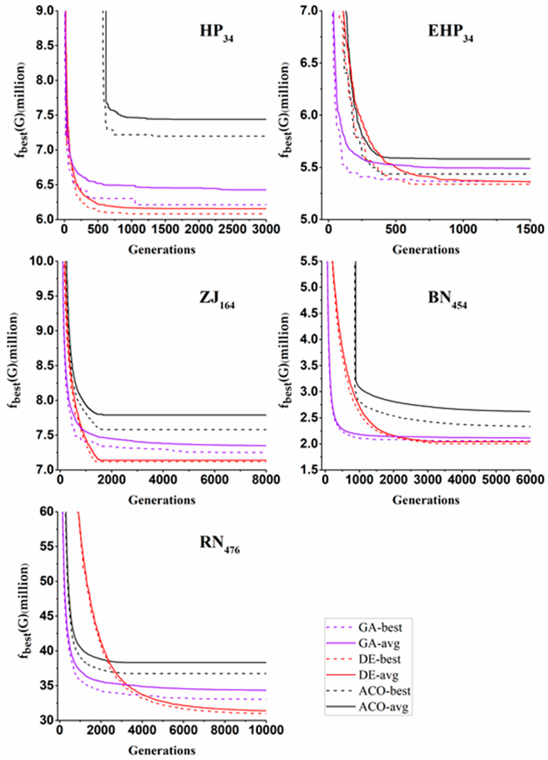
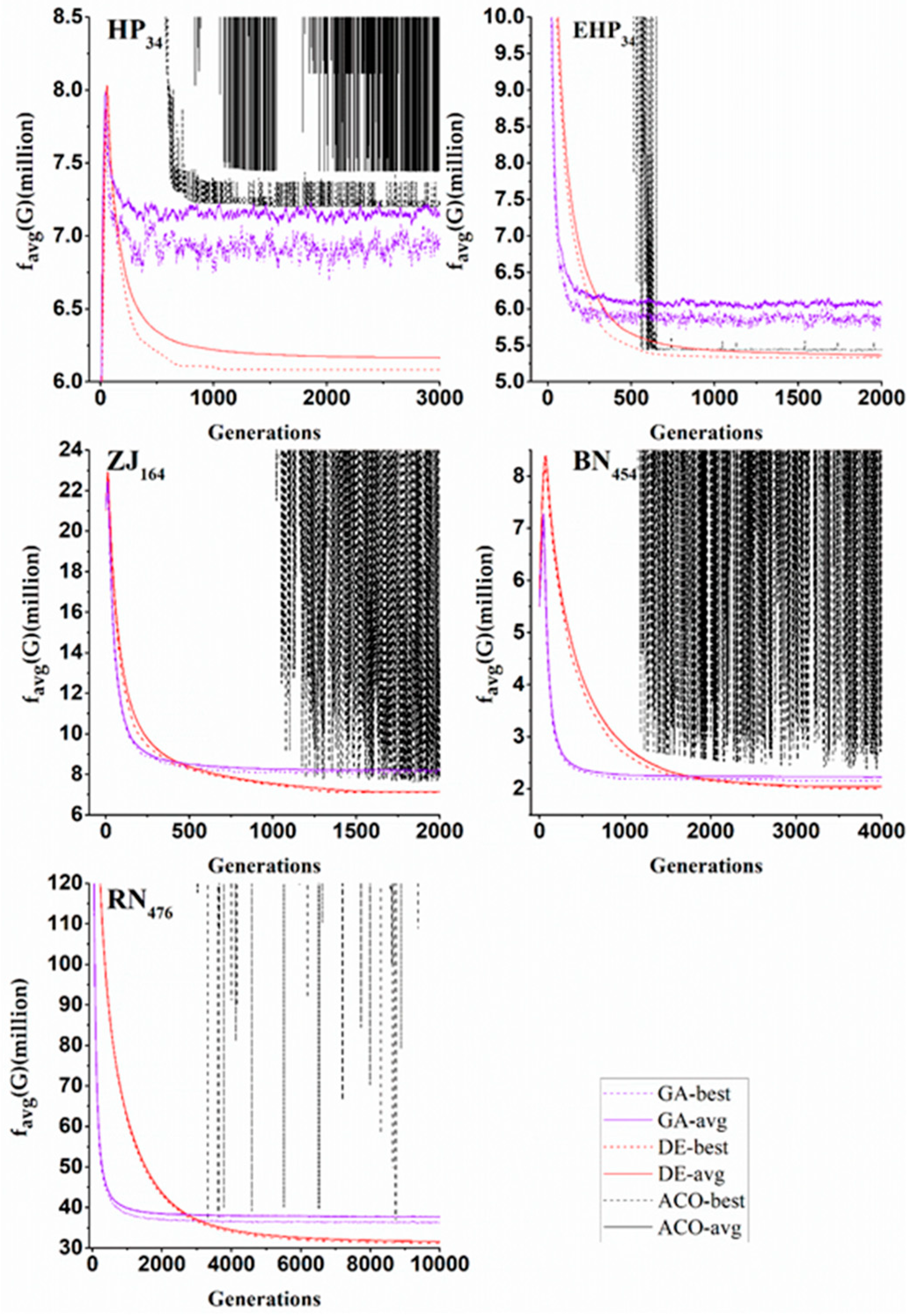
Figure 2, Figure 3 and Figure 4 show the results of search quality metrics when the GA, DE and ACO are applied to five case studies. It is noted that for the relatively small case studies (HP and EHP), 50 runs are performed with different random number seeds, but 10 runs are performed for the ZJ, BN and RN case studies. The averaged performances across different runs as well as the best run are presented to enable the analysis. From the change curve of the metrics with the increase of the number of iterations (G), a pattern applicable to all the three EAs can be summarized: the solution is rapidly improved during the early searching stage, followed by gradual enhancements with a slow rate. Interestingly, during the early stage in the search, compared to the other two algorithms, GA can find better solutions for the five case studies as shown in Figure 2 and Figure 3. However, as the number of iterations increases (during the middle-later searching stages), the solutions found by DE gradually outperform GA and ACO. Generally, the ACO performs the worst for all the case studies.

For $Z{J}_{164}$, $B{N}_{454}$, $R{N}_{476}$ case studies, the performance differences of the three EAs in identifying optimal solutions are obvious. For $R{N}_{476}$ and $B{N}_{454}$ case studies, the solutions found by the DE algorithm are significantly better than the other two EAs during the later searching stages, which is especially the case for the $R{N}_{476}$ case study. More specifically, the solution quality of the GA and ACO was rapidly improved before 2000 generations, followed by a very slow further improvement later on. However, the DE algorithm can consistently improve its searching quality throughout the searching process. This implies that the DE is more robust in exploring the searching space relative to the GA and ACO.

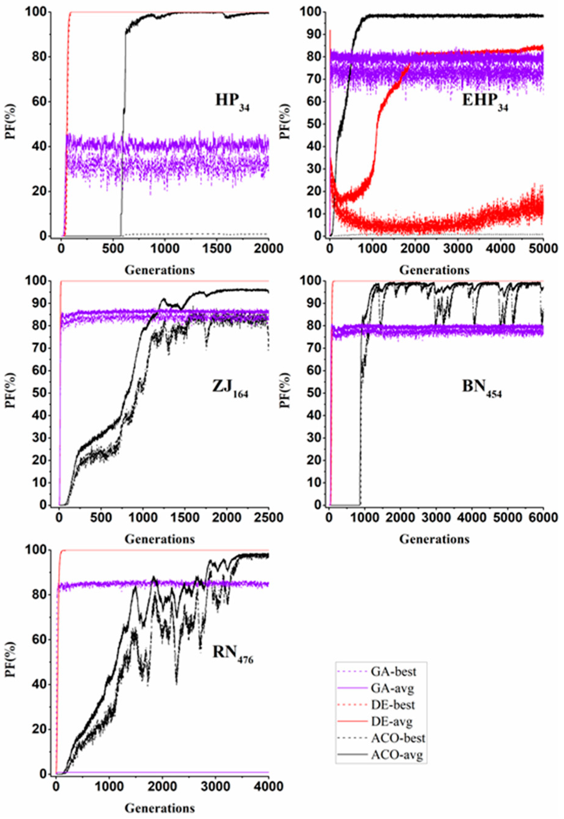
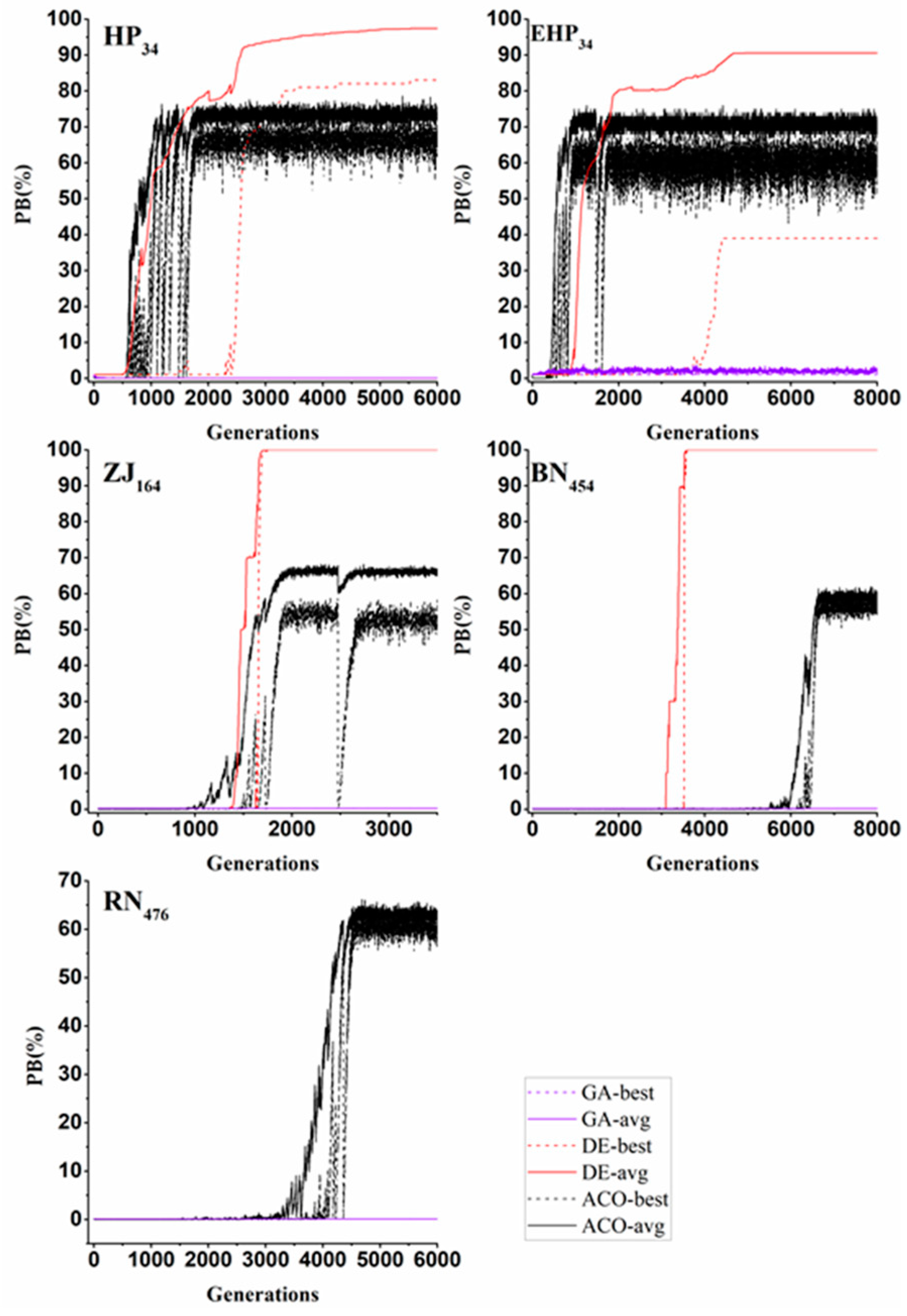
The ability of the three EAs in identifying feasible solutions is outlined in Figure 4. It is seen from this figure, the DE overall possesses the best ability in locating the feasible solutions. This is supported by the observations that the DE can drive its population towards the feasible regions of the searching space with a fast rate for the four case studies, but not for the EHP problem. This demonstrates that the searching behaviours of the EAs can be also affected by the fitness landscape properties of the case studies. For the GAs, it is found that they can identify the feasible regions quickly, but they always maintain a small proportion of the searching efforts in the infeasible regions. This can be related to the mutation strategy used by the GA. The ACO identify feasible solutions with a slower rate compared with the DE, but it mainly focuses on the feasible region during the moderate–later searching stages.

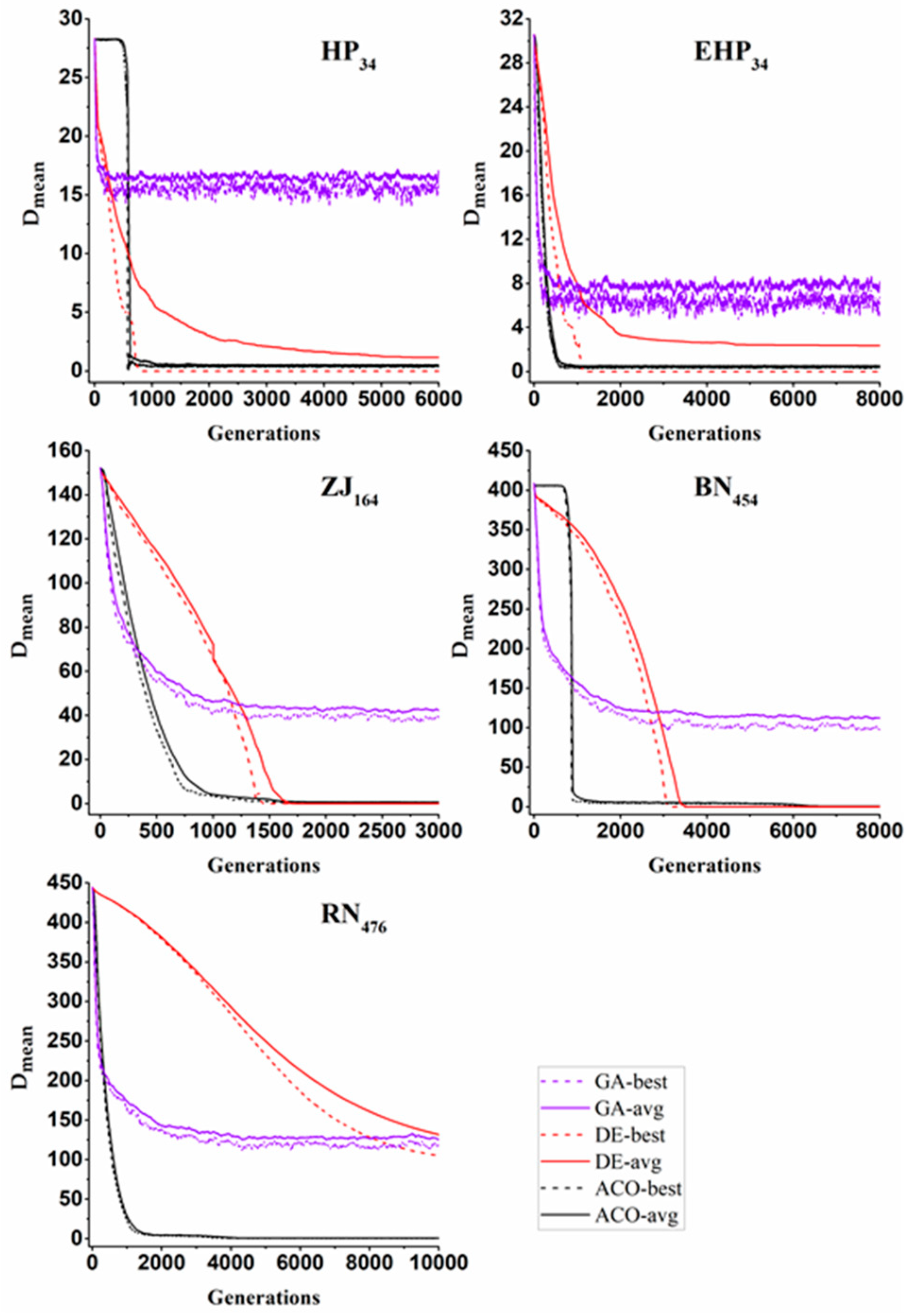
4.2. Convergence Measure Results

Figure 5 and Figure 6 show the results of convergence metrics when GA, DE and ACO were applied to the five case studies. As shown in these figures, at the initial stage of the search, the $D_{mean}(G)$ values of the three EAs decreased at a faster rate, corresponding to the rapid improvement of the quality of the solution in Figure 2. This shows that the search is effective during the fast convergence phase of the algorithm. As shown in Figure 5, the convergence rate of the three EAs is slowing down as the scale and complexity of the case study increase. In terms of convergence speed, GA consistently has the fastest convergence speed at the initial searching stage for all case studies, but ACO converges quickly during the middle-later stages. DE exhibits the mild convergence rate in the decision space as shown in Figure 5. In addition, it can be observed that as the scale and complexity of the case study increase, the differences between the convergence speeds of the three algorithms becomes more apparent. It is worth noting that in the late search period, the three EAs exhibit different search behaviours. In the later stage of the search, the $D_{mean}(G)$ of the GA keeps a high value and fluctuates slightly. This means that the GA’s searching still maintains a high population diversity in the later stage. Combining with results in Figure 4, it can be deduced that GA still maintains a certain amount of search in the infeasible solution regions in the later stage of the search.

As shown in Figure 5, during the later stage of the search, the DE focuses on the searching in the surrounding regions of the identified best solution. This is followed by that the $D_{mean}(G)$ converges to 0 as well as that the $PB\%(G)$ = 100 in Figure 6, implying that all individuals in the population locate the identical best solution. However, this is not the case for the RN case study due to its greatly increased complexity and, hence, the DE is unable to entirely converge for the given computational budgets.

The convergence speed of ACO is least affected by the increasing complexity of case studies. In the later stage of the search, the $D_{mean}(G)$ value of ACO stabilized at a small value, and the population maintained a certain diversity. It is worth mentioning that in the earliest stages of search, ACO maintains a large $D_{mean}(G)$, which means that during this period, ACO conducts broad search on the search space. Combining the higher $PF\%(G)$ values in Figure 4 and the fluctuating $f_{avg}(G)$ values in Figure 2, it can be deduced that at this stage, the search of ACO is concentrated at the boundary between the feasible and infeasible solution regions [29].

As shown in Figure 6, the GA’s $PB\%(G)$ value remains at a very small value and fluctuates in the entire search process until the maximum number of iterations. After a sufficient search, DE forces the entire population to find the best solution. This means that in the subsequent search phase, DE is under the greatest selection pressure and GA is the smallest. This is related to their selection strategy and mutation strategy. It is noted that the ACO consistently shows the worst performance in terms of the averaged metric values across multiple runs. This indicates that the ACO’s poor performance is more likely to be caused by its underlying searching mechanisms, instead of the randomness of the initial solutions.

4.3. Solution Comparisons

Table 3. Solution statistics of the three algorithms, where the percentage indicates the difference between the best solutions found by the three algorithms in this study and the current best known solutions in literature.

Case Studies	Current Best Known Solution	GA			DE			ACO
		Best Solution	Worst Solution	Average Cost	Best Solution	Worst Solution	Average Cost	Best Solution	Worst Solution	Average Cost
Hanoi (HP) ($M)	6.081 [17]	6.174 (1.5%)	6.560	6.395	6.081 (0%)	6.329	6.155	7.198 (18.4%)	7.761	7.440
Extend Hanoi (EHP) ($M)	5.346 [34]	5.357 (0.2%)	5.616	5.460	5.338 (−0.2%)	5.364	5.341	5.432 (1.6%)	5.718	5.582
ZJ ($M)	7.082 [36]	7.248 (2.3%)	7.509	7.345	7.125 (0.6%)	7.176	7.140	7.579 (7.0%)	8.0362	7.787
Balerma (BN) (€M)	1.923 [36]	2.045 (6.3%)	2.152	2.103	2.002 (4.1%)	2.075	2.040	2.332 (21.3%)	2.846	2.618
Rural Network (RN) ($M)	31.220 [37]	33.010 (5.7%)	35.821	34.332	30.989 (−0.7%)	31.776	31.396	36.737 (17.7%)	39.963	38.332

outlines the solution statistics of the three algorithms, where the current best known solution for each case study is also presented. It is seen from this table that the DE is able to find the current best known solutions for the HP and EHP, and even better solutions for the RN case study. For the ZJ and BN case studies, the solutions found by the DE are very close to their current best known optimal solutions. The ACO algorithm performs the worst in terms of the end-of-run solutions, and the ACO shows slightly worse performance than the DE algorithm.

5. Conclusions

This paper makes the first attempt to compare the real-time searching behaviour of three widely used EAs within the WDS design domain with the aid of five metrics regarding searching quality and convergence properties. These are GAs, DE and ACO, and they are applied to five WDS design problems with increasing complexity. The results of the metrics have verified the applicability of real-time search behaviour metrics to different types of EAs. In addition, this study has proved that compared to traditional methods, run-time search behaviour metrics can deeply reveal the algorithm’s searching characteristics. The main findings and the implications based on this study are given below.

• The three EAs have exhibited significantly different searching behaviours in both the solution space and decision space. Such differences can be related to their underlying model structures and the searching mechanisms. This demonstrates that the proposed run-time metrics are effective in revealing the searching properties of the EAs.
• From the obtained real-time metric results, it can be concluded that the DE has an overall best ability to locate feasible solutions as well as high quality solutions for the WDS design problems. The ACO performed overall the worst in identifying the optimal solutions as observed in this study. This provides a guideline for the selection of the algorithms for WDS design optimization.
• If the computational budget is rather limited, the GA can identify better solutions than the DE as shown in this study. This suggests that the GA is promising for the case when the optimization solution needs to be identified in a short time such as real-time WDS operation and management.

References

- Maier, H.R.; Kapelan, Z.; Kasprzyk, J.; Kollat, J.; Matott, L.S.; Cunha, M.C.; Dandy, G.C.; Gibbs, M.S.; Keedwell, E.; Marchi, A.; et al. Evolutionary algorithms and other metaheuristics in water resources: Current status, research challenges and future directions. Environ. Model. Softw. 2014, 62, 271–299. [Google Scholar] [CrossRef] [Green Version]
- Nicklow, J.; Reed, P.; Savic, D.; Dessalegne, T.; Harrell, L.; Chan-Hilton, A.; Karamouz, M.; Minsker, B.; Ostfeld, A.; Singh, A.; et al. State of the art for genetic algorithms and beyond in water resources planning and management. J. Water Resour. Plan. Manag. 2010, 136, 412–432. [Google Scholar] [CrossRef]
- El-Ghandour, H.A.; Elbeltagi, E. Comparison of five evolutionary algorithms for optimization of water distribution networks. J. Comput. Civ. Eng. 2018, 32, 04017066. [Google Scholar] [CrossRef]
- Monsef, H.; Naghashzadegan, M.; Jamali, A.; Farmani, R. Comparison of evolutionary multi objective optimization algorithms in optimum design of water distribution network. Ain Shams Eng. J. 2019, 10, 103–111. [Google Scholar] [CrossRef]
- Mora-Melia, D.; Iglesias-Rey, P.L.; Martinez-Solano, F.J.; Ballesteros-Pérez, P. Efficiency of evolutionary algorithms in water network pipe sizing. Water Resour. Manag. 2015, 29, 4817–4831. [Google Scholar] [CrossRef]
- Guercio, R.; Xu, Z. Linearized optimization model for reliability-based design of water systems. J. Hydraul. Eng. 1997, 123, 1020–1026. [Google Scholar] [CrossRef]
- Sonak, V.V.; Bhave, P.R. Global optimum tree solution for single-source looped water distribution networks subjected to a single loading pattern. Water Resour. Res. 1993, 29, 2437–2443. [Google Scholar] [CrossRef]
- Fujiwara, O.; Khang, D.B. A two-phase decomposition method for optimal design of looped water distribution networks. Water Resour. Res. 1990, 26, 539–549. [Google Scholar] [CrossRef]
- Lansey, K.E.; Mays, L.W. Optimization model for water distribution system design. J. Hydraul. Eng. 1989, 115, 1401–1418. [Google Scholar] [CrossRef]
- Maier, H.R.; Kapelan, Z.; Kasprzyk, J.; Matott, L.S. Thematic issue on evolutionary algorithms in water resources. Environ. Model. Softw. 2015, 69, 222–225. [Google Scholar] [CrossRef] [Green Version]
- Ji, C.; Jiang, Z.; Sun, P.; Zhang, Y.; Wang, L. Research and application of multidimensional dynamic programming in cascade reservoirs based on multilayer nested structure. J. Water Resour. Plan. Manag. 2015, 141, 04014090. [Google Scholar] [CrossRef]
- Zheng, F. Comparing the real-time searching behavior of four differential-evolution variants applied to water-distribution-network design optimization. J. Water Resour. Plan. Manag. 2015, 141. [Google Scholar] [CrossRef]
- Bi, W.; Maier, H.R.; Dandy, G.C. Impact of starting position and searching mechanism on the evolutionary algorithm convergence rate. J. Water Resour. Plan. Manag. 2016, 142, 04016026. [Google Scholar] [CrossRef]
- Holland, J.H. Adaptation in Natural and Artificial Systems; MIT Press: Cambridge, MA, USA, 1992. [Google Scholar]
- Zheng, F.; Zecchin, A.C.; Simpson, A.R.; Lambert, M.F. Noncrossover dither creeping mutation-based genetic algorithm for pipe network optimization. J. Water Resour. Plan. Manag. 2014, 140, 553–557. [Google Scholar] [CrossRef] [Green Version]
- Zheng, F.; Simpson, A.R.; Zecchin, A.C. A decomposition and multistage optimization approach applied to the optimization of water distribution systems with multiple supply sources. Water Resour. Res. 2013, 49, 380–399. [Google Scholar] [CrossRef] [Green Version]
- Reca, J.; Martínez, J. Genetic algorithms for the design of looped irrigation water distribution networks. Water Resour. Res. 2006, 42, W05416. [Google Scholar] [CrossRef]
- Mambretti, S. Optimization of the pumping station of the milano water supply network with genetic algorithms. In Energy and Sustainability III; WIT Press: Southampton, UK, 2011; pp. 185–194. [Google Scholar]
- Li, M.; Liu, S.; Zhang, L.; Wang, H.; Meng, F.; Bai, L. Non-dominated sorting genetic algorithms-iibased on multi-objective optimization model in the water distribution system. Procedia Eng. 2012, 37, 309–313. [Google Scholar] [CrossRef] [Green Version]
- Suribabu, C.R. Differential evolution algorithm for optimal design of water distribution networks. J. Hydroinform. 2010, 12, 66–82. [Google Scholar] [CrossRef]
- Zheng, F.; Zecchin, A. An efficient decomposition and dual-stage multi-objective optimization method for water distribution systems with multiple supply sources. Environ. Model. Softw. 2014, 55, 143–155. [Google Scholar] [CrossRef]
- Maier, H.R.; Simpson, A.R.; Zecchin, A.C.; Foong, W.K.; Phang, K.Y.; Seah, H.Y.; Tan, C.L. Ant colony optimization for design of water distribution systems. J. Water Resour. Plan. Manag. 2003, 129, 200–209. [Google Scholar] [CrossRef] [Green Version]
- Szemis, J.M.; Maier, H.R.; Dandy, G.C. A framework for using ant colony optimization to schedule environmental flow management alternatives for rivers, wetlands, and floodplains. Water Resour. Res. 2012, 48, W08502. [Google Scholar] [CrossRef] [Green Version]
- Szemis, J.M.; Maier, H.R.; Dandy, G.C. An adaptive ant colony optimization framework for scheduling environmental flow management alternatives under varied environmental water availability conditions. Water Resour. Res. 2014, 50, 7606–7625. [Google Scholar] [CrossRef] [Green Version]
- Nguyen, D.C.H.; Maier, H.R.; Dandy, G.C.; Ascough, J.C. Framework for computationally efficient optimal crop and water allocation using ant colony optimization. Environ. Model. Softw. 2016, 76, 37–53. [Google Scholar] [CrossRef]
- Nguyen, D.C.H.; Ascough, J.C.; Maier, H.R.; Dandy, G.C.; Andales, A.A. Optimization of irrigation scheduling using ant colony algorithms and an advanced cropping system model. Environ. Model. Softw. 2017, 97, 32–45. [Google Scholar] [CrossRef]
- Foong, W.K.; Maier, H.R.; Simpson, A.R. Power plant maintenance scheduling using ant colony optimization: An improved formulation. Eng. Optim. 2008, 40, 309–329. [Google Scholar] [CrossRef] [Green Version]
- Zecchin, A.C.; Simpson, A.R.; Maier, H.R.; Nixon, J.B. Parametric study for an ant algorithm applied to water distribution system optimization. IEEE Trans. Evol. Comput. 2005, 9, 175–191. [Google Scholar] [CrossRef] [Green Version]
- Zecchin, A.C.; Simpson, A.R.; Maier, H.R.; Marchi, A.; Nixon, J.B. Improved understanding of the searching behavior of ant colony optimization algorithms applied to the water distribution design problem. Water Resour. Res. 2012, 48, W09505. [Google Scholar] [CrossRef] [Green Version]
- Zheng, F.; Zecchin, A.C.; Newman, J.P.; Maier, H.R.; Dandy, G.C. An adaptive convergence-trajectory controlled ant colony optimization algorithm with application to water distribution system design problems. IEEE Trans. Evol. Comput. 2017, 21, 773–791. [Google Scholar] [CrossRef]
- Yazdi, J.; Choi, Y.H.; Kim, J.H. Non-dominated sorting harmony search differential evolution (ns-hs-de): A hybrid algorithm for multi-objective design of water distribution networks. Water 2017, 9, 587. [Google Scholar] [CrossRef] [Green Version]
- Zheng, F.; Zecchin, A.C.; Maier, H.R.; Simpson, A.R. Comparison of the searching behavior of nsga-ii, samode, and borg moeas applied to water distribution system design problems. J. Water Resour. Plan. Manag. 2016, 142, 04016017. [Google Scholar] [CrossRef]
- Simpson, A.R.; Dandy, G.C.; Murphy, L.J. Genetic algorithms compared to other techniques for pipe optimization. J. Water Resour. Plan. Manag. 1994, 120, 423–443. [Google Scholar] [CrossRef] [Green Version]
- Bi, W.; Dandy, G.C.; Maier, H.R. Improved genetic algorithm optimization of water distribution system design by incorporating domain knowledge. Environ. Model. Softw. 2015, 69, 370–381. [Google Scholar] [CrossRef]
- Zheng, F.; Zecchin, A.C.; Simpson, A.R. Investigating the run-time searching behavior of the differential evolution algorithm applied to water distribution system optimization. Environ. Model. Softw. 2015, 69, 292–307. [Google Scholar] [CrossRef] [Green Version]
- Zheng, F.; Simpson, A.R.; Zecchin, A.C. A combined nlp-differential evolution algorithm approach for the optimization of looped water distribution systems. Water Resour. Res. 2011, 47, W08531. [Google Scholar] [CrossRef] [Green Version]
- Marchi, A.; Dandy, G.; Wilkins, A.; Rohrlach, H. Methodology for comparing evolutionary algorithms for optimization of water distribution systems. J. Water Resour. Plan. Manag. 2014, 140, 22–31. [Google Scholar] [CrossRef]
- Hansen, N.; Müller, S.D.; Koumoutsakos, P. Reducing the time complexity of the derandomized evolution strategy with covariance matrix adaptation (cma-es). Evol. Comput. 2003, 11, 1–18. [Google Scholar] [CrossRef] [PubMed]
- Deb, K.; Beyer, H.G. Self-adaptive genetic algorithms with simulated binary crossover. Evol. Comput. 2001, 9, 197–221. [Google Scholar] [CrossRef]
Figure 1.
The overall methodology of the proposed method.
Figure 2.
Solution quality metric of the three different types of EAs applied to the five case studies.
Figure 3.
Figure 4.
Figure 5.
Figure 6.