Estimating Current and Future Rainfall Erosivity in Greece Using Regional Climate Models and Spatial Quantile Regression Forests


Department of Rural and Surveying Engineering, Aristotle University of Thessaloniki, 54124 Thessaloniki, Greece
*
Author to whom correspondence should be addressed.
Water 2020, 12(3), 687; https://doi.org/10.3390/w12030687
Submission received: 14 February 2020
/
Revised: 29 February 2020
/
Accepted: 1 March 2020
/
Published: 3 March 2020
(This article belongs to the Special Issue Rainfall Erosivity in Soil Erosion Processes)
Abstract
:A future variation of precipitation characteristics, due to climate change, will affect the ability of rainfall to precipitate soil loss. In this paper, the monthly and annual values of rainfall erosivity (R) in Greece are calculated, for the historical period 1971–2000, using precipitation records that suffer from a significant volume of missing values. In order to overcome the data limitations, an intermediate step is applied using the calculation of monthly erosivity density, which is more robust to the presence of missing values. Spatial Quantile Regression Forests, a data driven algorithm that imitates kriging without the need of strict statistical assumptions, was utilized and validated, in order to create maps of R and its uncertainty using error propagation. The monthly average precipitation for the historical period 1971–2000 estimated by five (5) Global Circulation Models-Regional Climatic Models were validated against observed values and the one with the best performance was used to estimate projected changes of R in Greece for the future time period 2011–2100 and two different greenhouse gases concentration scenarios. The main findings of this study are: (a) the mean annual R in Greece is 1039 MJ·mm/ha/h/y, with a range between 405.1 and 3160.2 MJ·mm/ha/h/y. The highest values are calculated at the mountain range of Pindos and the lowest at central Greece; (b) the monthly R maps adhere to the spatiotemporal characteristics of precipitation depth and intensities over the country; (c) the projected R values, as an average over Greece, follow the projected changes of precipitation of climatic models, but not in a spatially homogenous way.
1. Introduction
Rainfall erosivity concerns the ability of rainfall to precipitate soil loss [1], as it supplies energy to the mechanical processes of soil erosion. Decertification has been identified as one of the most serious issues facing Mediterranean European countries, including Greece [2], and a possible increase in future rainfall, due to climate change, will aggravate this process, as soil erosion increases at a greater rate [3]. Unanticipatedly, a decrease in future rainfall and a possible decrease of biomass production may also lead to higher erosion rates [4].
Higher erosion rates in conjunction with unsustainable land management and increasing human pressure can lead to soil degradation [5], and consequently a disrupted ecological balance, a decreasing agricultural production and income [6] and even the reduction of effectiveness of adaptation options [7]. Several issues may arise due to accelerated soil losses on achieving of the Sustainable Development Goals of the United Nations [8], as these goals are dependent on a healthy biophysical environment in which the soil is the base [9]. In order to predict these soil erosion future changes it is necessary to simulate changes in future rainfall erosivity, land uses and the application of policies on land management [10].
Universal Soil Loss Equation (USLE) [11], which is the most widely used soil erosion prediction model in the world [12], is an empirical equation that estimates the long-term, average, rate of soil loss involving the product of six factors. The USLE erosivity factor, R, is calculated using high frequency or break-point precipitation data with a duration of over 20 years [13,14], as a function of rainfall intensity and depth. In the second revised version of USLE, RUSLE2 [15], monthly Erosivity Density (ED) was introduced, as a measure of rainfall erosivity per unit rainfall, which requires shorter precipitation record lengths. ED is approximately a function of values only related to rainfall intensity and was used in RUSLE2 as an intermediate step, in conjunction with coarser, monthly, precipitation data, to compute R values in the USA.
Precipitation in Greece has been investigated in several studies over the past two decades [16,17,18,19,20,21,22,23]. In general, precipitation varies from its maximum values during winter to a minimum during summer. The highest precipitation values are observed on the mountain range of Pindos, and its expansion on Peloponnesus, and the lowest values of precipitation are recorded on the Cyclades Islands, at the center of the Aegean Sea. Due to the fact that most weather systems and prevailing winds are moving over the Ionian Sea perpendicularly to Pindos, a contrast exists between the wetter western parts of the country and the dryer eastern ones. During summer months convective activity over northern Greece produces higher precipitation amounts than over the drier southern parts.
Global Circulation Models (GCMs) are models that represent the atmosphere, land surface, ocean and sea ice and simulate their interactions in three dimensions, to make long-term predictions of climate [24]. Different scenarios about future concentrations of greenhouse gases (Representative Concentration Pathways, RCPs) are employed to describe a set of different climate futures that drive GCMs [25]. Due to the coarse grid scale of GCMs (over 80 to ~300 km), Regional Climate Models (RCMs) were developed to downscale them and provide information on a finer scale, more applicable to local scaled phenomena, impact studies and adaptation decisions. RCMs are dependent on GCMs, because GCMs provide the response of global circulation, greenhouse gases concentrations, etc. and RCMs refine them in a spatiotemporal sense, using features such as the topography, coastlines, land cover or mesoscale dynamics [26]. The climatic models from COordinated Regional Climate Downscaling EXperiment over Europe (EURO-CORDEX) [27], using high-resolution RCMs for the high greenhouse gases concentration scenario, RCP8.5, project a decrease of precipitation from 1971–2000 to 2071–2100 and for the medium concentration scenario, RCP4.5, project the same trend with a smaller magnitude [27,28]. Regarding rainfall intensity, in the form of heavy precipitation that exceeds the intensity at the 95th percentile of daily precipitation, the same models project diverging trends that are not statistically significant in most areas of Greece [27,28].
In our previous studies about ED in Greece [29,30] it was proven that, in general, ED values are robust to the presence of missing values in contrast to R, which is highly affected, and specifically in Greece: (a) the values of ED are not significantly correlated with the elevation, (b) ED annual timeseries are found to be stationary, in contrast to reported precipitation trends for the same time period and (c) ED can be considered as spatially autocorrelated, as three contiguous areas were identified using clustering analysis, that had distinct temporal patterns. A comparison of our studies with an earlier study about R in Greece by Panagos et al. [31] revealed that the previously reported R values were underestimated due to the presence of a significant volume of missing data in the precipitation records used in the calculations.
In the Mediterranean region, the annual R model MedREM was developed using annual precipitation depth, the longitude and annual daily maximum precipitation data [32]. A recent paper regarding the estimation of future R values in Europe for 2050 [10], used one GCM and a single RCP, applied Gaussian Process Regression using monthly variables obtained from the WorldClim dataset [33] and estimated an increase of R by 14.8% in Greece. A number of papers in Europe examined the potential increase of rainfall erosivity using temporal trends of high resolution precipitation data in Western Germany [34], Belgium [35] and in the Czech Republic [36]. Other studies in various parts of the world used GCMs in conjunction with empirical equations that predict R using annual precipitation [37,38], monthly [39,40] and daily rainfall indices [41,42]. A different approach estimated projected R changes, using a weather generator with spatial and temporal downscaled precipitation values coming from various GCMs [43].
Random Forests [44] is a data-driven algorithm in the area of supervised learning which tries to fit a model using a set of paired input variables and their associated output response and can be used in classification and regression problems. Quantile Regression Forests (QRF) [45], is an extension of RF that is able to compute prediction intervals of the output response in regression problems. RF has been used for spatial prediction in various domains [46,47,48,49,50] and recently, Hengl et al. [51] presented RF for a spatial predictions framework, that can make equally accurate predictions as kriging, without the need of statistical assumptions.
The aim of this work is to calculate the current and estimate the future changes of R values in Greece. The latest methodologies developed and presented with RUSLE2 are used, taking into account the presence of missing values in precipitation records. The first objective of the analysis is to create monthly precipitation and ED maps, as intermediate datasets, and to estimate the uncertainty of their predictions and their errors using cross-validation. Consequently, the current R values in Greece are computed from the interpolated surfaces and error propagation is used to estimate approximately their uncertainty. Finally, downscaled precipitation from GCMs-RCMs is validated and used, along with ED, to estimate the potential changes of R in Greece for the years 2040, 2070 and 2100 using two future greenhouse gases concentration trajectories/pathways (i.e., RCPs). This type of analysis is a novel approach and it has not been presented, until now, in the international literature.
2. Materials and Methods
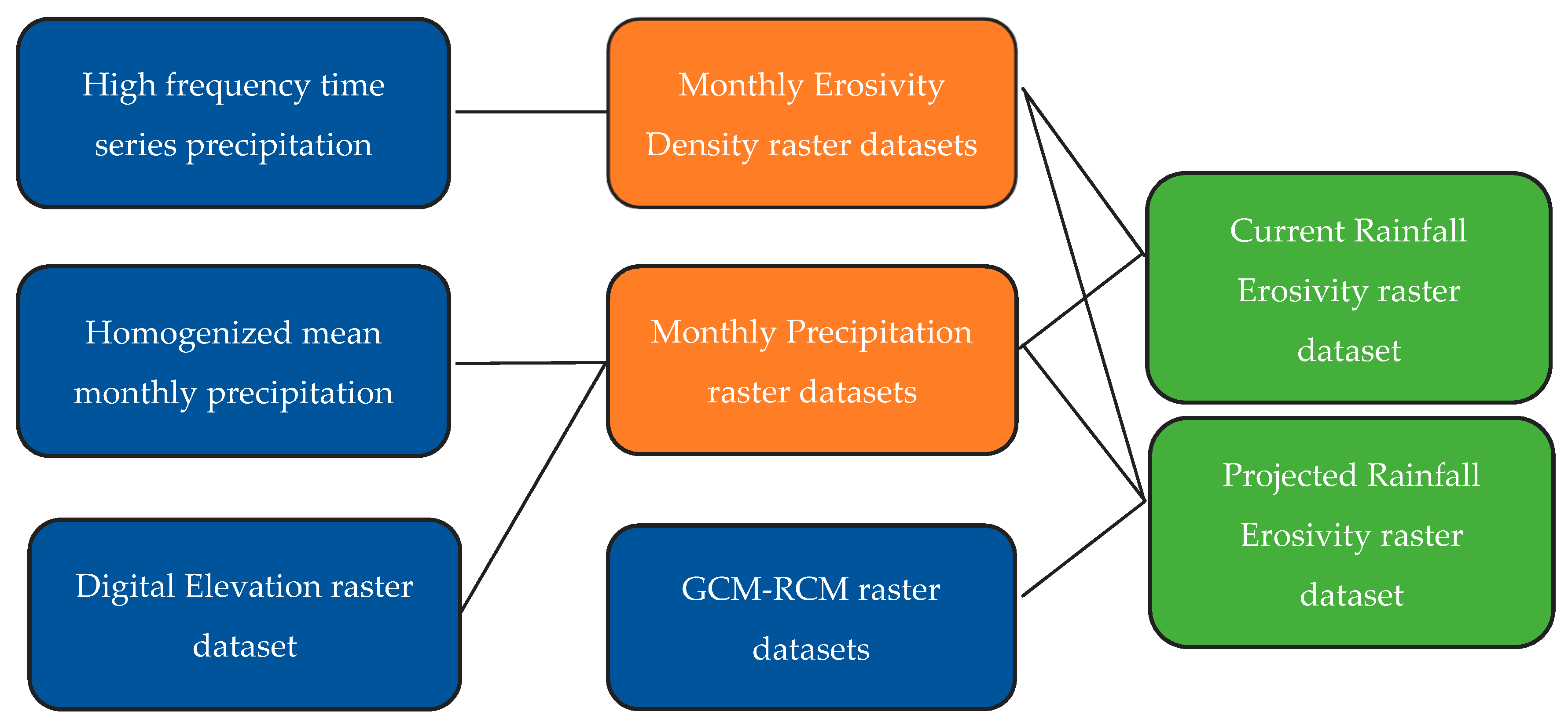
The methodology that was applied in the study, is presented in the flowchart of Figure 1, where data flows from the left to the right. Blue symbolizes the data that were used as input (pointwise and raster), orange the intermediate raster datasets that were created and green the final results, also in raster format, that were computed using different sets of input and intermediate datasets.
2.1. Data Acquisition and Processing
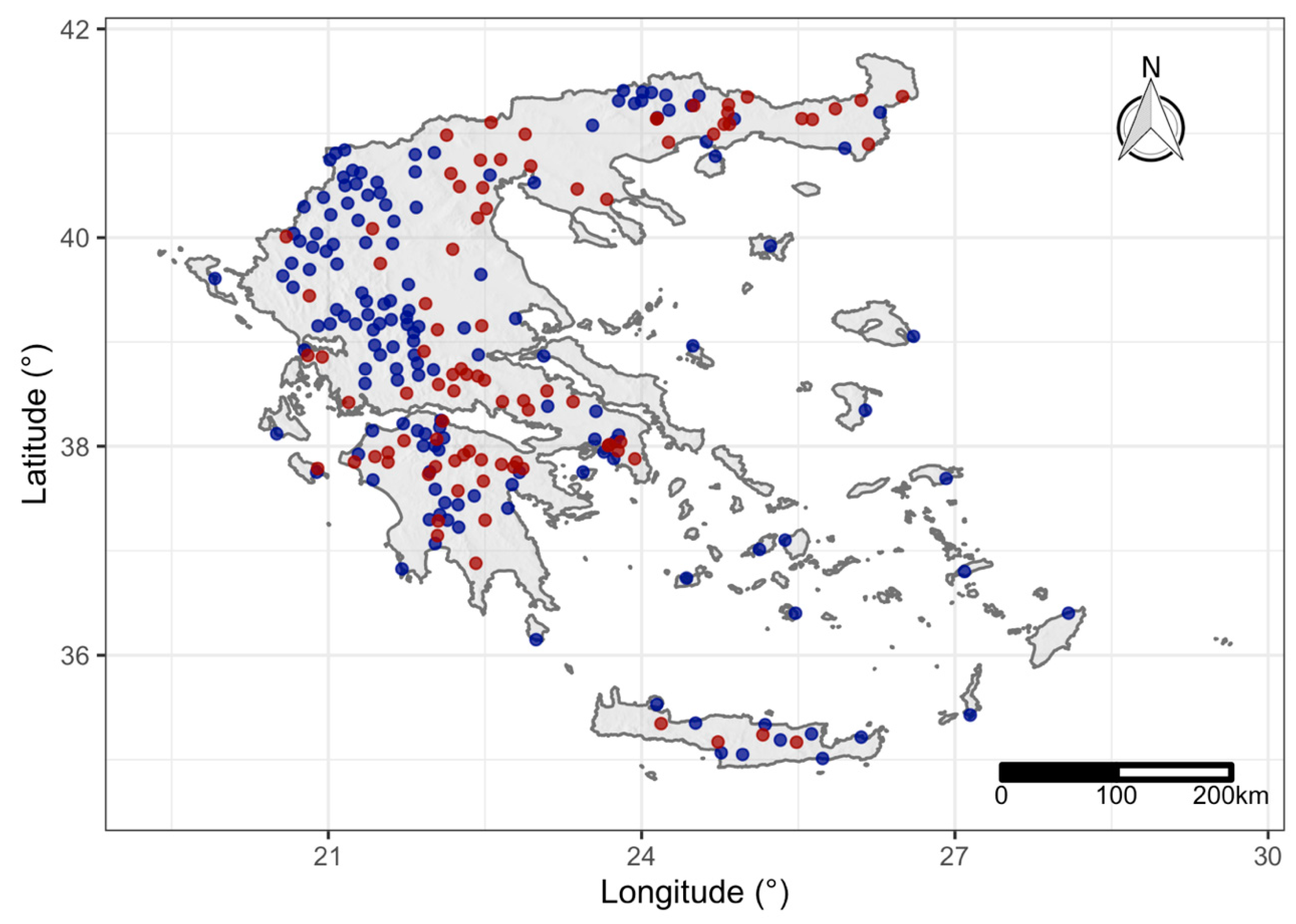
Point precipitation data from 237 meteorological stations across Greece (Figure 2), was used in the analysis. The data consisted of:
- Pluviograph data for 87 meteorological stations that were taken from the Greek National Bank of Hydrological and Meteorological Information (NBHM) [52]. The time series comprised a total of 2273 years of 30-min-records and 394 years of five-min-records for the time period from 1953 to 1997, with a mean length of 30 years per station. The timeseries coverage was 62.8% on average.
- Mean monthly precipitation data for 150 meteorological stations that were taken from the Hellenic National Meteorological Service (HNMS) [53]. These are homogenized data and available for the time period from 1971 to 2000. These data were used to overcome the limitations of precipitation data from NBHM.
- Five different monthly GCM-RCM raster datasets were downloaded for a number of experiments and time periods (Table 1). These data were computed in the framework of the EURO-CORDEX [27,54], had a horizontal resolution 0.11° × 0.11° and were remapped using bilinear interpolation to a 30″ × 30″ resolution grid using the Climate Data Operator (CDO) software [55].
The GCM-RCM monthly precipitation timeseries data were:
- Historical, for the time period from 1971 to 2000 (like the ones coming from HNMS) as they were driven by the boundary conditions provided by the GCMs.
- Future, for the forcing scenarios RCP4.5 (where greenhouse gases emissions peak around 2040 and then decline) and RCP8.5 (where greenhouse gases emissions continue to rise throughout the 21st century), using the control ensemble of the CORDEX climate projection experiments. The dataset period was from 2011 to 2100.
Digital elevation raster data were downloaded from the NASA Shuttle Radar Topography Mission (SRTM) [56], and aggregated to the same 30″ × 30″ resolution grid as the one used in the GCM-RCMs datasets.
2.2. Monthly Erosivity Density Calculation
The erosivity of a single erosive rainfall event, (MJ·mm/ha/h), given the product of the kinetic energy of rainfall and its maximum 30 min intensity, was computed using the pluviograph records from NBHM [15]:
where is the kinetic energy per unit of rainfall (MJ/ha/mm), the rainfall depth (mm) for the time interval of the hyetograph, which has been divided into time sub-intervals and is the maximum rainfall intensity for a 30 min duration during that rainfall.
The quantity was calculated for each time sub-interval, , applying the kinetic energy equation that was used in RUSLE2 [57], which was recently evaluated in Italy, a nearby country to Greece, and had the best performance among alternative literature expressions [58]:
where is the rainfall intensity (mm/h).
An individual rainfall event was extracted from the continuous pluviograph data, if its cumulative depth for a duration of 6 h at a certain location was less than 1.27 mm. A rainfall event was considered to be erosive if it had a cumulative rainfall depth greater than 12.7 mm. Only the screened events with a return period of less than 50 years were used in the calculations.
On the grounds that the use of coarser fixed time intervals to a finer one can lead to an underestimation of the value of erosivity [59,60], monthly conversion factors were computed using the five-min-time-step timeseries:
where is the number of storms at month m, is the erosivity of a storm using the five min time step and the erosivity of the same storm when the timeseries was aggregated using a 30 min time step. These conversion factors were applied to the values of erosivity that were estimated from 30-min pluviograph data.
After the computation of values, the average monthly rainfall erosivity density (MJ/ha/h) per station was calculated:
where is the number of storms during the month , the erosivity of storm , the monthly precipitation height and the number of years.
2.3. Spatial Quantile Regression Forests
Random Forests (RF) [44] is one of the most successful methods used in Machine Learning [61], among other reasons because of: (a) its robustness to outliers [62] and overfitting [63], (b) its ability to perform feature selection [64] and (c) the fact that its default parameters, as implemented in software, give satisfactory results [61,65]. Examples of RF open source software are the R’s language packages randomForest [66] and its faster alternative, ranger [67].
In summary, RF consists of a number of decision trees [68]. For each tree, a random set of the dataset is created via bootstrapping [69] and in each node of the tree a random set of n input variables from the p variables of the dataset is considered to pick the best split [70]. The prediction of the output response in regression problems is the mean value of the estimations of these random decision trees. The estimate of the out-of-sample error is computed using the out-of-bag error [71], without the need of cross-validation.
Quantile Regression Forests (QRF) is an extension of RF that provides information about the full conditional distribution of the output response and not only about its mean [45], as is the case in plain RF. In this way, it is possible to provide prediction intervals and measures of uncertainty.
The use of QRF as a framework for the modeling of spatial variables was introduced by Hengl et al. [51], where the distances among observation locations are used as variables in QRF in order to incorporate geographical proximity effects. In this way, using these buffer distances, spatial QRF imitate kriging’s spatial correlation. Spatial QRF (spQRF) produces comparable results, in terms of accuracy, compared to the state-of-the-art kriging methods, with the advantage of no prior assumptions about the distribution or stationarity of the response variable [51].
In this work, spQRF were used for the spatial prediction of monthly precipitation and ED:
- The 12 monthly ED models (one model for each month of the year) were trained using as input variables the buffer distances for each one of the 87 stations of NBHM in a chained procedure [72]. In that procedure, at the first run, only the distances are used as input variables and at the nth both distances and the monthly results from the previous step, with the exception of the month that is the output response. This procedure stops when the out-of-sample error estimated by RFs in the form of out-of-the-bag error ceases to decrease.
- The 12 monthly precipitation models were trained using as input variables the buffer distances for each one of the 150 stations of HNMS and elevation data from the SRTM.
As a measure of the out-of-sample error, the average Root Mean Squared Error (RMSE), the coefficient of determination R2 and Lin’s Concordance Correlation Coefficient (CCC) were computed using 10-fold cross validation:
where is the total number of cross-validation locations, is the predicted value of at a cross-validation location (i.e., the coordinates longitude and latitude of location ), , , , are the means and variances of and , respectively, and is the covariance of and .
describes the ratio of variance that is explained by a model and may be negative, among other reasons, if an inappropriate model is used [73]. CCC combines measures of both precision and accuracy and examines how far deviate from the line of perfect concordance (the line of 45 degrees on a square scatterplot) and ranges from 0 to ±1 [74,75].
The uncertainty of the predictions from the models, in the form of prediction error standard deviation, was computed using a dense level of all the quantiles per 1% of the output response and for every location [51]:
where is the pth percentile of the distribution of the response variable at location and the mean value of for all the percentiles.
The quantity z-score, which quantifies the error of prediction errors, was calculated at cross validation locations [76]:
where , ideally, should have a mean equal to zero and variance equal to one. On the contrary:
- If variance(z) >> 1, the model underestimates the actual prediction uncertainty.
- If variance(z) << 1, the model overestimates the actual prediction uncertainty.
2.4. Regional Climate Models Historical Precipitation Validation
In order to validate and select one of the GCMs-RCMs for the projected erosivity calculations, at first, a multi-layer raster dataset was computed for each of the five models with the overall 30-year-mean-monthly precipitation values, using the historical time period from 1971 to 2000. Then, using the monthly precipitation spQRF models to create raster datasets with the same 30″ × 30″ resolution grid, RMSE, CCC and R2 errors metrics were computed, setting in Equations (5)–(7) as the values estimated by GCMs-RCMs and as the values calculated by the spQRF models.
2.5. Current and Projected Erosivity Calculation
The estimation of current and future monthly erosivity was made under the assumption of future temporal stationarity of ED values, due to the fact that ED is related to seasonal rainfall intensity [15] and EURO-CORDEX GCMs-RCPs models does not project statistically significant trends in most areas of Greece [27]. Temporal stationarity of ED values already has been documented in Greece for the historical period [30].
The current monthly erosivity was calculated as the product of predictions of the trained spQRF models of monthly and precipitation for each month m:
The prediction error standard deviation of monthly was calculated using error propagation [77]:
In order for Equation (11) to hold true, and were considered as the true values on locations and that were independent of each other. More specifically, these values were considered, to a good approximation, as not correlated on the basis of the following remarks:
- came from monthly average data and from random proportions of pluviograph data due to missing values.
- In general, precipitation depth, alone, is a poor indicator of erosivity [78].
The annual rainfall erosivity and its error standard deviation were calculated, respectively:
The projected values of monthly erosivity were computed using the ratio of the future 30-years-mean to the historical 30-years-average-monthly precipitation values that came from a GCM-RCM:
where f is the future year in which long term average monthly values refer to and:
The projected annual erosivity was estimated with:
And the ratio of future to current values:
With Equations (14)–(17), the projected annual erosivity values were calculated preserving the relative projected changes of precipitation without the direct use of simulated values coming from a GCM-RCM and the need to apply a bias-correction method. However, the need to use a statistical downscaling technique to apply bias correction to the GCM + RCM output will be tested.
3. Results and Discussion
3.1. Precipitation and ED Pointwise Values
The monthly conversion factors that were computed specifically for Greece using the five-min-time-step timeseries have a mean value 1.22, close to the one calculated for Europe [59], but had different seasonality with their maximum values in the period from May to October and minimum during March (Table 2).
The first four central moments (mean, standard deviation, skew and kurtosis) and other statistical properties were used to describe the calculated monthly values of ED (87 stations from NBHM, Table 3) and the average monthly precipitation (150 stations from HNMS, Table 4).
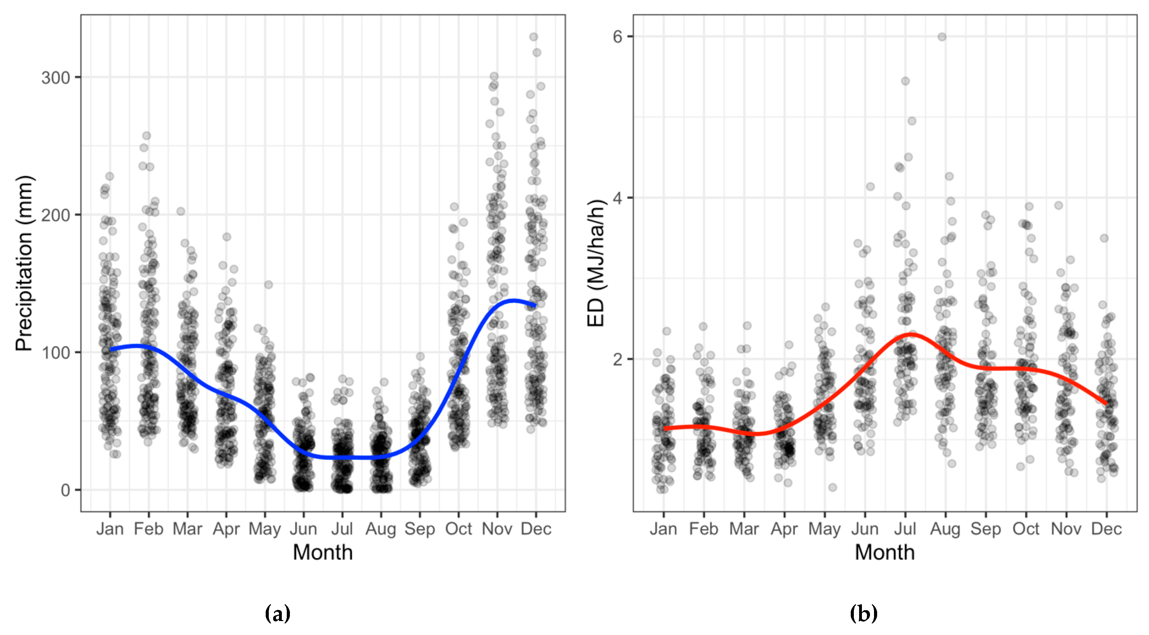
Monthly precipitation and ED had different monthly temporal patterns (Figure 3). The temporal pattern of precipitation is typical for a Mediterranean area with the minimum precipitation occurring during summer and the maximum precipitation observed in November and December (Figure 3a). This temporal pattern of monthly precipitation is typical for Greece [80]. The second had an almost bimodal shape with its two peaks at July and October. The values of ED were slightly different from the ones already reported in our previous work [30], due to the application of the seasonal monthly conversion factors to a constant one.
3.2. Spatial Models of Precipitation and ED
The training and cross validation of the spatial models was made using the implementation of QRF in the ranger [67] package of language R [82]. The number of trees was set to 1000 and the fine-tuning of the parameters of the model was made using the tuneRanger [83] package.
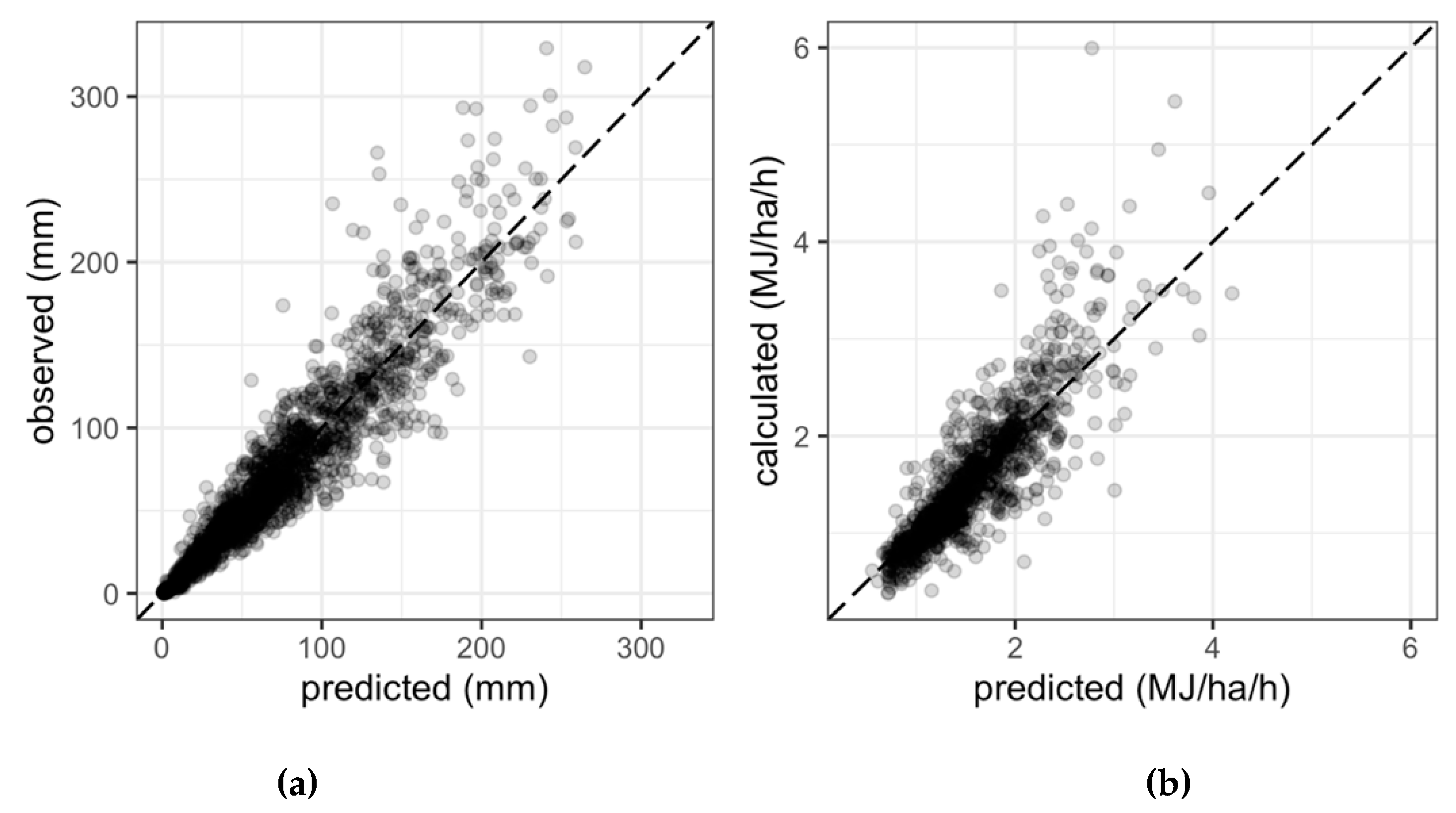
The cross validation error metrics of the models for monthly precipitation were satisfactory (Table 5), especially comparing them to recent precipitation models for Greece that showed weak correlation during the spring season [17] or equally good estimations [23]. As most months had a z-score variance smaller than one, these monthly models overestimated the actual prediction uncertainty (i.e., the error of prediction the error from the models in cross-validation locations).
The same cross validation error metrics of the models for monthly ED did not show equally good performance (Table 6), as most months had moderate results with the exception of summer months that had poor results. These poor results were coming from the scarcity of the stations used and the predictions of high ED values that the models underestimated them (Figure 4b), affecting especially RMSE and R2 metrics that are sensitive to outliers. Given the values of z-score’s variance, in general, also, most of the monthly ED models overestimated the actual prediction uncertainty.
3.3. Rainfall Erosivity and Its Uncertenty
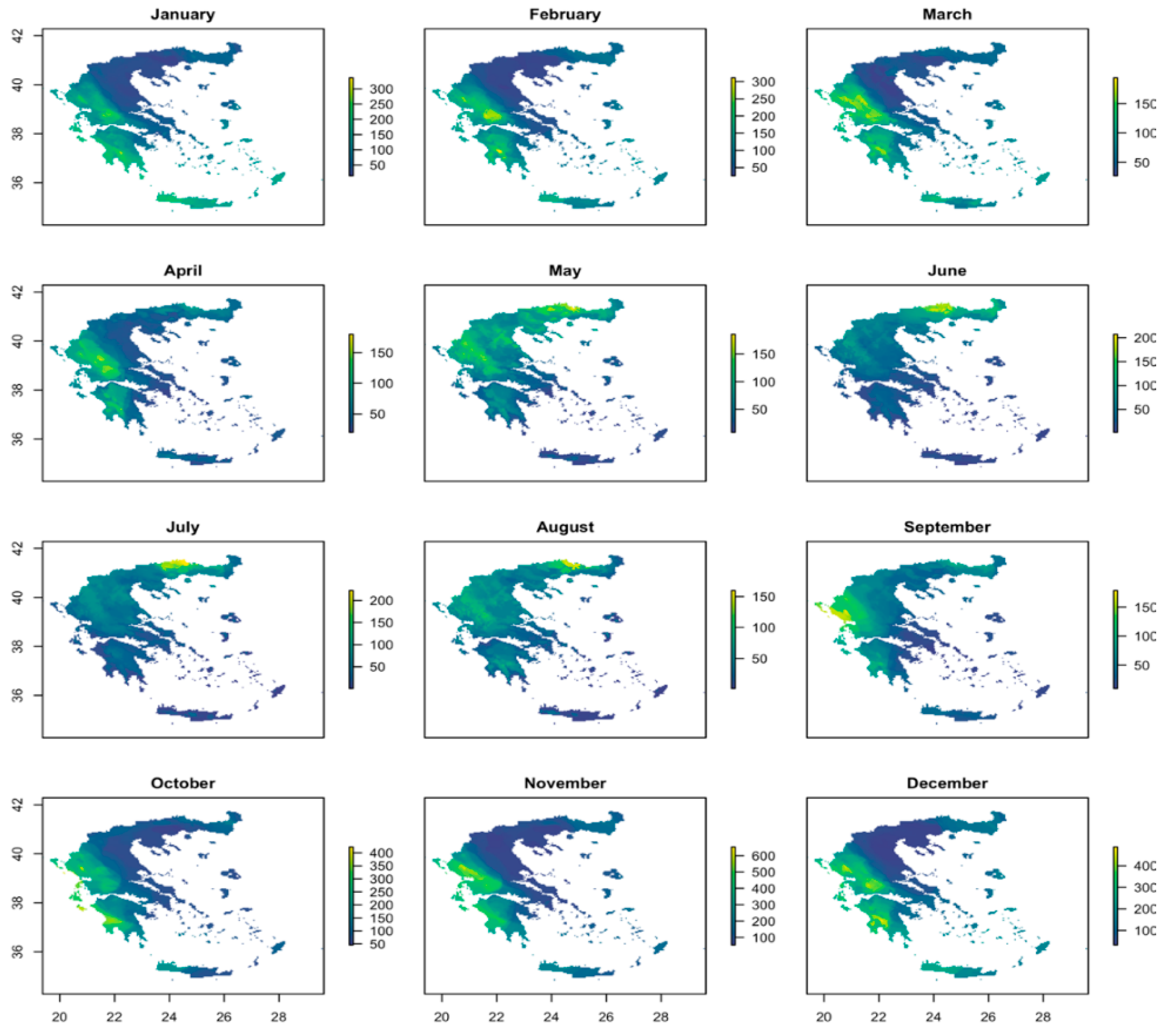
The produced maps (Figure 5 and Figure 6) illustrate the spatiotemporal distribution of R in Greece. The eastern, dryer part of the country has lower values than the wetter western part for the period during autumn and winter. During summer the convective activity over norther Greece produces higher R values than southern Greece, with the largest values occurring in the area of Thrace. The monthly temporal patterns illustrated in Figure 5, are compatible to the three areas that were identified in our previous study [30].
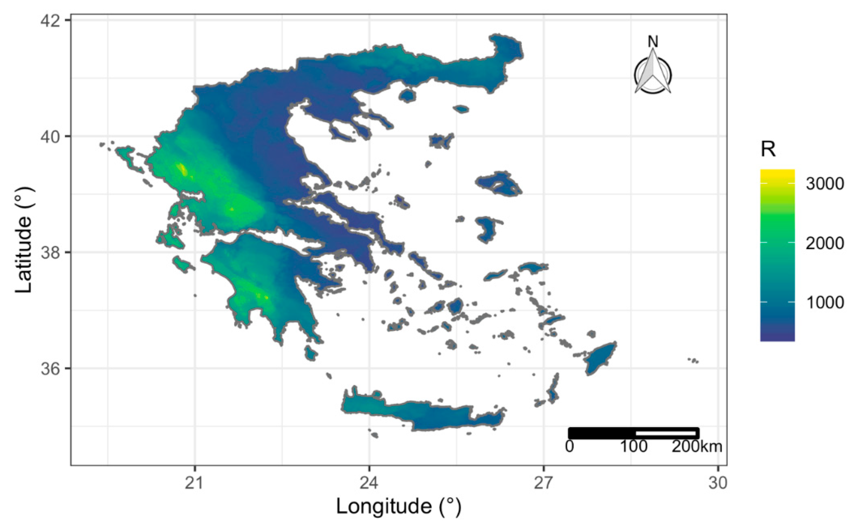
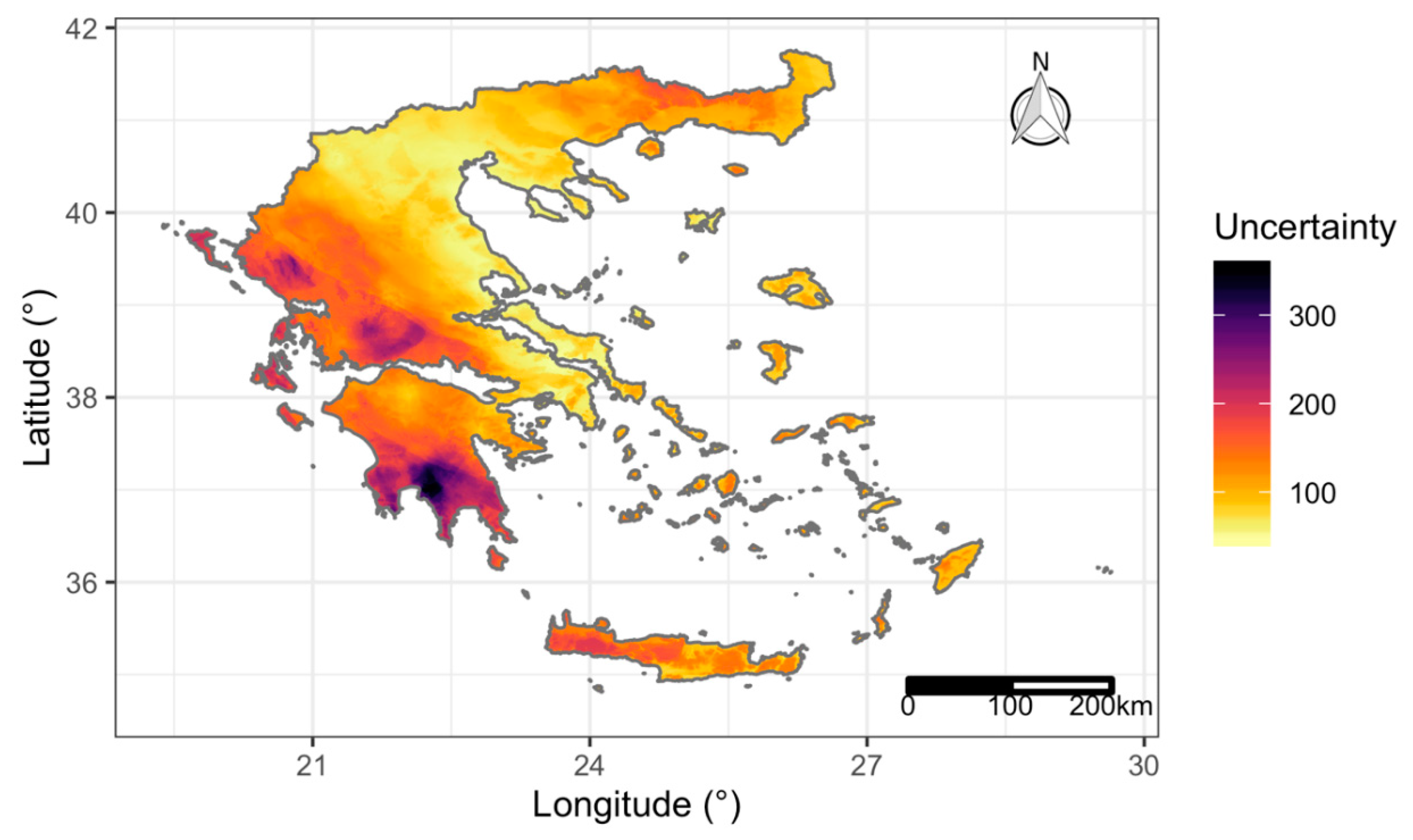
The lowest annual values of R were computed at the central mainland area of Greece (west and central Macedonia, Thessaly and Attica). The uncertainty map of annual R (Figure 7) follows the variation of the predicted annual erosivity and the scarcity of stations. The mean annual R (Table 7, Figure 6) has a value of 1039.0 MJ·mm/ha/h/y, with a range between 405.1 and 3160.2 MJ·mm/ha/h/y. The annual mean prediction error standard deviation is 116.9 MJ·mm/ha/h/y and its range is from 46.7 to 353.4 MJ·mm/ha/h/y (Table 7, Figure 7). The ratio of the mean annual error to the mean annual R is 11.25%, a value that was probably overestimated, given the cross-validation results of z-scores (Table 5 and Table 6). These errors are not considered very high, bearing in mind the spatially sparse data and the data-sets limitations. Although these errors may affect the reliability of the assessment of the potential impacts of climate change, their effect is rather small when compared with the large uncertainties in GCMs projections in monthly and daily precipitation and rainfall intensity [84].
The largest monthly mean R value are observed in November with 182.5 MJ·mm/ha/h/y and in December with 151.5 MJ·mm/ha/h/y and the lowest ones during summer months which have values about 44 MJ·mm/ha/h/y. The computed R values, due to the fact that R is linearly underestimated as the missing values ratio increases [30], were larger than the values reported by Panagos et al. [31] (i.e., the mean annual R was underestimated by 28.8%, the mean minimum by 381% and the maximum by 12%). On the contrary, the range of R values in this study is smaller (405.1–3160.2 MJ·mm/ha/h/y) than the respective values reported in [31] (was 84.2–2825 MJ·mm/ha/h/y).
In the above cited, older, study [31], the spatial distribution and annual values of R were affected by the used interpolated precipitation dataset. As a result, the highest values were calculated at the northwest corner of Greece. However, in this study, the maximum observed precipitation from HNMS’s stations were recorded at the mountain range of Pindos, which is, also, the area with the maximum annual R values in our study, indicating that the two variables are consistent.
3.4. Projected Rainfall Erosivity Changes
In order to cope with the uncertainties in climatic models, five (5) GCMs-RCMs were evaluated in terms of RMSE, R2 and CCC using the monthly precipitation maps that were created in this study. The EC-EARTH–KNMI-RACMO22E GCM-RCM (Table 8) gave the best results for each one of months and for all the error metrics. Given its performance, this GCM-RCM seemed to represent better monthly precipitation in Greece, for the historical time period and consequently used to estimate futures changes for the RCP forcing scenarios RCP4.5 and RCP8.5 and the years 2040, 2070 and 2100. However, the large errors presented in Table 8 indicate that statistical downscaling techniques have to be applied to the outputs of GCMs-RCMs for bias correction and reduction of errors.
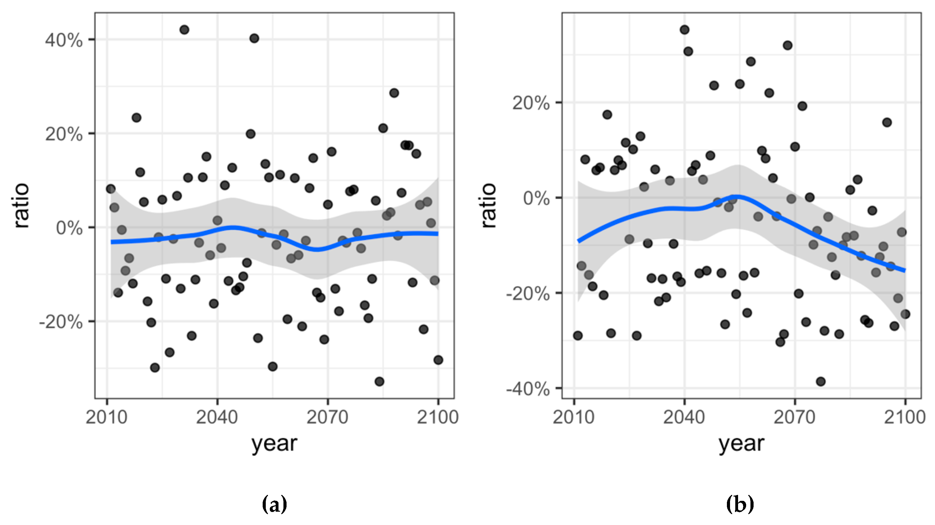
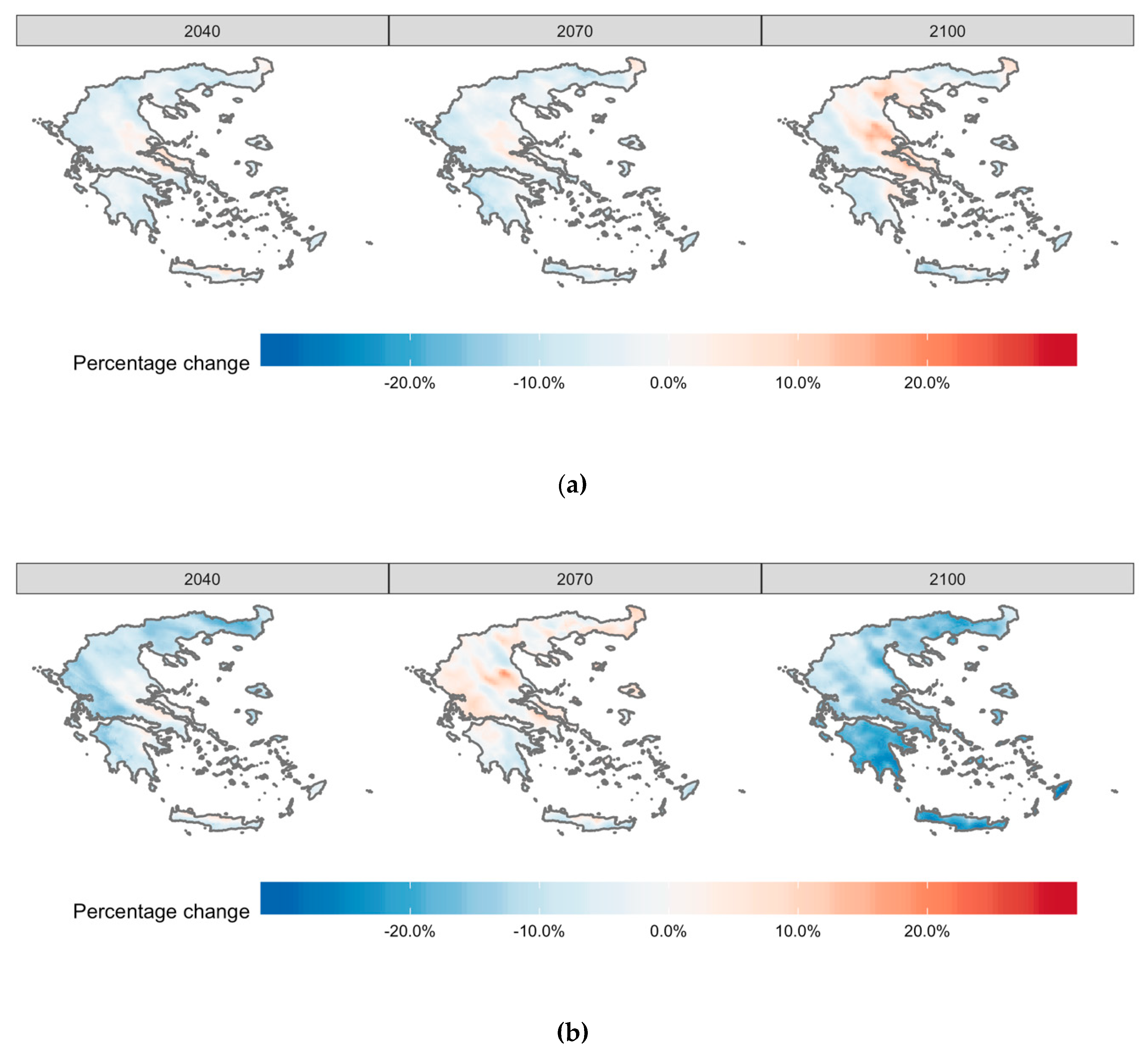
Using the RCP4.5 scenario, the ratio of the mean projected R to current values were −3.7%, −4.3% and −0.7% for 2040, 2070 and 2100, respectively. The same values for the RCP8.5, scenario were −9.0%, +0.01% and −14.6%. Annual R followed the annual ratio of projected to 30-years-mean historical precipitation, which fluctuated around zero for RCP4.5 (Figure 8a) and had a negative trend for the years 2040–2100 for RCP4.5.
Despite the decrease of the projected R values, using RCP4.5, R, spatially, has a tendency to increase at the central parts of Macedonia and Thessaly that have the highest agricultural productivity in the country and the northern Thrace (Figure 9a). For RCP8.5 (Figure 9b) projected erosivity increases on 2070, having a hotspot at Thessaly and then decreases, following the precipitation trend (Figure 8b). In the previously reported study concerning Europe, that did not use information about rainfall intensities in the applied model, the projected change of R values for Greece on 2050 was +14.8% using the GCM HadGEM2 and RCP4.5 [10].
The results of projected changes of R in both RCP scenarios are coherent to the precipitation trends that are reported by EURO-CORDEX, in which precipitation decreases by a larger magnitude in RCP8.5 than RCP4.5, from 1971–2000 to 2071–2100 [27]. This change in precipitation dominates in projected R’s calculations and is depicted in Figure 9b for the year 2100.
4. Conclusions
The estimation of mean annual and monthly R values over Greece using precipitation records that suffered from a significant volume of missing values was the main result of this paper, utilizing as an intermediate step the creation of monthly precipitation and ED QRF models. The models of monthly precipitation had better performance than the ones of monthly ED in terms of prediction accuracy, mostly due to the scarcity of stations with calculated ED values. Validating the error of uncertainty reported from the models on cross validation locations, showed that the models, on average, overestimate the actual prediction error (i.e., the error of error predictions). More specifically, the findings of the present study can be summarized as follows:
- The mean annual R in Greece is 1039 MJ·mm/ha/h/y, with a range between 405.1 and 3160.2 MJ·mm/ha/h/y, during the historical period 1971–2000. The highest values are calculated at the mountain range of Pindos and the lowest at central Greece’s mainland.
- The calculated monthly mean R values follow the already documented spatiotemporal characteristics of precipitation depth and intensity over the country.
- The climatic model EC-EARTH-KNMI-RACMO22E from the Royal Netherlands Meteorological Institute better reproduces the monthly precipitation for the historical period 1971–2000 in Greece than the other four GCMs-RCMs used and tested in this study.
- The projected mean annual erosivity, R, as an average over Greece, follows, in general, the projected changes of precipitation from the selected GCM-RCM model but not in a spatially homogenous way.
The results about future values of R inherit a set of uncertainties that have to do with the limitations of climatic models in general and the assumptions about future temporal stationarity of ED that had been made in our study, based on the observed stationarity of ED for the historical time. This holds true, as well as for the calculated current ED values due to missing values from the utilized timeseries. Future research will eventually provide more robust climatic models, as computational power increases and research continues, and hopefully we will also have high quality, high density, observed precipitation data for longer durations and more stations to estimate more accurately current and projected rainfall erosivity in the country.
Supplementary Materials
The annual R values raster is available online at: https://doi.org/10.5281/zenodo.3692645.
Author Contributions
K.V. designed the study, developed the coding and performed the analysis, E.S. and A.L. organized and wrote the manuscript. All authors have read and agreed to the published version of the manuscript.
Funding
This research received no external funding
Acknowledgments
Conflicts of Interest
The authors declare no conflict of interest.
References
- Nearing, M.A.; Yin, S.; Borrelli, P.; Polyakov, V.O. Rainfall erosivity: An historical review. Catena 2017, 157, 357–362. [Google Scholar] [CrossRef]
- Geeson, N.A.; Brandt, C.J.; Thornes, J.B. Mediterranean Desertification: A Mosaic of Processes and Responses; John Wiley & Sons: West Sussex, UK, 2003. [Google Scholar]
- Pruski, F.F.; Nearing, M.A. Runoff and soil-Loss responses to changes in precipitation: A computer simulation study. J. Soil Water Conserv. 2002, 57, 7–16. [Google Scholar]
- Nearing, M.A.; Pruski, F.F.; O′neal, M.R. Expected climate change impacts on soil erosion rates: A review. J. Soil Water Conserv. 2004, 59, 43–50. [Google Scholar]
- Kosmas, C.; Tsara, M.; Moustakas, N.; Karavitis, C. Identification of indicators for desertification. Ann. Arid Zone 2003, 42, 393–416. [Google Scholar]
- Salvati, L.; Carlucci, M. The impact of mediterranean land degradation on agricultural income: A short-Term scenario. Land Use Policy 2013, 32, 302–308. [Google Scholar] [CrossRef]
- Webb, N.P.; Marshall, N.A.; Stringer, L.C.; Reed, M.S.; Chappell, A.; Herrick, J.E. Land degradation and climate change: Building climate resilience in agriculture. Front. Ecol. Environ. 2017, 15, 450–459. [Google Scholar] [CrossRef]
- Griggs, D.; Stafford-Smith, M.; Gaffney, O.; Rockström, J.; Öhman, M.C.; Shyamsundar, P.; Steffen, W.; Glaser, G.; Kanie, N.; Noble, I. Sustainable development goals for people and planet. Nature 2013, 495, 305–307. [Google Scholar] [CrossRef]
- Keesstra, S.D.; Bouma, J.; Wallinga, J.; Tittonell, P.; Smith, P.; Cerdà, A.; Montanarella, L.; Quinton, J.N.; Pachepsky, Y.; van der Putten, W.H.; et al. The significance of soils and soil science towards realization of the United Nations Sustainable Development Goals. Soil 2016, 2, 111–128. [Google Scholar] [CrossRef] [Green Version]
- Panagos, P.; Ballabio, C.; Meusburger, K.; Spinoni, J.; Alewell, C.; Borrelli, P. Towards estimates of future rainfall erosivity in Europe based on REDES and WorldClim datasets. J. Hydrol. 2017, 548, 251–262. [Google Scholar] [CrossRef]
- Wischmeier, W.H.; Smith, D.D. Predicting Rainfall Erosion Losses-A Guide to Conservation Planning; USDA, Agriculture Handbook No. 537; Government Printing Office: Washington DC, USA, 1978.
- Kinnell, P.I.A. Event soil loss, runoff and the Universal Soil Loss Equation family of models: A review. J. Hydrol. 2010, 385, 384–397. [Google Scholar] [CrossRef]
- Renard, K.G.; Freimund, J.R. Using monthly precipitation data to estimate the R-Factor in the revised USLE. J. Hydrol. 1994, 157, 287–306. [Google Scholar] [CrossRef]
- Vantas, K.; Sidiropoulos, E.; Evangelides, C. Rainfall erosivity and its estimation: Conventional and machine learning methods. In Soil Erosion-Rainfall Erosivity and Risk Assessment; IntechOpen: London, UK, 2019. [Google Scholar]
- USDA-ARS. Science Documentation: Revised Universal Soil Loss Equation; Version 2 (RUSLE 2); USDA-Agricultural Research Service: Washington, DC, USA, 2013.
- Feidas, H.; Noulopoulou, C.; Makrogiannis, T.; Bora-Senta, E. Trend analysis of precipitation time series in Greece and their relationship with circulation using surface and satellite data: 1955–2001. Theor. Appl. Climatol. 2007, 87, 155–177. [Google Scholar] [CrossRef]
- Feidas, H.; Karagiannidis, A.; Keppas, S.; Vaitis, M.; Kontos, T.; Zanis, P.; Melas, D.; Anadranistakis, E. Modeling and mapping temperature and precipitation climate data in Greece using topographical and geographical parameters. Theor. Appl. Climatol. 2014, 118, 133–146. [Google Scholar] [CrossRef]
- Bartzokas, A.; Lolis, C.J.; Metaxas, D.A. A study on the intra-Annual variation and the spatial distribution of precipitation amount and duration over Greece on a 10 day basis. Int. J. Climatol. J. R. Meteorol. Soc. 2003, 23, 207–222. [Google Scholar] [CrossRef]
- Xoplaki, E.; Luterbacher, J.; Burkard, R.; Patrikas, I.; Maheras, P. Connection between the large-Scale 500 hPa geopotential height fields and precipitation over Greece during wintertime. Clim. Res. 2000, 14, 129–146. [Google Scholar] [CrossRef] [Green Version]
- Tolika, K.; Maheras, P. Spatial and temporal characteristics of wet spells in Greece. Theor. Appl. Climatol. 2005, 81, 71–85. [Google Scholar] [CrossRef]
- Maheras, P.; Anagnostopoulou, C. Circulation Types and Their Influence on the Interannual Variability and Precipitation Changes in Greece. In Mediterranean Climate; Bolle, H.-J., Ed.; Springer: Berlin/Heidelberg, Germany, 2003; pp. 215–239. ISBN 978-3-642-62862-7. [Google Scholar]
- Maheras, P.; Tolika, K.; Anagnostopoulou, C.; Vafiadis, M.; Patrikas, I.; Flocas, H. On the relationships between circulation types and changes in rainfall variability in Greece. Int. J. Climatol. J. R. Meteorol. Soc. 2004, 24, 1695–1712. [Google Scholar] [CrossRef]
- Gofa, F.; Mamara, A.; Anadranistakis, M.; Flocas, H. Developing Gridded Climate Data Sets of Precipitation for Greece Based on Homogenized Time Series. Climate 2019, 7, 68. [Google Scholar] [CrossRef] [Green Version]
- McGuffie, K.; Henderson-Sellers, A. The Climate Modelling Primer; John Wiley & Sons: West Sussex, UK, 2014. [Google Scholar]
- Meinshausen, M.; Smith, S.J.; Calvin, K.; Daniel, J.S.; Kainuma, M.L.T.; Lamarque, J.-F.; Matsumoto, K.; Montzka, S.A.; Raper, S.C.B.; Riahi, K.; et al. The RCP greenhouse gas concentrations and their extensions from 1765 to 2300. Clim. Chang. 2011, 109, 213–241. [Google Scholar] [CrossRef] [Green Version]
- Giorgi, F. Thirty Years of Regional Climate Modeling: Where Are We and Where Are We Going next? J. Geophys. Res. Atmos. 2019, 124, 5696–5723. [Google Scholar] [CrossRef] [Green Version]
- Jacob, D.; Petersen, J.; Eggert, B.; Alias, A.; Christensen, O.B.; Bouwer, L.M.; Braun, A.; Colette, A.; Déqué, M.; Georgievski, G. EURO-CORDEX: New high-Resolution climate change projections for European impact research. Reg. Environ. Chang. 2014, 14, 563–578. [Google Scholar] [CrossRef]
- European Environment Agency. Climate Change. Impacts and Vulnerability in Europe 2016: An Indicator-Based Report; European Environment Agency: Luxembourg, 2017; ISBN 978-92-9213-835-6. [Google Scholar]
- Vantas, K.; Sidiropoulos, E.; Loukas, A. Temporal and Elevation Trend Detection of Rainfall Erosivity Density in Greece. Proceedings 2018, 7, 10. [Google Scholar] [CrossRef] [Green Version]
- Vantas, K.; Sidiropoulos, E.; Loukas, A. Robustness Spatiotemporal Clustering and Trend Detection of Rainfall Erosivity Density in Greece. Water 2019, 11, 1050. [Google Scholar] [CrossRef] [Green Version]
- Panagos, P.; Ballabio, C.; Borrelli, P.; Meusburger, K. Spatio-Temporal analysis of rainfall erosivity and erosivity density in Greece. Catena 2016, 137, 161–172. [Google Scholar] [CrossRef]
- Diodato, N.; Bellocchi, G. MedREM, a rainfall erosivity model for the Mediterranean region. J. Hydrol. 2010, 387, 119–127. [Google Scholar] [CrossRef]
- Hijmans, R.J.; Cameron, S.E.; Parra, J.L.; Jones, P.G.; Jarvis, A. Very high resolution interpolated climate surfaces for global land areas. Int. J. Climatol. 2005, 25, 1965–1978. [Google Scholar] [CrossRef]
- Fiener, P.; Neuhaus, P.; Botschek, J. Long-Term trends in rainfall erosivity–Analysis of high resolution precipitation time series (1937–2007) from Western Germany. Agric. For. Meteorol. 2013, 171, 115–123. [Google Scholar] [CrossRef]
- Verstraeten, G.; Poesen, J.; Demarée, G.; Salles, C. Long-Term (105 years) variability in rain erosivity as derived from 10-min rainfall depth data for Ukkel (Brussels, Belgium): Implications for assessing soil erosion rates. J. Geophys. Res. 2006, 111. [Google Scholar] [CrossRef]
- Hanel, M.; Pavlásková, A.; Kyselý, J. Trends in characteristics of sub-daily heavy precipitation and rainfall erosivity in the Czech Republic. Int. J. Climatol. 2016, 36, 1833–1845. [Google Scholar] [CrossRef]
- Amanambu, A.C.; Li, L.; Egbinola, C.N.; Obarein, O.A.; Mupenzi, C.; Chen, D. Spatio-Temporal variation in rainfall-Runoff erosivity due to climate change in the Lower Niger Basin, West Africa. Catena 2019, 172, 324–334. [Google Scholar] [CrossRef]
- Duulatov, E.; Chen, X.; Amanambu, A.; Ochege, U.F.; Orozbaev, R.; Issanova, G.; Omurakunova, G. Projected Rainfall Erosivity Over Central Asia Based on CMIP5 Climate Models. Water 2019, 11, 897. [Google Scholar] [CrossRef] [Green Version]
- Almagro, A.; Oliveira, P.T.S.; Nearing, M.A.; Hagemann, S. Projected climate change impacts in rainfall erosivity over Brazil. Sci. Rep. 2017, 7, 8130. [Google Scholar] [CrossRef] [PubMed] [Green Version]
- Plangoen, P.; Udmale, P. Impacts of Climate Change on Rainfall Erosivity in the Huai Luang Watershed, Thailand. Atmosphere 2017, 8, 143. [Google Scholar] [CrossRef] [Green Version]
- Zhu, Q.; Yang, X.; Ji, F.; Liu, D.L.; Yu, Q. Extreme rainfall, rainfall erosivity, and hillslope erosion in Australian Alpine region and their future changes. Int. J. Climatol. 2019. [Google Scholar] [CrossRef]
- Gericke, A.; Kiesel, J.; Deumlich, D.; Venohr, M. Recent and Future Changes in Rainfall Erosivity and Implications for the Soil Erosion Risk in Brandenburg, NE Germany. Water 2019, 11, 904. [Google Scholar] [CrossRef] [Green Version]
- Zhang, Y.-G.; Nearing, M.A.; Zhang, X.-C.; Xie, Y.; Wei, H. Projected rainfall erosivity changes under climate change from multimodel and multiscenario projections in Northeast China. J. Hydrol. 2010, 384, 97–106. [Google Scholar] [CrossRef]
- Breiman, L. Random forests. Mach. Learn. 2001, 45, 5–32. [Google Scholar] [CrossRef] [Green Version]
- Meinshausen, N. Quantile Regression Forests. J. Mach. Learn. Res. 2006, 7, 983–999. [Google Scholar]
- Nussbaum, M.; Spiess, K.; Baltensweiler, A.; Grob, U.; Keller, A.; Greiner, L.; Schaepman, M.E.; Papritz, A.J. Evaluation of digital soil mapping approaches with large sets of environmental covariates. Soil 2018, 4, 1–22. [Google Scholar] [CrossRef] [Green Version]
- da Silva Júnior, J.C.; Medeiros, V.; Garrozi, C.; Montenegro, A.; Gonçalves, G.E. Random forest techniques for spatial interpolation of evapotranspiration data from Brazilian’s Northeast. Comput. Electron. Agric. 2019, 166, 105017. [Google Scholar] [CrossRef]
- Li, J.; Heap, A.D.; Potter, A.; Daniell, J.J. Application of machine learning methods to spatial interpolation of environmental variables. Environ. Model. Softw. 2011, 26, 1647–1659. [Google Scholar] [CrossRef]
- Hengl, T.; Walsh, M.G.; Sanderman, J.; Wheeler, I.; Harrison, S.P.; Prentice, I.C. Global mapping of potential natural vegetation: An assessment of machine learning algorithms for estimating land potential. PeerJ 2018, 6, e5457. [Google Scholar] [CrossRef] [PubMed] [Green Version]
- Fouedjio, F.; Klump, J. Exploring prediction uncertainty of spatial data in geostatistical and machine learning approaches. Environ. Earth Sci. 2019, 78, 38. [Google Scholar] [CrossRef]
- Hengl, T.; Nussbaum, M.; Wright, M.N.; Heuvelink, G.B.M.; Gräler, B. Random forest as a generic framework for predictive modeling of spatial and spatio-Temporal variables. PeerJ 2018, 6, e5518. [Google Scholar] [CrossRef] [Green Version]
- Vantas, K. hydroscoper: R interface to the Greek National Data Bank for Hydrological and Meteorological Information. J. Open Source Softw. 2018, 3, 625. [Google Scholar] [CrossRef]
- Hellenic National Meteorological Service. Available online: http://emy.gr/emy/el/ (accessed on 14 January 2020).
- Copernicus Climate Change Service. Available online: https://cds.climate.copernicus.eu/cdsapp#!/home (accessed on 14 January 2020).
- Schulzweida, U. CDO User Guide. Available online: http://doi.org/10.5281/zenodo.3539275 (accessed on 14 January 2020).
- Farr, T.G.; Rosen, P.A.; Caro, E.; Crippen, R.; Duren, R.; Hensley, S.; Kobrick, M.; Paller, M.; Rodriguez, E.; Roth, L.; et al. The Shuttle Radar Topography Mission. Rev. Geophys. 2007, 45. [Google Scholar] [CrossRef] [Green Version]
- McGregor, K.C.; Bingner, R.L.; Bowie, A.J.; Foster, G.R. Erosivity index values for northern Mississippi. Trans. ASAE 1995, 38, 1039–1047. [Google Scholar] [CrossRef]
- Mineo, C.; Ridolfi, E.; Moccia, B.; Russo, F.; Napolitano, F. Assessment of Rainfall Kinetic-Energy–Intensity Relationships. Water 2019, 11, 1994. [Google Scholar] [CrossRef] [Green Version]
- Panagos, P.; Borrelli, P.; Spinoni, J.; Ballabio, C.; Meusburger, K.; Beguería, S.; Klik, A.; Michaelides, S.; Petan, S.; Hrabalíková, M.; et al. Monthly Rainfall Erosivity: Conversion Factors for Different Time Resolutions and Regional Assessments. Water 2016, 8, 119. [Google Scholar] [CrossRef] [Green Version]
- Yin, S.; Xie, Y.; Nearing, M.A.; Wang, C. Estimation of rainfall erosivity using 5-to 60-Min fixed-interval rainfall data from China. Catena 2007, 70, 306–312. [Google Scholar] [CrossRef]
- Biau, G.; Scornet, E. A random forest guided tour. TEST 2016, 25, 197–227. [Google Scholar]
- Roy, M.-H.; Larocque, D. Robustness of random forests for regression. J. Nonparametric Stat. 2012, 24, 993–1006. [Google Scholar] [CrossRef]
- Kuhn, M.; Johnson, K. Applied Predictive Modeling; Springer: New York, NY, USA, 2013; ISBN 978-1-4614-6848-6. [Google Scholar]
- Genuer, R.; Poggi, J.-M.; Tuleau-Malot, C. Variable selection using random forests. Pattern Recognit. Lett. 2010, 31, 2225–2236. [Google Scholar] [CrossRef] [Green Version]
- Díaz-Uriarte, R.; De Andres, S.A. Gene selection and classification of microarray data using random forest. BMC Bioinform. 2006, 7, 3. [Google Scholar] [CrossRef] [PubMed] [Green Version]
- Liaw, A.; Wiener, M. Classification and regression by randomForest. R News 2002, 2, 18–22. [Google Scholar]
- Wright, M.N.; Ziegler, A. A fast implementation of random forests for high dimensional data in C++ and R. J. Stat. Softw. 2017, 77, 1–17. [Google Scholar] [CrossRef] [Green Version]
- Breiman, L. Classification and Regression Trees; CRC Press: New York, NY, USA, 2017. [Google Scholar]
- Efron, B. Bootstrap methods: Another look at the jackknife. In Breakthroughs in Statistics; Springer: Berlin/Heidelberg, Germany, 1992; pp. 569–593. [Google Scholar]
- Hastie, T.; Tibshirani, R.; Friedman, J.H. The Elements of Statistical Learning: Data Mining, Inference, and Prediction, 2nd ed.; Springer Series in Statistics; Springer: New York, NY, USA, 2009; ISBN 978-0-387-84857-0. [Google Scholar]
- James, G.; Witten, D.; Hastie, T.; Tibshirani, R. An Introduction to Statistical Learning; Springer: Berlin/Heidelberg, Germany, 2013; Volume 112. [Google Scholar]
- Stekhoven, D.J.; Buhlmann, P. MissForest--Non-Parametric missing value imputation for mixed-Type data. Bioinformatics 2012, 28, 112–118. [Google Scholar] [CrossRef] [Green Version]
- Kvålseth, T.O. Cautionary note about r2. Am. Stat. 1985, 39, 279–285. [Google Scholar]
- Lin, L.I.-K. A concordance correlation coefficient to evaluate reproducibility. Biometrics 1989, 255–268. [Google Scholar] [CrossRef]
- Liao, J.J.; Lewis, J.W. A note on concordance correlation coefficient. PDA J. Pharm. Sci. Technol. 2000, 54, 23–26. [Google Scholar]
- Bivand, R.; Pebesma, E.J.; Gómez-Rubio, V. Applied Spatial Data Analysis with R, 2nd ed.; Use R! Springer: New York, NY, USA, 2013; ISBN 978-1-4614-7617-7. [Google Scholar]
- Barford, N.C. Experimental Measurements: Precision, Error and Truth; Wiley: New York, NY, USA, 1985. [Google Scholar]
- Wischmeier, W.H.; Smith, D.D. Rainfall energy and its relationship to soil loss. Trans. Am. Geophys. Union 1958, 39, 285. [Google Scholar] [CrossRef]
- Foster, G.R.; Lombardi, F.; Moldenhauer, W.C. Evaluation of Rainfall-Runoff Erosivity Factors for Individual Storms. Trans. ASAE 1982, 25, 0124–0129. [Google Scholar] [CrossRef]
- Hatzianastassiou, N.; Katsoulis, B.; Pnevmatikos, J.; Antakis, V. Spatial and temporal variation of precipitation in Greece and surrounding regions based on global precipitation climatology project data. J. Clim. 2008, 21, 1349–1370. [Google Scholar] [CrossRef]
- Shyu, W.M.; Grosse, E.; Cleveland, W.S. Local regression models. In Statistical Models in S; Chapman and Hall/CRC: Boca Raton, FL, USA, 2017; pp. 309–376. ISBN 978-0-412-83040-2. [Google Scholar]
- R Core Team. R: A Language and Environment for Statistical Computing; R Core Team: Vienna, Austria, 2019. [Google Scholar]
- Probst, P.; Wright, M.; Boulesteix, A.-L. Hyperparameters and tuning strategies for random forest. Wiley Interdiscip. Rev. Data Min. Knowl. Discov. 2018. [Google Scholar] [CrossRef] [Green Version]
- Sunyer, M.A.; Hundecha, Y.; Lawrence, D.; Madsen, H.; Willems, P.; Martinkova, M.; Vormoor, K.; Bürger, G.; Hanel, M.; Kriaučiūnienė, J.; et al. Inter-Comparison of statistical downscaling methods for projection of extreme precipitation in Europe. Hydrol. Earth Syst. Sci. 2015, 19, 1827–1847. [Google Scholar] [CrossRef] [Green Version]
- Vantas, K. hyetor: R Package to Analyze Fixed Interval Precipitation Time Series. Available online: https://github.com/kvantas/hyetor (accessed on 14 January 2020).
- Hijmans, R.J. Raster: Geographic Data Analysis and Modelling. Available online: https://github.com/rspatial/raster (accessed on 14 January 2020).
- Wickham, H. ggplot2: Elegant Graphics for Data Analysis; Springer: New York, NY, USA, 2016. [Google Scholar]
Figure 1.
Flowchart of the applied methodology.

Figure 2.
Station locations in Greece used in the analysis. Red points symbolize the 87 stations with pluviograph data from the Greek National Bank of Hydrological and Meteorological Information (NBHM) and blue points are the 150 stations with average monthly precipitation from the Hellenic National Meteorological Service (HNMS).

Figure 3.
Scatterplots for: (a) Observed mean monthly precipitation values; (b) Calculated ED monthly values. In the above plots jitter exists in order to make visible all points. With color are the smooth lines produced by means of Local Polynomial Regression Fitting [81].
Figure 3.
Scatterplots for: (a) Observed mean monthly precipitation values; (b) Calculated ED monthly values. In the above plots jitter exists in order to make visible all points. With color are the smooth lines produced by means of Local Polynomial Regression Fitting [81].

Figure 4.
Scatterplots based on the results from ten-fold cross validation for: (a) Predicted vs. observed precipitation monthly values; (b) Predicted vs. calculated ED monthly values. Black line symbolized the identity function f(x) = x.
Figure 4.
Scatterplots based on the results from ten-fold cross validation for: (a) Predicted vs. observed precipitation monthly values; (b) Predicted vs. calculated ED monthly values. Black line symbolized the identity function f(x) = x.

Figure 5.
Monthly erosivity estimation. Units are in MJ·mm/ha/h/month.

Figure 6.
Annual rainfall erosivity. Values are in MJ·mm/ha/h/y. Available online in Supplementary Materials.
Figure 6.
Annual rainfall erosivity. Values are in MJ·mm/ha/h/y. Available online in Supplementary Materials.

Figure 7.
Annual rainfall erosivity prediction error standard deviation. Values are in MJ·mm/ha/h/y.
Figure 7.
Annual rainfall erosivity prediction error standard deviation. Values are in MJ·mm/ha/h/y.

Figure 8.
Ratio of precipitation to the historical 30-years-mean annual on Greece for the scenarios: (a) Representative Concentration Pathway (RCP)45 and (b) RCP85. Values are unitless. With blue are marked the smooth lines and with grey bands the standard error variance produced by means of Local Polynomial Regression Fitting [81].

Figure 9.
Projected percentage changes of rainfall erosivty, R, for the scenarios: (a) RCP4.5 and (b) RCP8.5 over the historical values.
Figure 9.
Projected percentage changes of rainfall erosivty, R, for the scenarios: (a) RCP4.5 and (b) RCP8.5 over the historical values.


Table 1.
Global Circulation Models (GCMs)-Regional Climate Models (RCMs) used in the analysis (i.e., data retrieved from EURO-CORDEX).
Table 1.
Global Circulation Models (GCMs)-Regional Climate Models (RCMs) used in the analysis (i.e., data retrieved from EURO-CORDEX).
| GCM | RCM | Institution | |
|---|---|---|---|
| 1 | EC-EARTH | DMI-HIRHAM5 | Danish Meteorological Institute |
| 2 | EC-EARTH | KNMI-RACMO22E | Royal Netherlands Meteorological Institute |
| 3 | HadGEM2-ES | KNMI-RACMO22E | Royal Netherlands Meteorological Institute |
| 4 | MPI-ESM-LR | CSC-REMO2009 | Max Planck Institute for Meteorology |
| 5 | NorESM1-M | DMI-HIRHAM5 | Danish Meteorological Institute |
Table 2.
Monthly erosivity conversion factors cm (unitless) for 30 min timestep compared to the base timestep of five min.
Table 2.
Monthly erosivity conversion factors cm (unitless) for 30 min timestep compared to the base timestep of five min.
| Jan | Feb | Mar | Apr | May | Jun | Jul | Aug | Sep | Oct | Nov | Dec | Mean | |
|---|---|---|---|---|---|---|---|---|---|---|---|---|---|
| cm | 1.20 | 1.18 | 1.16 | 1.18 | 1.25 | 1.24 | 1.29 | 1.26 | 1.24 | 1.25 | 1.19 | 1.19 | 1.22 |
Table 3.
The average statistical properties of calculated monthly Erosivity Density (ED) (MJ/ha/h). SD is an abbreviation for standard deviation and CV for coefficient of variation (the ratio of the standard deviation to the mean).
Table 3.
The average statistical properties of calculated monthly Erosivity Density (ED) (MJ/ha/h). SD is an abbreviation for standard deviation and CV for coefficient of variation (the ratio of the standard deviation to the mean).
| Prec (mm) | Min | Mean | Median | Max | SD | Skew | Kurtosis | CV |
|---|---|---|---|---|---|---|---|---|
| January | 0.380 | 1.138 | 1.110 | 2.345 | 0.435 | 0.416 | −0.455 | 0.383 |
| February | 0.535 | 1.149 | 1.088 | 2.403 | 0.409 | 0.787 | 0.130 | 0.356 |
| March | 0.525 | 1.113 | 1.054 | 2.413 | 0.356 | 1.105 | 1.681 | 0.320 |
| April | 0.464 | 1.099 | 1.062 | 2.175 | 0.316 | 0.895 | 0.876 | 0.288 |
| May | 0.407 | 1.496 | 1.404 | 2.645 | 0.447 | 0.377 | −0.435 | 0.299 |
| June | 0.850 | 1.854 | 1.712 | 4.137 | 0.641 | 0.992 | 0.953 | 0.346 |
| July | 1.215 | 2.341 | 2.102 | 5.445 | 0.863 | 1.381 | 1.800 | 0.369 |
| August | 0.703 | 2.079 | 1.987 | 5.993 | 0.819 | 1.637 | 4.921 | 0.394 |
| September | 0.912 | 1.842 | 1.657 | 3.786 | 0.669 | 1.017 | 0.427 | 0.363 |
| October | 0.666 | 1.916 | 1.791 | 3.891 | 0.706 | 1.018 | 0.650 | 0.369 |
| November | 0.589 | 1.732 | 1.619 | 3.904 | 0.677 | 0.574 | −0.103 | 0.391 |
| December | 0.517 | 1.442 | 1.435 | 3.497 | 0.568 | 0.680 | 0.635 | 0.394 |
Table 4.
The average statistical properties of observed monthly precipitation values (mm). SD is an abbreviation for standard deviation and CV for coefficient of variation (the ratio of the standard deviation to the mean).
Table 4.
The average statistical properties of observed monthly precipitation values (mm). SD is an abbreviation for standard deviation and CV for coefficient of variation (the ratio of the standard deviation to the mean).
| Prec (mm) | Min | Mean | Median | Max | SD | Skew | Kurtosis | CV |
|---|---|---|---|---|---|---|---|---|
| January | 25.8 | 101.5 | 99.6 | 227.8 | 46.2 | 0.515 | −0.378 | 0.455 |
| February | 34.6 | 104.9 | 93.4 | 257.4 | 50.5 | 0.766 | −0.096 | 0.482 |
| March | 29.5 | 83.8 | 75.0 | 202.4 | 35.8 | 0.802 | 0.045 | 0.427 |
| April | 18.5 | 69.9 | 61.6 | 183.8 | 36.8 | 0.644 | −0.371 | 0.526 |
| May | 7.4 | 51.3 | 51.6 | 149.1 | 29.3 | 0.342 | −0.455 | 0.571 |
| June | 1.0 | 26.9 | 26.1 | 81.9 | 19.1 | 0.692 | 0.097 | 0.711 |
| July | 0.1 | 23.6 | 22.8 | 80.6 | 18.0 | 0.877 | 0.726 | 0.762 |
| August | 0.1 | 24.5 | 24.4 | 78.3 | 16.7 | 0.498 | 0.012 | 0.679 |
| September | 4.4 | 37.0 | 36.7 | 96.9 | 20.2 | 0.375 | −0.414 | 0.546 |
| October | 30.6 | 85.9 | 75.7 | 205.7 | 40.6 | 0.738 | −0.172 | 0.473 |
| November | 47.5 | 134.8 | 110.4 | 300.6 | 66.0 | 0.556 | −0.808 | 0.490 |
| December | 43.9 | 133.0 | 117.6 | 329.2 | 65.6 | 0.742 | −0.249 | 0.493 |
Table 5.
Cross validation metrics for monthly precipitation spQRF models. RMSE units are in mm, R2, z-score related values and Concordance Correlation Coefficient (CCC) are unitless.
Table 5.
Cross validation metrics for monthly precipitation spQRF models. RMSE units are in mm, R2, z-score related values and Concordance Correlation Coefficient (CCC) are unitless.
| Jan | Feb | Mar | Apr | May | Jun | Jul | Aug | Sep | Oct | Nov | Dec | Mean | |
|---|---|---|---|---|---|---|---|---|---|---|---|---|---|
| 24.4 | 25.9 | 19.9 | 15.9 | 11.8 | 7.4 | 6.8 | 7.6 | 7.9 | 16.2 | 26.6 | 30.6 | 16.7 | |
| R2 | 0.68 | 0.68 | 0.62 | 0.77 | 0.81 | 0.83 | 0.84 | 0.76 | 0.83 | 0.81 | 0.81 | 0.75 | 0.77 |
| CCC | 0.81 | 0.83 | 0.79 | 0.87 | 0.89 | 0.90 | 0.91 | 0.86 | 0.90 | 0.90 | 0.90 | 0.86 | 0.87 |
| −0.11 | −0.08 | −0.03 | −0.03 | 0.01 | −0.03 | −0.02 | −0.07 | −0.04 | −0.04 | −0.07 | −0.07 | −0.05 | |
| 1.01 | 0.87 | 0.89 | 0.73 | 0.69 | 0.64 | 0.58 | 0.68 | 0.77 | 0.92 | 1.10 | 0.87 | 0.81 |
Table 6.
Cross validation metrics for monthly ED Spatial Quantile Regression Forests (spQRF) models. RMSE units are in MJ/ha/h, R2 z-score related values and CCC are unitless.
Table 6.
Cross validation metrics for monthly ED Spatial Quantile Regression Forests (spQRF) models. RMSE units are in MJ/ha/h, R2 z-score related values and CCC are unitless.
| Jan | Feb | Mar | Apr | May | Jun | Jul | Aug | Sep | Oct | Nov | Dec | Mean | |
|---|---|---|---|---|---|---|---|---|---|---|---|---|---|
| 0.29 | 0.29 | 0.27 | 0.22 | 0.35 | 0.48 | 0.71 | 0.67 | 0.46 | 0.44 | 0.39 | 0.33 | 0.41 | |
| R2 | 0.38 | 0.37 | 0.23 | 0.37 | 0.02 | 0.07 | 0.06 | 0.13 | 0.38 | 0.49 | 0.46 | 0.36 | 0.28 |
| CCC | 0.62 | 0.56 | 0.51 | 0.55 | 0.51 | 0.52 | 0.39 | 0.38 | 0.59 | 0.66 | 0.74 | 0.73 | 0.56 |
| −0.07 | −0.15 | −0.08 | −0.10 | −0.06 | −0.10 | −0.10 | −0.10 | −0.06 | −0.07 | −0.06 | −0.08 | −0.09 | |
| 1.09 | 1.00 | 0.79 | 0.95 | 0.70 | 1.21 | 1.10 | 1.01 | 0.82 | 0.79 | 0.76 | 0.68 | 0.91 |
Table 7.
Mean, minimum and maximum values of erosivity R and its uncertainty σR. Values are in MJ·mm/ha/h/month for monthly values and MJ·mm/ha/h/y for annual. Min is an abbreviation for minimum and max for maximum values.
Table 7.
Mean, minimum and maximum values of erosivity R and its uncertainty σR. Values are in MJ·mm/ha/h/month for monthly values and MJ·mm/ha/h/y for annual. Min is an abbreviation for minimum and max for maximum values.
| Jan | Feb | Mar | Apr | May | Jun | Jul | Aug | Sep | Oct | Nov | Dec | Annual | |
|---|---|---|---|---|---|---|---|---|---|---|---|---|---|
| 14.3 | 25.6 | 26.7 | 20.2 | 8.2 | 1.7 | 0.3 | 0.6 | 9.5 | 44.7 | 52.1 | 32.6 | 405.1 | |
| 95.4 | 94.5 | 74.1 | 58.3 | 65.7 | 44.8 | 46.0 | 42.9 | 54.5 | 128.9 | 182.5 | 151.5 | 1039.0 | |
| 369.6 | 314.3 | 234.7 | 193.5 | 187.2 | 207.4 | 222.6 | 161.5 | 188.8 | 441.7 | 739.2 | 505.7 | 3160.2 | |
| 10.7 | 9.0 | 8.2 | 3.9 | 4.0 | 2.2 | 4.5 | 1.2 | 4.7 | 11.2 | 18.7 | 10.8 | 46.7 | |
| 33.1 | 33.3 | 24.2 | 19.5 | 25.0 | 21.5 | 25.2 | 21.4 | 22.2 | 32.8 | 55.5 | 48.1 | 116.9 | |
| 97.6 | 129.3 | 74.8 | 61.2 | 62.0 | 69.8 | 100.9 | 83.4 | 50.2 | 95.6 | 220.5 | 192.9 | 353.4 |
Table 8.
Mean monthly precipitation errors of the used GCMs-RCMs. RMSE units are in mm, R2 and CCC are unitless.
Table 8.
Mean monthly precipitation errors of the used GCMs-RCMs. RMSE units are in mm, R2 and CCC are unitless.
| GCM | RCM | RMSE | R2 | CCC | |
|---|---|---|---|---|---|
| 1 | EC-EARTH | DMI-HIRHAM5 | 64.4 | −4.21 | 0.30 |
| 2 | EC-EARTH | KNMI-RACMO22E | 25.5 | 0.11 | 0.63 |
| 3 | HadGEM2-ES | KNMI-RACMO22E | 31.5 | −0.37 | 0.57 |
| 4 | MPI-ESM-LR | CSC-REMO2009 | 34.9 | −0.47 | 0.50 |
| 5 | NorESM1-M | DMI-HIRHAM5 | 61.9 | −3.73 | 0.29 |
© 2020 by the authors. Licensee MDPI, Basel, Switzerland. This article is an open access article distributed under the terms and conditions of the Creative Commons Attribution (CC BY) license (http://creativecommons.org/licenses/by/4.0/).
Share and Cite
MDPI and ACS Style
Vantas, K.; Sidiropoulos, E.; Loukas, A. Estimating Current and Future Rainfall Erosivity in Greece Using Regional Climate Models and Spatial Quantile Regression Forests. Water 2020, 12, 687. https://doi.org/10.3390/w12030687
AMA Style
Vantas K, Sidiropoulos E, Loukas A. Estimating Current and Future Rainfall Erosivity in Greece Using Regional Climate Models and Spatial Quantile Regression Forests. Water. 2020; 12(3):687. https://doi.org/10.3390/w12030687
Chicago/Turabian StyleVantas, Konstantinos, Epaminondas Sidiropoulos, and Athanasios Loukas. 2020. "Estimating Current and Future Rainfall Erosivity in Greece Using Regional Climate Models and Spatial Quantile Regression Forests" Water 12, no. 3: 687. https://doi.org/10.3390/w12030687
Note that from the first issue of 2016, this journal uses article numbers instead of page numbers. See further details here.