Multi-Dimensional Interval Number Decision Model Based on Mahalanobis-Taguchi System with Grey Entropy Method and Its Application in Reservoir Operation Scheme Selection

Abstract

In decision-making with interval numbers, there are problems such as how to reduce the loss of decision information to improve decision accuracy and the difficulty of using interval numbers for sorting. On the basis of fully considering the subjective and objective weights of indexes, the grey entropy method (GEM) is improved by taking advantage of the Mahalanobis-Taguchi System (MTS) in which the orthogonal design has few tests but much obtained information, and the Mahalanobis distance can reflect the correlation between indexes. Then, the signal-to-noise ratio is integrated with the improved degree of balance and approach, and a multi-dimensional interval number decision model based on MTS and GEM is put forth. This model is applied to selecting the optimal scheme of controlling the Pankou reservoir’s water level in flood season. Compared with the decision results of other methods, the optimal scheme selected by the proposed model can achieve greater benefits within an acceptable risk range and thus better coordinate the balance between risk and benefit, which verifies the feasibility and validity of the model.

1. Introduction

Multi-attribute decision-making refers to the process of sorting and selecting among a group of alternatives by using the obtained information [1]. Multi-attribute decision-making methods include Technique for Order Preference by Similarity to an Ideal Solution (TOPSIS) [2], set pair analysis (SPA) [3], grey relation analysis (GRA) [4], grey target method (GTM) [5], etc. Under the influence of many factors, the objective things in nature are complex and changeable (e.g., runoff and flood in the hydrological and water resources system), which show great uncertainty like randomness, fuzziness and greyness [6], in addition to the fuzziness of human thinking. In recent years, the multi-attribute decision-making methods with uncertain decision information, especially uncertain attribute values and attribute weights, have become a hot research issue. In general, the priority and also difficulty in solving this kind of problem is to transform uncertain decision-making into definite decision-making. During this process, on the one hand, we should try to avoid or reduce the loss of decision information. The more information loss, the larger deviation caused in the selection of the optimal scheme, which may fail to achieve the expected objectives in scheme implementation and incur risk events. On the other hand, the cumbersome calculation of interval numbers should be reduced, so that the technique is more operable in a practical application. For instance, when using the methods in references [7,8], the comparison of interval numbers only considers their upper and lower boundaries, which loses too much information even though the decision-making efficiency is enhanced. Moreover, the tedious calculation in rough set method [9] and Vlsekriterijumska Optimizacija I Kompromisno Resenje (VIKOR) method [10] makes interval number ranking more difficult.

At present, grey analysis, set pair analysis, stochastic analysis and fuzzy analysis are the four main kinds of hydrologic uncertainty analysis methods. In information theory, a system with some known information and also some unknown information is a grey system, such as the hydrologic and water resources system. Grey relation analysis is a multi-factor analysis method in the grey system theories [11]. Its basic idea is to determine the closeness of relation between a comparison sequence and a reference sequence according to their geometric similarity. Grey relation analysis can overcome the shortcomings of regression analysis, variance analysis and other factor analysis methods in traditional mathematical statistics [12], and has the advantages of a small sample size and simple calculation procedure. Gao and Zhang [13] first used grey relation analysis for scheme selection. However, in the relation coefficient series obtained from the alternatives and the reference scheme, the larger relation coefficient often plays a decisive role in determining the relation degree, while the information implied by other relation coefficients tends to be neglected. As an improvement, Zhang [14] put forward the grey entropy method (GEM) based on the idea that an alternative scheme is better when it is evenly closer to the reference scheme. This method combines the relation degree in grey relation analysis with the balance degree defined in grey entropy by multiplication, and thus, develops the degree of balance and approach for scheme decision-making, which in some way remedies grey relation analysis. The GEM has been widely used in logistics [15], transportation [16], tourism [17] and other industries, with satisfactory results. Grey entropy is a concept that combines grey system theory and information entropy theory. As an effective statistical measurement for information uncertainty [18], it is consistent with the physical meaning of Shannon entropy. Wang et al. [19] defined the grey distance entropy of the real grey number and the interval grey number, respectively, took it as the measurement for the proximity degree of the two grey numbers, and discussed the multi-attribute decision-making methods based on grey distance entropy and TOPSIS. Liu et al. [20] deemed that in the grey entropy method the attribute value is a real number and the attribute weight is not considered, thus they extended the application scope to interval numbers. At present, grey entropy is mainly used to determine the objective weight of indexes in uncertain decision-making, and there are not many in-depth theoretical studies. The comparison of the above decision-making methods is shown in

Table 1. Comparison of the five multi-attribute decision-making methods.

Method	Advantage	Shortage
TOPSIS	Alternative schemes are evaluated by both how close they are to the positive ideal scheme and how far away from the negative ideal scheme.	The Euclidean distance does not consider the correlation between indexes, producing indistinct decision result, “reverse order” and other problems.
SPA	Alternative schemes are evaluated by their identical-discrepant-contrary degree to the optimal scheme, preventing the "reverse order" problem of TOPSIS.	The uncertainty of the discrepancy coefficient may lead to decision risk.
GRA	Alternative schemes are evaluated by their geometric proximity to the optimal scheme.	The Euclidean distance is used to calculate the correlation coefficient, which neglects the correlation between indexes; larger correlation coefficients determine the correlation degree, which causes information loss.
GTM	Alternative schemes are evaluated by their distance from the optimal scheme (off-target distance).	The single bull’s-eye may cause the decision result to be indistinct; the off-target distance is calculated using the Euclidean distance, which neglects the correlation between indexes, and index weight is not considered.
GEM	Alternative schemes are evaluated by how evenly close they are to the optimal scheme, which remedies GRA in some way.	The Euclidean distance is used to calculate the correlation coefficient, which neglects the correlation between indexes; the calculation of correlation degree does not consider index weight.

.

The combination of the Mahalanobis-Taguchi System (MTS) theory and grey entropy can provide a new idea for uncertain multi-attribute decision-making. The Mahalanobis-Taguchi System [21,22], proposed by Japanese engineer Taguchi G. in the 1990s, is a pattern recognition method for unbalanced data. Scholars are becoming gradually more familiar with MTS and constantly try to explore its application or its combination with other theories in different fields. Buenviaje et al. [23] obtained medical patterns from historical data sets through MTS. Huang et al. [24] utilized the data mining function of MTS, combined it with the artificial neural network (ANN) and came up with the MTS-ANN algorithm. Zeng et al. [25] studied how to make the risk decision on power transformer maintenance by using MTS and the grey cumulative prospect theory. Chang et al. [26] employed the three key tools of MTS, namely, orthogonal table, Mahalanobis distance and signal-to-noise ratio, to tackle the problem of multi-attribute decision-making with interval numbers on the basis of TOPSIS. The orthogonal table [27] is a direct test method for multi-factor system optimization. It can be expressed in the form of L_a(b^N), where a is the number of tests, b the number of levels of each factor and N the number of factors that can be arranged at most in the orthogonal table. The orthogonal table is a prepared set of standard tables, from which the suitable one is chosen in actual application according to the number of factors and the number of levels of each factor. The orthogonal table designs a small number of tests and obtains comprehensive information, which can effectively reduce the loss of information. The Mahalanobis distance [28], proposed by Indian statistician Mahalanobis, is a covariance distance that, compared with Euclidean distance, can better reflect the correlation between attributes. The concept of signal-to-noise ratio (SNR) [29] originates from signal transmission and is defined as the ratio of signal power to noise power. Taguchi G. redefined the SNR, regarding the square (μ²) and the variance (σ²) of the expected value of an index (non-negative and continuous) as the signal power and the noise power, respectively. The SNR can be divided into three types: nominal-the-better, smaller-the-better and larger-the-better. The first one means that the closer to the expected value when it is positive, the better; the second one means that the smaller the expected value when it is 0, the better; the third one means that the larger the expected value when it is $+\infty$, the better. The signal-to-noise ratio can be used to measure the volatility of indexes and thereby ensure the accuracy of decision results.

Like other pattern recognition methods, MTS also uses distance to measure the similarity between samples; however, instead of using Euclidean distance, it uses Mahalanobis distance, which is more suitable to distinguish sample similarity. As the theory of MTS has only been developed for the past 20 years and there are few studies on its integration with grey analysis, more work needs to be done to deepen this field of theoretical research and expand its application.

To address the uncertain multi-attribute decision-making problem in which both attribute weight and attribute value are interval numbers, we improved the grey entropy method based on the treatment of interval numbers in reference [26], and put forward a multi-dimensional interval number decision model based on the Mahalanobis-Taguchi System with the grey entropy method (MTS-GEM). The model is applied to the selection of the optimal scheme of controlling the Pankou reservoir’s water level in flood season, which can facilitate reservoir operation research.

2. Multi-Dimensional Interval Number and Mahalanobis-Taguchi System

2.1. Orthogonal Test of Multi-Dimensional Interval Number

Interval number generally refers to the normal interval number in the form of $\tilde{a}=\left[a^L,a^U\right]$ (a^L, a^U∈R and a^U≥a^L), where a^L and a^U are, respectively, the lower and upper bounds of the interval number. Real numbers can be regarded as interval numbers whose lower bounds are equal to their upper bounds. For the basic operation rules of any two interval numbers $\tilde{a}=\left[a^L,a^U\right]$ and $\tilde{b}=\left[b^L,b^U\right]$, see reference [30].

Suppose that there are n factors ${\tilde{x}}_j$ (j=1,2,…,n, and n≤N) in a test, which are uniformly distributed within their variation range, and the number of levels of each factor is b. Because n factors can constitute a hypercube in an n-dimensional space, the result of one orthogonal test corresponds to a point on the hypercube.

Take the orthogonal test of three factors as an example. Let the lower bound value of interval number be level 1 and the upper bound value of interval number be level 2, then the orthogonal table of $L_4(2^3)$ shown in

Table 2. Orthogonal table of $L_4(2^3)$.

Test	Factor
	${\tilde{\mathit{x}}}_1$	${\tilde{\mathit{x}}}_2$	${\tilde{\mathit{x}}}_3$
One	1	1	1
Two	1	2	2
Three	2	1	2
Four	2	2	1

can be used for the orthogonal test, and the results are shown in Figure 1.

2.2. Signal-to-Noise Ratio and Mahalanobis Distance

Let D be the population of a non-negative continuous index, whose signal-to-noise ratio η^* is calculated as follows [31]:

$${\eta }^{\ast }={\mu }^2/{\sigma }^2,$$

(1)

where μ² and σ² are the mean square and the variance of population D, respectively.

The three types of signal-to-noise ratio for measuring index volatility are calculated as follows.

1 Nominal-the-better (NB) signal-to-noise ratio

According to the knowledge of mathematical statistics, the unbiased estimators of variance σ² and mean square μ² of population D are as follows:

$${\widehat{\sigma }}^2=\frac{1}{a-1}{\displaystyle {\sum }_{g=1}^a(D_g-{\overline{D}}^2)}, {\widehat{\mu }}^2={\overline{D}}^2-\frac{{\widehat{\sigma }}^2}{a},$$

(2)

where $\overline{D}=\frac{1}{a}{\displaystyle {\sum }_{g=1}^a{D}_g}$ and a is the number of samples.

Put ${\widehat{\sigma }}^2$ and ${\widehat{\mu }}^2$ into Equation (1) and conduct the common logarithmic transformation on η^*, then the NB signal-to-noise ratio η^NB can be obtained:

$${\eta }^{\mathrm{NB}}=10{\log }_{10}\frac{{\widehat{\mu }}^2}{{\widehat{\sigma }}^2},$$

(3)

2 Smaller-the-better (SB) signal-to-noise ratio

For an SB index, the smaller μ² and σ² are, the better, meaning that the smaller ${\mu }^2+{\sigma }^2=E(D^2)$ is, the better. The unbiased estimator of D² is ${\widehat{D}}^2=\frac{1}{a}{\displaystyle {\sum }_{g=1}^a{D}_g^2}$. Take ${({\widehat{D}}^2)}^{-1}$ as the signal-to-noise ratio, and the SB SNR η^SB is calculated as follows:

$${\eta }^{\mathrm{SB}}=-10{\log }_{10}\left(\frac{1}{a}{\displaystyle {\sum }_{g=1}^a{D}_g{}^2}\right),$$

(4)

3 Larger-the-better (LB) signal-to-noise ratio

If D stands for an LB index, then D⁻¹ stands for an SB index. From the above derivation process of the η^SB formula, the LB SNR η^LB can be obtained:

$${\eta }^{\mathrm{LB}}=-10{\log }_{10}\left(\frac{1}{a}{\displaystyle {\sum }_{g=1}^a\frac{1}{D_g{}^2}}\right),$$

(5)

Let Z be a population of an n-dimensional real number space, $\mathit{\mu }={({\mu }_1{\mu }_2 \cdots {\mu }_n)}^T$ and ${\mathbf{\sum }}^{-1}$ be the mean vector and the inverse of covariance matrix of Z, respectively. If $\mathit{x}={(x_1{x}_2 \cdots x_n)}^T$ is one sample of the n-dimensional real number space, then the Mahalanobis distance d from sample x to population Z is:

$$d^2={(\mathit{x}-\mathit{\mu })}^T{\mathbf{\sum }}^{-1}(\mathit{x}-\mathit{\mu }),$$

(6)

In scheme decision-making, an alternative scheme is better if its Mahalanobis distance to the reference scheme is smaller, hence, we adopted the SB SNR. If the reference scheme’s sample x and population Z are taken as the input of MTS, then the Mahalanobis distance d between the alternative scheme and the reference scheme is the responding output.

3. Improved Grey Entropy Method by Mahalanobis-Taguchi System

3.1. Grey Entropy

Grey entropy is the entropy of a grey number [32,33]. Grey number refers to a number set with incomplete and uncertain information, in which the numbers are possible values. For a discrete grey number $q=\left\{q_i|i=1,2,\cdots ,n\right\}$, $i\in J$ (where $J$ is a finite set and $q_i\ge 0$, ${\displaystyle {\sum }_{i=1}^n{q}_i}=1$), $H(q)=-{\displaystyle {\sum }_{i=1}^n{q}_i}\ln q_i$ is called the corresponding grey entropy. When $q_i=0$, $q_i\ln q_i=0$. The more equal $q_1,q_2,\cdots ,q_n$ are, the greater the grey entropy $H(q)$ is, thereby, $H{(q)}_{\max }=\ln n$, and $B(q)=H(q)/H{(q)}_{\max }$ is defined as the balance degree of the grey number.

3.2. The Comparison of Grey Entropy and Information Entropy

Information entropy refers to the entropy of a signal source [34]. A discrete signal source can be expressed as $X:\left[\begin{array}{llll}{x}_1\hfill & x_2\hfill & \cdots \hfill & x_i\hfill \\ p_1\hfill & p_2\hfill & \cdots \hfill & p_i\hfill \end{array}\begin{array}{c} \cdots \\ \cdots \end{array}\begin{array}{c} x_n\\ p_n\end{array}\right]$, $i\in J$ (where $J$ is an infinite set, the probability of random variable $x_i$ is $p_i$ and $P(X=x_i\cap X=x_j)=0$, $i\ne j$, ${\displaystyle {\sum }_{i=1}^n{p}_i}=1$). Then, $H(X)=-{\displaystyle {\sum }_{i=1}^n{p}_i}\ln p_i$ is called the information entropy of the signal source.

Accordingly, grey entropy and information entropy have the following similarities and differences.

• Similarities
  • With the same form of calculation formula, grey entropy and information entropy share some characteristics, such as symmetry, non-negativity, additivity, convexity and extremum property.
  • The physical meanings of grey entropy and information entropy are essentially the same. The former is to measure the fluctuation degree of a grey number, while the latter is to describe the uncertainty of a signal source.
• Differences
  • Grey entropy is defined in a finite information space, whereas information entropy is defined in an infinite information space.
  • Grey entropy is a kind of non-probability entropy with greyness, that is, $q_i$ is a possible value. On the contrary, information entropy is a type of probability entropy with certainty, that is, $p_i$ is a certain value.

3.3. Fundamentals of Grey Entropy Method

GEM was originally used for scheme decision-making with multi-dimensional real numbers. Suppose an initial decision matrix $\mathit{X}={\left[x_{ij}\right]}_{m\times n}$ (I = 1,2,…,m; j=1,2,…,n) composed of m schemes and n indexes. Through weighted standardization, X is converted into $\mathit{C}={\left[c_{ij}\right]}_{m\times n}$, and the alternative scheme is $c_i=(c_{i1},c_{i2},\cdots ,c_{in})$. Given the reference scheme $p_k=(p_{k1},p_{k2},\cdots ,p_{kn})$ (k = 1,2,…,z), the correlation degree $G_{ki}$ between the alternative scheme and the reference scheme is calculated as follows:

$$G_{ki}={\displaystyle {\sum }_{j=1}^n{r}_{ki}^{(j)}}/n,$$

(7)

$$r_{ki}^{(j)}=\frac{\underset{i}{\min }\underset{j}{\min }\left|p_k^{(j)}-c_i^{(j)}\right|+\zeta \underset{i}{\max }\underset{j}{\max }\left|p_k^{(j)}-c_i^{(j)}\right|}{\left|p_k^{(j)}-c_i^{(j)}\right|+\zeta \underset{i}{\max }\underset{j}{\max }\left|p_k^{(j)}-c_i^{(j)}\right|},$$

(8)

where $r_{ki}^{(j)}$ is the correlation coefficient of index j between $c_i$ and $p_k$ and $\zeta$ is the distinguishing coefficient and generally set at 0.5.

The correlation coefficient sequence of $c_i$ and $p_k$ is $r_{ki}=\left\{r_{ki}^{(j)}|j=1,2,\cdots ,n\right\}$, whose balance degree $J_{ki}$ is calculated as follows:

$$J_{ki}=-\frac{1}{\ln n}{\displaystyle {\sum }_{j=1}^n{q}_{{}_{ki}}^{(j)}}\ln q_{{}_{ki}}^{(j)},$$

(9)

where $q_{ki}^{(j)}=r_{ki}^{(j)}/{\displaystyle {\sum }_{j=1}^n{r}_{ki}^{(j)}}$.

The degree of balance and approach of $c_i$ and $p_k$ is calculated as follows:

$${\gamma }_{ki}=G_{ki}\times J_{ki},$$

(10)

The greater the degree of balance and approach is, the similar the alternative scheme is to the reference scheme.

It can be seen from Equation (8) that the correlation coefficient reflects the distance between two points. When using the Euclidean distance for calculation, the correlation between indexes, which usually exits in reality, is ignored, making the calculation results of the correlation degree and the balance degree unreasonable. Moreover, there is interaction between indexes, either controllable or uncontrollable. Additionally, the uncontrollable interaction affects the stability of the responding output. Consequently, although the balance degree is an indicator of the volatility of correlation coefficient series, it cannot embody the variability caused by the uncontrollable interaction between indexes. The merit of MTS is that it can not only use the orthogonal table to deal with multi-dimensional real numbers or multi-dimensional interval numbers, taking the interaction among indexes into account, but also use the Mahalanobis distance considering the correlation between indexes to calculate the correlation coefficient. Therefore, using MTS to improve GEM can enhance the decision-making performance of GEM.

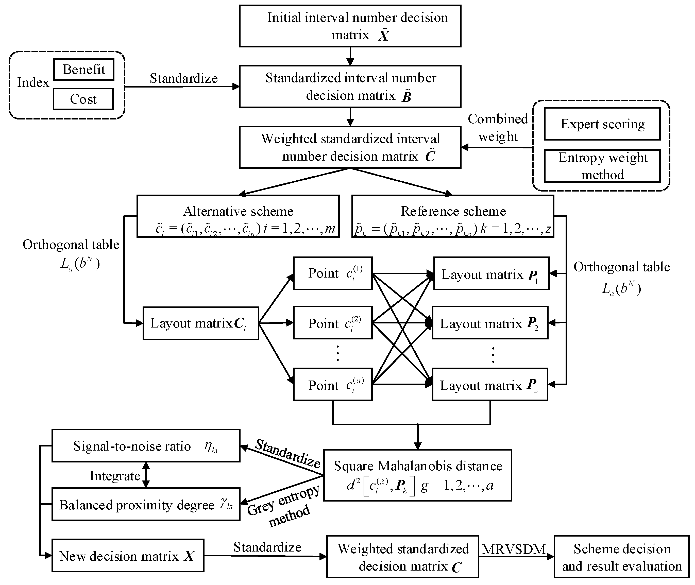
4. Multi-Dimensional Interval Number Decision Model Based on MTS-GEM

4.1. Development of the Weighted Standardized Decision Matrix

Suppose that there are m alternative schemes and n indexes, and they constitute the initial interval number decision matrix $\tilde{\mathit{X}}={\left[{\tilde{x}}_{ij}\right]}_{m\times n}$ (i=1,2,…,m; j=1,2,…,n) where ${\tilde{x}}_{ij}=\left[x_{ij}^L,x_{ij}^U\right]$. As the dimensions of the indexes are often different, we used Equations (11) and (12) to nondimensionalize different types of indexes, and get the standardized interval number decision matrix $\tilde{\mathit{B}}={\left[{\tilde{b}}_{ij}\right]}_{m\times n}$, where ${\tilde{b}}_{ij}=\left[b_{ij}^L,b_{ij}^U\right]$.

For a benefit index:

$${\tilde{b}}_{ij}=\left[\frac{x_{ij}^L-\underset{i}{\min }{x}_{ij}}{\underset{i}{\max }{x}_{ij}-\underset{i}{\min }{x}_{ij}},\frac{x_{ij}^U-\underset{i}{\min }{x}_{ij}}{\underset{i}{\max }{x}_{ij}-\underset{i}{\min }{x}_{ij}}\right],$$

(11)

For a cost index:

$${\tilde{b}}_{ij}=\left[\frac{\underset{i}{\max }{x}_{ij}-x_{ij}^U}{\underset{i}{\max }{x}_{ij}-\underset{i}{\min }{x}_{ij}},\frac{\underset{i}{\max }{x}_{ij}-x_{ij}^L}{\underset{i}{\max }{x}_{ij}-\underset{i}{\min }{x}_{ij}}\right],$$

(12)

where $\underset{i}{\min }{x}_{ij}=\min (\underset{i}{\min }{x}_{ij}^L,\underset{i}{\min }{x}_{ij}^U)$ and $\underset{i}{\max }{x}_{ij}=\max (\underset{i}{\max }{x}_{ij}^L,\underset{i}{\max }{x}_{ij}^U)$.

To make the weight distribution of each index reasonable, the integration of expert scoring (subjective weight) and entropy weight method [35] (objective weight) is used to determine the combined weight of each index.

1 Subjective weight $\tilde{\mathit{S}}={\left[{\tilde{s}}_j\right]}_{1\times n}$ where ${\tilde{s}}_j=\left[s_j^L,s_j^U\right]$

Assuming that there are $\upsilon$ experts who participate in the weight scoring of n indexes, the scoring matrix is $\tilde{\mathit{Y}}={\left[{\tilde{y}}_{lj}\right]}_{\nu \times n}$ (l=1,2,…,$\upsilon$; j=1,2,…,n) where ${\tilde{y}}_{lj}=\left[y_{\mathrm{l}j}^L,y_{\mathrm{l}j}^U\right]$, then ${\tilde{s}}_j=\left[\underset{l}{\min }{y}_{\mathrm{l}j}^L,\underset{l}{\max }{y}_{\mathrm{l}j}^U\right]$.

2 Objective weight $\tilde{\mathit{T}}=[{\tilde{t}}_j{]}_{1\times n}$, where ${\tilde{t}}_j=\left[t_j^L,t_j^U\right]$

First, the entropy of the interval number index is calculated based on the standardized interval number decision matrix $\tilde{\mathit{B}}$:

$$\begin{array}{l}{E}_j^L=-\frac{1}{\ln m}{\displaystyle {\sum }_{i=1}^m\left[\left(\frac{b_{ij}^L}{{\displaystyle {\sum }_{i=1}^m{b}_{ij}^L}}\right)\ln \left(\frac{b_{ij}^L}{{\displaystyle {\sum }_{i=1}^m{b}_{ij}^L}}\right)\right]}\\ E_j^U=-\frac{1}{\ln m}{\displaystyle {\sum }_{i=1}^m\left[\left(\frac{b_{ij}^U}{{\displaystyle {\sum }_{i=1}^m{b}_{ij}^U}}\right)\ln \left(\frac{b_{ij}^U}{{\displaystyle {\sum }_{i=1}^m{b}_{ij}^U}}\right)\right]}\end{array}$$

(13)

where $E_j^L$ and $E_j^U$ are the information entropy of the interval number index’s lower bound and upper bound, respectively; when $b_{ij}^L=0$ or $b_{ij}^U=0$, $\left(\frac{b_{ij}^L}{{\displaystyle {\sum }_{i=1}^m{b}_{ij}^L}}\right)\ln \left(\frac{b_{ij}^L}{{\displaystyle {\sum }_{i=1}^m{b}_{ij}^L}}\right)=0$ or $\left(\frac{b_{ij}^U}{{\displaystyle {\sum }_{i=1}^m{b}_{ij}^U}}\right)\ln \left(\frac{b_{ij}^U}{{\displaystyle {\sum }_{i=1}^m{b}_{ij}^U}}\right)=0$.

Then, calculate the objective weight of the interval number index ${\tilde{t}}_j$:

$${\tilde{t}}_j=\left[t_j^L,t_j^U\right]=[\min \left(\frac{1-E_j^L}{{\displaystyle {\sum }_{j=1}^n(1-E_j^L)}},\frac{1-E_j^U}{{\displaystyle {\sum }_{j=1}^n(1-E_j^U)}}\right),\max \left(\frac{1-E_j^L}{{\displaystyle {\sum }_{j=1}^n(1-E_j^L)}},\frac{1-E_j^U}{{\displaystyle {\sum }_{j=1}^n(1-E_j^U)}}\right)],$$

(14)

3 Combined weight $\tilde{\mathit{W}}=[{\tilde{w}}_j{]}_{1\times n}$, where ${\tilde{w}}_j=\left[w_j^L,w_j^U\right]$

Considering both the subjective weight $\tilde{\mathit{S}}$ and the objective weight $\tilde{\mathit{T}}$, we obtained the combined weight of the interval number index $\tilde{\mathit{W}}=[{\tilde{w}}_j{]}_{1\times n}$ where ${\tilde{w}}_j=\left[\beta s_j^L+\left(1-\beta \right)t_j^L,\beta s_j^U+\left(1-\beta \right)t_j^U\right]$ and is an empirical factor that reflects the preference of decision makers between subjective experience and objective data [36].

With the standardized decision matrix $\tilde{\mathit{B}}$ and the indexes’ combined weight $\tilde{\mathit{W}}$, we used the multiplication algorithm of interval number to obtain the weighted standardized decision matrix $\tilde{\mathit{C}}={\left[{\tilde{c}}_{ij}\right]}_{m\times n}$, where ${\tilde{c}}_{ij}={\tilde{w}}_j\times {\tilde{b}}_{ij}$. Additionally, based on TOPSIS, the positive ideal scheme ${\tilde{p}}_{+}$ and the negative ideal scheme ${\tilde{p}}_{-}$ were determined:

$$\begin{array}{l}{\tilde{p}}_{+}=\left\{\left[\underset{i}{\max }{c}_{i1}^L,\underset{i}{\max }{c}_{i1}^U\right],\left[\underset{i}{\max }{c}_{i2}^L,\underset{i}{\max }{c}_{i2}^U\right],\cdots ,\left[\underset{i}{\max }{c}_{in}^L,\underset{i}{\max }{c}_{in}^U\right]\right\}\\ {\tilde{p}}_{-}=\left\{\left[\underset{i}{\min }{c}_{i1}^L,\underset{i}{\min }{c}_{i1}^U\right],\left[\underset{i}{\min }{c}_{i2}^L,\underset{i}{\min }{c}_{i2}^U\right],\cdots ,\left[\underset{i}{\min }{c}_{in}^L,\underset{i}{\min }{c}_{in}^U\right]\right\}\end{array}$$

(15)

4.2. Orthogonal Test of Schemes and Calculation of Derivative Indicators

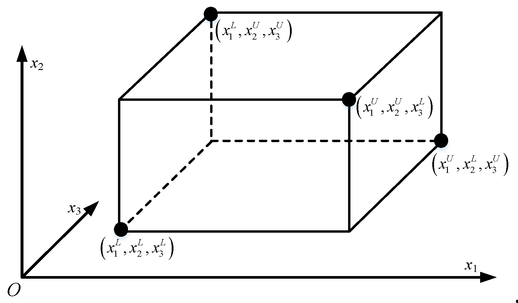
According to the number of indexes, a two-level orthogonal table with N≥n was selected, where n indexes can be arranged in any n columns. For the interval number $\tilde{a}=\left[a^L,a^U\right]$, take $a^L$ as level 1 and $a^U$ as level 2. The layout matrix ${\mathit{C}}_i$ of the alternative scheme ${\tilde{c}}_i$ (i=1,2,…,m) is as follows:

$${\mathit{C}}_i=\left[\begin{array}{l}{c}_i^{(1)}\\ c_i^{(2)}\\ ⋮\\ c_i^{(a)}\end{array}\right]={\left[\begin{array}{cccc}{c}_{i1}^{(1)}& c_{i2}^{(1)}& \cdots & c_{in}^{(1)}\\ c_{i1}^{(2)}& c_{i2}^{(2)}& \cdots & c_{in}^{(2)}\\ ⋮& ⋮& \ddots & ⋮\\ c_{i1}^{(a)}& c_{i2}^{(a)}& \cdots & c_{in}^{(a)}\end{array}\right]}_{a\times n},$$

(16)

where $c_i^{(g)}$ (g=1,2,…,a) is the distribution point of scheme ${\tilde{c}}_i$ and $c_{i1}^{(g)}$, $c_{i2}^{(g)}$, …, $c_{in}^{(g)}$ are the components of $c_i^{(g)}$.

Similarly, the layout matrix of the positive ideal scheme ${\mathit{P}}_{+}$ and the layout matrix of the negative ideal scheme ${\mathit{P}}_{-}$ can be obtained.

Here, we define derivative indicators as the signal-to-noise ratio and the degree of balance and approach based on square Mahalanobis distance obtained by the initial interval number indexes. According to Equation (6), calculate the square Mahalanobis distance between the alternative scheme’s distribution point $c_i^{(g)}$ and the positive/negative ideal scheme, and we obtain $d^2\left[c_i^{(g)},{\mathit{P}}_{+}\right]$ and $d^2\left[c_i^{(g)},{\mathit{P}}_{-}\right]$.

1 Signal-to-noise ratio

The SB signal-to-noise of the scheme i to the positive (negative) ideal scheme is ${\eta }_{+i}$ (${\eta }_{-i}$):

$$\begin{array}{l}{\eta }_{+i}=-10{\log }_{10}\left\{{\displaystyle {\sum }_{g=1}^a{d^{\prime }}^2\left[c_i^{(g)},{\mathit{P}}_{+}\right]}/a\right\}\\ {\eta }_{-i}=-10{\log }_{10}\left\{{\displaystyle {\sum }_{g=1}^a{d^{\prime }}^2\left[c_i^{(g)},{\mathit{P}}_{-}\right]}/a\right\}\end{array}$$

(17)

where a is the number of orthogonal tests and ${d^{\prime }}^2\left[c_i^{(g)},{\mathit{P}}_{+}\right]$, ${d^{\prime }}^2\left[c_i^{(g)},{\mathit{P}}_{-}\right]$ is the square Mahalanobis distance standardized by Equation (18):

$$\begin{array}{l}{d^{\prime }}^2\left[c_i^{(g)},{\mathit{P}}_{+}\right]=\frac{\underset{g}{\max }{d}^2\left[c_i^{(g)},{\mathit{P}}_{+}\right]-d^2\left[c_i^{(g)},{\mathit{P}}_{+}\right]}{\underset{g}{\max }{d}^2\left[c_i^{(g)},{\mathit{P}}_{+}\right]-\underset{g}{\min }{d}^2\left[c_i^{(g)},{\mathit{P}}_{+}\right]}\\ {d^{\prime }}^2\left[c_i^{(g)},{\mathit{P}}_{-}\right]=\frac{d^2\left[c_i^{(g)},{\mathit{P}}_{-}\right]-\underset{g}{\min }{d}^2\left[c_i^{(g)},{\mathit{P}}_{-}\right]}{\underset{g}{\max }{d}^2\left[c_i^{(g)},{\mathit{P}}_{-}\right]-\underset{g}{\min }{d}^2\left[c_i^{(g)},{\mathit{P}}_{-}\right]}\end{array}$$

(18)

2 Improved degree of balance and approach

The correlation degree of the alternative scheme ${\tilde{c}}_i$ and the positive (negative) ideal scheme is $G_{+i}$ ($G_{-i}$):

$$G_{+i}={\displaystyle {\sum }_{g=1}^a{r}_{+i}^{(g)}}/a,G_{-i}={\displaystyle {\sum }_{g=1}^a{r}_{-i}^{(g)}}/a,$$

(19)

where $r_{+i}^{(g)}$ ($r_{-i}^{(g)}$) is the correlation coefficient of the alternative scheme ${\tilde{c}}_i$ and the positive (negative) ideal scheme at distribution point g.

Based on the square Mahalanobis distance, the formula of correlation coefficient is revised as follows:

$$\begin{array}{l}{r}_{+i}^{(g)}=\frac{\underset{i}{\min }\underset{g}{\min }{d}^2\left[c_i^{(g)},{\mathit{P}}_{+}\right]+\zeta \underset{i}{\max }\underset{g}{\max }{d}^2\left[c_i^{(g)},{\mathit{P}}_{+}\right]}{d^2\left[c_i^{(g)},{\mathit{P}}_{+}\right]+\zeta \underset{i}{\max }\underset{g}{\max }{d}^2\left[c_i^{(g)},{\mathit{P}}_{+}\right]}\\ r_{-i}^{(g)}=\frac{\underset{i}{\min }\underset{g}{\min }{d}^2\left[c_i^{(g)},{\mathit{P}}_{-}\right]+\zeta \underset{i}{\max }\underset{g}{\max }{d}^2\left[c_i^{(g)},{\mathit{P}}_{-}\right]}{d^2\left[c_i^{(g)},{\mathit{P}}_{-}\right]+\zeta \underset{i}{\max }\underset{g}{\max }{d}^2\left[c_i^{(g)},{\mathit{P}}_{-}\right]}\end{array}$$

(20)

where the distinguishing coefficient $\zeta$ is set at 0.5.

The balance degree of the alternative scheme ${\tilde{c}}_i$ and the positive (negative) ideal scheme is $J_{+i}$ ($J_{-i}$):

$$\begin{array}{l}{J}_{+i}=-\frac{1}{lna}{\displaystyle {\sum }_{g=1}^a{q}_{{}_{+i}}^{(g)}ln{q}_{{}_{+i}}^{(g)}}\\ J_{-i}=-\frac{1}{lna}{\displaystyle {\sum }_{g=1}^a{q}_{{}_{-i}}^{(g)}ln{q}_{{}_{-i}}^{(g)}} \end{array}$$

(21)

where $q_{{}_{+i}}^{(g)}=r_{{}_{+i}}^{(g)}/{\displaystyle {\sum }_{g=1}^a{r}_{{}_{+i}}^{(g)}}$ and $q_{{}_{-i}}^{(g)}=r_{{}_{-i}}^{(g)}/{\displaystyle {\sum }_{g=1}^a{r}_{{}_{-i}}^{(g)}}$.

The degree of balance and approach of the alternative scheme ${\tilde{c}}_i$ and the positive (negative) ideal scheme is ${\gamma }_{+i}$ (${\gamma }_{-i}$):

$${\gamma }_{+i}=G_{+i}\times J_{+i},{\gamma }_{-i}=G_{-i}\times J_{-i},$$

(22)

4.3. Scheme Decision-Making

Based on the signal-to-noise ratio and the improved degree of balance and approach, the decision matrix Y is constructed as shown in Equation (23), in which the benefit indicator is ${\eta }_{-i}$ and ${\gamma }_{+i}$, while the cost indicator is ${\eta }_{+i}$ and ${\gamma }_{-i}$:

$$\mathit{Y}={\left[\begin{array}{cccc}{\eta }_{+1}& {\eta }_{-1}& {\gamma }_{+1}& {\gamma }_{-1}\\ {\eta }_{+2}& {\eta }_{-2}& {\gamma }_{+2}& {\gamma }_{-2}\\ ⋮& ⋮& ⋮& ⋮\\ {\eta }_{+m}& {\eta }_{-m}& {\gamma }_{+m}& {\gamma }_{-m}\end{array}\right]}_{m\times 4},$$

(23)

Now, the decision-making problem with multi-dimensional interval numbers is changed into a decision-making problem with multi-dimensional real numbers [37]. The optimal scheme can be selected with the following multi-dimensional real vector space decision-making method (MRVSDM).

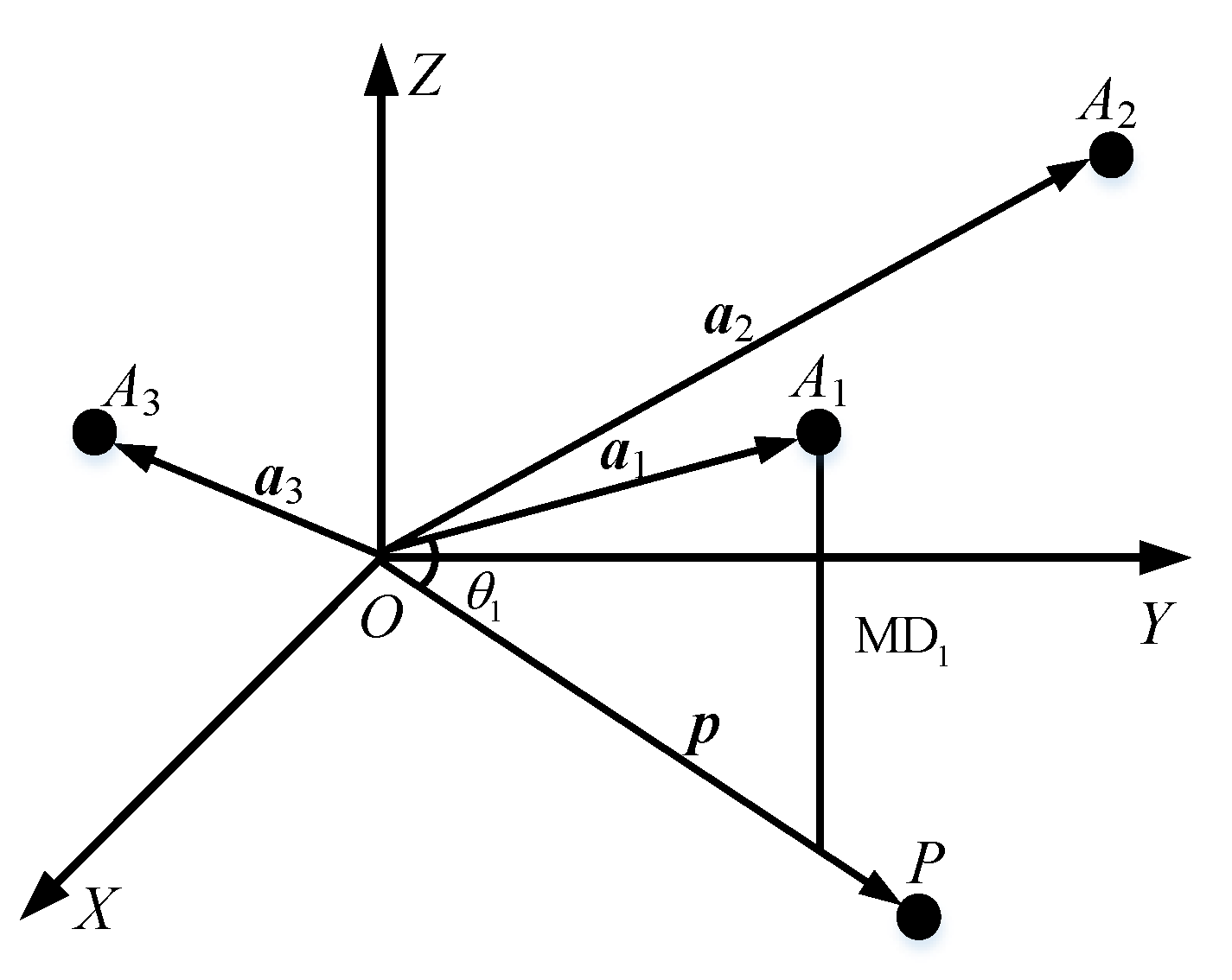
• The n-dimensional real numbers are regarded as the points A₁,…,A_i,…,A_m in an n-dimensional space with O as the origin, and then we can get the vectors ${\mathit{a}}_1={\overrightarrow{OA}}_1$,…,${\mathit{a}}_i={\overrightarrow{OA}}_i$,…,${\mathit{a}}_m={\overrightarrow{OA}}_m$.
• Assuming that the reference scheme vector is $\mathit{p}$, $\left|{\mathit{a}}_i\right|$ and $\left|\mathit{p}\right|$ are the modules of vector a_i and vector $\mathit{p}$, respectively. Between vectors a_i and $\mathit{p}$, calculate their angle ${\theta }_i=(\widehat{{\mathit{a}}_i,\mathit{p}})=\arccos \left(\frac{{\mathit{a}}_i\cdot \mathit{p}}{\left|{\mathit{a}}_i\right|\left|\mathit{p}\right|}\right)$ (where ${\mathit{a}}_i\cdot \mathit{p}$ is their product), as well as their mapping distance ${\mathrm{MD}}_i=\left|{\mathit{a}}_i\right|\mathrm{Sin}{\theta }_i$.
• The set of mapping distance $\mathrm{MD}=\left\{{\mathrm{MD}}_i|i=1,2,\cdots ,m\right\}$ can be obtained. According to the principle that the smaller ${\mathrm{MD}}_i$ is, the closer vector a_i is to vector $\mathit{p}$, the scheme that satisfies the objective $\underset{i}{\min }{\mathrm{MD}}_i$ is selected as the optimal scheme.

The diagram of decision-making in a three-dimensional real number vector space is shown in Figure 2. The input of the MTS-GEM model is the interval number indexes derived from different schemes. After orthogonal tests and calculation of the Mahalanobis distance, the signal-to-noise ratio, the improved degree of balance and approach, the output is the mapping distance from each scheme to the ideal scheme. The flow chart of this study is shown in Figure 3.

5. Case Study

5.1. Initial Interval Number Decision Matrix and Its Weighted Standardization

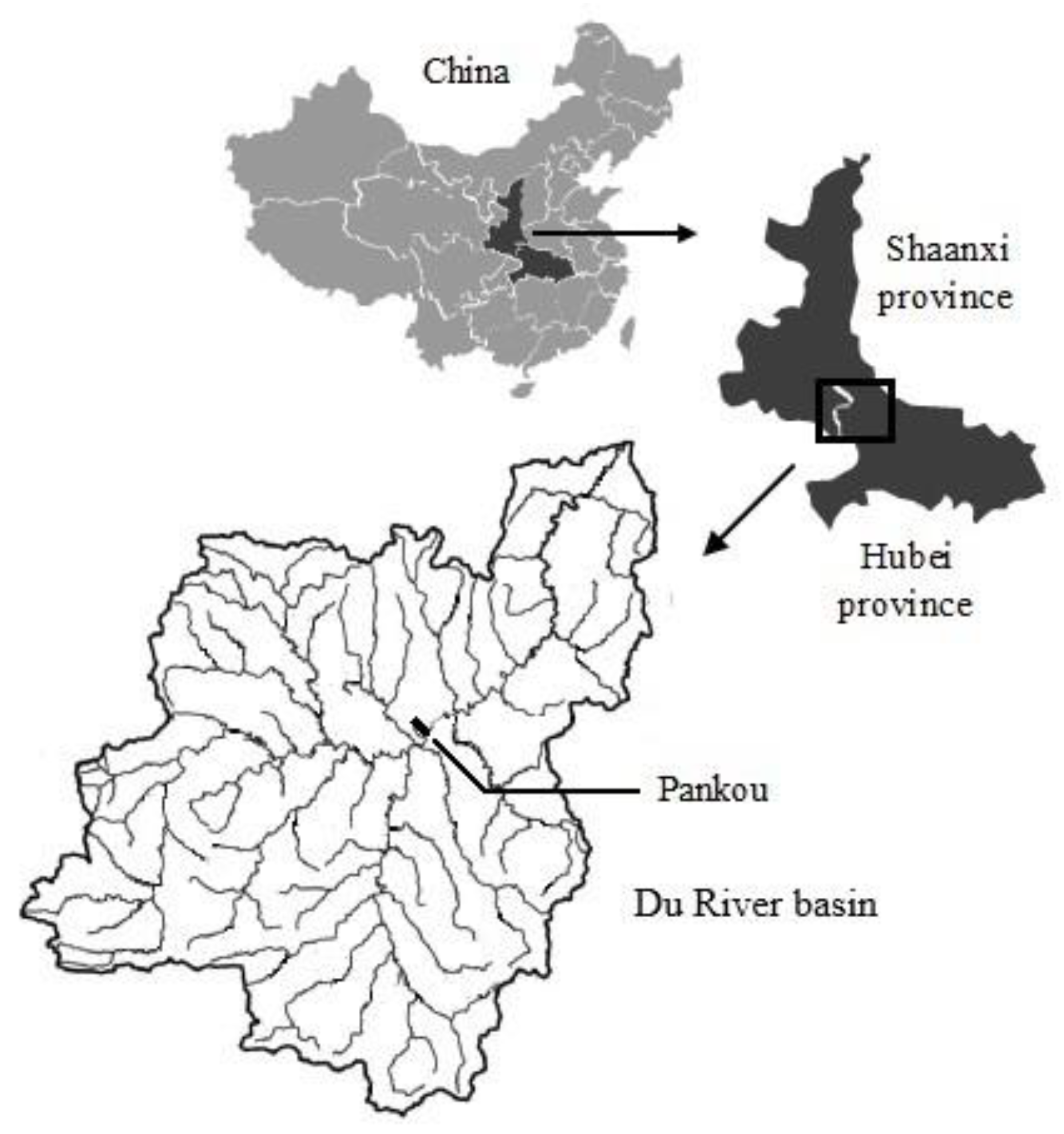
Multi-objective reservoir operation is a multi-dimensional and complicated system engineering issue. Affected by runoff forecast, operation model, solution method and other factors, in the obtained non-inferior solution set, the attribute values are not always a precise real number but an interval number with uncertainty. The Pankou reservoir, located at the upstream of the Du River in China, is an annual-regulating reservoir with comprehensive utilization tasks of power generation, flood control, water supply and so forth. Its basic information is listed in

Table 3. Basic information of the Pankou reservoir.

Item	Unit	Pankou
Dead water level	m	330
Flood control limit water level	m	347.6
Normal water level	m	355
Flood control high water level	m	358.4
Design flood water level	m	357.14
Spillway flood water level	m	360.82
Minimum storage capacity	108 m3	8.5
Regulating storage capacity	108 m3	11.2
Total storage capacity	108 m3	23.38
Regulating performance	–	Annual regulating
Installed power capacity	MW	500
Average annual generated power	108 kW·h	10.474

, and its location map is shown in Figure 4.

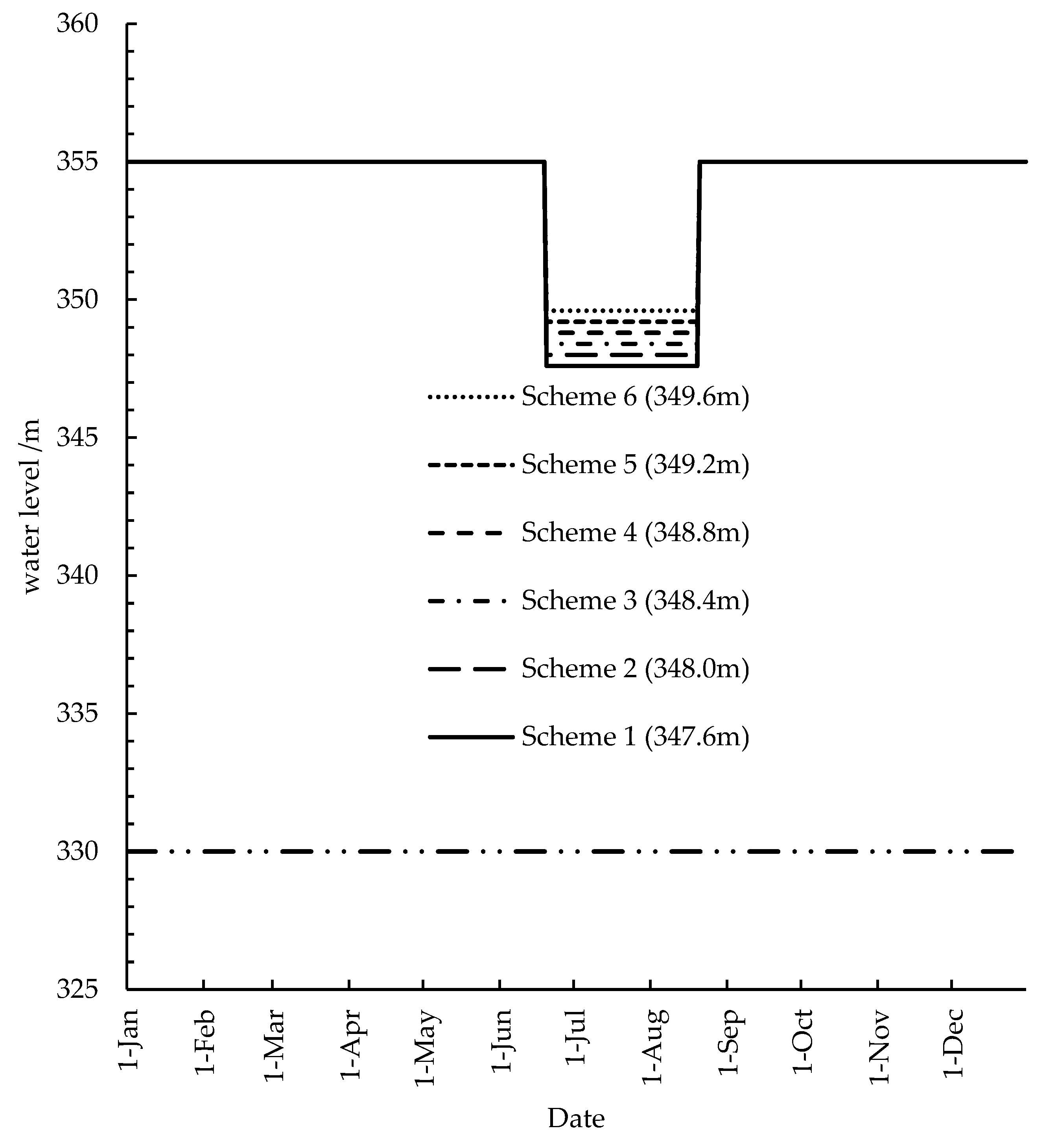
According to the current regulations of the China Yangtze River Flood Control and Drought Relief Headquarters, for the Pankou reservoir, the upper limit of operation water level in flood season (June 20–August 20) is the flood control limit water level (347.6 m), while in other periods it is the normal water level (355 m); the lower limit of operation water level in all periods is the dead water level (330 m), and falling to the lower limit should be avoided during operation.

However, in the actual operation of the Pankou reservoir, it can barely store water to the normal water level in most years, undermining such benefits as power generation and water supply. In order to reasonably adjust the upper limit of water level in flood season and improve the utilization rate of flood resources, in reference [38] the three indexes of flood control risk rate, annual generated power and water storage at the end of flood season were used as the evaluation indexes for selecting the optimal scheme of water level upper limit in flood season. Flood control risk rate was obtained by means of flood stochastic simulation [39]. Firstly, the flood stochastic simulation model was used to simulate n (a large number) pieces of annual maximum flood inflow hydrographs, which can fully reflect the statistical characteristics of the reservoir’s measured flood inflow. Then, a flood operation calculation was conducted to obtain the highest annual water level sequence, and the ratio of times that the water level limit was exceeded to n was taken as the flood control risk rate, the value of which needs to meet people’s acceptable level of risk. Annual generated power refers to the total electricity generated by the hydropower station within a one-year operation cycle, which represents the power generation benefit of the hydropower station. The more annual generated power, the greater the annual power generation benefit. The water storage at the end of the flood season refers to the water storage between the dead water level and the particular water level at the end of flood season, which represents the water supply benefit of the reservoir. The more water storage at the end of flood season, the greater the water supply benefit.

The scheme setting is shown in Figure 5. Currently, Scheme 1 is being adopted as the operation strategy of the Pankou reservoir’s upper water level limit in flood season.

For the flood control risk rate, the Monte Carlo method was used to randomly simulate 100 groups of 1000 floods corresponding to the 1000-year return period (0.1%). After flood operation calculation of each flood, the number of times that the design flood water level (357.14m) is exceeded in each group of 1000 floods were counted as ${\lambda }_{\xi }(\xi =1,2,\cdots ,100)$. The flood control risk rate of each group was ${\lambda }_{\xi }/1000$, and the flood control risk rate in the form of an interval number was $\left[\underset{1⩽\xi ⩽100}{\min }\left({\lambda }_{\xi }/1000\right),\underset{1⩽\xi ⩽100}{\max }\left({\lambda }_{\xi }/1000\right)\right]$. Similarly, the annual generated power and water storage at the end of flood season were obtained through reservoir operation calculation by using the monthly inflow data of 41 years from 1971 to 2011. Then, the minimum and maximum values of the 41 results formed the interval numbers. The initial interval number decision matrix $\tilde{\mathit{X}}$ is shown in

Table 4. Initial interval number decision matrix $\tilde{\mathit{X}}$.

Scheme i	$\mathbf{Flood} \mathbf{Control} \mathbf{Risk} \mathbf{Rate} {\tilde{\mathit{x}}}_{\mathit{i}1}/ \%$	$\mathbf{Annual} \mathbf{Generated} \mathbf{Power} {\tilde{\mathit{x}}}_{\mathit{i}2}/{10}^8 \mathbf{kW}·\mathbf{h}$	$\mathbf{Water} \mathbf{Storage} \mathbf{at} \mathbf{the} \mathbf{End} \mathbf{of} \mathbf{Flood} \mathbf{Season} {\tilde{\mathit{x}}}_{\mathit{i}3}/{10}^8 {\mathbf{m}}^3$
1	[1.812,4.371]	[6.531,14.392]	[4.887,11.200]
2	[1.882,4.408]	[7.086,14.983]	[5.411,11.200]
3	[1.993,4.421]	[7.687,15.639]	[6.033,11.200]
4	[2.211,4.689]	[8.275,16.136]	[6.751,11.200]
5	[2.534,5.028]	[8.699,16.641]	[7.523,11.200]
6	[2.977,5.594]	[9.320,17.343]	[8.431,11.200]

.

According to Equation (11)–(12), the benefit indexes (annual generated power, water storage at the end of flood season) and the cost index (flood control risk rate) in Table 3 are standardized, resulting in the standardized interval number decision matrix $\tilde{\mathit{B}}$ shown in

Table 5. Standardized interval number decision matrix $\tilde{\mathit{B}}$.

Scheme i	$\mathbf{Flood} \mathbf{Control} \mathbf{Risk} \mathbf{Rate} {\tilde{\mathit{b}}}_{\mathit{i}1}$	$\mathbf{Annual} \mathbf{Generated} \mathbf{Power} {\tilde{\mathit{b}}}_{\mathit{i}2}$	$\mathbf{Water} \mathbf{Storage} \mathbf{at} \mathbf{the} \mathbf{End} \mathbf{of} \mathbf{Flood} \mathbf{Season} {\tilde{\mathit{b}}}_{\mathit{i}3}$
1	[0.323,1.000]	[0.000,0.727]	[0.000,1.000]
2	[0.314,0.981]	[0.051,0.782]	[0.083,1.000]
3	[0.310,0.952]	[0.107,0.842]	[0.182,1.000]
4	[0.239,0.895]	[0.161,0.888]	[0.295,1.000]
5	[0.150,0.809]	[0.201,0.935]	[0.418,1.000]
6	[0.000,0.692]	[0.258,1.000]	[0.561,1.000]

.

According to Lynne [40] who derives the variance formula of interval number sample matrix based on uniform distribution, for $\tilde{\mathit{B}}={\left[{\tilde{b}}_{ij}\right]}_{m\times n}$, its variance $D({\tilde{b}}_j)$ can be expressed as follows:

$$D({\tilde{b}}_j)=\frac{1}{3m}{\displaystyle {\sum }_{i=1}^m\left[{(b_{ij}^L)}^2+b_{ij}^L{x}_{ij}^U+{(b_{ij}^U)}^2\right]}-\frac{1}{4m^2}{\left[{\displaystyle {\sum }_{i=1}^m(b_{ij}^L+b_{ij}^U)}\right]}^2,$$

(24)

Based on the definition of the correlation coefficient of two random real number variables in the probability theory and mathematical statistics, the correlation coefficient of two interval variables $\rho ({\tilde{b}}_h,{\tilde{b}}_j)$ (h, j=1,2,…,n) is:

$$\rho ({\tilde{b}}_h,{\tilde{b}}_j)=\frac{\mathrm{Cov}({\tilde{b}}_h,{\tilde{b}}_j)}{\sqrt{D({\tilde{b}}_h,)}\sqrt{D({\tilde{b}}_j)}}=\frac{D({\tilde{b}}_h+{\tilde{b}}_j)-D({\tilde{b}}_h)-D({\tilde{b}}_j)}{2\sqrt{D({\tilde{b}}_h)}\sqrt{D({\tilde{b}}_j)}},$$

(25)

From Equation (24)–(25), the correlation coefficient matrix of $\tilde{\mathit{B}}={\left[{\tilde{b}}_{ij}\right]}_{m\times n}$ can be obtained, as shown in

Table 6. Correlation coefficient matrix of the standardized interval number decision matrix.

Index	$\mathbf{Flood} \mathbf{Control} \mathbf{Risk} \mathbf{Rate} {\tilde{\mathit{b}}}_1$	$\mathbf{Annual} \mathbf{Generated} \mathbf{Power} {\tilde{\mathit{b}}}_2$	$\mathbf{Water} \mathbf{Storage} \mathbf{at} \mathbf{the} \mathbf{End} \mathbf{of} \mathbf{Flood} \mathbf{Season} {\tilde{\mathit{b}}}_3$
Flood control risk rate ${\tilde{b}}_1$	1.000	0.613	0.573
Annual generated power ${\tilde{b}}_2$	0.613	1.000	0.971
Water storage at the end of flood season ${\tilde{b}}_3$	0.573	0.971	1.000

.

It is shown in Table 5 that there is positive correlation among the three indexes. The correlation between the flood control risk rate and annual generated power or water storage at the end of flood season is slightly weak. The correlation between annual generated power and water storage at the end of flood season is significant in that their correlation coefficient is 0.971. Thus, it is necessary to consider the correlation between the indexes in the decision-making process of the reservoir water level scheme in flood season.

There are five experts to grade the importance of the indexes, and the subjective weight of the interval number indexes obtained from the scoring matrix is $\tilde{\mathit{S}}=\left\{\left[0.320,0.397\right] \left[0.292,0.360\right] \left[0.235,0.300\right]\right\}$. According to Equation (13), the information entropy weight is $t_j^L=(0.252,0.347,0.401)$ and $t_j^U=(0.573,0.427,0)$. Thus, the objective weight of the interval number indexes is $\tilde{\mathit{T}}=\left\{\left[0.252,0.573\right] \left[0.347,0.427\right] \left[0,0.401\right]\right\}$. Let the empirical factor $\beta$ be 0.5, then the combined weight is $\tilde{\mathit{W}}=\left\{\left[0.286,0.485\right] \left[0.320,0.394\right] \left[0.118,0.351\right]\right\}$. From $\tilde{\mathit{B}}$ and $\tilde{\mathit{W}}$, the weighted standardized decision matrix $\tilde{\mathit{C}}$ is obtained, as shown in

Table 7. Weighted standardized interval number decision matrix $\tilde{\mathit{C}}$.

Scheme i	$\mathbf{Flood} \mathbf{Control} \mathbf{Risk} \mathbf{Rate} {\tilde{\mathit{c}}}_{\mathit{i}1}$	$\mathbf{Annual} \mathbf{Generated} \mathbf{Power} {\tilde{\mathit{c}}}_{\mathit{i}2}$	$\mathbf{Water} \mathbf{Sstorage} \mathbf{at} \mathbf{the} \mathbf{End} \mathbf{of} \mathbf{Flood} \mathbf{Season} {\tilde{\mathit{c}}}_{\mathit{i}3}$
1	[0.092, 0.485]	[0.000, 0.286]	[0.000, 0.351]
2	[0.090, 0.476]	[0.016, 0.308]	[0.010, 0.351]
3	[0.089, 0.462]	[0.034, 0.332]	[0.021, 0.351]
4	[0.068, 0.434]	[0.052, 0.350]	[0.035, 0.351]
5	[0.043, 0.392]	[0.064, 0.368]	[0.049, 0.351]
6	[0.000, 0.336]	[0.083, 0.394]	[0.066, 0.351]

.

Through the matrix $\tilde{\mathit{C}}$, based on TOPSIS and Equation (15), the positive (negative) ideal scheme ${\tilde{p}}_{+}$ (${\tilde{p}}_{-}$) is determined as follows:

${\tilde{p}}_{+}=\left\{\left[0.092,0.485\right] \left[0.083,0.394\right] \left[0.066,0.351\right]\right\}$

${\tilde{p}}_{-}=\left\{\left[0.000,0.336\right] \left[0.000,0.286\right] \left[0.000,0.351\right]\right\}$.

5.2. Orthogonal Test of the Schemes

Since there are three indexes, the orthogonal table is $L_4(2^3)$. The alternative scheme’s layout matrix C_i (i=1,2,…,6), the positive ideal scheme’s layout matrix ${\mathit{P}}_{+}$ and the negative ideal scheme’s layout matrix ${\mathit{P}}_{-}$ are shown in

Table 8. Layout matrixes of the schemes.

Matrix	Flood Control Risk Rate	Annual Generated Power	Water Storage at the End of Flood Season	Matrix	Flood Control Risk Rate	Annual Generated Power	Water Storage at the End of Flood Season
C1	0.092	0.000	0.000	C5	0.043	0.064	0.049
	0.092	0.286	0.351		0.043	0.368	0.351
	0.485	0.000	0.351		0.392	0.064	0.351
	0.485	0.286	0.000		0.392	0.368	0.049
C2	0.090	0.016	0.010	C6	0.000	0.083	0.066
	0.090	0.308	0.351		0.000	0.394	0.351
	0.476	0.016	0.351		0.336	0.083	0.351
	0.476	0.308	0.010		0.336	0.394	0.066
C3	0.089	0.034	0.021	${\mathit{P}}_{+}$	0.092	0.083	0.066
	0.089	0.332	0.351		0.092	0.394	0.351
	0.462	0.034	0.351		0.485	0.083	0.351
	0.462	0.332	0.021		0.485	0.394	0.066
C4	0.068	0.052	0.035	${\mathit{P}}_{-}$	0.000	0.000	0.000
	0.068	0.350	0.351		0.000	0.286	0.351
	0.434	0.052	0.351		0.336	0.000	0.351
	0.434	0.350	0.035		0.336	0.286	0.000

.

5.3. Scheme Decision-Making and Result Evaluation

The square Mahalanobis distance from each point in the layout matrix C_i to the positive ideal scheme’s layout matrix ${\mathit{P}}_{+}$ and the negative ideal scheme’s layout matrix ${\mathit{P}}_{-}$ is worked out, as shown in

Table 9. Square Mahalanobis distance.

Scheme i	${\mathit{d}}^2\left[{\mathit{c}}_{\mathit{i}}^{(\mathit{g})},{\mathit{P}}_{+}\right]$				${\mathit{d}}^2\left[{\mathit{c}}_{\mathit{i}}^{(\mathit{g})},{\mathit{P}}_{-}\right]$
1	4.139	1.567	3.263	2.428	1.658	1.649	4.166	4.175
2	3.774	1.662	2.966	2.290	1.424	1.906	3.858	4.190
3	3.386	1.790	2.630	2.155	1.187	2.222	3.478	4.192
4	3.152	2.076	2.238	1.909	1.054	2.583	2.930	3.936
5	3.071	2.436	1.901	1.668	1.037	3.018	2.308	3.583
6	3.132	3.112	1.542	1.543	1.177	3.806	1.628	3.355

.

The square Mahalanobis distance is standardized by Equation (18) and the SNR indicator is obtained. The indicator of the degree of balance and approach is worked out by Equation (19)–(22). Accordingly, the decision matrix X is derived, as shown in

Table 10. Derivative indicator decision matrix X.

Scheme i	${\mathit{\eta }}_{+\mathit{i}}$	${\mathit{\eta }}_{-\mathit{i}}$	${\mathit{\gamma }}_{+\mathit{i}}$	${\mathit{\gamma }}_{-\mathit{i}}$
1	2.998	3.010	0.753	0.652
2	2.829	2.894	0.775	0.660
3	2.508	2.784	0.801	0.669
4	1.869	2.633	0.824	0.686
5	2.429	2.446	0.841	0.705
6	2.984	3.010	0.838	0.710

.

In accordance with Equation (11)–(12), X is standardized and with the weight of each index being 0.25, the weighted standardized decision matrix C is obtained, as shown in

Table 11. Weighted standardized derivative indicator decision matrix C.

Scheme i	${\mathit{\eta }}_{+\mathit{i}}^{\ast }$	${\mathit{\eta }}_{-\mathit{i}}^{\ast }$	${\mathit{\gamma }}_{+\mathit{i}}^{\ast }$	${\mathit{\gamma }}_{-\mathit{i}}^{\ast }$
1	0.000	0.250	0.000	0.250
2	0.037	0.199	0.063	0.216
3	0.109	0.150	0.136	0.177
4	0.250	0.083	0.202	0.103
5	0.126	0.000	0.250	0.022
6	0.003	0.250	0.241	0.000

.

$p=\left[0.25,0.25,0.25,0.25\right]$ is taken as the reference scheme to calculate the mapping distance ${\mathrm{MD}}_i$ from the alternative scheme to the reference scheme.

To verify the feasibility and effectiveness of the method in this paper, the first comparison method of scheme ranking (method 1) is based on the closeness degree of the SNR defined by Equation (26), according to reference [40]:

$${\eta }_i=\frac{{\eta }_{-i}}{{\eta }_{+i}+{\eta }_{-i}},$$

(26)

On the basis of TOPSIS, the improved closeness degree of the degree of balance and approach is defined as follows:

$${\gamma }_i=\frac{{\gamma }_{+i}}{{\gamma }_{+i}+{\gamma }_{-i}},$$

(27)

When ${\gamma }_{-i}\to 0$, ${\gamma }_i\to 1$, the closer scheme i is to the positive ideal scheme, whereas when ${\gamma }_{+i}\to 0$, ${\gamma }_i\to 0$, the farther scheme i is to the positive ideal scheme. This ranking criterion is that the larger ${\gamma }_i$ is, the better the corresponding scheme i is, which is the second method for comparison (method 2).

The schemes are sorted according to the different ranking criteria of method 1, method 2 and the method in this study. The results are shown in

Table 12. Results of scheme ranking.

Scheme i	Method 1		Method 2		This Study’s Method
	${\mathit{\eta }}_{\mathit{i}}$	Ranking	${\mathit{\gamma }}_{\mathit{i}}$	Ranking	${\mathit{MD}}_{\mathit{i}}$	Ranking
1	0.5010	6	0.5359	6	0.2500	6
2	0.5057	3	0.5401	5	0.1585	3
3	0.5260	2	0.5449	2	0.0492	1
4	0.5848	1	0.5457	1	0.1378	2
5	0.5018	5	0.5440	3	0.1983	4
6	0.5021	4	0.5413	4	0.2443	5

.

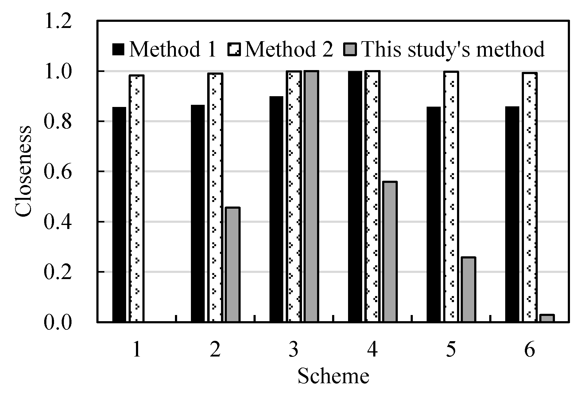
It can be seen from Table 11 that Scheme 1 ranks the last in the decision results of all the three methods, meaning that the currently-adopted strategy is far from decent and other schemes need to be selected, which conforms to the status quo of the Pankou reservoir. This study’s method chooses Scheme 3 as the optimal scheme, which raises the upper water level limit in flood season by 0.8 m compared with Scheme 1.

The reasons for the inconsistent scheme ranking results can be explained by the calculation process of the SNR and the improved degree of balance and approach in Section 4.2. The two indicators respectively reflect the output strength and the degree of balance and approach of geometric curves in the alternative and the reference schemes. If method 1 or method 2 is used alone, their decision results will be less likely to be adopted. The method proposed in this paper includes the advantages of both method 1 and method 2, and gets closer to the reference scheme by the mapping distance, producing more accurate and reasonable decision results. Therefore, scheme 3 is recommended as the optimal.

In Table 11, the closeness degree of the SNR and the closeness degree of the balance and approach degree are benefit indicators, whereas the mapping distance is a cost indicator, and therefore converted into a benefit indicator by the range method. After normalizing the three indicators, the decision results of the three methods are illustrated in Figure 6. It can be seen that compared with method 1 and method 2, this study’s method produces more obviously distinct decision results, which proves that the proposed model can effectively mine the hidden rules in data, especially for the analysis of a system with deficient information.

6. Conclusions

In order to reduce the uncertainty of interval numbers as well as computation work and fully mine the implied information in multi-attribute decision-making, a multi-dimensional interval number decision model based on Mahalanobis-Taguchi System with grey entropy method (MTS-GEM) was proposed and verified by a case study. The principal conclusions are as follows.

• MTS-GEM can effectively reduce the uncertainty created by interval numbers. In the model, the bounded uncertain n-dimensional interval number is expressed quantitatively as a hypercube in the n-dimensional space. Meanwhile, the alternative and reference schemes are all transformed into finite vertices of the hypercube, which realizes the transformation from an interval number decision vector to a real number decision vector.
• MTS-GEM can produce markedly distinctive decision results, which demonstrates the sufficiency of decision information contained in the model. The model not only considers the output response strength and the degree of balance and approach between alternative and reference schemes, but also uses the idea of further approaching the reference scheme by mapping distance, which elevates the accuracy and reliability of the decision results.
• The case study of selecting the optimal scheme of controlling the Pankou reservoir’s water level in flood season shows that the proposed method can pick out the best scheme that better coordinates risk and benefit, which further proves the comprehensive and excellent decision-making performance of the model.