Cyanobacterial Blooms in Lake Varese: Analysis and Characterization over Ten Years of Observations

Abstract

Cyanobacteria blooms are a worldwide concern for water bodies and may be promoted by eutrophication and climate change. The prediction of cyanobacterial blooms and identification of the main triggering factors are of paramount importance for water management. In this study, we analyzed a comprehensive dataset including ten-years measurements collected at Lake Varese, an eutrophic lake in Northern Italy. Microscopic analysis of the water samples was performed to characterize the community distribution and dynamics along the years. We observed that cyanobacteria represented a significant fraction of the phytoplankton community, up to 60% as biovolume, and a shift in the phytoplankton community distribution towards cyanobacteria dominance onwards 2010 was detected. The relationships between cyanobacteria biovolume, nutrients, and environmental parameters were investigated through simple and multiple linear regressions. We found that 14-days average air temperature together with total phosphorus may only partly explain the cyanobacteria biovolume variance at Lake Varese. However, weather forecasts can be used to predict an algal outbreak two weeks in advance and, eventually, to adopt management actions. The prediction of cyanobacteria algal blooms remains challenging and more frequent samplings, combined with the microscopy analysis and the metagenomics technique, would allow a more conclusive analysis.

1. Introduction

Cyanobacteria are photosynthetic bacteria that occur naturally in fresh, brackish, marine waters, and terrestrial environments [1]. Cyanobacteria are a worldwide problem [2] for their ability to form massive blooms that can produce a wide range of harmful toxins [3]. Bloom events are likely to be promoted by eutrophication and climate change, and the number and intensity of these blooms increased globally over the last decades [4]. Cyanobacteria can cause a whole range of problems for human health and the environment. Fish killed by anoxia caused by the decay of the cyanobacteria biomass is a notorious effect of cyanobacteria blooms [5]. Moreover, in some conditions, cyanobacteria can produce cyanotoxins (that includes hepatotoxins, neurotoxins, cytotoxins, and dermotoxins) negatively impacting the survival of aquatic organisms [6]. In addition to wild animals, intoxication can also occur for domestic animals and humans, either by direct ingestion of cyanobacteria cells and/or through consumption of drinking water containing cyanotoxins [7], leading to public health concerns [3]. Cyanobacteria blooms also generate bad-smelling mucilaginous scum that both impact the recreational use of water bodies and prevent their use for drinking water. Considering the negative impacts of cyanobacterial blooms on ecological, economical, and human health, their monitoring and forecast is of paramount importance for lake management [8]. Several monitoring approaches and predictive models were developed to provide accurate and timely information regarding the development of cyanobacterial bloom in the waterbodies.

Different modeling techniques are known and used for algal bloom prediction, the most common being multiple linear regression (MLR) and artificial neural networks (ANNs). MLR is the simplest technique used to develop linear models and used, for example, to predict cyanobacteria [9,10] or chlorophyll-a [11,12,13] abundance, while ANNs are complex machine learning techniques, which mimic the neural adaptation behavior in order to “learn” how to solve a problem.

Eutrophication has been cited as a major cause of increasing harmful cyanobacterial/algal blooms, in particular in the Mediterranean area [14], and factors including light, temperature, quiescent water and nutrients, mainly total nitrogen (TN) and total phosphorus (TP), are considered among the main drivers of cyanobacterial blooms [15,16]. Albeit, it is well known that important predictors for cyanobacteria dominance and biomass are TP and TN [17,18], there are increasing evidences that water temperature (WT) is an important factor [9,19,20,21,22,23,24]. Warming waters intensify the vertical stratification and lengthen the period of seasonal stratification, which is one of the main physical variables determining the occurrence of algal bloom outbreaks [25]. The most evident effect of stratification is the changing availability of nutrients, which may be accumulated in surface layers or mixed in the entire water column. The increasing global air temperature may increase the strength and depth of stratification, with possible influences on the seasonal timing and changes in the phytoplankton phenology and community succession. Stratification leads cyanobacteria to outcompete other phytoplankton groups, both because of their buoyancy regulation ability [26,27] and because cyanobacteria are positively affected by the increase of water temperature [22]. In addition, it has been shown that the meteorological variables as air temperature, wind speed, and relative humidity, could be drivers of hypolimnetic anoxia, which is an indirect consequence of thermal stratification [28].

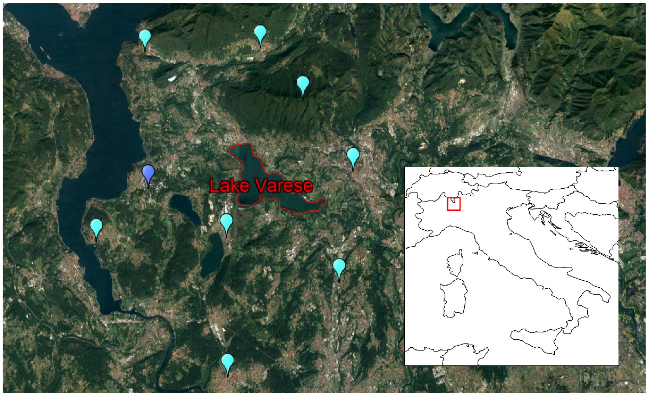
Previous studies found conflicting results on the response of cyanobacteria to climate and nutrients [23,29]. Here, we aim to identify the most important and efficient predictor for cyanobacteria blooms in Lake Varese, an eutrophic lake in northern Italy and one of the first and most glaring examples of eutrophication in Europe [30]. Initially classified as hypertrophic lake, following remedial actions aimed at reduction of the P loading, the lake is now in eutrophic status with bloom events occurring every year during the summer and early autumn. Lake Varese is “naturally productive” due to its morphometric characteristics and the geology of its drainage basin [31]. However, the further increase of human activities in the area accelerated the degradation of its water quality. The analysis of carotenoid stratigraphy of the sediments showed also that some phytoplanktonic groups are particularly well adapted in environments with high organic content.

The first signals of summer anoxia in the Lake were documented in 1957 and the fishery activities ended in 1975 [32]. Albeit, many studies testified the deterioration of the water quality, phytoplankton studies in Lake Varese were carried out only occasionally [33]. The first detailed analysis dates back to 1979 [34] and ten years later a further comprehensive study [35] showed that the eutrophication process was not showing any sign of reversion, and that the P release from sediments is a major factor constraining the recovery of lake ecosystems [36].

In this study, we firstly analyzed the cyanobacteria community with a detailed ten-year picture of the dynamic composition. We further explored the possible role of chemical and physical parameters triggering cyanobacteria blooms, introducing a novel approach to find possible relationships between meteorological data, lake stratification, and cyanobacteria abundance. We developed a simple approach that can be applied to other lakes using relatively few data and weather forecast data to put in place an early warning system for cyanobacteria blooms.

2. Materials and Methods

2.1. Sites Description

The selected study area is Lake Varese (45° 49’ N 8° 44’ E), which is located in northern Italy at the feet of the Alps mountain range at a mean altitude of 236 m above sea level (Figure 1). Lake Varese is a monomictic and eutrophic shallow lake, with a mean depth of 11 m, a maximum depth of 26 m, a surface area of 14.8 km², a volume of 153 × 106 m³, and a theoretical renewal time of 1.7–1.9 years [37,38]. Its catchment, with a surface area of 115.5 km², hosts an average population density of 700 inhabitant/km² and is associated with many industrial and commercial activities. The lake has two tributaries: The Brabbia channel and the Tinella stream, with annual average discharges of 23 × 10⁶ and 10 × 10⁶ m³ yr⁻¹, respectively, and one effluent, the Bardello stream, with annual average discharge of 80.4 × 10⁶ m³ yr⁻¹ [30]. Information related to watershed characteristics of Lake Varese can be retrieved at the following link: https://www.regione.lombardia.it/wps/portal/istituzionale/HP/aqst-lago-di-varese/documenti-e-atti-istitutivi.

2.2. Sampling and Analysis

Physical, chemical, and phytoplankton measurements of Lake Varese were provided by the department of the Regional Environmental Protection Agency of Lombardia (ARPA). The samplings were performed at least six times a year, as foreseen in the national reference methods [39], by using the multiprobe (Ocean Seven 316 plus, IDRONAUT) to measure pH, conductivity, redox potential, photosynthetically active radiation (PAR), oxygen, depth, and temperature. Water transparency was determined using a Secchi disk. The euphotic region was determined as 2.5 times the Secchi disk depth or the region where PAR was larger than 1% of the radiation determined immediately below the water surface, and applied for the collection of integrated samples used for phytoplankton analysis.

The complete dataset is composed of 90 sampling campaigns distributed over ten years, from 2004 to 2014, including measures of chemical and physical parameters of lake water sampled at different depths in the euphotic zone. Measurements of nutrients and other chemical parameters were reported at only three depths (surface, 13 m and bottom) until 2011, while from 2012 they were also reported at 4/5 of the epilimnium. This vertical resolution is rather coarse to analyze the vertical stratification of these parameters and for this reason we only provide an overview of these data by reporting mean values and their ranges (minimum and maximum). In general, the concentrations of nutrients (phosphorus and nitrogen) and oxygen are related to the presence of cyanobacteria blooms (i.e., nitrogen compounds and phosphorus are consumed/depleted from the surface while oxygen is enriched due to photosynthesis).

Table 1. List of water surface physical–chemical variables and total cyanobacteria biovolume/density measured at Lake Varese during the period 2004–2014. The mean, median, and range (minimum–maximum) values are reported for each variable. The number of samples above and below the level of quantification (LOQ), and missing values are reported. The number of cyanobacteria (present/absent) over the total sampling campaigns is shown.

Parameter and Unit of Measures		Mean	Median	Range	Above LOQ	Below LOQ	Missing
Total phosphorous (µg/L)	(TP)	42.3	28	2.5–110	80	9	1
Ammonium nitrogen (mg/L)	(AN)	0.12	0.048	0.0075–0.69	75	14	1
Reactive silicates (SiO2) (mg/L)	(RS)	1.16	0.92	0.05–3.9	82	6	2
pH	(pH)	8.18	8.2	7.5–9.6	90	0	0
Conductivity (µS/cm 20 °C)	(CD)	257	258	175–310	90	0	0
Dissolved oxygen (mg/L)	(DO)	9.64	9.8	3.7–14.8	87	0	3
Oxygen saturation (%)	(OS)	101	100	50–173	88	0	2
Water temperature (°C)	(WT)	16.3	18	3.6–30	89	0	1
Secchi disk depth (m)	(SD)	4.1	3.6	1.1–9.6	90	0	0
		Mean	Median	Range	Present	Absent
Cyanobacteria biovolume (mm3/m3)	(CyanoBV)	1.62 × 103	3.05 × 102	0–3.94 × 104	83	7
Cyanobacteria density (cells/L)	(CyanoD)	9.69 × 106	3.62 × 105	0–1.26 × 108	84	6

summarizes the physical–chemical parameters with a sufficient number of valid measurements used for this study. All parameters with missing values or below the limit of quantification (LOQ) for more than 20% of the samples were excluded. For the remaining variables, values below LOQ were arbitrarily halved, resulting in a preliminary list of nine potential variables for modeling cyanobacteria abundance. The variables may be all related, directly or indirectly, to the abundance of cyanobacteria and include both nutrient concentrations (such as: Total phosphorus, TP; ammonium nitrogen, AN; and reactive silicates, RS) and physical parameters (such as: Water temperature, WT; pH; conductivity, CD; dissolved oxygen, DO; oxygen saturation, OS; and Secchi disk depth, SD). Total nitrogen (TN) was not calculated, therefore this parameter is not available in the dataset.

Phytoplakton Analysis

Collected samples were fixed with a Lugol Acid solution and stored in the dark until analysis was performed. Phytoplankton community was evaluated according to Utermöhl’s method [40]. Shortly, a fixed sample was placed on a sedimentation tower during 24 h before microscopy analysis (Olympus model IX71 with 200X and 400X magnification). For each sample a minimum of 200 cells were identified to the genus or species level and enumerated to determine cell density. Biovolume was calculated using geometric similar models for each identified cell [41].

Cyanobacteria were measured at the level of genera/species as cell densities (cells/L) and biovolumes (mm³/m³), measured as integrated samples from the surface to 2.5 times the SD (considered as the limit of the euphotic zone). The total cyanobacteria cell density (CyanoD) and biovolume (CyanoBV) was calculated as the sum of all reported genera/species for each sampling date. Due to the large range of measured total biovolumes, spanning over several order of magnitudes, we applied the log based 10 transformation to predict the cyanobacteria biovolume (LOG CyanoBV). Variability associated with multiple cell counters could be present, however, a Phytoplankton Proficiency Test organized by EQAT Phytoplankton (External Quality Assessment Trials) was successfully completed in 2013 and 2016.

2.3. Meteorological Data

The meteorological data were obtained from the European Centre Medium-Range Weather Forecast (ECMWF) ERA-Interim atmospheric reanalysis product [42]. The reanalysis is a global model simulation of the atmosphere with a data assimilation system which includes a 4-dimensional variational analysis (4D-var). A large number of atmospheric observations, ground-based and from satellites, are included in the model variational analysis every 12 h, constraining the atmospheric weather simulation towards real observational data. ERA-Interim data are available starting from year 1989 and continuously updated once a month, with a delay of two months to allow for quality assurance. A large variety of atmospheric variables are available at three hourly time intervals, and with horizontal spatial resolution of about 80 × 80 km. Data for Lake Varese were extracted from the model grid cell containing its latitude/longitude coordinates (red polygon on the map in the lower right corner of Figure 1). We initially considered atmospheric variables which may have an impact on the physical, hydrological, and biogeochemical properties of the lake according to literature studies [22,25,43,44,45], such as surface air temperature, wind speed, photosynthetically active radiation (PAR), and total precipitation. Statistics of ERA-Interim variables from 2004 to 2014 at the Lake Varese grid cell are reported in

Table 2. List of meteorological variables extracted from the grid cell of the ERA-Interim reanalysis where Lake Varese is located. The mean, median, and range (minimum and maximum value) calculated over the period 2004–2014 are reported for each variable.

Variable and Unit of Measures	Mean	Median	Range
Surface air temperature (°C)	9	8.97	−11.6–24.1
Photosynthetically active radiation (W/m2)	126	122	2.17–273
Wind speed (m/s)	1.96	1.76	0.46–6.37
Total precipitation (mm/day)	6.07	0.84	0–163

.

The ERA-Interim reanalysis provides a series of advantages, including continuous data for a long period and representativeness of the region of interest around Lake Varese compared to scattered measurements not always directly located at the lake, which may reflect specific local conditions not representative of the lake conditions. Eight meteorological stations are available in a distance range of maximum 15 km from lake Varese from ARPA (light blue dots in Figure 1), and one station is located at the Joint Research Center, about 8 km far from Lake Varese (dark blue dot in Figure 1). Generally, the simulated atmospheric variables are in good agreement with the observations in the region, as shown for example in Figure A1 in Appendix A, where the ERA-Interim data are compared to available meteorological stations for the period April 2014–October 2014. A further advantage of using ERA-Interim is given by the continuous update of the simulations, which may be useful to further evaluate the model in the future and to use weather forecast data to define an early warning system for algal blooms.

Using this dataset, we calculated the stratification strength (i.e., the maximum slope of the thermocline °C/m) from the vertical temperature profiles measured at Lake Varese by probes from 2004 to 2014 (see Figure A2 in Appendix A). The averages of the air temperature and wind speed were calculated from 1 to 28 days (named from T1 to T28 for simplicity) preceding every water sampling campaign date included in the dataset.

2.4. Statistical Analysis

The relationships between cyanobacteria biovolume and the selected environmental parameters (physical and chemical water properties, Table 1, and meteorological data, Table 2) were analyzed through an exploratory stepwise regression (SLR) approach followed by a multiple linear regression (MLR) method. In particular, the SLR models were applied for investigating the correlation with environmental parameters. We looked for correlations with air temperature and wind speed near the surface from the ERA-Interim reanalysis data. We also studied the standard deviation in water temperature vertical profiles as a proxy of water stratification with similar results [46]. The Pearson correlation coefficient was calculated between the thermocline slopes and the average surface temperatures and separately between the thermocline slopes and the average wind speeds.

After that, the MLR model was used as a forecasting approach for predicting the cyanobacteria growth. In particular, we used physical–chemical parameters of lake surface water as predictors with potential influence on cyanobacteria growth and we chose cyanobacteria biovolume as a measure of cyanobacteria growth and as response variable, expressed in ten-based logarithm value (LOG CyanoBV). MLR was selected for its simplicity and because the parameters were not enough for properly training the ANNs method without incurring in overfitting problems.

MLR calculations and statistical analysis were performed using the software environment for statistical computing and graphics R v.3.3.2 (R Core Team 2019). The performance of the MLR models was assessed using the coefficient of determination (R²), adjusted coefficient of determination (R² adj), and root mean square error (RMSE). The best relationship was finally validated using an independent dataset from the European Commission Joint Research Centre (JRC) (see Section 3.2.).

3. Results

3.1. Occurrence, Magnitude, and Timing of Cyanobacteria

Microscopic analysis of the samples collected from 2004 to 2014 were analyzed to characterize the community distribution and dynamics along the years. Lake Varese is stratified for most of the year and it happens to be vertically mixed only in the period between November and February when the surface water temperature decreases below 10 °C.

Cyanobacteria were detected at Lake Varese in 84 of the 90 sampling campaign (93%), with a median density of 362,000 cells/L and median biovolume of 305 mm³/m³, with maximum of 126 million of cells/L and 39,000 mm³/m³, respectively (Table 1). As expected in eutrophic environments, cyanobacteria were over represented in the lake phytoplanktonic community, accounting for more than 50% of the total cell abundance, in average. Over those 10 years, Oscillatoriales and Chroococcales accounted for 50% of the total CyanoBV, while among Nostocales (43%), Aphanizomenon accounted for 38% (data not shown).

The cell number and biovolume were analyzed as relative annual abundance per phylum, as shown in Figure 2. Considering the community abundance based on biovolume, cyanobacteria abundance may not appear so representative, although the ultraplankton could contribute significantly to the cyanobacteria community (see Figure 2b).

The occurrence of Oscillatoriales had visibly increased since 2010 while Chroococcales showed an inverted trend (Figure 3). The peaks of cyanobacteria abundance were mainly seen during Summer-Spring seasons (Figure 3a, see ss2007, ss2008 and from 2011 to 2013), although a Winter-Autumn peak was reported in 2011 (Figure 3a, see wa2011). This episode occurred during the last four years of the considered period, where Oscillatoriales were dominant.

Considering that cyanobacteria abundance is generally favored by the thermocline stability and the increasing of the temperature, the dynamic of the cyanobacteria community was evaluated compared to the available physical and meteorological parameters, such as air and water temperature, photic region maximum depth or precipitation. Air and water temperature revealed a repetitive seasonal pattern (data not shown), although the euphotic region showed an overall decrease since 2008 (Secchi disk depths in Figure 3b). The cumulative seasonal precipitations on the other hand showed a slight increase over time. In the present study, SD was found to be directly correlated with cyanobacteria abundance. Water turbidity can vary according to the abundance of organisms or suspended organic matter. Precipitation may promote bleaching of sediments from the surrounding area decreasing the turbidity, and consequently the SD, but this phenomenon did not occur in Lake Varese, as can be seen in Figure 3b. However, precipitation may play a role on cyanobacteria dynamics in this lake, considering that the community shifted from Chroococcales and Nostocales to Oscillatoriales and Synechoccoccales dominance along time, as the total precipitation increased. Nostocalles have competitive advantages such as capacity to fix atmospheric nitrogen and to produce dormant cells, resistant to adverse conditions [47]. However, Oscillatoriales have been reported to often dominate shallow polymictic eutrophic lakes showing cyclic successions between Microcystis (Chroococcales) and Planktothrix (Oscillatoriales) [48].

Other parameters which may influence the cyanobacteria growth and dominance are the nutrients’ bioavailability. The nutrients known to strongly impact the cyanobacteria dynamics and abundance are nitrogen (in the form of ammonia, nitrite, and nitrate), phosphorus (or orthophosphate) and iron [45]. In this study, all these nutrients except for the iron, were measured and made then available for further evaluation. Indeed, together with temperature, nitrogen, and phosphorus showed higher potential for the predictive model development (see Section 3.2.), based on biovolume abundance.

3.2. Relationships between Cyanobacteria and Environmental Parameters

Applying a first preliminary SLR analysis between the cyanobacteria biovolume (LOG CyanoBV) and the measured water temperature at lake surface, we found the highest Pearson correlation coefficient (0.5), which was also expected from previous studies [9,19,20,21,22,23,24]. For the average wind speeds, we observed negligible correlations with the thermocline slopes (data not shown), while strong correlations were found for the average surface temperatures and the thermocline slopes, as shown on Figure A3 in Appendix A. The highest value of the correlation coefficient was found for the average temperature of the 14 preceding days (T14) and no evident outliers or bias were detected as shown in Figure 4. Thus, the strong relationship between the stratification at Lake Varese and the T14 surface air average temperature may be used as predictor of lake stratification and algal/cyanobacterial bloom outbreaks, with the advantage of using an air average temperature from reanalysis data, without the need of continuous water temperature profile measurements. The 14 days’ time lag between air surface temperature and water stratification may be also very useful as a predictive variable using weather forecasted data.

A further analysis including the new T14 variable (average air surface temperature of the last 14 days) showed the highest correlation with LOG CyanoBV. Thus, keeping T14 and alternating the variables listed in Table 1, initially eight MLR models with two variables were tested (see in Appendix A). Thereafter, since from the lake management standpoint is known that the nutrients (TP and TN) and WT are good predictors of cyanobacteria biomass [22], several of the initial models were dismissed (see

Table A2. Two-variable multiple linear regression (MLR) models of cyanobacteria biovolume (LOG CyanoBV) using the 14-days mean atmospheric temperature (T14) and one of the physical–chemical variables (AN: Ammonium nitrogen; CD: Conductivity; TP: Total phosphorous; SD: Secchi disk depth; RS: Reactive silicates; DO: Dissolved oxygen; OS: Saturation oxygen percentage; and pH). The statistical significance of each coefficient is indicated when below 0.05 (p-values: ***: 0.001; **: 0.01; *: 0.05). For each model the coefficient of determination (R²), the adjusted R² (R²adj), and the F statistic are reported. LOG means 10-based logarithm.

No.	Linear Model	R2	R2 adj	F
1	LOG CyanoBV = 15.353 * + 0.055 T14 ** − 5.645 LOG CD *	0.33	0.31	17.16
2	LOG CyanoBV = 0.718 + 0.095 T14 *** + 0.463 LOG TP	0.31	0.29	15.41
3	LOG CyanoBV = 2.886 ** + 0.074 T14 *** − 1.324 LOG DO	0.3	0.28	14.95
4	LOG CyanoBV = 1.869 *** + 0.070 T14 *** − 0.065 SD	0.3	0.28	14.79
5	LOG CyanoBV = 1.561 *** + 0.079 T14 *** + 0.230 LOG RS	0.3	0.28	14.68
6	LOG CyanoBV = 1.759 *** + 0.079 T14 *** − 0.002 OS	0.29	0.27	14.01
7	LOG CyanoBV = −1.015 + 0.063 T14 ** + 0.329 pH	0.29	0.27	14.49
8	LOG CyanoBV = 1.616 *** + 0.077 T14 *** + 0.055 LOG AN	0.28	0.26	13.92

in Appendix A). For instance, the models with DO and OS were excluded because these variables are more an effect than a triggering parameter of a cyanobacterial outbreak. Similarly, RS was not expected as a relevant variable for cyanobacterial biomass prediction. Thus, the final MLR analysis was performed considering the remaining four variables (TP, AN, CD, and SD) with a dataset slightly increased up to 78 samples (

Table A3. List of water surface physical–chemical variables selected for the final MLR analysis. For each physical–chemical variable, the mean, median, range, and number of measurements above/below the level of quantification (LOQ) are reported.

		Mean	Median	Range	Above LOQ	Below LOQ
Total phosphorous (µg/L)	TP	40.4	25.5	2.5–110	69	9
Ammonium nitrogen (mg/L)	AN	0.11	0.048	0.0075–0.6	64	14
pH	pH	8.2	8.2	7.5–9.6	78	0
Conductivity (µS/cm 20 °C)	CD	256	257	175–310	78	0
Secchi disk depth (m)	SD	4	3.5	1.1–9.6	78	0

in Appendix A). The resulting MLR models are shown in

Table 3. Multiple linear regression (MLR) models of cyanobacteria biovolume (LOG CyanoBV) using the 14-days mean air temperature (T14) and one of the physical–chemical variables listed in Table S1 of SI (AN: Ammonium nitrogen; CD: Conductivity; TP: Total phosphorous; SD: Secchi disk depth; and pH). The statistical significance of each coefficient is indicated when below 0.1 (p-values: ***: 0.001; **: 0.01; *: 0.05; °, 0.1). For each model the coefficient of determination (R²), the adjusted R² (R²adj), and the F statistic are reported. LOG means ten-based logarithm.

No.	Linear Model	R2	R2 adj	F
1	LOG CyanoBV = 14.894 * + 0.052 T14 ** − 5.431 CD *	0.31	0.29	16.58
2	LOG CyanoBV = 0.658 + 0.096 T14 *** + 0.527 LOG TP °	0.29	0.27	15.45
3	LOG CyanoBV = 0.244 + 0.065 T14 *** + 0.178 pH	0.27	0.26	13.56
4	LOG CyanoBV = 1.895 *** + 0.068 T14 *** − 0.055 SD	0.27	0.25	14.05
5	LOG CyanoBV = 1.724 *** + 0.077 T14 *** + 0.109 LOG AN	0.27	0.25	13.53

in descending order according to their coefficient of determination. Although Model No.1 has the highest R², because of the relationship of CD with cyanobacteria, the outbreak may be more difficult to interpret from the biological and physical–chemical point of view. Model No.2 was therefore selected among the two-variable models as the most suitable for LOG CyanoBV prediction in the Lake of Varese among the two-variable models.

Then, the performance of the selected two-variable models for cyanobacteria biovolume (based on T14 and TP) is detailed as a time series, from 2004 to 2014, in Figure 5 comparing the measured and predicted LOG CyanoBV. As shown in the figure, the model generally follows the temporal variability of cyanobacteria biovolume and is able to forecast the ordinary (seasonal) variability but undervalues or overestimates the extremes (the blooming or very low concentrations). The overall model capability is evaluated by the root mean square error and the obtained RMSE = 0.83 seems to be satisfactory given the model simplicity.

In order to check whether the explanatory power of the forecasting could be increased, models with three variables were also developed by keeping T14 as the pivotal variable, and combining with all variables from Table 1. The resulting models are shown in

Table A4. Three-variable multiple linear regression (MLR) models of cyanobacteria biovolume (LOG CyanoBV) using the 14-days mean atmospheric temperature (T14) and two of the physical–chemical variables (AN: Ammonium nitrogen; CD: Conductivity; TP: Total phosphorous; SD: Secchi disk depth; and pH). The statistical significance of each coefficient is indicated when below 0.1 (p-values: ***: 0.001; **: 0.01; *: 0.05; °, 0.1). For each model the coefficient of determination (R²), the adjusted R² (R²adj), and the F statistic are reported. LOG means 10-based logarithm.

No.	Linear Model	R2	R2 adj	F
1	LOG CyanoBV = 3.391 * + 0.074 T14 *** − 0.0097 CD * + 0.504 LOG TP °	0.33	0.31	12.41
2	LOG CyanoBV = 4.859 *** + 0.046 T14 ** − 0.0105 CD * − 0.067 SD	0.32	0.3	11.75
3	LOG CyanoBV = 4.401 *** + 0.052 T14 * + 0.0218 LOG AN − 0.010 CD *	0.31	0.28	74
4	LOG CyanoBV = 15.201 * + 0.053 T14 ** - 0.0236 pH − 5.481 LOG CD *	0.31	0.28	10.91
5	LOG CyanoBV = 0.918 + 0.091 T14 *** + 0.5077 LOG TP °− 0.048 SD	0.3	0.27	10.53
6	LOG CyanoBV = −1.369 + 0.088 T14 *** + 0.2519 pH + 0.554 LOG TP °	0.3	0.27	10.42
7	LOG CyanoBV = 0.742 + 0.102 T14 *** + 0.1191 LOG AN + 0.532 LOG TP °	0.29	0.27	10.29
8	LOG CyanoBV = 2.070 *** + 0.076 T14 *** + 0.1702 LOG AN − 0.065 SD	0.28	0.25	9.49
9	LOG CyanoBV = 0.931 + 0.064 T14 *** + 0.1207 pH − 0.051 SD	0.27	0.24	9.3
10	LOG CyanoBV = 0.415 + 0.071 T14 ** + 0.1659 pH + 0.099 LOG AN	0.27	0.24	9

of Appendix A. Almost no improvement in the explanatory power was detected in comparison to the two-variable models (Table 3), hence the models with three variables were not further considered. In addition, a possible improvement of the selected model (No.2, Table 3) was also tested, by adding meteorological parameters, such as wind speed, total precipitations, and photosynthetically active radiance (PAR). Since no improvement was observed (see explanations in Appendix A) the forecasting model with only two predictors (No.2 in Table 3) was selected as the final choice.

Finally, to verify the model robustness, model No.2 in Table 3 was further tested using an independent dataset (i.e., not used in model development) coming from sampling campaigns conducted by the JRC from the end of 2007 to the end of 2009 [49]. These samples were collected at the deepest locations of the lake and dates with no presence of cyanobacteria were excluded resulting in 67 nonzero records. Except conductivity (CD), that was provided by multiparametric probe, the remaining chemical–physical variables shown in Table 1 were available as surface samples. Concerning CyanoBV, the monitoring records were available at nine different depths. To be consistent with the previous dataset, the total CyanoBV was calculated using measurements in the euphotic zone, between the surface and 2.5 times the Secchi disk depth (Section 2.1.). Time series graphs of the predicted and the measured LOG CyanoBV are shown in Figure 6. In this case the RMSE value is 0.85, similar to the value obtained with the 2004–2014 dataset (RMSE = 0.83). Again, the model tends to overestimate the cyanobacteria biomass, but a similar effect was observed using the original dataset (see Figure 6), so the model performances are comparable using both the original and the validation dataset. This conclusion was confirmed also with a recent monitoring data for cyanobacteria bio-volume accomplished by the JRC in the summer of 2017 (unpublished data) (Figure A4 in Appendix A).

4. Discussion

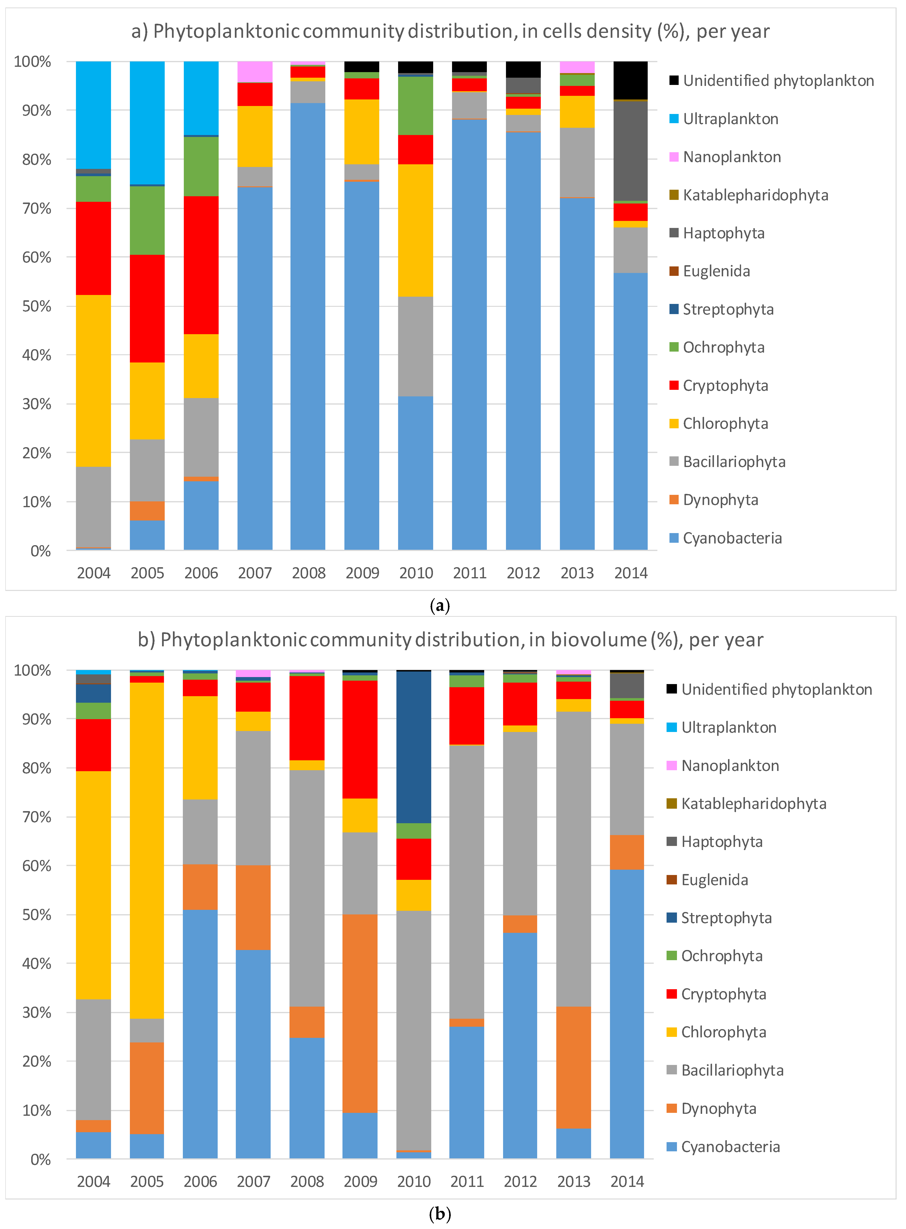
The aim of this study was to analyze the temporal patterns in cyanobacteria dominance in Lake Varese over a period of ten years (2004–2014) and to investigate the possibility to predict their abundance as a function of a set of meteorological data and water physical–chemical parameters. Overall, the picture of the phytoplankton community showed a change from 2006 with an increase of the cyanobacterial cells that accounted for more than the 50% of the total community, except in 2010. The community shift was also observed by the biovolume distribution, however, not so strongly dominated by the cyanobacteria particularly in 2008 and 2009 where the main contribution was due to the Bacillariophyta and Dynophyta, respectively as confirmed also by the other studies [50]. The different distribution in 2010 could be explained by a pilot study performed in 2009 to reduce the Phosphorus (P) loading by applying a lanthanum-modified bentonite clay to bind the P [32]. The authors showed a sharp reduction (more than 80%) of the P concentrations along the water column during 2009–2010 which may be the consequence of the dropped concentration of the cyanobacteria. However, the trend seems to be reverted with an increase of the cyanobacteria during the 2011–2014 years (Figure 2).

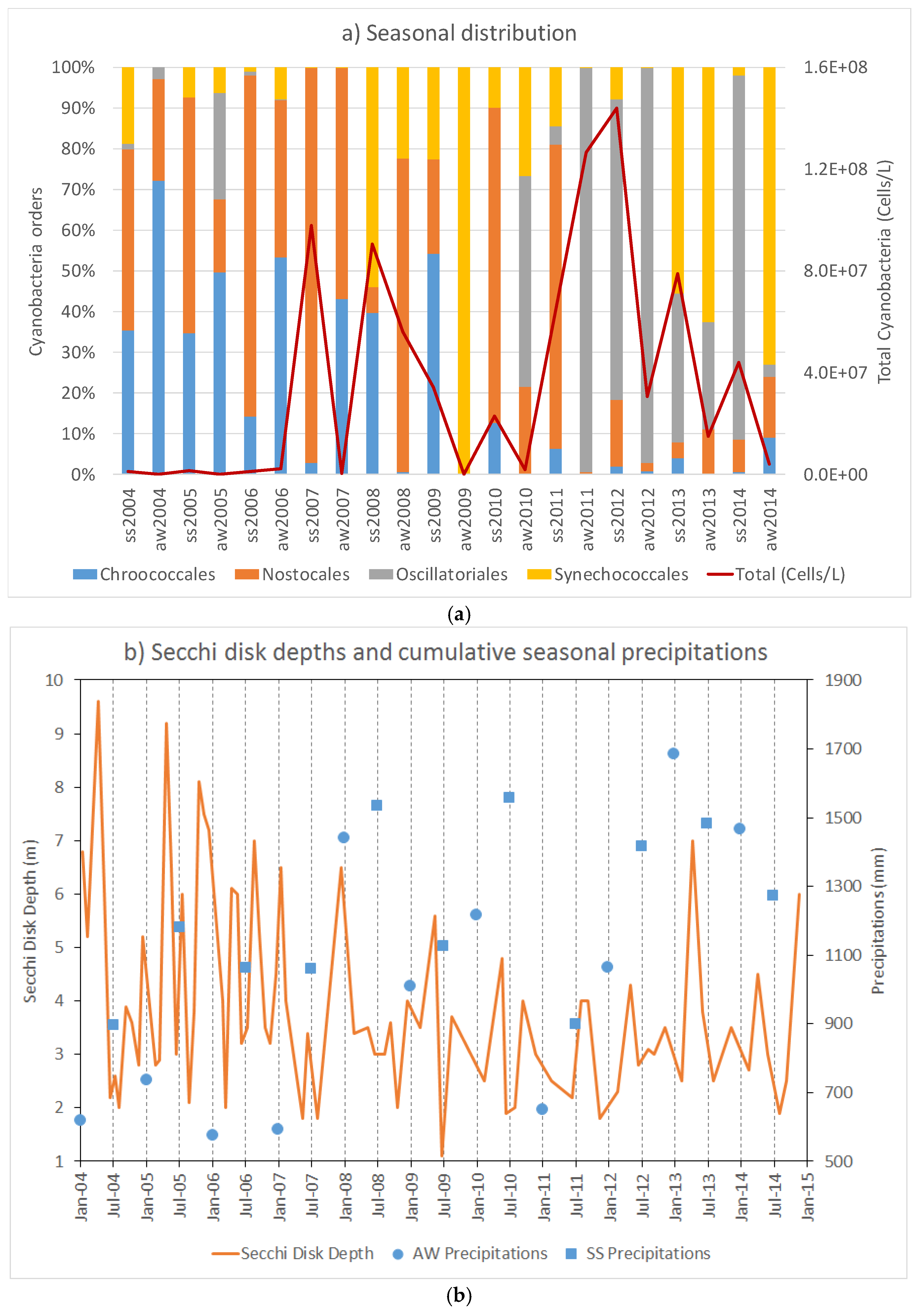
The cyanobacteria composition showed two distinct dominances; Chroococcales/Nostocales were mainly detected in the period from 2004 to 2009, while Oscillatoriales/Synechoccoccales increased after the 2010. In temperate regions, Oscillatoriales and most Chroococcales are associated with the increasing of temperature and water column stability; Nostocales, without the potential to fix nitrogen (Aphanizomenon), are associated with increasing TP concentration, while Synechoccoccales dominance is influenced by lower temperatures and water stability [4]. We could not have a clear picture of the dynamic distribution due to scarce periodicity of the sampling which would lead to a misinterpretation. After 2010, we observed an increase of the precipitation which may influence the shifting, however, Oscillatoriales have been reported to often dominate shallow polymictic eutrophic lakes showing cyclic successions between Microcystis (Chroococcales) and Planktothrix (Oscillatoriales). To get insight to the cyanobacterial biodiversity and spatio-temporal dynamic changes, it would need more frequent samplings such as weekly combined with the microscopy analysis and the metagenomics technique which allows a more deep analysis by sequencing the whole community (microbiome).

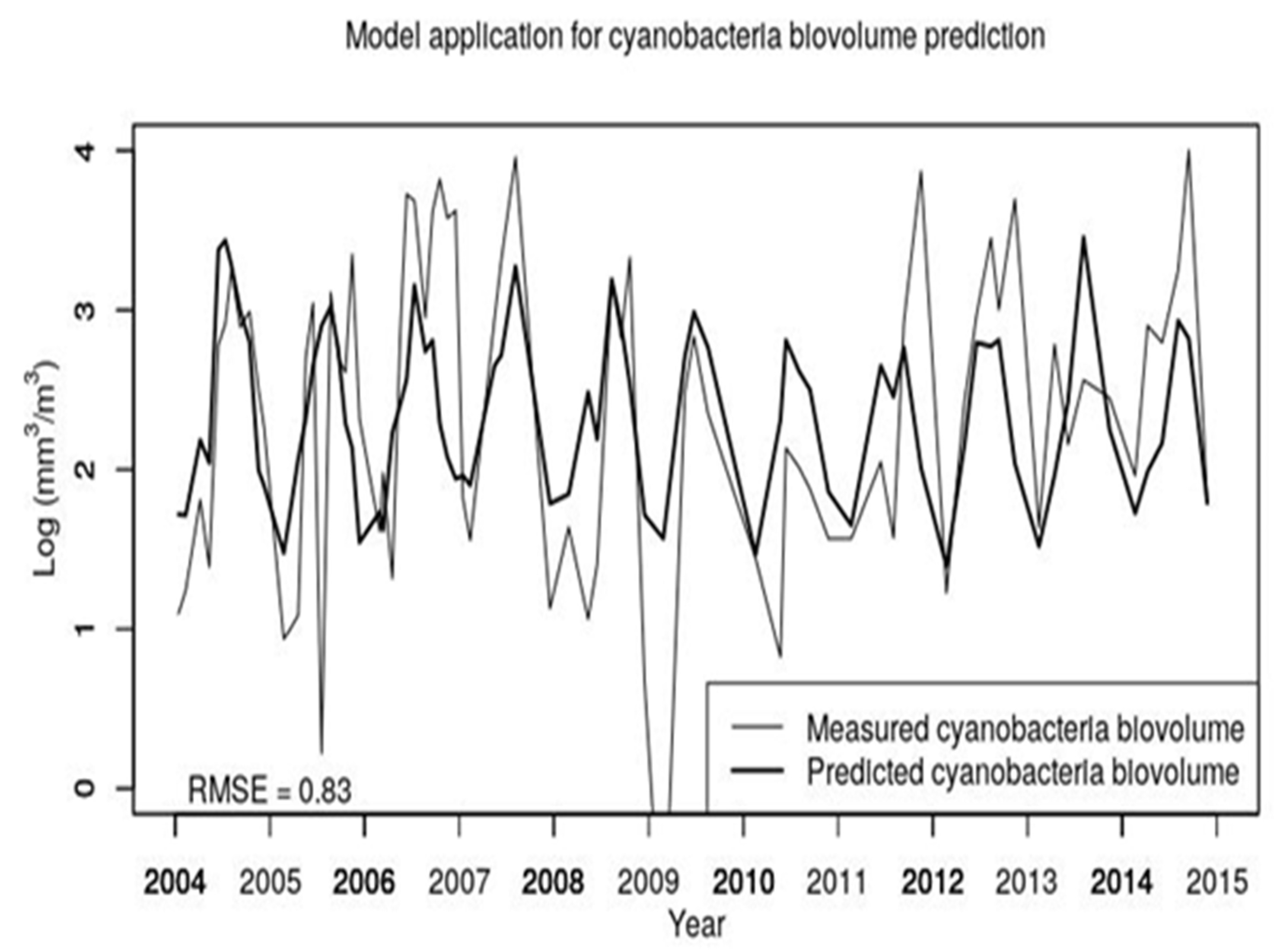
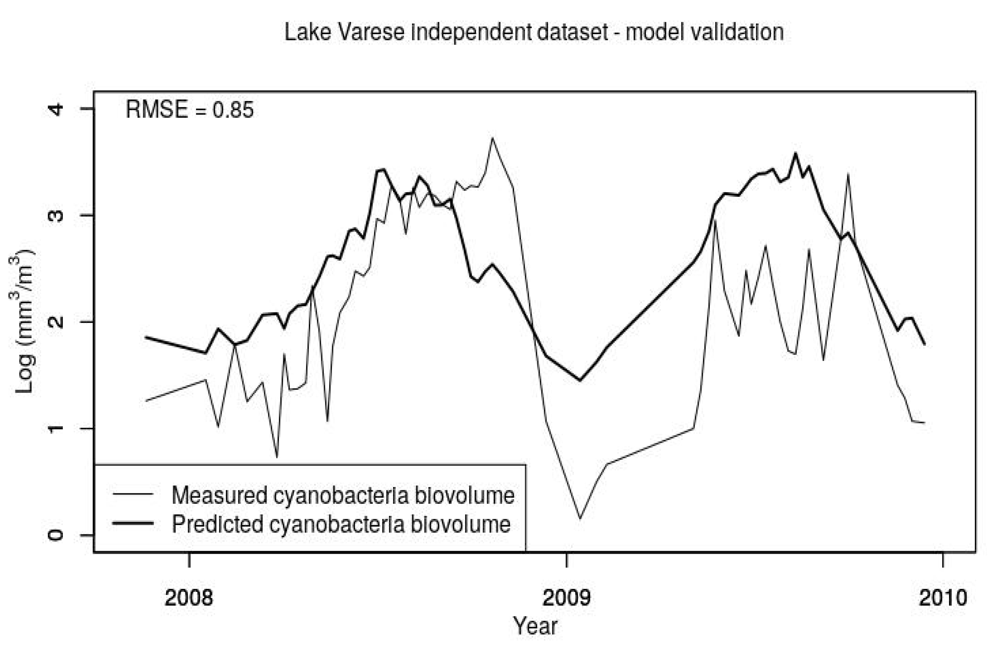
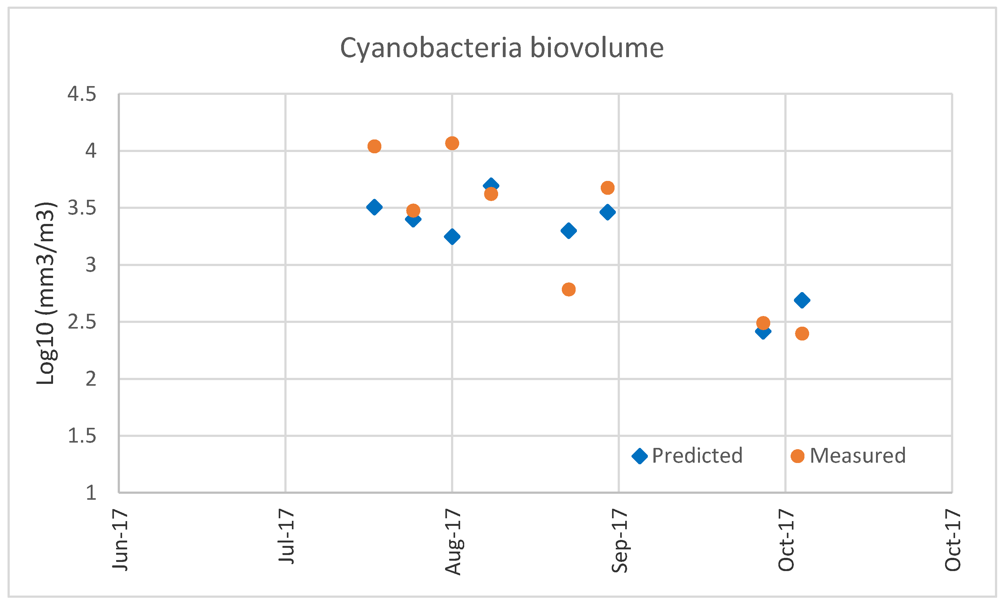
In the modeling studies, we did an attempt to develop an ANN using our data, but it resulted in an overfitted model while the selected MLR with just two predictors suggests that a general relationship has been captured as also confirmed by the validation step (see Figure 6), further supporting the robustness of the model as an accepted predictor. In our studies, we did not use the cell density as parameter (although available for the data set as shown in Figure 2) because the cell size can vary considerably within and between species, and toxin concentration relates more closely to the amount of dry matter in a sample than to the number of cells. In addition, cell identification by optical microscopy may underestimate the real value of cyanobacteria cells, indeed, smaller species may be (classified) reported as ultraplankton [51]. Therefore, the biovolume was selected as a more appropriate parameter. Furthermore, the biovolume measurements require less time for the microscopic analysis than cell identification and enumeration providing data with lower uncertainties. The parameters selected in this work such as the water temperature, DO, nutrient availability, and the water transparency measured as SD, play a key role in the occurrence of cyanobacterial blooms [19,20,22,23,26,27,52,53,54]. In addition to these factors known to be good predictors for cyanobacteria abundance, we tried to evaluate whether the air temperature could be considered as parameter. Indeed, air temperature is one of the main factors driving the evolution of water temperature in a lake [55] and influencing as well the vertical temperature profile and lake stratification [56], which are both important parameters for the occurrence of algal bloom outbreaks. In Lake Varese and generally in monomictic lakes, during spring, when air temperature rises, water stratification normally starts to build-up, stabilizes during summer until fall, when decreasing air temperatures break the stratification. Another factor which may lead to changes in water turbulence is the wind stress.

Taranu et al. has shown conflicting results on the response of cyanobacteria to climate and nutrients for dimictic (lakes that mix from top to bottom in two water mixing periods within a year) and polymictic lakes (mix from top to bottom for more than two water mixing periods) [23]. In dimictic lakes the stronger predictor was water-column stability, while for polymictic lakes, was nutrients loading. Journey et al., focusing on two monomictic lakes (mix from top to bottom during one mixing period per year), found strong correlations between cyanobacterial biovolumes and water stratification, while an opposite relationship was found with the nutrient levels [29]. 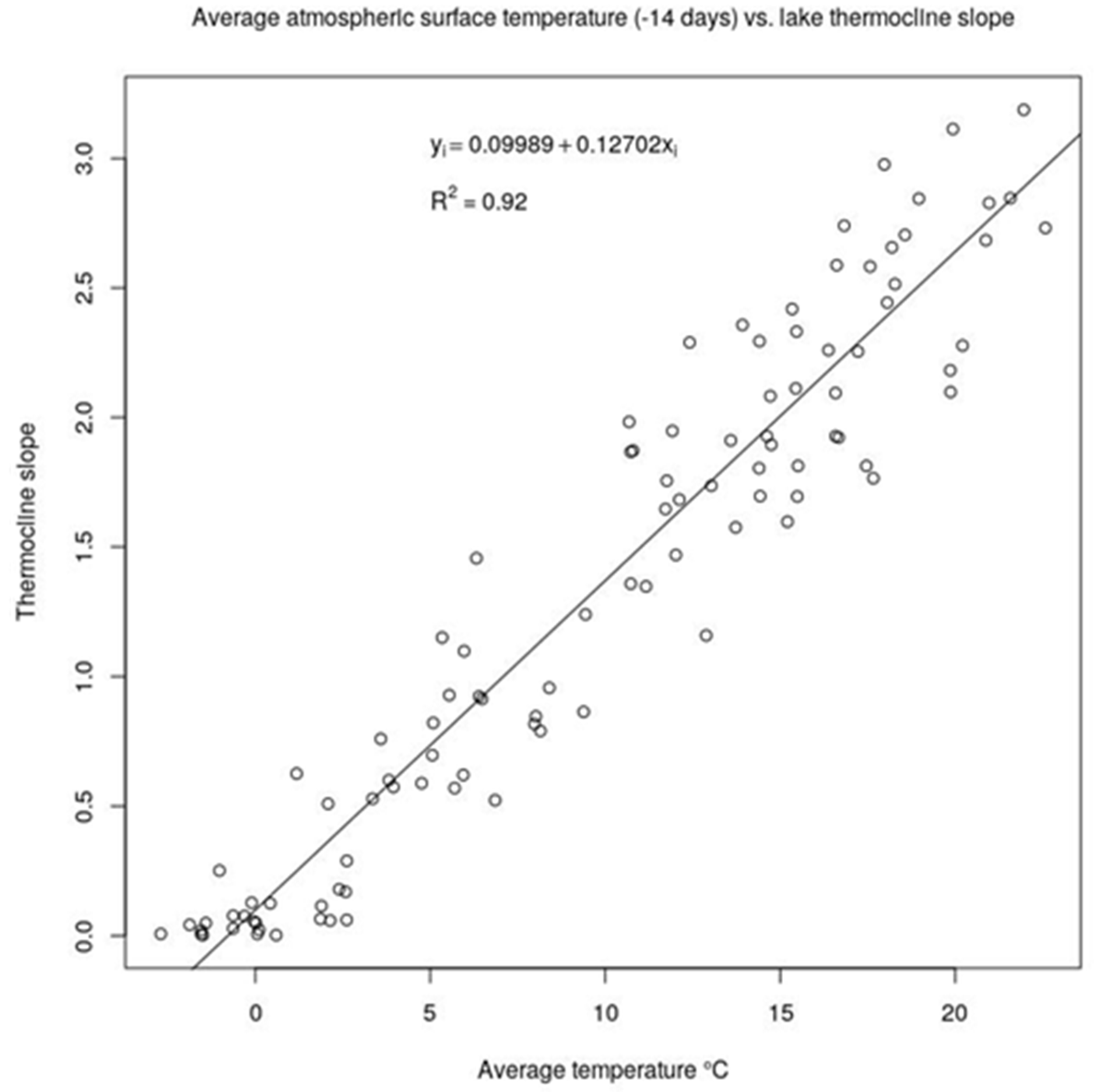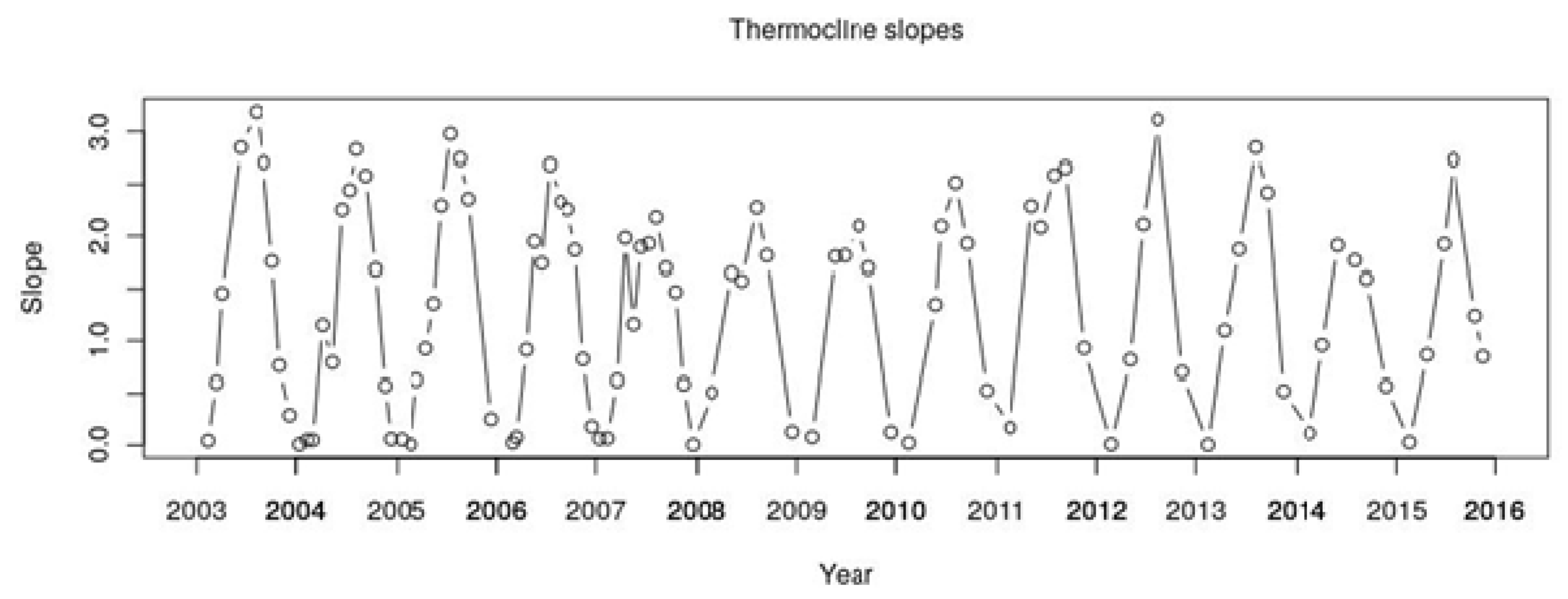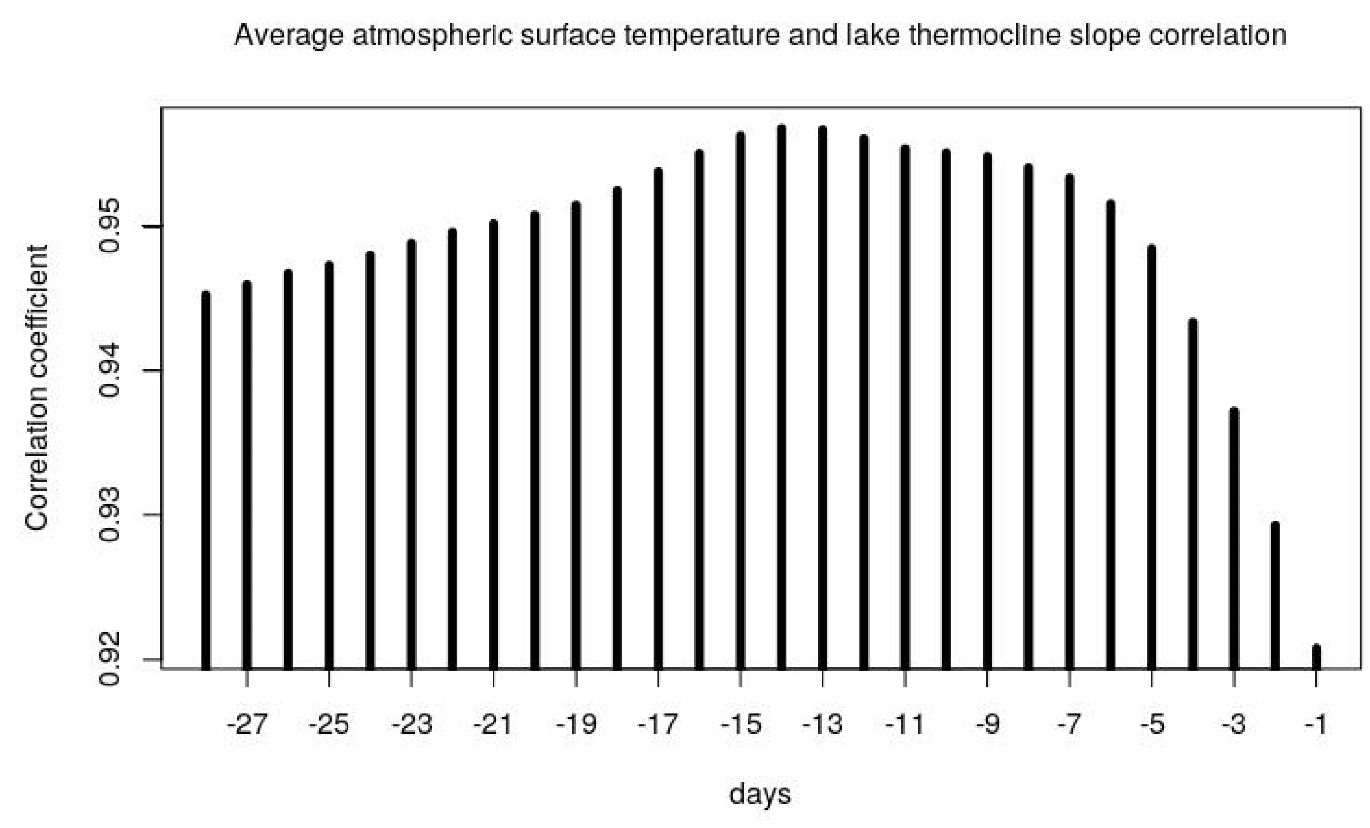In addition, it has been shown that the meteorological variables as air temperature, wind speed, and relative humidity, could be drivers of hypolimnetic anoxia, which is an indirect consequence of thermal stratification [28]. Indeed, temperature and stratification are cross-linked factors, with stratification forming and strengthening at higher air and water temperatures. In this paper, based on this correlation, we have demonstrated that 14-days average air temperature can be used as a proxy of the stratification strength for Lake Varese (Figure A3 in Appendix A and Figure 4). Indeed, the strongest correlation was found at 14 days (T14) preceding the current water temperature and the parameter T14. Despite wind speed being generally a physical variable influencing lake stratification [57], the lack of relationship with the thermocline slopes can be explained because the Lake Varese area usually does not experience strong wind speed. Based on that and considering that phosphorous is one of the most important factors for lake management [17], the model using T14 and total phosphorous (TP, model No.2 in Table 3) was chosen in this work as the best candidate to predict the Cyanobacteria biovolume at Lake Varese. In our analysis, the model using ammonium nitrogen (AN) as predictor (model No.5 in Table 3) was not considered further because AN is only one form of available nitrogen in water while it is known that all bioavailable forms of nitrogen (ammonium nitrogen, nitrate nitrogen, urea, and alanine nitrogen) influence the cyanobacteria abundance [58].

Nevertheless, the predictive power of this model is rather low, representing only about 30% of the total variability. The difficulty of predicting cyanobacteria blooms using physico–chemical environmental variables is a common problem highlighted also by previous studies [17,23,59]. On the other hand, as reported by Janssen et al., it is urgent and challenging to provide an algal bloom prediction at global level for the lakes [21]. The 14-days average air temperature together with total phosphorus can be, therefore, used to predict an algal outbreak two weeks in advance and, eventually, to adopt management actions to reduce their occurrence in monomictic and eutrophic shallow lakes.

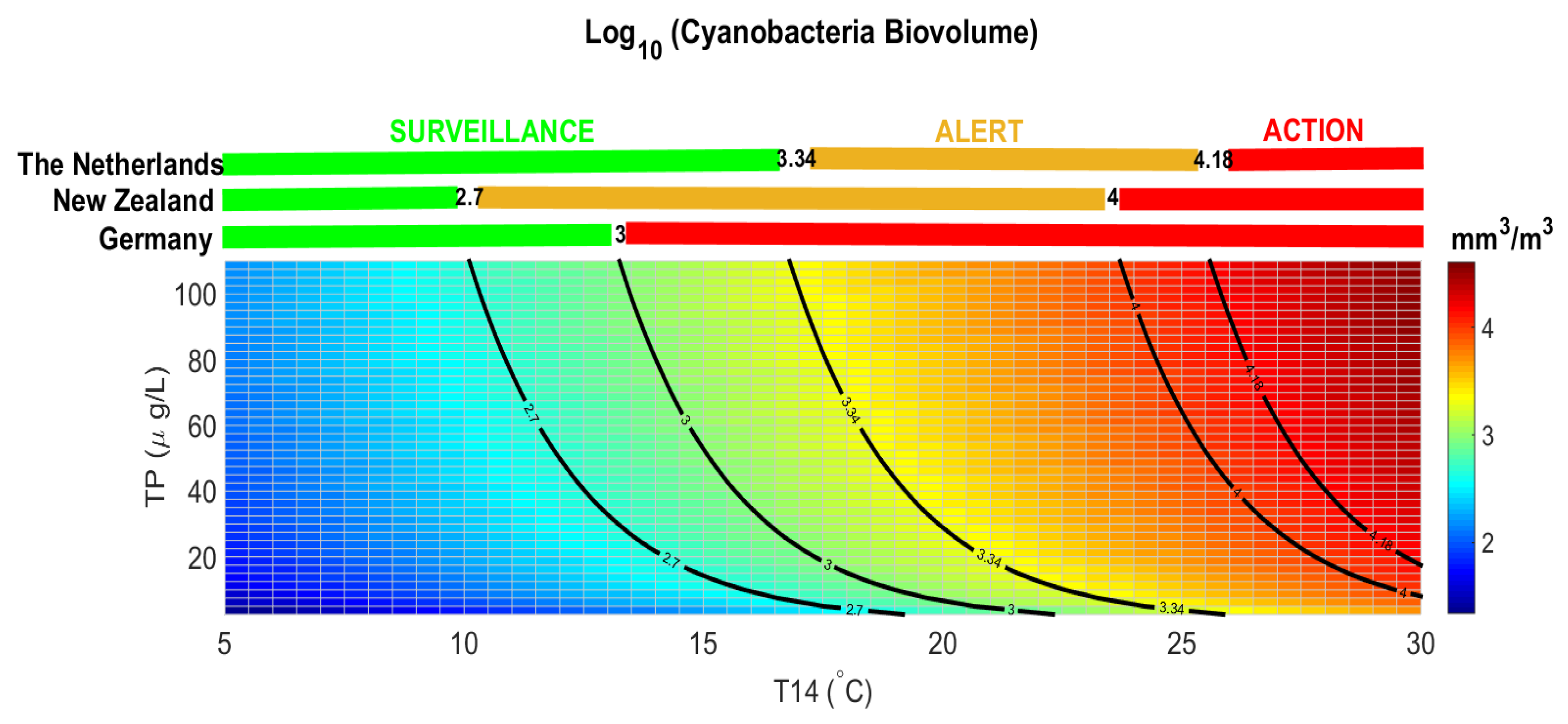
The threshold for health alert in recreational waters is normally defined for cyanobacterial density in many countries. A density of 100,000 cyanobacterial cells per ml (which is equivalent to approximately 50 µg/L of chlorophyll-a if cyanobacteria dominate) is a guideline for a moderate health alert in recreational waters [60], although the regulated threshold varies at national level. The conversion of cyanobacteria cell density into biovolume is not simple, as measurements of the cyanobacteria genera/species are needed [41]. Each country is free to define the alert values for the presence of cyanobacteria either in cell abundance or in biovolume [61], only few countries defined thresholds in terms of cyanobacterial biovolume (Figure 7). The Netherlands and New Zealand defined a surveillance level for cyanobacetria biovolume below 2.5 mm³/L (LOG CyanoBV = 3.34 mm³/m³) and 0.5 mm³/L (LOG CyanoBV = 2.7 mm³/m³), respectively. An alert is set above these thresholds requiring weekly monitoring and issue warning to the public. Above 15 mm³/L (LOG CyanoBV = 4.18 mm³/m³) and 10 mm³/L (LOG CyanoBV = 4 mm³/m³) The Netherlands and New Zealand authorities set an action level, continue the monitoring, notify the public of a potential risk to health, and if potentially toxic taxa are present, consider testing samples for cyanotoxins. Germany defined a single threshold for surveillance and alert level at 1 mm³/L (LOG CyanoBV = 3 mm³/m³), above which local authorities must publish warnings, discourage bathing, and consider temporary closure.

5. Conclusions

The main findings of this study can be summarized in the following points:

• In Lake Varese, a shift in the phytoplankton community distribution towards cyanobacteria dominance onwards 2010 was observed;
• This change may be related to changes in the nutrients, as well as precipitation patterns, as suggested by other studies, but more frequent samplings combined with the microscopy analysis and the metagenomics technique (microbiome) would allow a more conclusive analysis;
• Air temperature can be used as a good proxy of the lake surface water temperature and of the lake stratification;
• The 14 days mean air temperature showed the highest correlation with lake stratification strength derived by vertical water temperature profiles. At surface, this parameter is easily computable from weather forecast data, and together with total phosphorus continuous measured in situ, can be used as an early warning tool to anticipate by two weeks the beginning of cyanobacteria blooms in Lake Varese.

This model can help predict and mitigate the impact of climate change on water and ecosystem resource management.

References

1. Whitton, B.A.; Potts, M.E. The Ecology of Cyanobacteria; Springer: Dordrecht, The Netherlands, 2000. [Google Scholar]
2. Ho, J.C.; Michalak, A.M.; Pahlevan, N. Widespread global increase in intense lake phytoplankton blooms since the 1980s. Nature 2019, 574, 667–670. [Google Scholar] [CrossRef]
3. Sanseverino, I.; Antonio, D.C.; Pozzoli, L.; Dobricic, S.; Lettieri, T. Algal bloom and its economic impact. In JRC Technical Report; JRC: Ispra, Italy, 2016. [Google Scholar]
4. O’Neil, J.M.; Davis, T.W.; Burford, M.A.; Gobler, C.J. The rise of harmful cyanobacteria blooms: The potential roles of eutrophication and climate change. Harmful Algae 2012, 14, 313–334. [Google Scholar] [CrossRef]
5. Hudnell, H.K.; Dortch, Q. A Synopsis of Research Needs Identified at the Interagency, International Symposium on Cyanobacterial Harmful Algal Blooms (ISOC-HAB). In Cyanobacterial Harmful Algal Blooms: State of the Science and Research Needs; Hudnell, H.K., Ed.; Springer: New York, NY, USA, 2008; pp. 17–43. [Google Scholar]
6. Sivonen, K. Cyanobacterial toxins and toxin production. Phycologia 1996, 35, 12–24. [Google Scholar] [CrossRef]
7. Rastogi, R.P.; Madamwar, D.; Incharoensakdi, A. Bloom Dynamics of Cyanobacteria and Their Toxins: Environmental Health Impacts and Mitigation Strategies. Front. Microbiol. 2015, 6, 1254. [Google Scholar] [CrossRef] [PubMed] [Green Version]
8. Stauffer, B.A.; Bowers, H.A.; Buckley, E.; Davis, T.W.; Johengen, T.H.; Kudela, R.; McManus, M.A.; Purcell, H.; Smith, G.J.; Vander Woude, A.; et al. Considerations in Harmful Algal Bloom Research and Monitoring: Perspectives From a Consensus-Building Workshop and Technology Testing. Front. Mar. Sci. 2019, 6, 1–18. [Google Scholar] [CrossRef] [Green Version]
9. Beaulieu, M.; Pick, F.; Palmer, M.; Watson, S.; Winter, J.; Zurawell, R.; Gregory-Eaves, I. Comparing predictive cyanobacterial models from temperate regions. Can. J. Fish. Aquat. Sci. 2014, 71, 1830–1839. [Google Scholar] [CrossRef]
10. Ondenka, M. Correlations between several environmental factors affecting the bloom events of cyanobacteria in Liptovska Mara reservoir (Slovakia)—A simple regression model. Ecol. Model. Elsevier 2007, 209, 412–416. [Google Scholar] [CrossRef]
11. French, T.D.; Petticrew, E.L. Chlorophyll a seasonality in four shallow lakes (northern British Columbia, Canada) and the critical roles of internal phosphorous loading and temperature. Hydrobiologia 2007, 575, 285–299. [Google Scholar] [CrossRef]
12. Malek, S.; Syed Ahmad, S.M.; Singh, S.K.K.; Milow, P.; Salleh, A. Assessment of predictive models for chlorophyll-a concentration of a tropical lake. BMC Bioinform. 2011, 12, S12. [Google Scholar] [CrossRef] [Green Version]
13. Dimberg, P.H.; Olofsson, C.J. A comparison between regression models and genetic programming for predictions of chlorophyll-a concentrations in Northern Lakes. Environ. Model Assess. 2016, 21, 221–232. [Google Scholar] [CrossRef]
14. Malagó, A.; Bouraoui, F.; Grizzetti, B.; De Roo, A. Modelling nutrient fluxes into the Mediterranean Sea. J. Hydrol. Reg. Stud. 2019, 22, 100592. [Google Scholar]
15. Srivastava, A.; Ahn, C.Y.; Asthana, R.K.; Lee, H.G.; Oh, H.M. Status, Alert System, and Prediction of Cyanobacterial Bloom in South Korea. Biomed Res. Int. 2015, 2015, 8. [Google Scholar] [CrossRef] [PubMed] [Green Version]
16. Ghaffar, S.; Stevenson, R.J.; Khan, Z. Cyanobacteria Dominance in Lakes and Evaluation of Its Predictors: A Study of Southern Appalachians Ecoregion, USA. Matec Web Conf. 2016, 60, 02001. [Google Scholar] [CrossRef] [Green Version]
17. Downing, J.A.; Watson, S.B.; McCauley, E. Predicting Cyanobacteria dominance in lakes. Can. J. Fish. Aquat. Sci. 2001, 58, 1905–1908. [Google Scholar] [CrossRef]
18. Håkanson, L.; Bryhn, A.C.; Hytteborn, J.K. On the issue of limiting nutrient and predictions of cyanobacteria in aquatic systems. Sci. Total Environ. 2007, 379, 89–108. [Google Scholar] [CrossRef] [Green Version]
19. Beaulieu, M.; Pick, F.; Gregory-Eaves, I. Nutrients and water temperature are significant predictors of cyanobacterial biomass in a 1147 lakes data set. Limnol. Oceanogr. 2013, 58, 1736–1746. [Google Scholar] [CrossRef]
20. Huber, V.; Wagner, C.; Gerten, D.; Adrian, R. To bloom or not to bloom: Contrasting responses of cyanobacteria to recent heat waves explained by critical thresholds of abiotic drivers. Oecologia 2012, 169, 245–256. [Google Scholar] [CrossRef]
21. Janssen, A.B.G.; Janse, J.H.; Beusen, A.H.W.; Chang, M.; Harrison, J.A.; Huttunen, I.; Kong, X.; Rost, J.; Teurlincx, S.; Troost, T.A.; et al. How to model algal blooms in any lake on earth. Curr. Opin. Environ. Sustain. 2019, 36, 1–10. [Google Scholar] [CrossRef]
22. Kosten, S.; Huszar, V.L.M.; Bécares, E.; Costa, L.S.; Van Donk, E.; Hansson, L.A.; Jeppesen, E.; Kruk, C.; Lacerot, G.; Mazzeo, N.; et al. Warmer climates boost cyanobacterial dominance in shallow lakes. Glob. Chang. Biol. 2012, 18, 118–126. [Google Scholar] [CrossRef]
23. Taranu, Z.E.; Zurawell, R.W.; Pick, F.; Gregory-Eaves, I. Predicting cyanobacterial dynamics in the face of global change: The importance of scale and environmental context. Glob. Chang. Biol. 2012, 18, 3477–3490. [Google Scholar] [CrossRef]
24. Wagner, C.; Adrian, R. Cyanobacteria dominance: Quantifying the effects of climate change. Limnol. Oceanogr. 2009, 54, 2460–2468. [Google Scholar] [CrossRef]
25. Wells, M.L.; Trainer, V.L.; Smayda, T.J.; Karlson, B.S.O.; Trick, C.G.; Kudela, R.M.; Ishikawa, A.; Bernard, S.; Wulff, A.; Anderson, D.M.; et al. Harmful algal blooms and climate change: Learning from the past and present to forecast the future. Harmful Algae 2015, 49, 68–93. [Google Scholar] [CrossRef] [PubMed] [Green Version]
26. JÖHnk, K.D.; Huisman, J.E.F.; Sharples, J.; Sommeijer, B.E.N.; Visser, P.M.; Stroom, J.M. Summer heatwaves promote blooms of harmful cyanobacteria. Glob. Chang. Biol. 2008, 14, 495–512. [Google Scholar] [CrossRef] [Green Version]
27. Walsby, A.E.; Hayes, P.K.; Boje, R.; Stal, L.J. The selective advantage of buoyancy provided by gas vesicles for planktonic cyanobacteria in the Baltic Sea. New Phytol. 1997, 136, 407–417. [Google Scholar] [CrossRef]
28. Snortheim, C.A.; Hanson, P.C.; McMahon, K.D.; Read, J.S.; Carey, C.C.; Dugan, H.A. Meteorological drivers of hypolimnetic anoxia in a eutrophic, north temperate lake. Ecol. Model. 2017, 343, 39–53. [Google Scholar] [CrossRef] [Green Version]
29. Journey, C.A.; Beaulieu, K.M.; Bradley, P.M. Environmental Factors that Influence Cyanobacteria and Geosmin Occurrence in Reservoirs. In Current Perspectives in Contaminant Hydrology and Water Resources Sustainability; Bradley, P.M., Ed.; InTech: Rijeka, Croatia, 2013; pp. 27–55. [Google Scholar]
30. Zaccara, S.; Canziani, A.; Roella, V.; Crosa, G. A northern Italian shallow lake as a case study for eutrophication control. Limnology 2007, 8, 155–160. [Google Scholar] [CrossRef]
31. Guilizzoni, P.; Lami, A.; Ruggiu, D.; Bonomi, G. Stratigraphy of specific algal and bacterial carotenoids in the sediments of Lake Varese (N. Italy). Hydrobiologia 1986, 143, 321–325. [Google Scholar] [CrossRef]
32. Crosa, G.; Yasseri, S.; Nowak, K.-E.; Canziani, A.; Roella, V.; Zaccara, S. Recovery of Lake Varese: Reducing trophic status through internal P load capping. Fundam. Appl. Limnol. Arch. Hydrobiol. 2013, 183, 49–61. [Google Scholar] [CrossRef]
33. Morabito, G.; Hamza, W.; Ruggiu, D. Carbon assimilation and phytoplankton growth rates across the trophic spectrum: An application of the chlorophyll labelling technique. J. Limnol. 2004, 63, 33–43. [Google Scholar] [CrossRef]
34. Ruggiu, D. Osservazioni conclusive. Considerazioni generali sull’evoluzione a lungo termine dei popolamenti planctonici. Fitoplancton. In C.N.R. Istituto Italiano di Idrobiologia, Ricerche sull’evoluzione del Lago Maggiore; Aspetti limnologici. Campagna 1992 e Rapporto quinquennale 1988–1992; Commissione Internazionale per la protezione delle acque italo-svizzere: Torino, Italy, 1993; pp. 115–116. [Google Scholar]
35. Mosello, R.; Panzani, P.; Pugnetti, A.; Ruggiu, D. An assessment of the hydrochemistry of the eutrophic Lake Varese (N. Italy), coincident with the implementation of the first restoration measures. Mem. Dell’istituto Ital. Idrobiol. 1991, 49, 99–116. [Google Scholar]
36. Premazzi, G.; Cardoso, A.C.; Rodari, E.; Austoni, M.; Chiaudani, G. Hypolimnetic withdrawal coupled with oxygenation as lake restoration measures: The successful case of Lake Varese (Italy). Limnetica 2005, 24, 123–132. [Google Scholar]
37. Ambrosetti, W.; Barbanti, L.; Sala, N. Residence time and physical processes in lakes. J. Limnol. 2003, 62, 1–15. [Google Scholar] [CrossRef] [Green Version]
38. Premazzi, G.; Dalmiglio, A.; Cardoso, A.C.; Chiaudani, G. Lake management in Italy: The implications of the Water Framework Directive. Lakes Reserv. 2003, 8, 41–59. [Google Scholar] [CrossRef]
39. Balzamo, S.; Martone, C. Metodi Biologici per le Acque Superficiali Interne; Manuali e Linee Guida 111/2014; ISPRA: Rome, Italy, 2014. [Google Scholar]
40. Utermöhl, H. Zur Vervollkommnung der quantitativen Phytoplankton-Methodik. Mitt. Int. Ver. Angew. Limnol. 1958, 9, 1–38. [Google Scholar] [CrossRef]
41. Sun, J.; Liu, D. Geometric models for calculating cell biovolume and surface area for phytoplankton. J. Plankton Res. 2003, 25, 1331–1346. [Google Scholar] [CrossRef] [Green Version]
42. Dee, D.P.; Uppala, S.M.; Simmons, A.J.; Berrisford, P.; Poli, P.; Kobayashi, S.; Andrae, U.; Balmaseda, M.A.; Balsamo, G.; Bauer, P.; et al. The ERA-Interim reanalysis: Configuration and performance of the data assimilation system. Q. J. R. Meteorol. Soc. 2011, 137, 553–597. [Google Scholar] [CrossRef]
43. Bresnan, E.; Davidson, K.; Edwards, M.; Fernand, L.; Gowen, R.; Hall, A.; Kennington, K.; McKinney, A.; Milligan, S.; Raine, R.; et al. Impacts of climate change on harmful algal blooms. MCCIP Science Review. 2013, 236–243. [Google Scholar] [CrossRef]
44. Paerl, H.W.; Paul, V.J. Climate change: Links to global expansion of harmful cyanobacteria. Water Res. 2012, 46, 1349–1363. [Google Scholar] [CrossRef]
45. Paerl, H.W.; Hall, N.S.; Calandrino, E.S. Controlling harmful cyanobacterial blooms in a world experiencing anthropogenic and climatic-induced change. Sci. Total Environ. 2011, 409, 1739–1745. [Google Scholar] [CrossRef]
46. Fiedler, P.C. Comparison of objective descriptions of the thermocline. Limnol. Oceanogr. 2010, 8, 313–325. [Google Scholar] [CrossRef]
47. Meriluoto, J.; Spoof, L.; Codd, G.A. Handbook of Cyanobacterial Monitoring and Cyanotoxin Analysis; Wiley: Chichester, UK, 2017. [Google Scholar]
48. Huisman, J.; Matthijs, H.; Visser, P. Harmful Cyanobacteria; Springer: Dordrecht, The Netherlands, 2005. [Google Scholar]
49. Nõges, P.; Nõges, T.; Ghiani, M.; Sena, F.; Fresner, R.; Friedl, M.; Mildner, J. Increased nutrient loading and rapid changes in phytoplankton expected with climate change in stratified South European lakes: Sensitivity of lakes with different trophic state and catchment properties. Hydrobiologia 2011, 667, 255–270. [Google Scholar] [CrossRef]
50. Nõges, P.; Nõges, T.; Ghiani, M.; Paracchini, B.; Grande, J.P.; Sena, F. Morphometry and trophic state modify the thermal response of lakes to meteorological forcing. Hydrobiologia 2011, 667, 241–254. [Google Scholar] [CrossRef]
51. Caron, D.A. Technique for enumeration of heterotrophic and phototrophic nanoplankton, using epifluorescence microscopy, and comparison with other procedures. Appl. Environ. Microbiol. 1983, 46, 491–498. [Google Scholar] [CrossRef] [PubMed] [Green Version]
52. Kimambo, O.N.; Gumbo, J.R.; Chikoore, H. The occurrence of cyanobacteria blooms in freshwater ecosystems and their link with hydro-meteorological and environmental variations in Tanzania. Heliyon 2019, 5, e01312. [Google Scholar] [CrossRef] [PubMed] [Green Version]
53. Takarina, N.D.; Wardhana, W. Relationship between cyanobacteria community and water quality parameters on intertidal zone of fish ponds, Blanakan, West Java. Aip Conf. Proc. 2017, 1862, 030114. [Google Scholar] [CrossRef]
54. Megard, R.O.; Settles, J.C.; Boyer, H.A.; Combs, W.S., Jr. Light, Secchi disks, and trophic states1. Limnol. Oceanogr. 1980, 25, 373–377. [Google Scholar] [CrossRef]
55. Piccolroaz, S.; Toffolon, M.; Majone, B. A simple lumped model to convert air temperature into surface water temperature in lakes. Hydrol. Earth Syst. Sci. 2013, 17, 3323–3338. [Google Scholar] [CrossRef]
56. Hadley, K.R.; Paterson, A.M.; Stainsby, E.A.; Michelutti, N.; Yao, H.; Rusak, J.A.; Ingram, R.; McConnell, C.; Smol, J.P. Climate warming alters thermal stability but not stratification phenology in a small north-temperate lake. Hydrol. Process. 2014, 28, 6309–6319. [Google Scholar] [CrossRef]
57. Kerimoglu, O.; Rinke, K. Stratification dynamics in a shallow reservoir under different hydro-meteorological scenarios and operational strategies. Water Resour. Res. 2013, 49, 7518–7527. [Google Scholar] [CrossRef]
58. Chaffin, J.D.; Bridgeman, T.B. Organic and inorganic nitrogen utilization by nitrogen-stressed cyanobacteria during bloom conditions. J. Appl. Phycol. 2013, 26, 299–309. [Google Scholar] [CrossRef]
59. Oh, H.M.; Ahn, C.Y.; Lee, J.W.; Chon, T.S.; Choi, K.H.; Park, Y.S. Community patterning and identification of predominant factors in algal bloom in Daechung Reservoir (Korea) using artificial neural networks. Ecol. Model. 2007, 203, 109–118. [Google Scholar] [CrossRef]
60. Chorus, I.; Bartram, J. Toxic Cyanobacteria in Water: A Guide to Their Public Health Consequences, Monitoring and Management/edited by Ingrid Chorus and Jamie Bertram; World Health Organization: Geneva, Switzerland, 1999. [Google Scholar]
61. Chorus, I. Current Approaches to Cyanotoxin Risk Assessment, Risk Management and Regulations in Different Countries; Umweltbundesamt: Dessau-Roßlau, Germany, 2012. [Google Scholar]
Figure 1. Location of Lake Varese (red). The positions of the available meteorological stations in the region are indicated by the light blue dots (Regional Environmental Protection Agency Lombardia, ARPA), and the dark blue dot (the Joint Research Center). The red polygon in the lower right corner map indicates the location of the model grid-cell from the ERA-Interim atmospheric reanalysis, where Lake Varese is located.
Water 12 00675 g001
Figure 2. Distribution of the total phytoplankton community expressed in percentage (Y-axis) of the average of the annual campaign from 2004 to 2014. (a) On the top plot, the distribution is reported as percentage of cell density (cells/L); (b) on the bottom the distribution is shown as percentage of biovolume (mm3/m3). The total cell density and biovolume values for each year are reported in Table A1 in Appendix A.
Water 12 00675 g002
Figure 3. (a) The top graph shows a representation of total cyanobacteria community distribution as percentage, based on biovolume (mm3/m3). Community distribution is presented as the average of the annual campaigns data, grouped as Summer-Spring (ss) and Autumn-Winter (aw) seasons, and by order. The red line reports the total cyanobacteria number per data set; (b) bottom graph represents the Secchi disk depth (continuous line in orange) at each sampling campaign and the six-month cumulative precipitations, Autumn-Winter (aw, blue circles) and Spring-Summer (ss, blue squares).
Water 12 00675 g003
Figure 4. Relationship between the thermocline slopes and the average air temperature of current plus the preceding 14 days. Every dot is from a probe sampling campaign (from 2003 to 2015 included). The linear relationship is strong (R2 = 0.92) and without any relevant bias in the plot, thus supporting the use of the average air temperature of the current and the last 14 days as a proxy of water stratification.
Water 12 00675 g004
Figure 5. Measured and predicted cyanobacteria biovolumes at Lake Varese for all samples collected during the period 2004–2014. Predicted values are calculated using model No.2 of Table 3. RMSE indicates the root mean square error of predicted vs. measured values.
Water 12 00675 g005
Figure 6. Validation of the model: Measured and predicted cyanobacteria biovolumes at Lake Varese using an independent dataset (not included in the MLR analysis) of water samples collected at Lake Varese during the period 2008–2010 by JRC. RMSE indicates the root mean square error of predicted vs. measured values.
Water 12 00675 g006
Figure 7. Estimated cyanobacteria biovolume calculated for Lake Varese using model No.2 of Table 3. The colored field represents LOG CyanoBV at different levels of the two predictors, T14 ranging between 5 and 30 °C, and TP ranging between 2.5 and 110 μg/L. The colored bars above the plot and the black lines refers to examples of threshold levels for cyanobacteria biovolume (surveillance in green, alert in orange, and action in red) of defined by legislation in The Netherlands, New Zealand, and Germany.
Water 12 00675 g007