A Front-Line and Cost-Effective Model for the Assessment of Service Life of Network Pipes

Abstract

In any water utility, a reliable assessment of the service life of the network pipes is a key piece within the big puzzle of assets management. This paper presents a new statistical model (basic pipes life assessment, BPLA) to assess the service life of pipes, to locate the pipes on the failures bath curve and to forecast the expected failures in future years. Its main novelties are the processing of pipe information (is that information what is adapted to the classical maintenance engineering and not the other way back) and the definition of two different time variables that can be analyzed in parallel. The first novelty makes the model less demanding in terms of data and software tools than others currently available, and the second one allows to get all the results after one single stage of calculation. To show its usability, the BPLA has been applied to a pipe network that supplies water to 500,000 citizens for which two years of failure records are available. Procedures and results have been compared to the well-known Weibull proportional hazard model (WPHM), with final relative errors lower than 10% and 15% on each particular result.

1. Introduction

If asset management is a key area in any urban water utility, an accurate knowledge of the pipes service life is a key aspect within asset management. There are many advantages to knowing the current condition of pipes and their remaining life until renovation. From a technical perspective, hydraulic operation and maintenance policies may be optimized; from an economic perspective, network expenditures and costs may be kept at minimum levels, and from a social perspective, the subsequent level of service may be maintained as high as possible.

One main reference in determining the optimal replacement time of pipes dates back from 1979 by Shamir and Howard [1]. It consisted of a deterministic model for the economic optimization of repair vs. renovation times. Since then, the study of pipe performance and resulting lifetime has adopted different approaches—not only deterministic, but also statistical and probabilistic. A good general approach to networks maintenance with an insight on failure forecasting was presented by Lauer [2]. Rostum [3] provided a comprehensive statistical analysis of the pipe failure process based on a non-homogeneous Poisson process. The influence of economies of scale was added to a pipe renewal model by Kleiner et al. [4] and Fuchs-Hanusch et al. [5] proposed a correction on the pipes life-cycle equation by including leak detection costs growing with pipes age. A failure model based on an exponential-Weibull distribution was developed by Scholten et al. [6]; additionally, it was used in a multi-criteria decision analysis to grade potential rehabilitation strategies in the long term. Amaitik et al. and others [7,8,9] proposed the use of neural networks for failure prediction and pipe renovation, while Kabir [10] targeted the same goal by using a Bayesian framework. More recently, other approaches have been explored: Martinez [11] focused on the cause of failures through explanatory variables by means of a Bayesian analysis, Motiee et al. [12] compared four different regression models, Di Nardo et al. [13] applied fractal theory to assess the resilience of pipe failures, and Kutylowska [14] predicted pipe failure rates through support vector machines.

In particular, the research on the Weibull proportional hazard model (WPHM), which is the bench test for the model presented in this paper, can be followed through the works by Le Gat and Eisenbeis and others [15,16,17,18,19].

From another perspective, other works have combined different but complementary approaches. The interrelations between statistical and physical models were explored by Davis et al. and others [20,21,22], Yoo et al. [23] prioritized rehabilitation by adding normal and emergency operation conditions, while D’Ercole et al. [24] connected it with reliability-approach models.

Over all these years and varieties of studies and approaches, several works [3,25,26,27] have made successive organized classifications of the state of the art, at each moment, in this field of research.

In parallel with scientific research, several software packages have been developed [28,29,30,31], either produced by large corporations on utilities management, engineering consultancy companies or other organizations. Some of them are currently available in the market.

In spite of this wide context, according to the authors’ experience, small- and medium-sized water utilities still face significant barriers when they try to incorporate these kind of methodologies to their own asset management policies. It is due, in general terms, to an imbalance between the requirements needed and their limited resources available. The latest models published in scientific journals are not in a form that can be directly implementable in practice for a water utility, as scientific skills and knowledge, as well as specialized software, are often essential for these models. On the other hand, commercial software, apart from the cost itself, might have undesired implications for the utility in terms of outsourcing, unknowns on the process behind the results, sensible data, etc. Above the particular issues of one or another alternative, the fact is that the latest models rely on a large and varied amount of historical data that is not usually available (or reliably available) in the case of many small- and medium-sized water utilities.

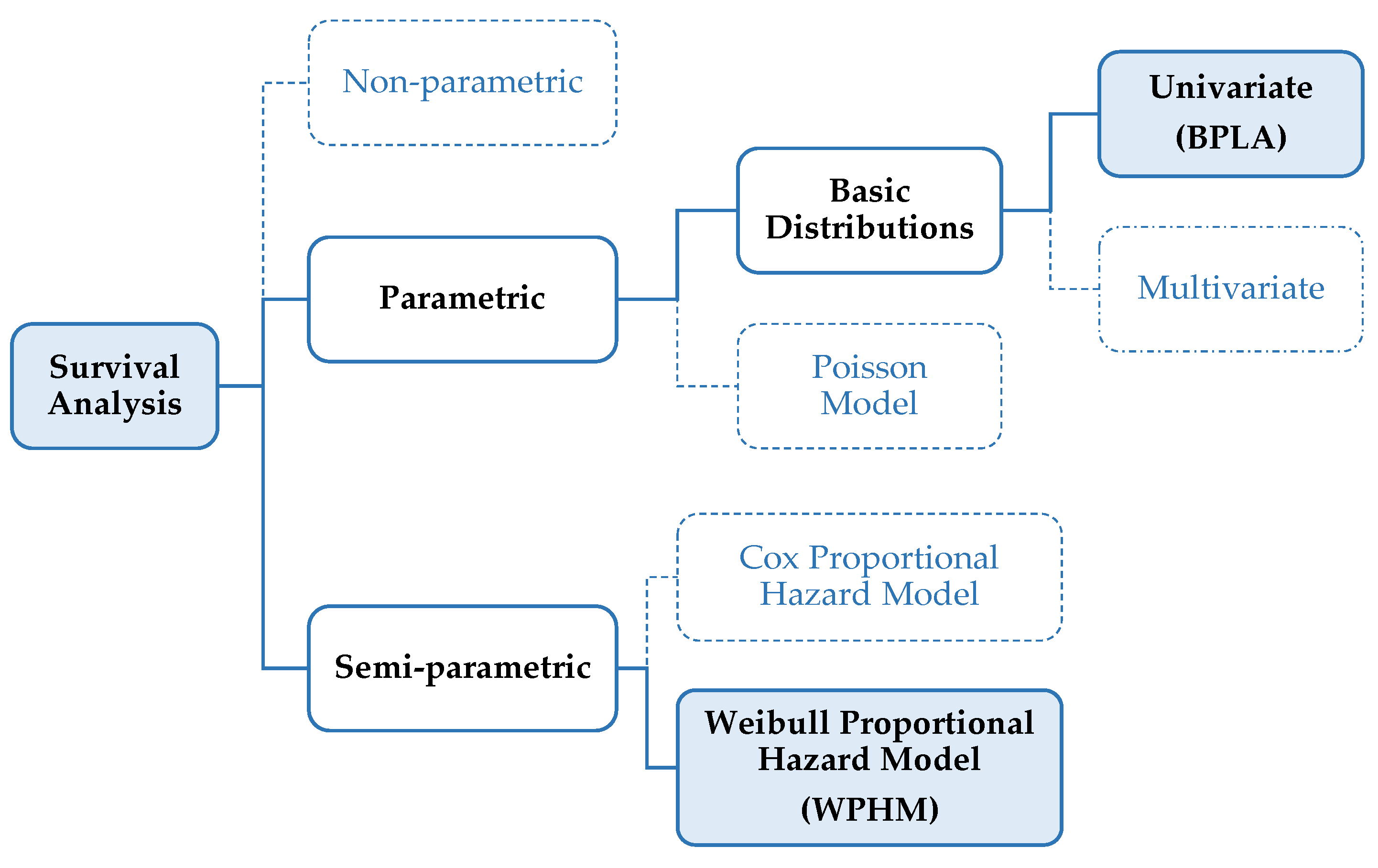
Aiming to overcome that barrier, this paper presents a new, simple statistic parametric univariate model (Figure 1), named basic pipes life assessment (BPLA). It is an application of concepts coming from the industrial maintenance engineering [32,33] (for non-repairable components) to the particular case of network pipes (repairable components). Its first novelty is that instead of adapting the industrial maintenance theory to the network pipes, the BPLA makes the adaptation the other way, i.e., the characteristics of pipes are modified (segmentation) to fit the requirements of the components of the industrial maintenance theory they work with. The second novelty is that for each failure date, two different time variables are defined ($\mathrm{LtF}$ and $\mathrm{TtF}$). This way, though there is only one type of analysis to be performed, it can be applied in parallel to both variables and all the results are obtained after only one calculation stage.

The outcome is a model less demanding than the ones referenced above in terms of:

• Required data, which are only the pipe failure records, as well as the basic pipe characteristics (material, length and diameter). Therefore, the model attention is only focused on the failure times, not on potential causes, influential factors, costs or physical models.
• Complexity of analysis, which is reduced to statistical fittings to usual distributions, mainly Weibull, but normal, log-normal, etc., can be also used.

The results obtained for each group of pipes analyzed through BPLA are three: (i) an estimation of the average service life, (ii) the location of the pipe group on the bath curve [32] according the time evolution of its failures and (iii) a forecast of the future expected failures in the next years. The final advantage of the model proposed is the cost-effectiveness of its application. As it will be shown below, notwithstanding this main focus on a direct, practical applicability, the quality level of results produced is equivalent to that from other related and more complex model on the same data sets. As a conclusion, those are the gaps that BPLA intends to cover either from the literature and the engineering sides.

In order to show the applicability of the BPLA, it has been implemented on a water utility that services 500,000 people with two years of available (and reliable) pipe failure records. This is a rather limited amount of data for this kind of studies. Yet, such scarcity is not unusual in many small- to medium-sized utilities and, at the same time, it has not prevented the sought-after results. The implications of this restriction are developed in the Discussion section.

In order to show the consistency of the results obtained, the WPHM has subsequently been applied to the same data. The WPHM is a well-known [15,16,17,18,19] semi-parametric model (Figure 1) that implies a significant complexity compared to the BPLA.

The next section of the paper Materials and Methods describes the foundations, equations, parameters and results of the BPLA. In addition, a quick summary of the WPHM is included. Particular attention has been focused on data processing and other practical aspects in order to ease follow-up by the interested reader. The following section, Case Study and Results shows the case study analyzed, the information initially available, the statistical fittings performed, and the results obtained by both BPLA and WPHM, as well as the interpretation for each one. In the Discussion section, a double comparison is made. First, the results obtained are quantitatively analyzed. Then, the practical advantages are graphically summarized. Finally, the Conclusions section remarks the contributions presented in the paper and the interest of this method, particularly, for water utilities at their initial stages in this area of asset management.

2. Materials and Methods

Obviously, pipes are not bulbs. A bulb is the classical example of a non-repairable element. It works until it fails and then, it must be replaced for a new bulb. Conversely, a pipe can be considered as a repairable element, because it can be repaired after the first failure, and again every time, after a new failure happens. From the pipe installation moment, its service life keeps increasing, no matter the repairs undertaken, until it is finally replaced. Such replacement will probably have a direct relationship to the number of repairs occurred, although this does not necessarily have to be always the case. In maintenance engineering, the analysis of the service life of non-repairable elements, like bulbs, can be posed in simpler terms than that for repairable elements, like mechanical machines or electronic devices [32,33]. The complexity of the current statistical models for pipe failure analysis [3,10,17,34] confirm this fact. However, a pipe is essentially different from a complex machine—though being repairable as a whole, a pipe could be considered as a non-repairable element if only the length of the pipe intervened in the reparation (or partial replacement) is focused on. Through an assumable simplification, that short length of the pipe has reached the end of its service life. This way, by taking advantage of dividing, virtually, each pipe into short segments, which could be individually analyzed, the basics of statistical analysis of non-repairable elements may be applied to pipe networks. These are the fundamentals of the BPLA model.

2.1. Development and Application of the BPLA

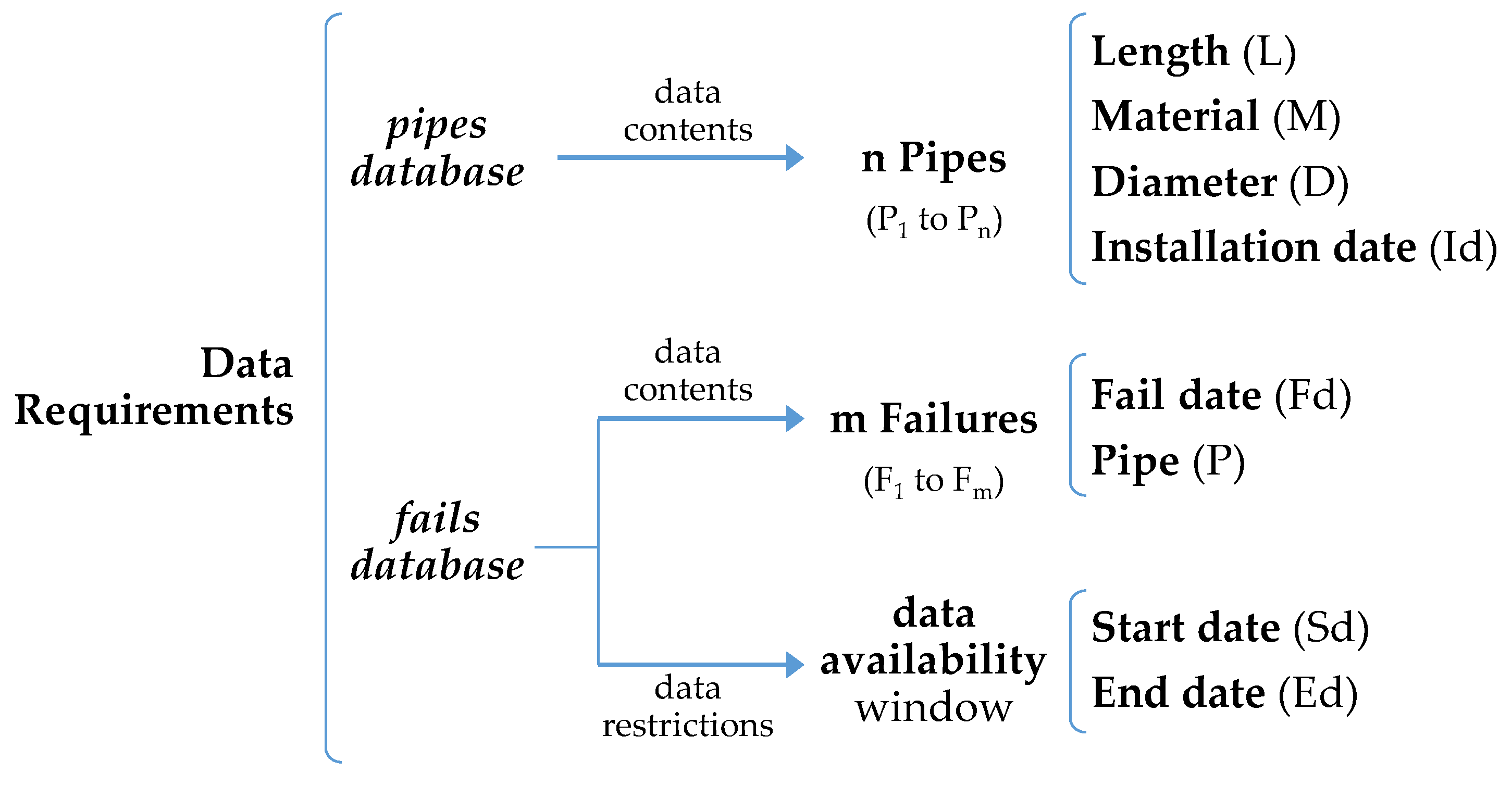
Data requirements and organization: The information needed for the BPLA comes from two different sections of the infrastructure database: pipes and failure records (Figure 2). For the pipes, the only needed characteristics are the length, diameter, material, and installation date, although other kind of information might be also welcome; for example, the DMA, which might help later to select the groups of pipes.

This information may be organized in the so-called pipes table as shown in

Table 1. Structure of the pipes table.

Pipe	Instal. Date	Length	Diameter	Material
P1	Id1	L1	D1	M1
…	…	...	...	...
Pi	Idi	Li	Di	Mi
Pj	Idj	Lj	Dj	Mj
…	…	...	...	...
Pn	Idn	Ln	Dn	Mn

—n being the total number of pipes, the pipes table will be compounded by n rows. For clarity purposes, four pipes (1, i, j and n) will be used in this paper to follow the development of the model.

As to the failures information, the basic data needed are the date and pipe for each failure occurrence. Additionally, the position, in a temporal order, of all the failures occurred in the same pipe must be also considered. That information may be structured in the fails table (

Table 2. Structure of the fails table.

Failure	Fail Date	Pipe	Fail Order in Pipe
F1	Fd1	Pi	Pi_O1
F2	Fd2	Pj	Pj_O1
F3	Fd3	Pn	Pn_O1
F4	Fd4	Pj	Pj_O2
F5	Fd5	Pj	Pj_O3
…	...	…	...
Fm	Fdm	Pn	Pn_O2

), where m is the total number of failures.

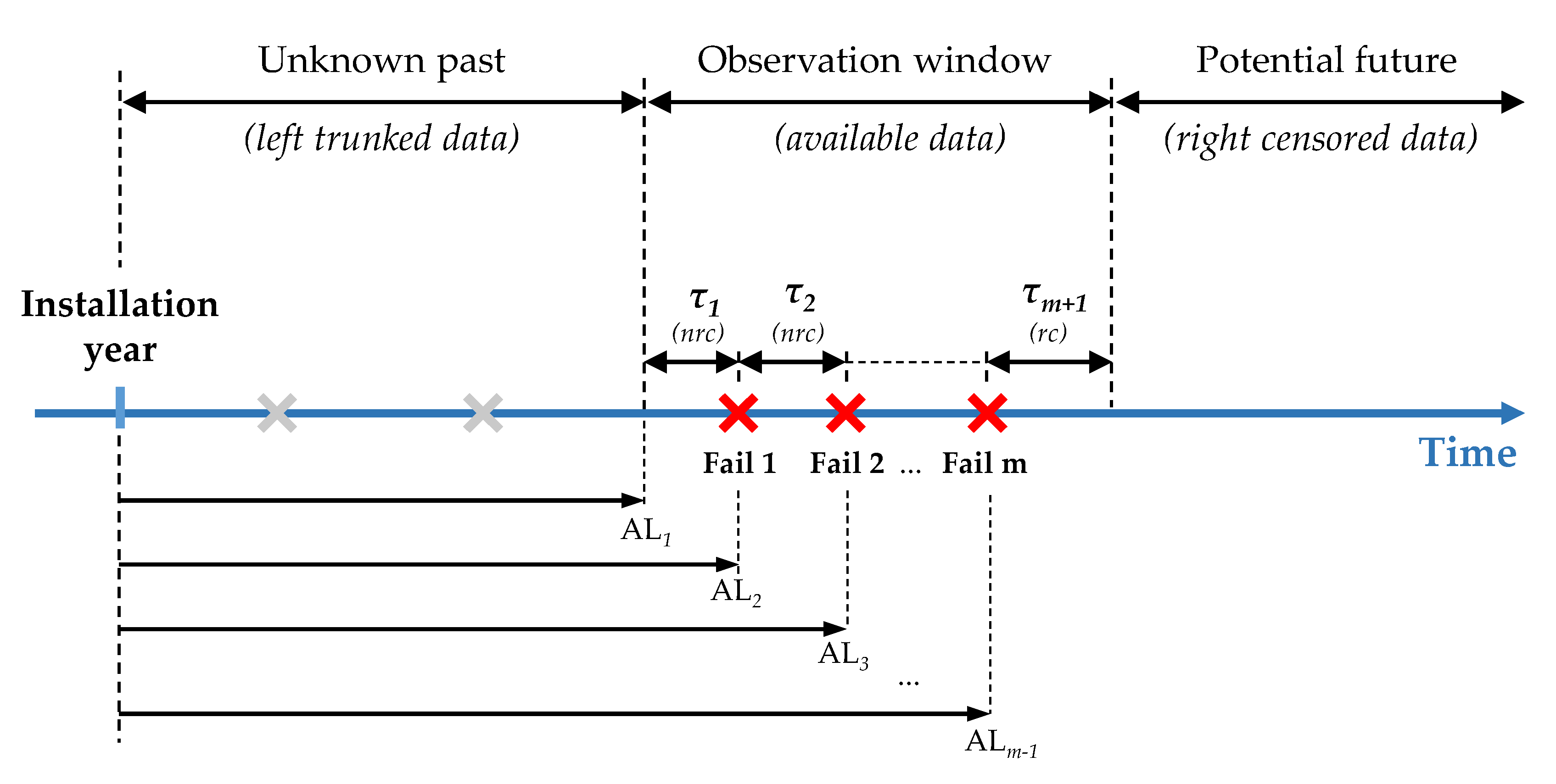
In many cases, the way the failure information was recorded in the past by many water utilities was not as accurate as required by this kind of analysis. This means that it is not unusual to find large gaps of accurate information from the time the pipes were installed. Because of this inequity on the available failure data, it is essential to find the widest possible window of failure data, in which all the network pipes are included. These start date and end date (Sd and Ed) of the availability window, which are not data information but data restrictions instead, will be key for the time variables of the model.

Once that window is identified, all the failures within are the ones to be displayed in the fails table. Unavoidably, the knowledge of failure data is (left) trunked for dates before the window’s start—failures might have occurred or not, but it is an unknown past. Furthermore, the failure data is (right) censored for dates after the window’s end—pipes are in operation in that moment, but they might fail later, which is the potential future [35].

The common renovation and maintenance operations in the network affect these two tables in two different ways. Repairs are considered as works that do not affect significantly the length of a pipe. In consequence, the pipe characteristics remain the same after a repair. This kind of intervention should be recorded as a failure occurrence and it will enlarge the fails table. Conversely, renovations are partial or total physical replacements of a pipe. After a renovation, there is a change in one or more components of the pipe database. In accordance, those changes will be reflected on the pipes table.

Pipe groups definition: The BPLA model works on the assumption that the groups of pipes to analyze are homogenous enough. Therefore, the first task consists of distributing all the network pipes into different groups according to their characteristics. As the case study will show, initial criteria rely on material, diameter ranges, or age ranges.

The most important condition is that each group of pipes must have at least 30 registered failures. This is imposed by the statistical fitting method that will be used later (maximum likelihood estimation) [36].

Data management: Once the pipe groups have been formed, the initial pipes table and fails table, must be divided into as many pipe and fail tables as there are pipe groups—one pipes table and one fails table containing the information of (only) the pipes that are gathered in each pipe group. Calculations will be individually applied to each group.

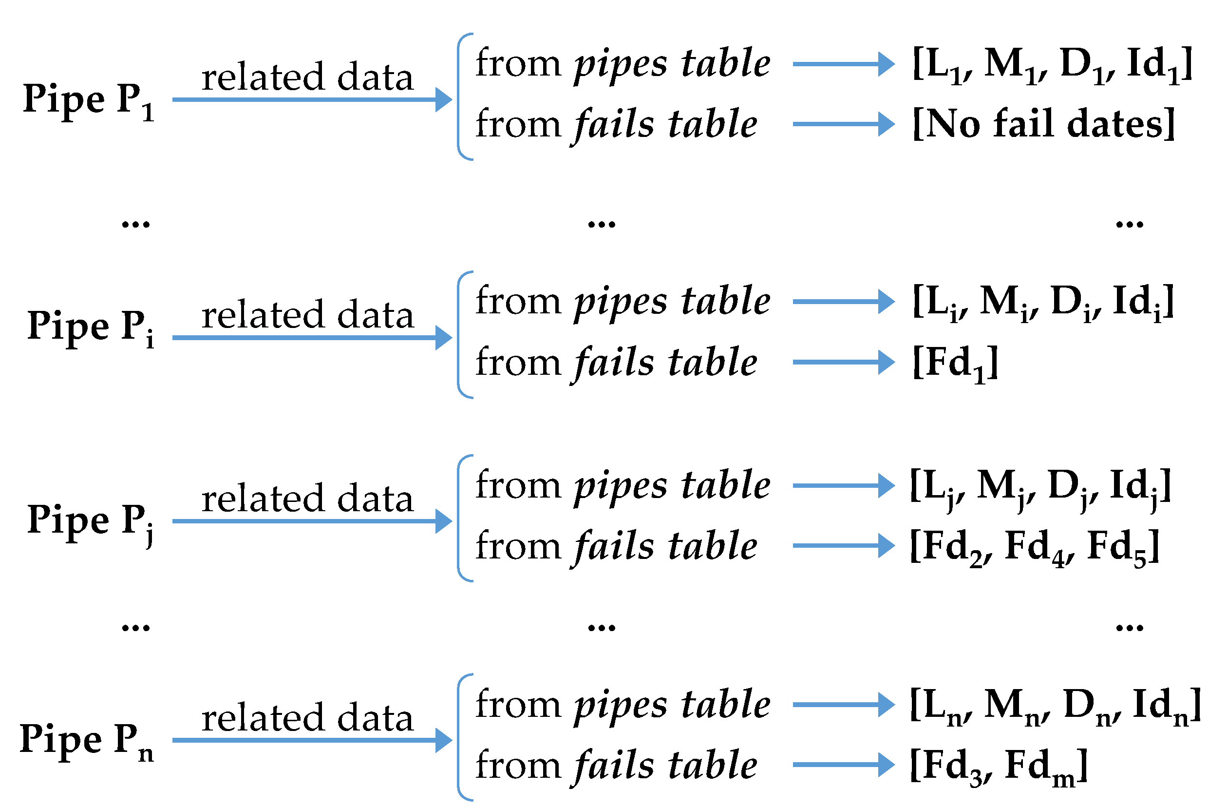
For the case of the four pipes taken as examples, Figure 3 shows the pipe data (distribution and origin) and Figure 4 shows the way the failure information is considered in the model.

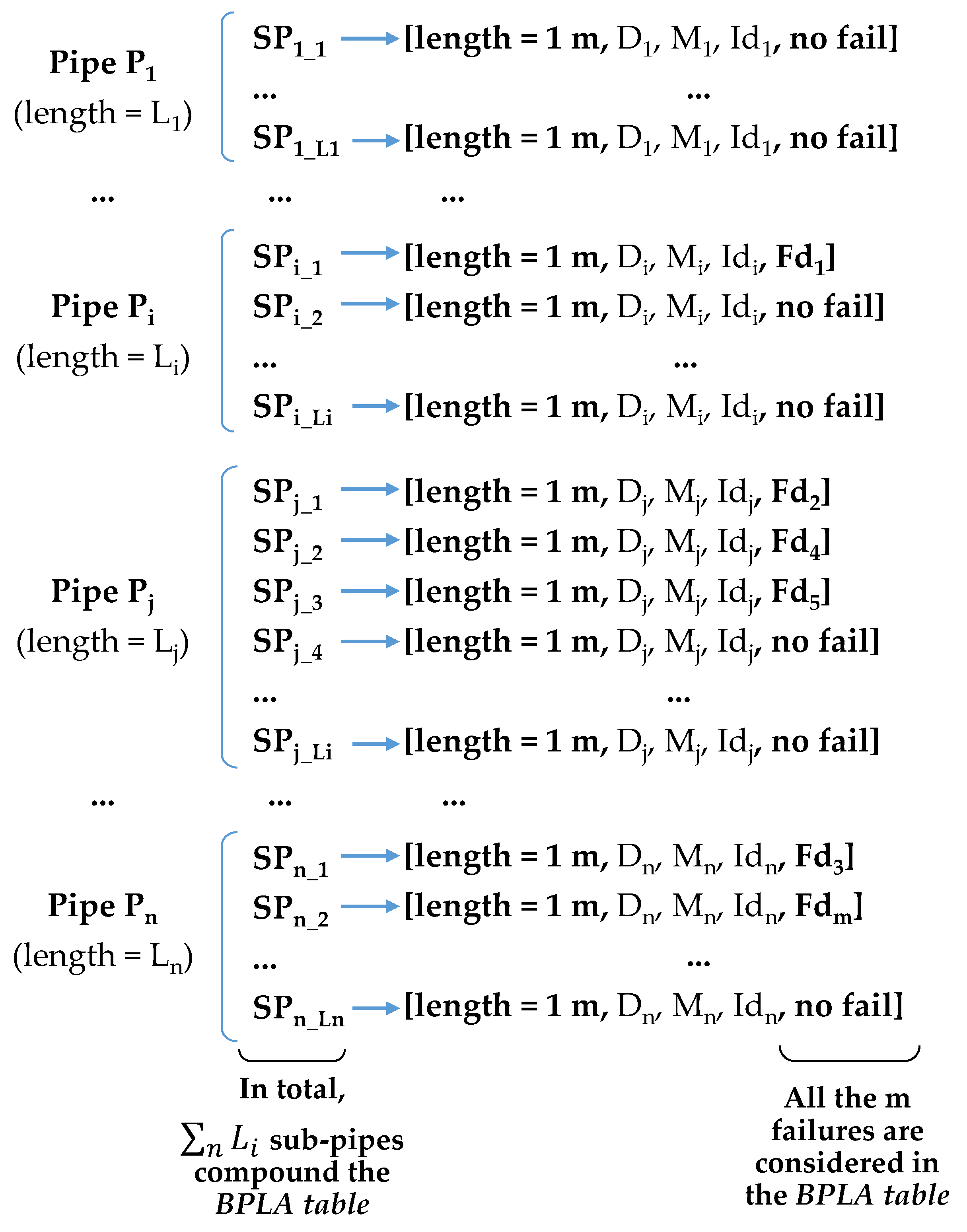
Regardless the total length of each one, pipe ${\mathrm{P}}_1$ had no failures during the time window, pipe ${\mathrm{P}}_{\mathrm{i}}$ had only 1 failure, and pipes ${\mathrm{P}}_{\mathrm{j}}$ and ${\mathrm{P}}_{\mathrm{n}}$ had 3 and 2 failures, respectively. For the BPLA model, each pipe, of length L, is divided into L sub-pipes of 1 meter-length, and each one of the failures recorded in the original pipe is assigned to one of the resulting sub-pipes. This way, all the failures are considered in the model, all the lengths of each original pipe are properly kept in the model, and each sup-pipe can be considered as a non-repairable element. One part of each pipe (the sub-pipes with assigned failures) is contributing to the failure function, but not the rest of it.

Figure 5 shows the generation of sub-pipes and the way pipe properties are transferred to them. The number of failures are distributed to the same number of sub-pipes, the rest remaining with no fails assigned. The outcome of this process is the BPLA table (

Table 3. Structure of the BPLA table.

Sub-Pipe	Length	Diam.	Mat.	Fail Date	Instal. Date	LtF	TtF
SP1_1	1	D1	M1	-	Id1	Ed − Id1	Ed − Sd
...	1	D1	M1	-	Id1	Ed − Id1	Ed − Sd
SP1_L1	1	D1	M1	-	Id1	Ed − Id1	Ed − Sd
...	...	...	...	...	...	...	...
SPi_1	1	Di	Mi	Fd1	Idi	Fd1 − Idi	Fd1 − Sd
SPi_2	1	Di	Mi	-	Idi	Ed − Idi	Ed − Sd
...	1	Di	Mi	-	Idi	Ed − Idi	Ed − Sd
SPi_Li	1	Di	Mi	-	Idi	Ed − Idi	Ed − Sd
SPj_1	1	Dj	Mj	Fd2	Idj	Fd2 − Idj	Fd2 − Sd
SPj_2	1	Dj	Mj	Fd4	Idj	Fd4 − Idj	Fd4 − Sd
SPj_3	1	Dj	Mj	Fd5	Idj	Fd5 − Idj	Fd5 − Sd
SPj_4	1	Dj	Mj	-	Idj	Ed − Idj	Ed − Sd
...	1	Dj	Mj	-	Idj	Ed − Idj	Ed − Sd
SPj_Lj	1	Dj	Mj	-	Idj	Ed − Idj	Ed − Sd
...	...	...	...	...	...	...	...
SPn_1	1	Dn	Mn	Fd3	Idn	Fd3 − Idn	Fd3 − Sd
SPn_2	1	Dn	Mn	Fd6	Idn	Fd6 − Idn	Fd6 − Sd
SPn_3	1	Dn	Mn	-	Idn	Ed − Idn	Ed − Sd
...	1	Dn	Mn	-	Idn	Ed − Idn	Ed − Sd
SPn_Ln	1	Dn	Mn	-	Idn	Ed − Idn	Ed − Sd

). Each row in this table corresponds to each sub-pipe, so that it is compounded by as many rows as the network length in meters—for this purpose, the actual length of each pipe should be rounded to the nearest whole number. As all the dates are transferred, the last two columns of the BPLA table can be calculated:

• $\mathrm{LtF}$ (life till failure) is the time elapsed between the installation date (Id) and the fail date (Fd) in case the sub-pipe has one failure assigned, or between the installation date (Id) and the end date (Ed) of the availability window in case the sub-pipe has not a failure assigned. Later analysis of $\mathrm{LtF}$ will provide the estimation for the average service life of the pipe group.
• $\mathrm{TtF}$ (time till failure) is the time elapsed between the start date (Sd) of the availability window and the fail date (Fd) in case the sub-pipe has one failure assigned, or between the start date (Sd) and the end date (Ed) of the availability window in case the sub-pipe has not a failure assigned. Analysis of $\mathrm{TtF}$ will provide the location on the bath curve and the hazard rate for future failures forecasting.

Finally, Figure 4 also shows the pre-BPLA approach [37], which could be understood as a simplified version of the BPLA. Pre-BPLA only takes into account the first failure occurred in each pipe, and discard the rest. In fact, this procedure is a straight application of the techniques of maintenance engineering to network pipes. It is simpler and faster than the BPLA, and therefore, more feasible for novel utilities. At the same time, the simplifications assumed biased the results in a greater extent. Results provided by the pre-PBLA model will secondarily be obtained and shown in the case study. However, because of the limited data it works with, the pre-BPLA should be kept apart in favor of the BPLA.

Statistical analysis: The BPLA table now contains all the relevant information for all the sub-pipes, of each pipe group, ready for the statistical analysis. Following a univariate parametric model, such analysis consists in finding the distribution that best fits the failure information contained in the BPLA table. The Weibull distribution is the first recommended candidate because of its characteristics and flexibility, and the one considered in this paper, though there are other possible options. Several techniques may be employed to perform the fitting—maximum likelihood estimation method, method of moment, least-squares regression method, graphical methods, etc. [38,39]. The outcome of the adjustment are the two specific parameters of the Weibull distribution—shape ($\mathsf{\beta }$) and scale ($\mathsf{\eta }$)—thus assuming that the location parameter ($\mathsf{\gamma }$) has no influence in this type of analysis. In consequence, $\mathrm{t}$ being the failure time for each sub-pipe, Equations (1) to (4) [40] show the failure behavior in each pipe group:

$$f\left(t\right)=\frac{\beta }{\eta }{\left(\frac{t}{\eta }\right)}^{\beta -1}{e}^{-{\left(\frac{t}{\eta }\right)}^{\beta }}$$

(1)

$$F\left(t\right)=1-e^{-{\left(\frac{t}{\eta }\right)}^{\beta }}$$

(2)

$$S\left(t\right)=e^{-{\left(\frac{t}{\eta }\right)}^{\beta }}$$

(3)

$$\lambda \left(t\right)=\frac{\beta }{\eta }{\left(\frac{t}{\eta }\right)}^{\beta -1}$$

(4)

Equation (1) is the failure probability (probability density function), Equation (2) is the failure function (cumulative distribution function), Equation (3) is the survival function (complementary cumulative distribution function) and Equation (4) is the failure rate (hazard function).

Each failure time should be accounted since the pipe installation moment (LtF) or since the time window onset (TtF). Then, as advanced above, the statistical analysis will be performed independently on each of them. In consequence, the results finally obtained will be two sets of Equations (1) to (4), one per each time variable considered.

Once each analysis is completed, and before coming to any first conclusion, the goodness of fit must be checked. There are several techniques available—chi-squared, Kolmogorov–Smirnov, etc. [38,39,40,41]. In case they do not validate the Weibull fitting, other distributions could be tested; for example, normal, log-normal, or gamma.

Interpretation of results: Two Weibull parameters are obtained after each fitting: shape and scale for LtF (denoted as ${\mathsf{\beta }}_{\mathrm{LtF}}$ and ${\mathsf{\eta }}_{\mathrm{LtF}}$) and, also, shape and scale for TtF (denoted as ${\mathsf{\beta }}_{\mathrm{TtF}}$ and ${\mathsf{\eta }}_{\mathrm{TtF}}$). Their meanings are quite direct because of the characteristics of the Weibull distribution itself.

The scale factor, $\mathsf{\eta }$, is generally called characteristic life. It is not the mean life of the distribution, but the life that is reached by the 63.2% of the units. Therefore, for the LtF distribution, the ${\mathsf{\eta }}_{\mathrm{LtF}}$ provides a quick assessment of the age at which each meter of pipe will likely have its first failure.

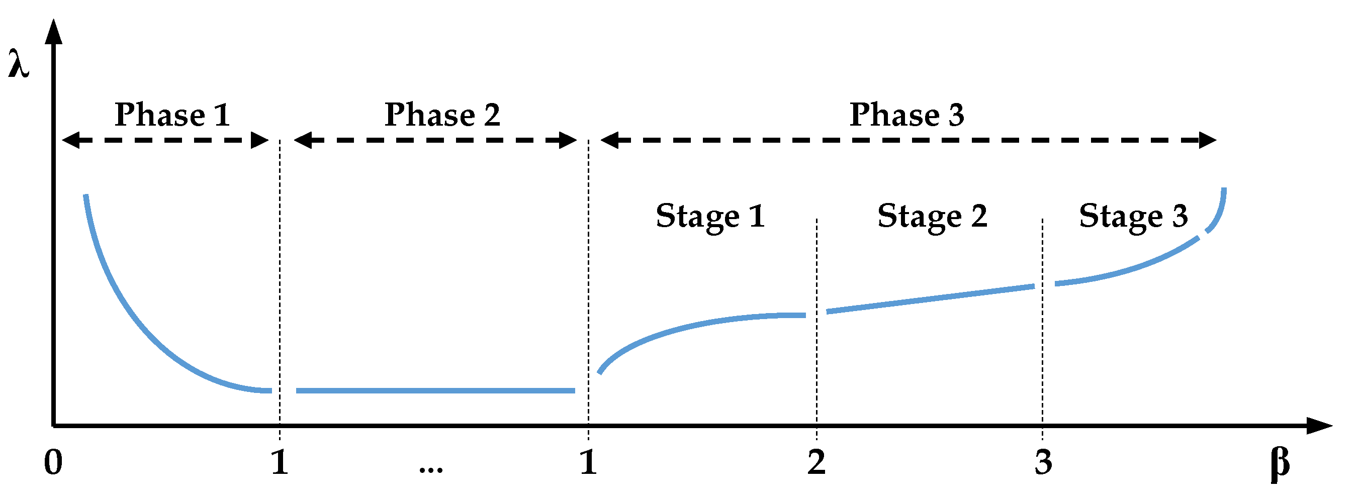
In maintenance engineering, the shape factor, $\mathsf{\beta }$, is closely related to the failure rate, $\mathsf{\lambda }$, (Figure 6) and, in consequence, to the bath curve [32]. Taking advantage of the variable TtF, for which all the sub-pipes have been analyzed from the same time onset, the shape parameter ${\mathsf{\beta }}_{\mathrm{TtF}}$ and the failure rate ${\mathsf{\lambda }}_{\mathrm{TtF}}$ (Equation (4)) are now known. According to Figure 6, the value of the ${\mathsf{\beta }}_{\mathrm{TtF}}$ will show the location of the pipe group onto the bath curve. This way, the kind of failures that are currently occurring on the pipe group can be categorized as early, useful or wearout life, and utility managers may set future planning according to this. Secondly, based on the value of ${\mathsf{\lambda }}_{\mathrm{TtF}}$, a prediction of the number of future expected failures can be made for the pipe group. It is assumed that this calculation should be limited to the short-term. It will be valid as long as the location on the bath curve does not change from one stage to the next one. In case it happens, that would be unveiled by a new value of ${\mathsf{\beta }}_{\mathrm{TtF}}$, that, in turn, should be the one considered for a new calculation.

2.2. Quick Summary of the WPHM

The WPHM is a well-known semi-parametric model (Figure 1) that is taken as a reference in this work for comparison purposes. Only some main features are summarized below. Full information on the WPHM is available in the literature [3,10,15,16,17,18,19].

One main different is that the WPHM does not require the network pipes to be categorized in homogeneous groups. Instead, all the pipes may be kept in the same table because the particular features of each one are taken by the model as explicative covariates; after the calculation, its influence will be assessed through particular coefficients.

The second difference is the, more complex, way the failure data is organized, combined with the pipe data and, processed. As shown in Figure 7, the WPHM focuses on the so-called interarrival time ($\mathsf{\tau }$). This is, for each failure in each pipe, the time elapsed since the immediately preceding failure occurred. For the case of the first recorded failure, it is the time since the onset of the time window. After the last recorded failure, one additional interarrival time is considered—the time between the last failure and the end of the time window. This last interarrival time is treated as censored (it ends at the end of the time window, not at a new failure) while the others are treated as uncensored (they end at the next failure) [32]. If all the failures in all the pipes are processed in this way, the final table obtained, here called WPHM table, will have the structure shown in

Table 4. Structure of the Weibull proportional hazard model (WPHM) table.

$\mathsf{\tau }$	Fail Date	Pipe	Fail Order in Pipe	Interarr. Time	AL	Length	Diam.	Mat.
$\tau$1	-	P1	-	Ed − Sd	Sd − Id1	L1	D1	M1
...	...	...	...	...	...	...	...	...
$\tau$i	Fd1	Pi	Pi_O1	Fd1 − Sd	Sd − Idi	Li	Di	Mi
$\tau$i + 1	-	Pi	-	Ed − Fd1	Fd1 − Idi	Li	Di	Mi
$\tau$i + 2	Fd2	Pj	Pj_O1	Fd2 − Sd	Sd − Idj	Lj	Dj	Mj
$\tau$i + 3	Fd4	Pj	Pj_O2	Fd4 − Fd2	Fd2 − Idj	Lj	Dj	Mj
$\tau$i + 4	Fd5	Pj	Pj_O3	Fd5 − Fd4	Fd4 − Idj	Lj	Dj	Mj
$\tau$i + 5	-	Pj	-	Ed − Fd5	Fd5 − Idj	Lj	Dj	Mj
...	...	...	...	...	...	...	...	...
$\tau$m + n − 2	Fd3	Pn	Pn_O1	Fd3 − Sd	Sd − Idn	Ln	Dn	Mn
$\tau$m + n − 1	Fdm	Pn	Pn_O2	Fdm − Fd3	Fd3 − Idn	Ln	Dn	Mn
$\tau$m + n	-	Pn	-	Ed − Fdm	Fdm − Idn	Ln	Dn	Mn

(consistent with Table 1 and Table 2). Each row contains the information of each interarrival time and, additionally, the additional information (covariates) of the pipe in which that failure occurred.

The population formed by all the interarrival times, organized in the vector $\mathrm{T}\left({\mathsf{\tau }}_1,{\mathsf{\tau }}_2,\dots ,{\mathsf{\tau }}_{\mathrm{m}+\mathrm{n}}\right)$, may be described by a Weibull distribution and that vector may be related to the vector of the covariates $\mathrm{X}\left({\mathrm{x}}_1,{\mathrm{x}}_2,\dots ,{\mathrm{x}}_{\mathrm{q}}\right)$ as shown by Equation (5) [15]:

$$\ln T=\beta \times X+\sigma \times W$$

(5)

where $\mathsf{\beta }$ is the vector that contains the covariates coefficients, $\mathrm{W}$ is the vector of the random errors and $\mathsf{\sigma }$ is a regression parameter.

Each coefficient ${\mathsf{\beta }}_0,{\mathsf{\beta }}_1,{\mathsf{\beta }}_2,\dots ,{\mathsf{\beta }}_{\mathrm{q}}$, shows the influence of each covariate, ${\mathrm{x}}_1,{\mathrm{x}}_2,\dots ,{\mathrm{x}}_{\mathrm{q}}$, on the failure occurrences $\mathrm{T}$. Yet, the more relevant parameters are ${\mathsf{\beta }}_0$ and $\mathsf{\sigma }$, which are called respectively intercept and scale. This notation is purposely kept the same as the one usually found in the literature [15,16], and therefore, it should be remarked that while both coefficients are not the same as those already defined for the BPLA, they are closely related to them. The reason for this is that the Weibull distribution lays on the core of both methodologies. In particular the relation between the coefficients employed by both models is [42]:

$$Intercept={\beta }_0=\ln \left({\eta }_{TtF}\right)$$

(6)

$$Scale=\sigma =\frac{1}{{\beta }_{TtF}}$$

(7)

The number of the future expected failures can also be predicted through the WPHM. However, it entails a more complex calculation. It is performed through Equation (8) [15] and a Monte Carlo simulation process. In summary, for each pipe, random values (up to 1000) of $\mathrm{S}$ (survival) are produced and the corresponding interarrival time, $\mathsf{\tau }$, for each value is obtained. With each iteration, the $\mathsf{\beta }$ coefficients influence each new $\mathsf{\tau }$. Eventually, the end of the simulation period is reached and the calculations are performed again for the following pipe of the network.

$$\tau ={\left(\ln \left(\frac{1}{S}\right)e^{\left(\frac{\beta ·X}{\sigma }\right)}\right)}^{\sigma }$$

(8)

Finally, the results obtained for each pipe are added up to get the final single figure—the total failures. Equation (9) shows the total failures during the first year of the simulation for each pipe group, $\mathrm{m}\left({\mathrm{T}}_0,{\mathrm{T}}_1\right)$, where ${\mathrm{T}}_0$ is the current year, ${\mathrm{T}}_1$ is that first year,$\mathrm{p}$ is the order number of each pipe within the group, ${\mathrm{m}}_{\mathrm{p}}$ is the number of failures of pipe $\mathrm{p}$ and ${\mathrm{n}}_{\mathrm{p}}$is the total number of pipes in the group. By extending the simulation time one more year and detracting the failures occurred up to the year before, the increment of total failures for each successive year can be easily obtained through Equations (9) and (10) [16].

$$m\left(T_0, T_1\right)={\displaystyle \sum }_{p=1}^{n_p}{m}_p\left(T_0, T_1\right)$$

(9)

$$m\left(T_{i-1}, T_i\right)={\displaystyle \sum }_{p=1}^{n_p}{m}_p\left(T_0, T_i\right)-{\displaystyle \sum }_{p=1}^{n_p}{m}_p\left(T_0, T_{i-1}\right)$$

(10)

3. Case Study and Results

3.1. Basic Description of the System

The BPLA model has been implemented in a real network located in the eastern part of Spain. It is about 1000 km long and supplies water to more than 500,000 people. The authors have been collaborating with this particular utility for more than twenty years in different areas such as hydraulic modeling, metering and losses management, demand characterization, etc. Although failure records have been recorded during several decades, the organization of these data was not oriented to be used in these type of modelling. Only recently the information collection has been focused towards the here depicted methodology. Therefore, only two years (2017 and 2018) are reliably available at the moment, which, on the other hand, is representative of a number of other small- and medium-sized utilities the authors also collaborate with, both in Spain and abroad. Despite the restriction in data, the results obtained below are consistent and already provide valuable information for the planning that managers daily face. As the information from new years is added and that from old years is refined, these results will be better, but not more numerous, at least without limiting new developments currently under way.

Table 5. Distribution of network pipe materials.

Materials	Network Length (%)	Avg. Age (Years)
Asbestos cement (AC)	30.2	41.4
Ductile iron (DI)	26.0	45.4
Cast iron (CI)	17.4	62.8
Polyethylene (PE)	25.5	42.7
Other (steel, PVC, concrete…)	0.9	55.7

shows the main pipe materials installed in the network as well as the length percentage for each one and its average age.

Table 6. Distribution of network pipe diameters per groups.

Diameter Groups		Network Length (%)
ID Gr.	Diameter (mm)
1	<63	6.0
2	63–140	47.6
3	140–200	23.3
4	200–280	13.5
5	280–400	4.5
6	>400	5.1

shows the groups in which the network diameters have been classified as well as the length percentage for each group.

The original fails table for all four main materials (“Other” are already excluded here) has 745 records for both years. Fails distribution can be better understood if all the fails are classified, per year, among the four main groups of materials and all six groups of diameters (

Table 7. Pipe failure information.

Year	Material Gr.				Diameter Gr.
	AC	DI	CI	PE	1	2	3	4	5	6
2017	70	27	57	192	61	227	33	25	0	0
2018	46	52	61	240	131	219	38	9	2	0
Total	116	79	118	432	193	446	71	34	2	0

).

3.2. Application and Results of BPLA

The BPLA works on pipe groups of homogeneous characteristics. In this case, such groups (

Table 8. Pipe groups selected for the first analysis.

Pipe Group	Mat. Gr./Diam. Gr.	Total Pipes	Total Length (km)	Recorded Failures
				Pipes with Failures	Total Failures
1	AC/2	6149	165.7	62	75
2	DI/2	8278	121.4	56	58
3	CI/2	5242	120.1	70	87
4	PE/2	5382	138.1	166	232

) have been defined according to three criteria:

-

Homogeneity within each pipe group will be based on the combination of same material and same diameter. The age is only being taken into account in case the results are not statistically acceptable.

-

All four main materials must be represented in the pipe groups.

-

For each material, the diameter group chosen will be the one with the highest number of recorded failures.

Once the pipe groups have been defined, the particular pipes tables Table 1 and fails tables (Table 2) for each one must be prepared. Then, the pipes contained in the pipes table are split in 1 m-length sup-pipes, and the failures are distributed among them as explained above. The result is the so-called PBLA table (Table 3) for each group. It should be noticed that the BPLA table is compounded by as many rows as the total length of the pipes in each group (Table 8) in meters, yet only a few of them, in comparison, have been assigned one failure.

In this case, the analysis has been performed through the software R [42]. The Weibull parameters obtained for each group are shown in

Table 9. Weibull parameters after the first analysis.

Pipe Group	LtF Analysis		TtF Analysis
	${\mathsf{\beta }}_{\mathbf{L}\mathbf{t}\mathbf{F}}$	${\mathsf{\eta }}_{\mathbf{L}\mathbf{t}\mathbf{F}}$	${\mathsf{\beta }}_{\mathbf{T}\mathbf{t}\mathbf{F}}$	${\mathsf{\eta }}_{\mathbf{T}\mathbf{t}\mathbf{F}}$
1	8.03	114.2	0.98	8700
2	9.96	108.8	1.33	635
3	4.76	197.6	1.27	1123
4	7.08	115.0	1.18	436

. Before going further, the goodness of the fitting was checked by the Kolmogorov–Smirnov (K-S) test [38,39,40,41]. As the results of the test show (

Table 10. Goodness of fitting test results (K-S) after the first analysis.

Pipe Group	LtF Analysis			TtF Analysis
	${\mathbf{D}}_{\mathbf{M}\mathbf{a}\mathbf{x}}$	${\mathbf{D}}_{\mathbf{C}\mathbf{r}\mathbf{i}\mathbf{t}}$	$\left({\mathbf{D}}_{\mathbf{M}\mathbf{a}\mathbf{x}}<{\mathbf{D}}_{\mathbf{C}\mathbf{r}\mathbf{i}\mathbf{t}}\right)?$	${\mathbf{D}}_{\mathbf{M}\mathbf{a}\mathbf{x}}$	${\mathbf{D}}_{\mathbf{C}\mathbf{r}\mathbf{i}\mathbf{t}}$	$\left({\mathbf{D}}_{\mathbf{M}\mathbf{a}\mathbf{x}}<{\mathbf{D}}_{\mathbf{C}\mathbf{r}\mathbf{i}\mathbf{t}}\right)?$
1	0.0092	0.0034	No	0.0001	0.0034	Yes
2	0.0002	0.0038	Yes	0.0001	0.0039	Yes
3	0.0554	0.0043	No	0.0003	0.0043	Yes
4	0.0005	0.0036	Yes	0.0001	0.0036	Yes

), the fitting for variable LtF in groups 1 and 3 was not acceptable.

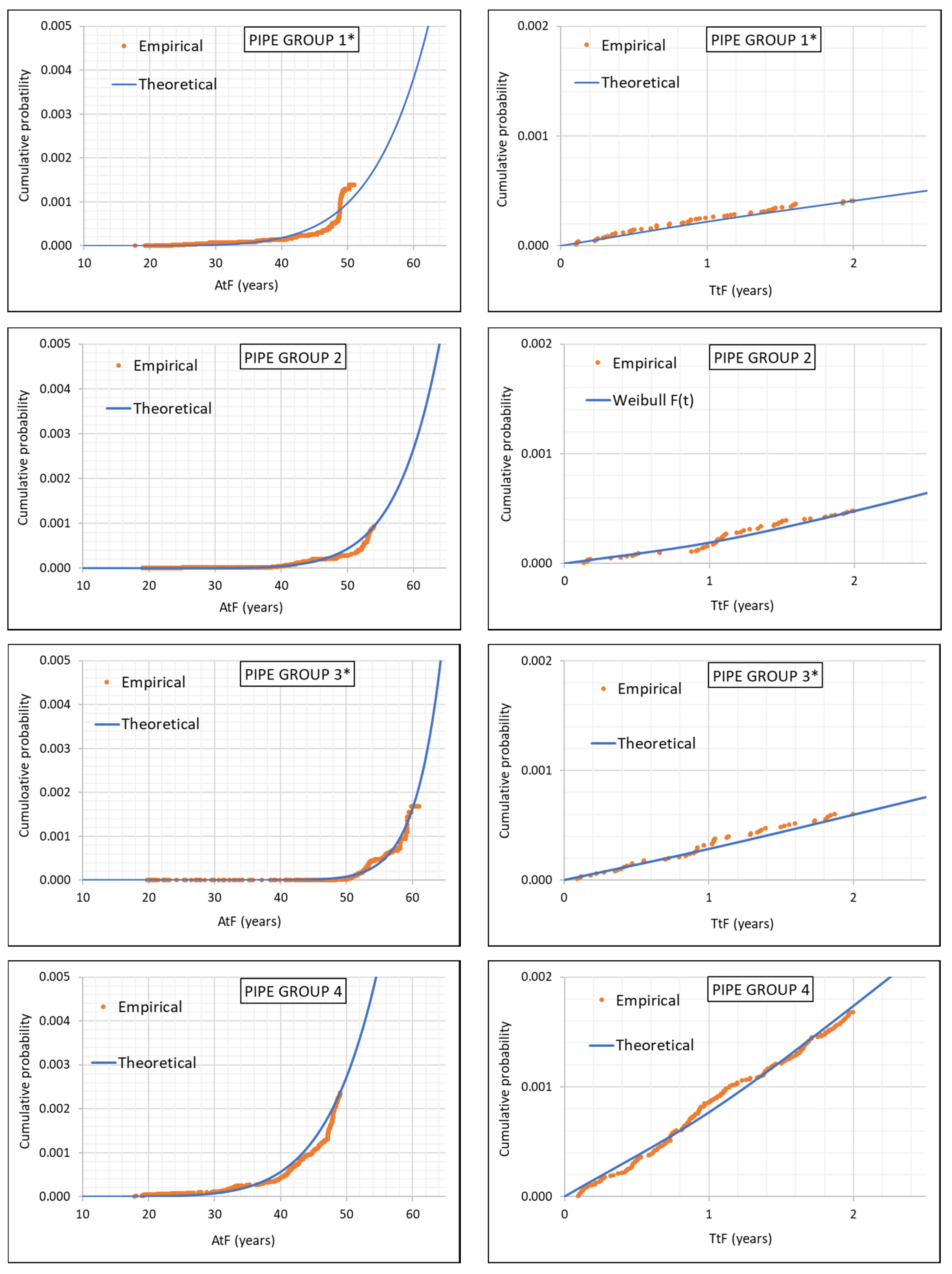
Solution came by modifying pipe groups 1 and 3, and adding one more criterion based on the age of pipes—only pipes younger than 50 years will be included in group 1, and pipes younger than 60 years will be included in group 3. Hereon, the two modified groups are denoted as 1* and 3*.

Table 11. Pipe groups selected for the second analysis (changes in 1 and 3).

Pipe Group	Mat. Gr./Diam. Gr./Age Gr.	Total Pipes	Total Length (km)	Recorded Failures
				Pipes with Failures	Total Failures
1*	AC/2/<50	156,397	156.4	52	64
2	DI/2/all	121,443	121.4	56	58
3*	CI/2/<60	84,694	84.7	36	51
4	PE/2/all	138,141	138.1	166	232

shows the data for the new pipe groups. Results of the Weibull parameters and goodness of fitting after the second analysis are shown in

Table 12. Weibull parameters after the second analysis.

Pipe Group	LtF Analysis		TtF Analysis
	${\mathsf{\beta }}_{\mathbf{L}\mathbf{t}\mathbf{F}}$	${\mathsf{\eta }}_{\mathbf{L}\mathbf{t}\mathbf{F}}$	${\mathsf{\beta }}_{\mathbf{T}\mathbf{t}\mathbf{F}}$	${\mathsf{\eta }}_{\mathbf{T}\mathbf{t}\mathbf{F}}$
1*	7.48	126.3	0.90	11,600
2	9.96	108.8	1.33	635
3*	16.36	88.9	1.07	2,070
4	7.08	115.0	1.18	436

and

Table 13. Goodness of fitting test results (K-S) after the second analysis.

Pipe Group	LtF Analysis			TtF Analysis
	${\mathbf{D}}_{\mathbf{M}\mathbf{a}\mathbf{x}}$	${\mathbf{D}}_{\mathbf{C}\mathbf{r}\mathbf{i}\mathbf{t}}$	$\left({\mathbf{D}}_{\mathbf{M}\mathbf{a}\mathbf{x}}-{\mathbf{D}}_{\mathbf{C}\mathbf{r}\mathbf{i}\mathbf{t}}\right)?$	${\mathbf{D}}_{\mathbf{M}\mathbf{a}\mathbf{x}}$	${\mathbf{D}}_{\mathbf{C}\mathbf{r}\mathbf{i}\mathbf{t}}$	$\left({\mathbf{D}}_{\mathbf{M}\mathbf{a}\mathbf{x}}-{\mathbf{D}}_{\mathbf{C}\mathbf{r}\mathbf{i}\mathbf{t}}\right)?$
1*	0.0004	0.0034	Yes	5 × 10−5	0.0034	Yes
2	0.0002	0.0038	Yes	0.0001	0.0039	Yes
3*	0.0005	0.0046	Yes	0.0001	0.0046	Yes
4	0.0005	0.0036	Yes	0.0001	0.0036	Yes

, respectively. Finally, the K-S test yields positive results and the new Weibull distributions can be reliably considered as good descriptions of the failures time-evolution for all four groups. Figure 8 shows the comparison between the empirical and theoretical cumulative distribution functions [43].

Once the Weibull parameters have been obtained, the three sought results for each pipe group can be derived from them. The characteristic life and the position on the bath curve come directly from ${\mathsf{\eta }}_{\mathrm{LtF}}$ and ${\mathsf{\beta }}_{\mathrm{TtF}}$, respectively. In particular, depending on the position spotted by ${\mathsf{\beta }}_{\mathrm{TtF}}$, a general recommendation could be set for the network managers in relation to the kind of actions to be planned in the near future (

Table 14. BPLA results.

Pipe Group	Characteristic Life (Years)	${\mathbf{\beta }}_{\mathit{T}\mathit{t}\mathit{F}}$	Location on the Bath Curve		Recommened Action
			Stage	Phase
1*	126.3	0.90	1	-	Corrective
2	108.8	1.33	3	1	Preventive
3*	88.9	1.07	3	1	Preventive
4	115.0	1.18	3	1	Preventive

).

A comment should be made on group 1*, which shows a much younger appearance than could be expected for the pipes that form it. The reason relies on the added condition on age (< 50 years), and on the short network information available (only 2 years)—in fact, pipe group 1* is a sub-group artificially younger than the original group 1. In any case, it must be reminded that the main aim is to compare the new simple method (BPLA) with a complex one (WPHM) by showing that, for the same data, the results provided by the first one are equivalent to those provided by the second one.

Finally, based on ${\mathsf{\beta }}_{\mathrm{TtF}}$, the hazard rate, ${\mathsf{\lambda }}_{\mathrm{TtF}}$, for each year and pipe group is obtained and, according to it, the expected number of future failures can be calculated (

Table 15. BPLA failure forecast for the upcoming years.

Pipe. Group	Year 1		Year 2		Year 3		Year 4		Year 5
	${\mathsf{\lambda }}_{\mathbf{T}\mathbf{t}\mathbf{F}}$	#Fails	${\mathsf{\lambda }}_{\mathbf{T}\mathbf{t}\mathbf{F}}$	Fails	${\mathsf{\lambda }}_{\mathbf{T}\mathbf{t}\mathbf{F}}$	Fails	${\mathsf{\lambda }}_{\mathbf{T}\mathbf{t}\mathbf{F}}$	Fails	${\mathsf{\lambda }}_{\mathbf{T}\mathbf{t}\mathbf{F}}$	Fails
1*	2.0 × 10−4	31	1.8 × 10−4	29	1.8 × 10−4	28	1.7 × 10−4	27	1.7 × 10−4	26
2	2.5 × 10−4	30	3.1 × 10−4	38	3.6 × 10−4	43	3.8 × 10−4	48	4.2 × 10−4	51
3*	3.0 × 10−4	26	3.2 × 10−4	27	3.3 × 10−4	28	3.3 × 10−4	28	3.4 × 10−4	29
4	9.1 × 10−4	125	1.0 × 10−3	142	1.1 × 10−3	153	1.2 × 10−3	161	1.2 × 10−3	167

).

3.3. Application and results of WPHM

As explained above, when applying the WPHM, the pipes table and the fails table should be combined in a specific way, so that each interarrival time is contained in each row of the final WPHM table. Four basic strata for four main materials has been kept here, and therefore, all four pipe groups have been kept independent for comparison purposes.

According to the pipe information available, the explanatory covariates considered are the following:

-

Logarithm of pipe length (Ln.length): Following Martins [34], the logarithm of the length has been considered (instead of the length itself as Alvisi and Franchini do [16,37]) assuming that the hazard rate should be proportional to the length of the pipe—which is a suitable assumption for the particular network under study.

-

Diameter (Diam.): In all four pipe groups, pipes belong to the diameter group 2 (Table 6).

-

Total number of failures (Fails): This covariate is constant for each pipe, and, therefore, for all the interarrival times derived from it. As explained by Martins [34], this is a much practical way of keeping it in the analysis, as opposed to other options, such as neglecting it [16] or taking it as a dynamic covariate [15], which could cause convergence problems in the subsequent Monte Carlo simulations.

-

Age left (AL): As shown in Figure 7, this is a dynamic covariate that takes a different value for each interarrival time on the same pipe.

Once the WPHM table is ready for each pipe group, the statistical analysis was performed through the R software [42]. The results obtained are shown in

Table 16. WPHM Results.

Coefficient	Pipe Group 1*		Pipe Group 2		Pipe Group 3*		Pipe Group 4
	$\mathsf{\beta }$	${\mathbf{e}}^{\mathsf{\beta }}$	$\mathsf{\beta }$	${\mathbf{e}}^{\mathsf{\beta }}$	$\mathsf{\beta }$	${\mathbf{e}}^{\mathsf{\beta }}$	$\mathsf{\beta }$	${\mathbf{e}}^{\mathsf{\beta }}$
Intercept (${\mathsf{\beta }}_0$)	5.38	-	8.15	-	20.07	-	3.81	-
Scale ($\mathsf{\sigma }$)	1.18	-	0.58	-	1.30	-	0.88	-
Ln.length $({\mathsf{\beta }}_1)$	−0.206	0.813	−0.287	0.750	−0.174	0.839	−0.236	0.789
Diam (${\mathsf{\beta }}_2$)	0.006	1.006	−0.022	0.977	−0.065	0.937	0.016	1.016
Fails (${\mathsf{\beta }}_3$)	−3.319	0.036	−2.353	0.095	−2.497	0.082	−0.728	0.482
AL (${\mathsf{\beta }}_4$)	0.041	1.042	−0.025	0.974	−0.109	0.896	−0.024	0.975

.

The main result for the purpose of this work is the scale ($\mathsf{\sigma }$) parameter, since it is closely related to the results provided by the BPLA method, particularly to the ${\mathsf{\beta }}_{\mathrm{TtF}}$ paremeter.

Table 17. WPHM scale parameters converted to the BPLA approach

Pipe Group	Scale	${\mathsf{\beta }}_{\mathbf{T}\mathbf{t}\mathbf{F}}^{\mathbf{e}\mathbf{q}\mathbf{u}\mathbf{i}\mathbf{v}}$
1*	1.18	0.847
2	0.58	1.724
3*	1.30	0.769
4	0.88	1.136

shows the value of that parameter for each pipe group once they have been converted to its equivalent under the BPLA approach (Equation (7)).

The rest of parameters in Table 16 show the importance and influence of the covariates on the interarrival times distribution. The negative values for Ln.length and Fails, in all four groups, are quite consistent—they mean an inverse relation between an increment in the covariate and an increment in the time between failures. In other words, the longer the pipe or the greater the number of failures it had, the shorter the time between failures will become. The exponential of the coefficient confirms a much greater influence of #Fails, compared to Ln.length, since the value for the second one is closer to 1 (marginal contribution [34]). Coefficients of Diam. seem to be less consistent—two of them positive and two negative—but considering that all pipe groups are restricted to a (relatively) narrow diameters range (group 2), that apparent fine accuracy within the group is not much relevant. The case of AL is more important. Whereas its coefficient turns out to be quite consistent for pipe groups 2, 3* and 4. In summary, the older the pipe, the shorter the fail time; this does not seem the case for group 1*. That positive sign would indicate that the failures of pipe group 1* would be those of young pipes (early kind). Obviously, the original pipe group 1 was not made up by young pipes, but it had to be modified to group 1* by removing the oldest pipes (>50 years) for statistical fitting purposes, and that has shown an effect on the AL coefficient. This conclusion is very much related to the results obtained by the BPLA model and will deserve some further explanation in the next section.

From the statistical fitting just made, it is possible to undertake the next stage of the WPHM—the calculation of expected failures in the future years. As summarized in the previous section, (Equations (8) to (10)), the procedure is based on a Monte Carlo simulation on each single pipe [15]. By adding the results obtained for all the pipes in each group, final figures obtained are shown in

Table 18. WPHM Failure forecast for the upcoming years.

Pipe Group	Year 1	Year 2	Year 3	Year 4	Year 5
1*	35	30	29	28	26
2	18	34	44	52	59
3*	35	30	30	31	34
4	113	130	138	144	147

.

4. Discussion

The developments and case study presented can be discussed from two perspectives. The first one is the quality standard of the results obtained. That would back the utility of the BPLA model for the aim it has been devised. The second one is the effectiveness of the procedure in terms of resources and means required. That would make the BPLA model the intended convenient tool for the intended kind of target users.

4.1. Comparison of Results

The use of a new statistical model should be backed by two complementary analyses: sensitivity of results and validation of forecasts. However, such analyses could not be undertaken in a proper way in this case due to the scarce available data. As explained above, the BPLA is based on groups of pipes with homogeneous characteristics or, in real terms, as uniform as possible. At the same time, the least amount of recorded failures for each group must be 30. The full data available (two years) have been roughly enough to complete the pipes groups with the required number of failures (especially for first failures of group 3*, Table 11). Therefore, the balance between data homogeneity and data amount for each group has been considered as achieved, but no additional data is left available for the mentioned analysis.

As is often the case, the sensitivity analysis could be performed by making different pipe groups within each category (material and diameter range) and then by comparing the analysis performed on them. However, all the (failures) data available have been needed for the analysis done, and no more data is left to try different groupings. The only possibility would be to extend the range of diameters included in each group. However, that will decrease the homogeneity of the characteristics of the pipes within the group and it can be expected that the results will be, probably, worse and, certainly, less representative.

In the same way, the validation of forecasts should be done by using only the older data to perform the analysis and forecast, and then compare the first years forecasted with the more recent failure data. Again, all the failure data recorded for two years have been fully used to solve the model and to make the forecasts, so they could not reliably be contrasted until a few of years (two or three at least) have passed.

The problems found for proper sensitivity analysis and validation have driven to an alternative procedure. This is the reason why the WPHM has been considered. As a well known and extensively used model, the consistency between the results of the WPHM and the BPLA might imply a first-hand recognition for the reliability of the BPLA. Thus, there would not be such an essential need to wait several years before the amount of data available be increased.

The main comparison should focus on the numerical results obtained by both methodologies, and the first significant result is the characterization of the failure rate of each pipe group. In other words, its location on the bath curve (Figure 6).

Table 19. Summary and comparison of $\mathsf{\beta }$ parameters obtained by each model.

Pipe Group	$\mathsf{\beta }$ Obtained by Each Model			Relative Error (%) to WPHM
	WPHM	BPLA	Pre-BPLA	BPLA	Pre-BPLA
1*	0.85	0.90	0.87	6	2
2	1.72	1.33	1.33	23	23
3*	0.77	1.07	0.93	39	21
4	1.14	1.18	1.12	4	2

summarizes such results; those for WPHM have been extracted from Table 17, those for BPLA are extracted from Table 14, and the results for the pre-PBLA model can be found in Ramirez [37]. In addition, the relative errors for BPLA and pre-BPLA results with respect to WPHM results are also shown. In average, BPLA and WPHM differ in about 15%. This is can be considered as a positive conclusion, moreover, when considering that the location on the bath curve is set by ranges for $\beta$, and not by its exact value.

The second comparison focuses on the failure forecasting for the next five years. Though the main model proposed is the BPLA, the results obtained by WPHM are to be compared not only with BPLA, but also, again, with pre-BPLA. The reason for this is to notice the small discrepancies between the two, especially considering their essential differences, explained above.

Table 20. Failures forecasted for next five years by each model.

Pipe Gr.	WPHM					BPLA					pre-BPLA
	1	2	3	4	5	1	2	3	4	5	1	2	3	4	5
1*	35	30	29	28	26	31	29	28	27	26	25	23	21	21	20
2	18	34	44	52	59	30	38	43	48	51	31	38	44	48	52
3*	35	30	30	31	34	26	27	28	28	29	18	17	16	16	16
4	113	130	138	144	147	125	142	153	161	167	86	94	98	102	104

presents a summary of such results; those for WPHM have been extracted from Table 18, those for BPLA have been extracted from Table 15, and those for pre-BPLA can be found in Ramirez [37].

The relative errors of BPLA (and pre-BPLA), failure forecasts with respect to those of WPHM have been calculated (

Table 21. Relative errors (%) on failure forecasting for BPLA and pre-BPLA compared to WPHM.

Pipe Gr.	BPLA					pre-BPLA
	1	2	3	4	5	1	2	3	4	5
1*	11	3	3	4	0	32	24	29	26	23
2	67	12	2	8	14	43	11	0	8	14
3*	26	10	7	10	15	65	48	50	54	62
4	11	9	11	12	14	22	25	26	26	26

). The figures obtained remain at an acceptable level—in average, BPLA forecasts differ in about 12% from those of WPHM. In fact, an overview of the table highlights that year 1 is a particular case, especially for group 2. If that first year (even only group 2) was neglected, the error between both models would fall up to 8% or 9%. Being the failure forecasting a more sensitive calculation compared to that for the β parameter, the simplifications assumed for pre-BPLA become more visible, and the reliability gap between BPLA and pre-BPLA naturally increases. The average error of pre-BPLA compared to WPHM rises up to about 30%.

4.2. Comparison of Procedures

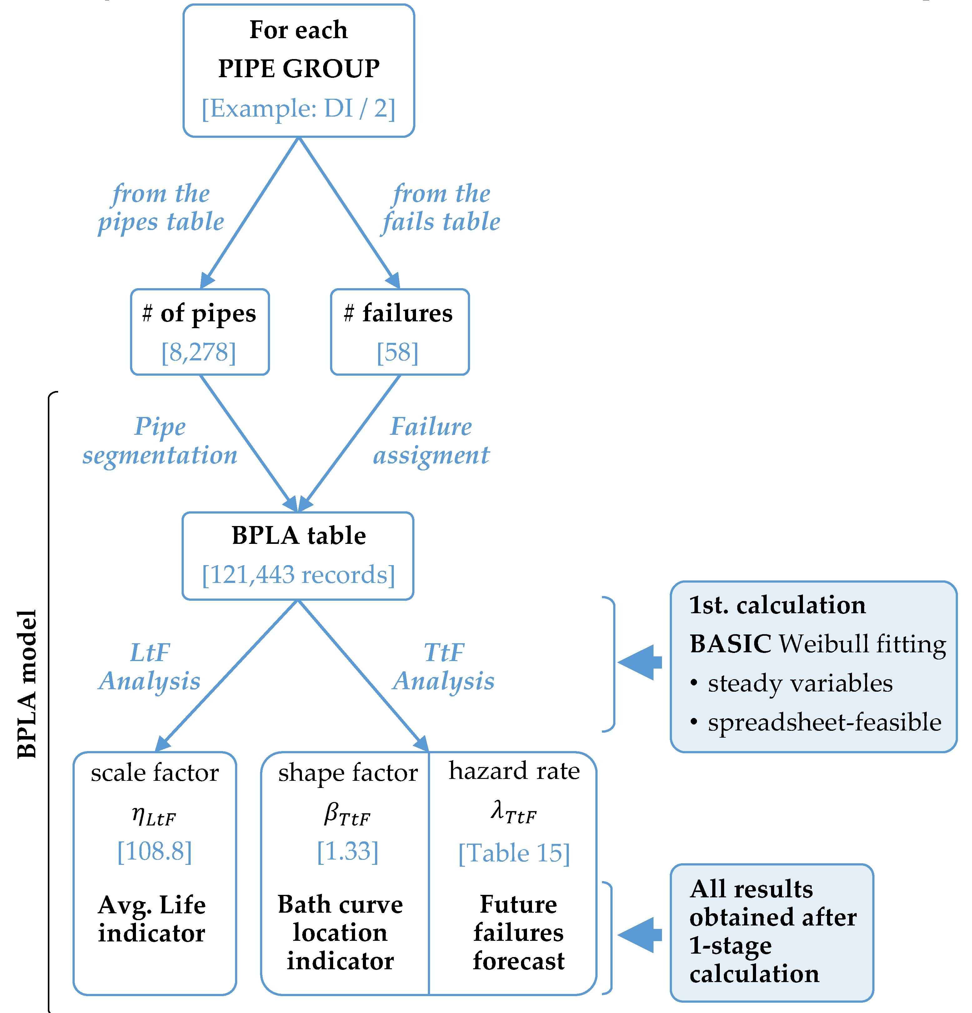
In the field of practical implementation, the BPLA model presents two main advantages compared to other more complex models currently available. The first one is the requirements in terms of software tools and skills of staff. Because of the fact that the calculation employed remains within a standard statistical analysis, those requirements are easily accessible to engineering personnel. The second one is the shortness of the calculation process. Because of the fact that the two time variables used have been independently defined, they can be analyzed at the same time, and therefore all the results of the model are obtained after only one calculation stage.

Figure 9 depicts the whole procedure for the BPLA model. Data sets, calculations performed, results obtained, and also their significance, have been represented in an ordered way. Additionally, the numerical values obtained for one of the pipe groups in the case study have also been included to ease the follow-up of the process. The shadowed boxes highlight the contributions of the model:

The parallel calculations on $\mathrm{LtF}$ and $\mathrm{TtF}$ make it possible to obtain all the results in a single calculation stage.

Standard spreadsheets are suitable for the type of variables to be handled and calculations to be made—though, as mentioned above, in this case, the R software was combined with spreadsheets.

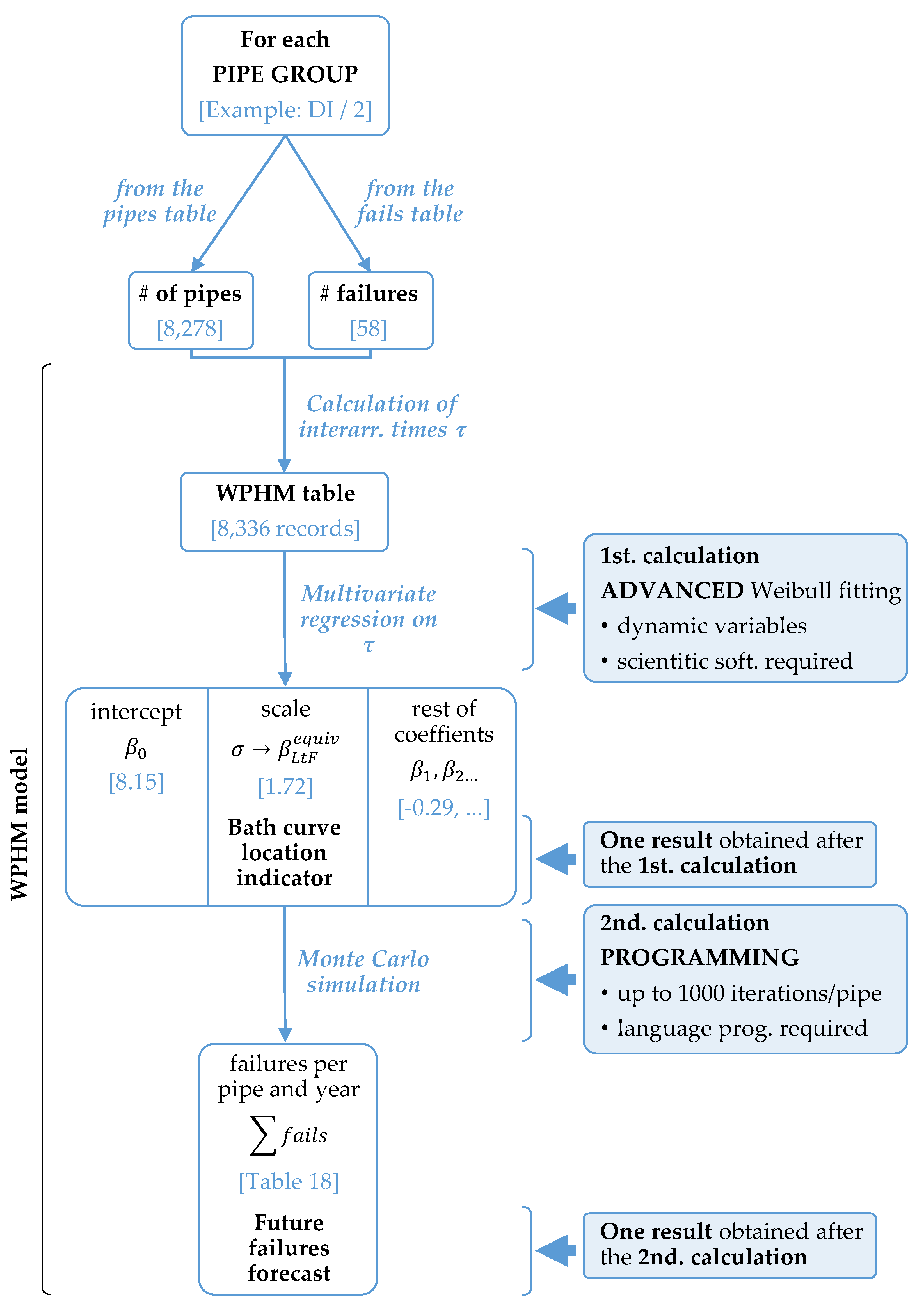
Figure 10 depicts the whole process for the WPHM, under the same criteria followed in Figure 9. In comparison, the shadow boxes show:

• The sequential order of the calculations. This involves performing two stages of calculation to obtain the last result.
• The different nature of the calculations themselves. The first one is a multivariate statistical fitting, for which more than basic software is required—in this case, it has been the R package. The second calculation is a series of simulations (up to 1000 iterations per pipe) for which some sort of programming is needed. In this case, it has been performed through VBA for MSExcel^®.

5. Conclusions

Asset management in general is increasingly becoming more and more relevant in urban water utilities. Their technical, economic and environmental implications are both numerous and significant. In particular, calculating good estimations for service life of pipes is one key piece within the big puzzle of asset management. Several researches have been performed on this issue and, today, several advanced and complex models are already published and tested. The backside of the current state of the art is that it may be inaccessible to many small- and medium-sized water utilities. Their data availability and technical capabilities may not be as high as the ones required by such models.

This paper presents the BPLA model, aimed to get (i) an estimation of the service life of pipes, (ii) an assessment of the pipes failure behavior (bath curve location) and (iii) a forecast for the expected number of failures in the up-coming future. Its novelties are the way the pipe and failures information is processed (by adapting the network data to the maintenance engineering theory and not the other way back), which is combined with the definition of two time variables that are analyzed in parallel. The resulting model calculates all the three mentioned results in a single calculation stage while keeping low requirements on software tools.

A case study has been solved for a utility that supplies water to 500,000 people, with 1000 km pipe network and only two years of available failure records. To apply the model, pipes were classified in homogeneous groups per material (asbestos, ductile iron, cast iron and polyethylene) and diameters. Four representative groups, one per material, were analyzed by the BPLA model and all the results are shown in the case study section. For instance, in the case of pipe group 2 (ductile iron, diameters between 63 and 140 mm, taken as an example in Figure 9 and Figure 10), the estimation of the average service life is nearly 109 years, location on the bath curve is still on the flat intermediate stage and expected future failures will grow from 30 up to 51 in the next five years. As a reference for comparison, the same data sets were also analyzed with the WPHM and the results obtained from both models have been quantitatively contrasted. In average, the relative errors between them were lower than 10–15%, which means a very good accuracy as the complexity of both models are also compared (Figure 9 and Figure 10). In conclusion, such a low errors can be considered fully affordable for the front-line purposes of the BPLA model.

The present research has some novelties over other more complex approximations assessment life models: it presents a less demanding methodology in terms of data and software tools than others currently available, while it allows to get all the results after one single stage of calculation. A compromise between accuracy and simplicity is achieved in this particular case study, considering the consistency of the available data and the possibilities for future improvement, once the model is tuned for next stages.

References

- Shamir, U.; Howard, C.D.D. An Analytic Approach to Scheduling Pipe Replacement. J. AWWA 1979, 5, 248–258. Available online: http://132.68.226.240/urishamir/files/documents/1979%20-%20Shamir%20and%20Howard%20-%20Pipe%20Replacement%20-%20JAWWA.pdf (accessed on 20 January 2020).
- Lauer, W.C. Water Distribution Operator Training Handbook; American Water Works Association: Denver, CO, USA, 2013; ISBN 9781583219546. [Google Scholar]
- Rostum, J. Statistical Modelling of Pipe Failures in Water Networks. Ph.D. Thesis, Norwegian University of Science and Technology, Trondheim, Norway, 2000. [Google Scholar]
- Kleiner, Y.; Nafi, A.; Rajani, B. Planning renewal of water mains while considering deterioration, economies of scale and adjacent infrastructure. Water Sci. Technol. Water Supply 2010, 10, 897–906. [Google Scholar] [CrossRef]
- Fuchs-Hanusch, D.; Kornberger, B.; Friedl, F.; Scheucher, R. Whole of life cost calculations for water supply pipes. Water Asset Manag. Int. 2012, 8, 19–24. [Google Scholar]
- Scholten, L.; Scheidegger, A.; Reichert, P.; Mauer, M.; Lienert, J. Strategic rehabilitation planning of piped water networks using multi-criteria decision analysis. Water Res. 2014, 49, 124–143. [Google Scholar] [CrossRef] [PubMed] [Green Version]
- Amaitik, N.M.; Amaitik, S.M. Prediction of pipe failures in water mains using artificial neural network models. In Proceedings of the International Arab Conference of information Technology (ACIT’2010), Benghazi, Libya, 14–15 December 2010. [Google Scholar]
- Christodoulou, S.; Deligianni, A. A neurofuzzy decision framework for the management of water distribution networks. Water Resour. Manag. 2010, 24, 139–156. [Google Scholar] [CrossRef]
- Kutylowska, M. Neural network approach for failure rate prediction. Eng. Fail. Anal. 2015, 47, 41–48. [Google Scholar] [CrossRef]
- Kabir, G. Planning Repair and Replacement Program for Water Mains: A Bayesian Framework. Ph.D. Thesis, University of British Columbia, Vancouver, BC, Canada, 2016. [Google Scholar]
- Martínez, P.G. Análisis de Variables Explicativas en Modelos de Predicción de Roturas en Redes de Tuberías. Ph.D. Thesis, Universidad Politécnica de Madrid, Madrid, Spain, 2017. Available online: http://oa.upm.es/id/eprint/47857 (accessed on 20 January 2020).
- Motiee, H.; Ghasemnejad, S. Prediction of pipe failure in Tehran water distribution networks by applying regression models. Water Supply 2019, 19, 695–702. [Google Scholar] [CrossRef] [Green Version]
- Di Nardo, A.; Di Natale, M.; Giudicianni, C.; Greco, R. Complex network and fractal theory for the assessment of water distribution network resilience to pipe failures. Water Supply 2018, 18, 767–777. [Google Scholar] [CrossRef]
- Kutylowska, M. Forecasting failure rate of water pipes. Water Supply 2019, 19, 264–273. [Google Scholar] [CrossRef] [Green Version]
- Le Gat, Y.; Eisenbeis, P. Using maintenance records to forecast failures in water networks. Urban Water 2000, 2, 173–181. [Google Scholar] [CrossRef]
- Alvisi, S.; Franchini, M. Comparative analysis of two probabilistic pipe breakage models applied to a real water distribution system. Civ. Eng. Environ. Syst. 2010, 1, 1–22. [Google Scholar] [CrossRef]
- Kimutai, E.; Betrie, G.; Brander, R.; Sadiq, R.; Tesfamariam, S. Comparison of statistical models for predicting pipe failures: Illustrative example with the city of Calgary water main failure. J. Pipeline Syst. Eng. Pract. 2015, 1–2. [Google Scholar] [CrossRef]
- Santos, P.; Amado, C.; Coelho, S.T.; Leitão, J.P. Stochastic data mining tools for pipe blockage failure prediction. Urban Water J. 2017, 14, 343–353. [Google Scholar] [CrossRef]
- Debon, A.; Carrion, A.; Cabrera, E.; Solano, H. Comparing risk of failure models in water supply networks using ROC curves. Reliab. Eng. Syst. Saf. 2010, 95, 43–48. [Google Scholar] [CrossRef]
- Davis, P.; Burn, S.; Moglia, M.; Gould, S. A physical probabilistic model to predict failure rates in buried PVC pipelines. Reliab. Eng. Syst. Saf. 2007, 9, 1258–1266. [Google Scholar] [CrossRef]
- Davis, P.; De Silva, D.; Marlow, D.; Moglia, M.; Gould, S.; Burn, S. Failure prediction and optimal scheduling of replacements in asbestos cement water pipes. J. Water Supply 2008, 4, 239–252. [Google Scholar] [CrossRef]
- Punurai, W.; Davis, P. Prediction of asbestos cement water pipe aging and pipe priorization using monte carlo simulation. Eng. J. 2017, 2, 1–13. [Google Scholar] [CrossRef]
- Yoo, D.; Kang, D.; Jun, H.; Kim, J. Rehabilitation priority determination of water pipes based on hydraulic importance. Water 2014, 6, 3864–3887. [Google Scholar] [CrossRef] [Green Version]
- D’Ercole, M.; Righetti, M.; Raspati, G.S.; Bertola, P.; Ugarelli, R.M. Rehabilitation planning of water distribution network through a reliability-based risk assessment. Water 2018, 10, 277. [Google Scholar] [CrossRef] [Green Version]
- Kleiner, Y.; Rajani, B. Comprehensive review of structural deterioration of water mains: Statistical models. Urban Water 2001, 3, 131–150. [Google Scholar] [CrossRef] [Green Version]
- Rajani, B.; Kleiner, Y. Comprehensive review of structural deterioration of water mains: Physically based models. Urban Water 2001, 3, 151–164. [Google Scholar] [CrossRef] [Green Version]
- Scheidegger, A.; Leitao, J.P.; Sholten, L. Statistical failure models for water distribution pipes–A review from a unified perspective. Water Res. 2015, 83, 237–247. [Google Scholar] [CrossRef]
- van Vossen-van den Berg, J.; van Laarhoven, K.; Hillebrand, B.; Diemel, R. Predicting future failure rates of pipes as a ground for strategic asset management. In Proceedings of the IWA Specialized Conference: LESAM 2019, Vancouver, BC, Canada, 25–27 September 2019. [Google Scholar]
- Azeitona, M.; Vitorino, D.; Marques, J.; Pina, A.; Coelho, S.T. Network failure prediction: Applying statistics to open data and continuous data acquisition. In Proceedings of the Conference: 18° ENASB/18° SILUBESA, Porto, Portugal, 7–9 October 2018. [Google Scholar]
- Yin, T.; Becelaere, T. NETSCAN: The First Step of Dynamic Asset Management; Singapore International Water Week: Singapore, 2018. [Google Scholar]
- Kropp, I.; Baur, R. Integrated failure forecasting model for the strategic rehabilitation planning process. Water Supply 2005, 5, 1–8. [Google Scholar] [CrossRef] [Green Version]
- Ebeling, C.E. An Introduction to Reliability and Maintainability Engineering; Waveland Press: Long Grove, IL, USA, 2019; ISBN-13: 978-1478637349. [Google Scholar]
- Mora, L.A. Mantenimiento, Planeación, Ejecución y Control; Alfaomega Grupo Editor: Ciudad de México, México, 2009; ISBN 13: 9789586827690. [Google Scholar]
- Martins, A.D.C. Stochastic Models for Prediction of Pipe Failures in Water Supply Systems. Master’s Thesis, Instituto Superior Tecnico, Lisboa, Portugal, 2011. [Google Scholar]
- García-Mora, B.; Debón, A.; Santamaría, C.; Carrión, A. Modelling the failure risk for water supply networks with interval-censored data. Reliab. Eng. Syst. Saf. 2015, 144, 311–318. [Google Scholar] [CrossRef]
- Levin, R.I.; Rubin, D.S.; Rastogi, S.; Siddiqui, M.H. Statistics for Management; Pearson: London, UK, 2008; ISBN-13: 978-8177585841. [Google Scholar]
- Ramirez, R. Desarrollo de un Modelo Estadístico para la Estimación de la Vida útil y Predicción de Fallos en Tuberías de agua Potable y su Aplicación en la Gestión de Activos. Master’s Thesis, Universitat Politecnica de Valencia, Valencia, Spain, 2019. [Google Scholar]
- Nwobi, F.N.; Ugomma, C.A. A comparison of methods for the estimation of weibull distribution parameters. Metodološki Zvezki 2014, 11, 65–78. [Google Scholar]
- Lei, Y. Evaluation of three methods for estimating the Weibull distribution parameters of Chinese pine (Pinus tabulaeformis). J. For. Sci. 2008, 12, 566–571. [Google Scholar] [CrossRef] [Green Version]
- Rinne, H. The Weibull Distribution: A Handbook; Chapman & Hall/CRC Press-Taylor & Francis Group: Giessen, Germany, 2009; ISBN-13: 978-1420087437. [Google Scholar]
- Datsiou, K.C.; Overend, M. Weibull parameter estimation and goodness-of-fit for glass strength data. Struct. Saf. 2018, 73, 29–41. [Google Scholar] [CrossRef]
- Therneau, T.M.; Lumley, T. Package survival. Available online: https://cran.r-project.org/web/packages/survival/survival.pdf (accessed on 29 February 2020).
- Christodoulou, S.E. Water network assessment and reliability analysis by use of survival analysis. Water Resour. Manag. 2011, 4, 1229–1238. [Google Scholar] [CrossRef]
Figure 1.
Classification of statistical models for pipe survival analysis (based on Kabir [10]).
Figure 2.
Data requirements for the basic pipes life assessment (BPLA) model.
Figure 3.
Distribution and origin of the pipe data.
Figure 4.
Four pipe examples of the failures modelling approach for BPLA and pre-BPLA models.
Figure 5.
Segmentation and failure assignment to sub-pipes.
Figure 6.
Relation between Weibull’s and parameters [12].
Figure 7.
Main time variables for failure data of one pipe in the WPHM (according to Alvisi and Franchini [16]).
Figure 8.
Empirical and theoretical cumulative distributions after the second analysis.
Figure 9.
Calculation procedure of the BPLA model.
Figure 10.
Calculation procedure of the WPHM.