Quasi-static Flow Model for Predicting the Extreme Values of Air Pocket Pressure in Draining and Filling Operations in Single Water Installations

Abstract

Inertial models have been used by researchers to simulate the draining and filling processes in water pipelines, based on the evolution of the main hydraulic and thermodynamic variables. These models use complex differential equations, which are solved using advanced numerical codes. In this study, a quasi-static flow model is developed to study these operations in hydraulic installations. The quasi-static flow model represents a simplified formulation compared with inertial flow models, in which its numerical resolution is easier because only algebraic equations must be addressed. Experimental measurements of air pocket pressure patterns were conducted in a 4.36 m long single pipeline with an internal diameter of 42 mm. Comparisons between measured and computed air pocket pressure oscillations indicate how the quasi-static flow model can predict extreme values of air pocket pressure for experimental runs, demonstrating the possibility of selecting stiffness and pipe classes in actual pipelines using this model. Two case studies were analysed to determine the behaviour of the quasi-static flow model in large water pipelines.

1. Introduction

The interaction of water columns with entrapped air pockets in water pipelines is difficult to understand because hydraulic and thermodynamic formulations need to be analysed [1,2]. Furthermore, the understanding of water and the air phase is crucial to determine the evolution of involved variables [3].

The water phase can be analysed using flow models depending on fluid and pipe characteristics, where two groups of flow models have been used: (i) inertial models, which consider the fluid inertia, and its resolution is conducted using either the method of characteristics for solving the elastic model (water hammer) [4,5] or numerical methods when the analysis is addressed with a rigid column model (also named the mass oscillation equation) [6,7]; (ii) non-inertial models (or quasi-static flow models), where the fluid inertia is neglected, and its numerical resolution can be computed using a system composed of algebraic equations [1].

The air phase is typically modelled using the polytropic formulation of an entrapped air pocket, where an air pocket can exhibit an adiabatic evolution, isothermal behaviour, or intermediate thermodynamic process [8,9]. An adiabatic evolution is produced when fast manoeuvres of regulating or draining valves are performed in water distributions systems; by contrast, an isothermal evolution is generated for slow manoeuvres [10]. Typically, an intermediate thermodynamic process is considered in actual water pipelines.

Draining and filling operations in water pipelines are typical examples of the interaction of a two-phases flow (water and air), which are periodically performed for operational purposes [4,6]. The analysis of the abovementioned hydraulic events is critical as a filling process is characterised by the rapid compression of an air pocket, which produces pressure surges [4,7], and a draining manoeuvre produces a sub-atmospheric pressure condition owing to the expansion of air pockets [9,11,12]. Both processes should be carefully performed to prevent the risk of water installation collapse. The American Water Works Association [13] provides practical recommendations of water velocity and air pocket pressure to perform these manoeuvres to reduce pipeline collapse.

Recently, draining and filling processes have been investigated using inertial models for the water phase [14,15] and a polytropic law for the air phase [5,8]. Some researchers have used elastic models, where the elasticities of water and pipe have been considered [4,16], and others have used rigid column models to simulate the water phase because the elasticity of air is much higher compared to those of water and pipes [2,7]. Inertial models have been validated in several experimental setups and demonstrated that both models presented a good agreement regarding experimental tests [7,9]. The use of a zero inertia model can avoid the approximation of the Preissman slot for analysing the transition from a free surface to pressurised flow when a fill up occurs in large pipelines [17]. Computational fluid dynamics is an excellent alternative to studying draining and filling manoeuvres in laboratory pipe scale, and its validations has been conducted in draining [11,12] and filling operations [18,19].

This study focuses on the behaviour of draining and filling processes in water pipelines using the quasi-static flow model, which represents a simplified formulation regarding the elastic model and the mass oscillation equation [20,21]. Herein, a simplified mathematical model is presented for computing extreme values of main hydraulic and thermodynamic variables in draining and filling operations in water installations when neither an admitted nor expelled air flow exists for draining and filling operations, respectively [22,23]. The authors neglected the inertial term ($dv/dt=0)$ of the water phase [24,25]; consequently, the quasi-static flow model was obtained. Therefore, the simulation of these operations in water installations was based on three formulations: the quasi-static flow model to represent the water phase [1], the polytropic equation of an entrapped air pocket [26,27], and the piston flow model to simulate air–water interactions [28,29,30]. The numerical resolution of this system is only composed of algebraic equations, which is the main advantage regarding inertial models, where a system composed of algebraic-differential equations must be solved using advanced numerical methods. To verify the mathematical model, an experimental facility was configured at the Laboratory of Fluids at the Polytechnic University of Valencia, Spain, which is composed of a 4.36-m-long (14.3 ft) methacrylate pipeline of internal diameter 42 mm (1.65 inches). Results show that the quasi-static flow model can be used to simulate draining and filling processes in water pipelines, as comparisons between computed and measured extreme values of air pocket pressure indicate their adjustment. Finally, the quasi-static flow model is compared with an inertial model for two case studies (one corresponds to a draining process and the other to a filling operation) to show how extreme values of analysed variables are simulated for the quasi-static flow model.

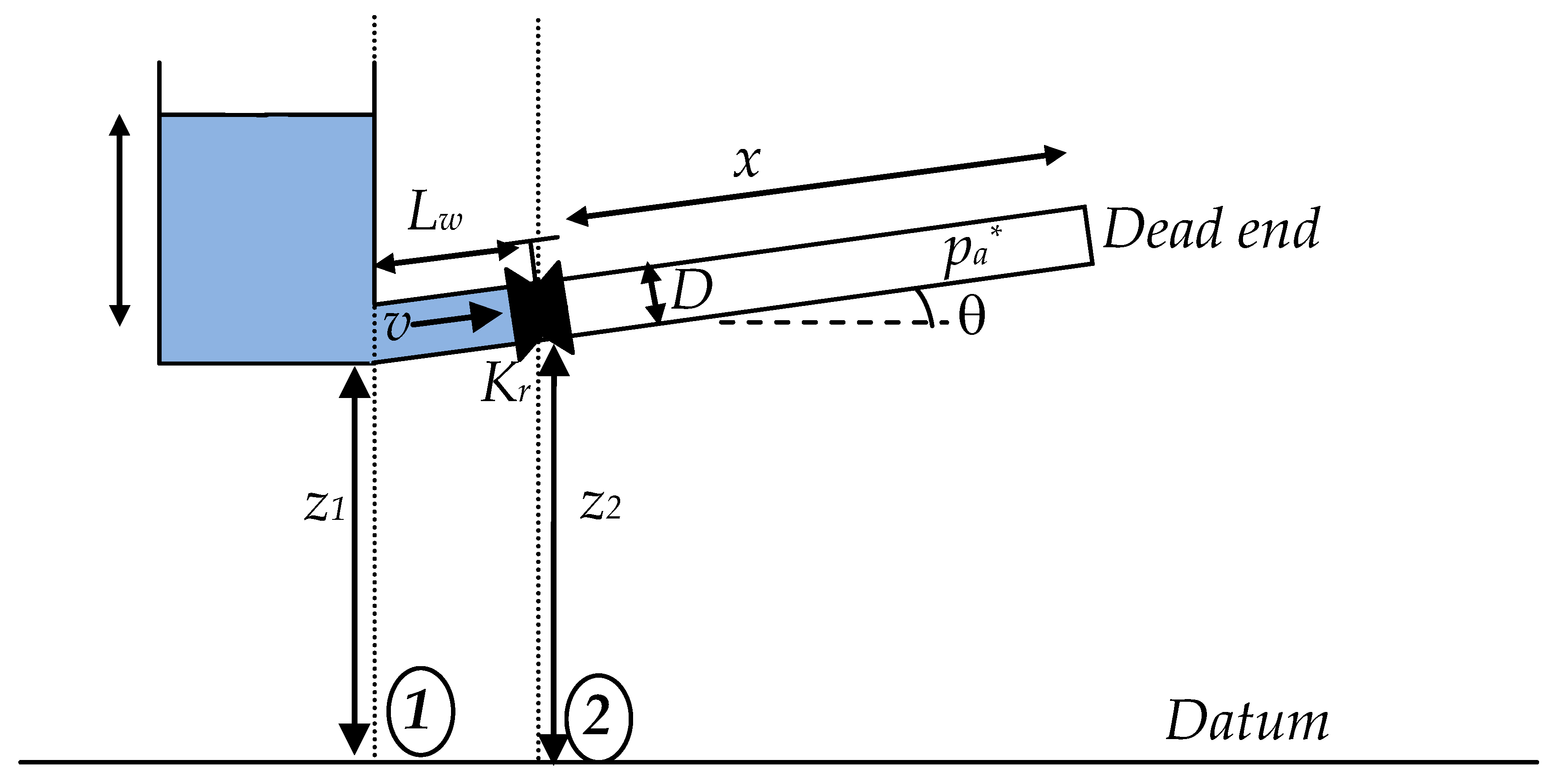
2. Mathematical Model

This section explains the assumptions and formulations to simulate draining and filling operations in single pipelines. The proposed model applies the following assumptions:

• The water column movement is represented by a steady-state equation [1].
• The friction factor (f) is considered constant during transient flow [4,7,8].
• The polytropic model describes the thermodynamic behaviour of the air phase [5,10].
• The air–water interface is simulated using a piston flow model [2,16].

Section 2.1 and Section 2.2 present the mathematical formulations of the draining and filling processes using the quasi-static flow model, respectively.

2.1. Draining Process

The draining process in water pipelines produces sub-atmospheric pressure conditions because the initial air pocket size is expanded during the hydraulic event. Figure 1 illustrates the draining process in a single hydraulic installation, where the main hydraulic and thermodynamic variables are shown. The draining process begins when a drain valve (installed on the downstream end) is opened; subsequently, the water column exits by a drain valve, and an entrapped air pocket increases its initial size. The draining process cannot be concluded based on the opening percentage of the drain valve. This shows that part of the water column remains inside the considered pipeline, and the hydraulic installation should be under a sub-atmospheric condition.

The draining process can be described as follows:

• The steady-state equation.

The mass oscillation equation describes the water column movement during a draining operation, and its formulation for a single pipeline is as follows:

$$\frac{L_w}{g}\frac{dv}{dt}=\frac{p_a^{*}-p_{atm}^{*}}{{\rho }_w{L}_w}+\left(z_1-z_2\right)-\frac{f{L}_w}{2Dg}v\left|v\right|-R_v{A}^{2}v\left|v\right|,$$

(1)

where v = water velocity, t = time, $p_a^{*}=$ air pocket pressure, $p_{atm}^{*}=$ atmospheric pressure, ${\rho }_w=$ water density, $L_w=$ water column size, $z_i=$ pipe elevation at point i, $f=$ friction factor, D = internal pipe diameter, A = cross-sectional area of pipe and R_v = resistance coefficient of a drain valve.

The terms used in the mass oscillation equation are as follows: $dv/dt\left(L_w/g\right)$ is the variation of water velocity over time; $\left(p_a^{*}-p_{atm}^{*}\right)/{\rho }_{w}g$ is the difference in pressure energies between points 1 and 2; $\left(z_1-z_2\right)$ is the difference in potential energies between points 1 and 2; $f{L}_{w}v\left|v\right|/\left(2Dg\right)$ represents the friction losses from points 1 to 2; $R_v{A}^{2}v\left|v\right|$ represents the minor losses in the valve located at point 2.

Neglecting the inertial term (dv/dt = 0) in Equation (1), the steady-state equation (or Bernoulli’s equation) can be expressed mathematically as follows [1]:

$$v_t=\sqrt{\frac{\frac{p_{a,t}^{*}-p_{atm}^{*}}{{\rho }_w{L}_{w,t}}+\frac{\left(z_1-z_2\right)}{L_{w,t}}g}{\frac{f}{2D}+\frac{g{R}_v{A}^2}{L_{w,t}}}}$$

(2)

Equation (2) is used to compute the evolution of water velocity in pipe systems and is categorised as a non-inertial flow. This equation is applicable for slow transient flows.

• The piston flow formulation.

The proposed model considers a perpendicular air–water interface to the main direction of the flow; consequently, it can be applied for water pipelines with a significant slope in their axis. Although real pipelines present a horizontal air–water interface, the considered hypothesis has been implemented by many researchers to obtain a suitable approximation of this phenomenon [1,4,8]. The air–water interface can be modelled as follows [5,16]:

$$\frac{d{L}_w}{dt}=-v,$$

(3)

Applying the finite backward difference approximation, Equation (3) becomes

$$L_{w,t}=L_{w,t-1}-v_t\mathsf{\Delta }t,$$

(4)

where $\mathsf{\Delta }t$ = time step.

Equation (4) describes the evolution of a water column using different time steps.

• The polytropic equation of an air pocket.

The thermodynamic behaviour of an entrapped air pocket can be computed using the following polytropic formulation:

$$p_a^{*}{V}_a^k=p_{a,0}^{*}{V}_{a,0}^k,$$

(5)

where $V_a$ = air volume, k = polytropic coefficient and $t_0=$ time at 0 s (the hydraulic system is at rest).

When the polytrophic coefficient is 1.0, the air pocket exhibits an isothermal thermodynamic behaviour, and the formulation is named as Boyle´s law; if k = 1.4, the air pocket presents an adiabatic evolution [18]. In real water pipelines, intermediate values of the polytropic coefficient can occur between 1.0 and 1.4.

Considering a cross-sectional area of a pipe and an air pocket size ($x_t=L_T-L_{w,t}$), an explicit formulation can be obtained with the involved variables [5]:

$$p_{a,t}^{*}=p_{a,t_0}^{*}{\left[\frac{L_T-L_{w,t_0}}{L_T-L_{w,t}}\right]}^k,$$

(6)

where $L_T$= total length of a pipeline.

2.2. Filling Process

The filling operation is characterised by the compression of an entrapped air pocket, which generates pressure surges. Figure 2 shows all involved variables to describe this process. The operation starts when a regulating valve is opened; subsequently, the pipeline installation begins to be filled by an energy source (pump or tank). As the dead end of a pipeline is closed, an entrapped air pocket is compressed, producing peaks of air pocket pressure.

The filling operation can be described using the following formulations:

• The steady-state equation.

The Bernoulli’s equation is applied to the water column from points 1 to 2 (see Figure 2), which should be considered for emptying operations:

$$v_t=\sqrt{\frac{\frac{p_{1,t}^{*}-p_{a,t}^{*}}{{\rho }_w{L}_{w,t}}+\frac{\left(z_1-z_2\right)}{L_{w,t}}g}{\frac{f}{2D}+\frac{g{R}_r{A}^2}{L_{w,t}}}},$$

(7)

where $p_1^{*}=$ absolute pressure supplied by a pump or tank, and $R_r=$ resistance coefficient of a regulating valve.

• The piston flow formulation.

The air–water interface can be described as follows:

$$L_{w,t}=L_{w,t-1}+v_t\mathsf{\Delta }t,$$

(8)

• The polytropic equation of an air pocket.

Equation (6) can be used to represent the behaviour of an entrapped air pocket during a filling operation.

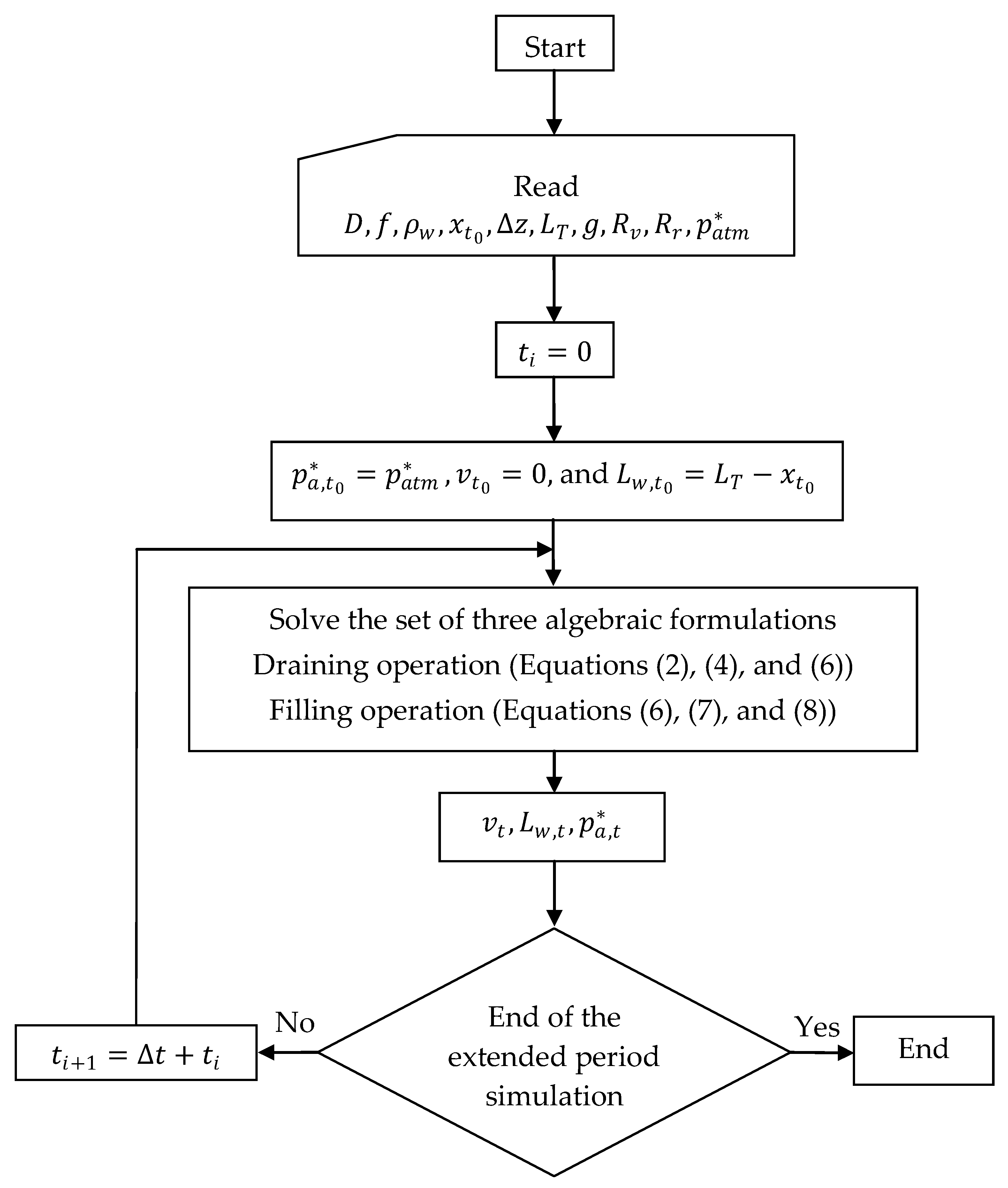
2.3. Numerical Resolution

The resolution of draining processes in single pipelines using the quasi-static model involves the determination of three unknown variables: $L_{w,t},v_t$ and $p_{a,t}^{*}$ for each time step $\left(\mathsf{\Delta }t\right)$. The resolution of the system implies an extended period simulation of single water pipelines. Figure 3 shows the flowchart to solve the set of three algebraic formulations presented in Section 2.1 and Section 2.2 for draining and filling processes, respectively.

The first stage is the reading of water parameters, topographical characteristics of a single pipeline, location of the initial position of the air–water interface and valve coefficients. The pipe slopes were obtained using the formulation, $\sin \theta =\mathsf{\Delta }z/\left(L_T-x_{t_0}\right)$. Next, when the hydraulic system is at rest ($t=0)$, the water velocity is null, and the air pocket pressure is at the atmospheric condition. For the remaining time steps, the three unknown variables are computed by solving Equations (2), (4) and (6) for each time step for a draining process; meanwhile, a filling process can be computed using Equations (6), (7) and (8). At the end of transient phenomena, no changes occur between $t_{i+1}$ and $t_i$ in the estimation of water velocity, air pocket pressure or length of the draining column as the selection of the steady-state model omits the inertial term ($dv/dt=0$).

3. Model Validation

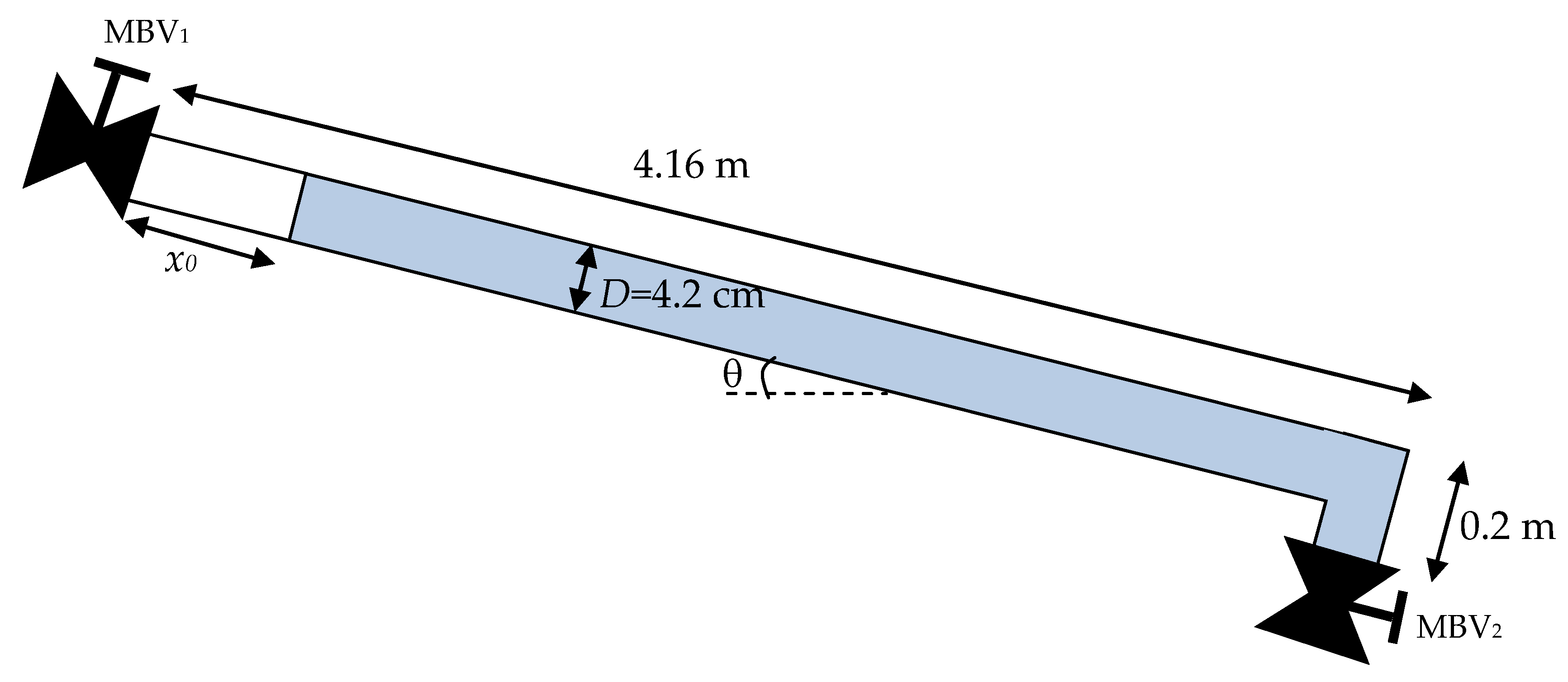
3.1. Experimental Facility

The proposed model was validated for a draining process at an experimental facility located at the Laboratory of Fluids at the Polytechnic University of Valencia, Spain, where a 4.36-m-long (14.3-ft) methacrylate pipeline with an internal diameter of 42 mm (1.65 inches) was used for 12 runs (see Figure 4). A manual ball valve (MBV₁) was positioned at the upstream end to fill the pipe installation. A pressure transducer was located at the highest point of the hydraulic installation to record air pocket pressure oscillations. In addition, another manual ball valve (MBV₂) was placed at the downstream end, where the draining operation was performed. During all experiments, air pocket sizes of 0.205 m (0.67 ft), 0.340 m (1.11 ft) and 0.450 m (1.48 ft) were configured in the pipeline, as well as pipe slopes of 0.457 rad and 0.515 rad. Different valve travels in the MBV₂ were performed, which were defined through marks on a parallel white surface with regard to the position of the MBV₂.

Table 1. Characteristics of runs.

Run No.	${\mathit{x}}_0$ (m)	$\mathit{\theta }$ (rad)	${\mathit{R}}_{\mathit{v}}\times {10}^{-6}$ (m/s/m6)
1	0.205	0.457	11.89
2	0.340	0.457	11.89
3	0.450	0.457	11.89
4	0.205	0.457	25.00
5	0.340	0.457	22.68
6	0.450	0.457	30.86
7	0.205	0.515	14.79
8	0.340	0.515	14.79
9	0450	0.515	14.79
10	0.205	0.515	135.21
11	0.340	0.515	138.41
12	0.450	0.515	100.00

shows the characteristics of all performed runs, which have been previously discussed by the authors [9].

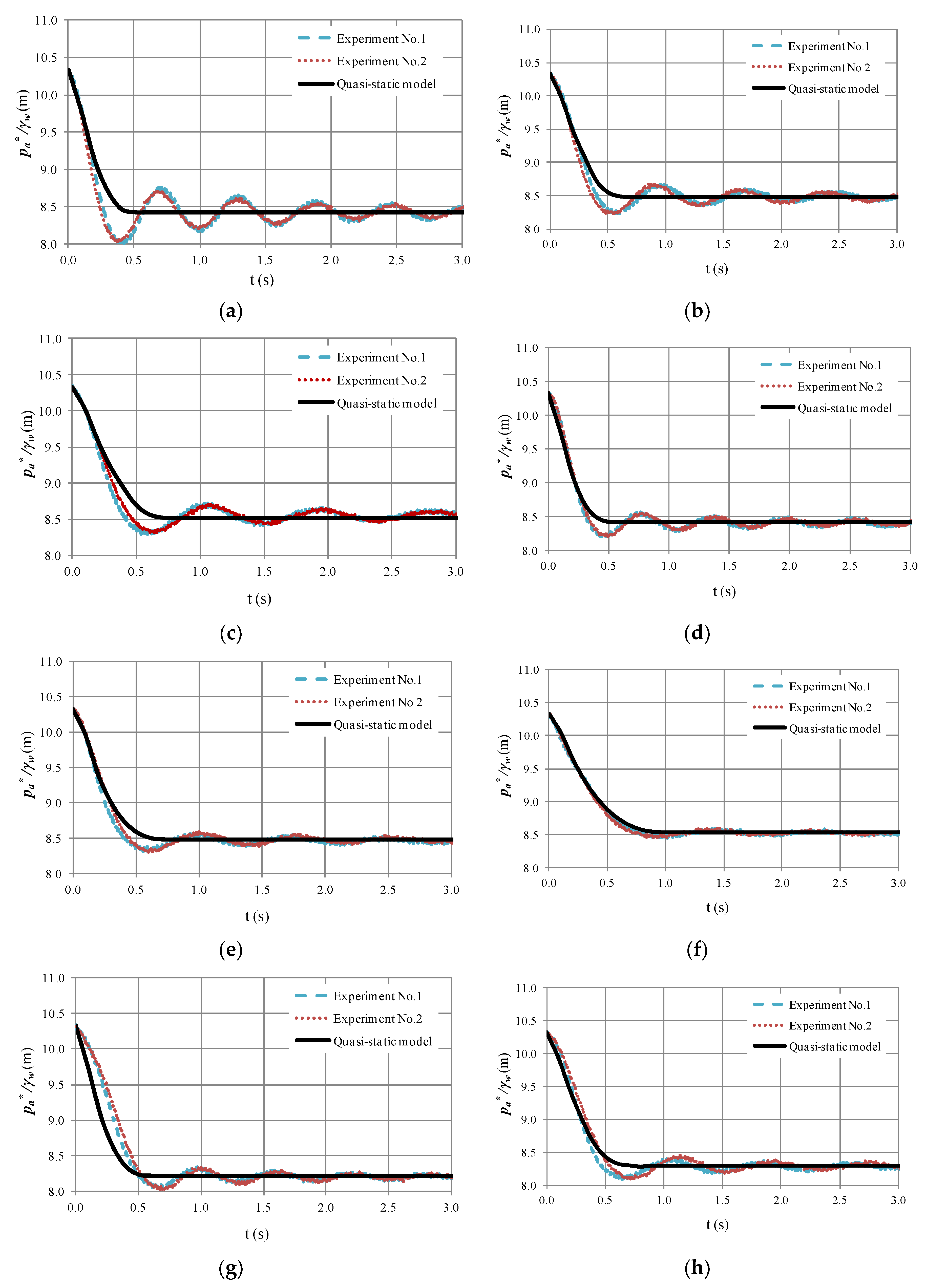
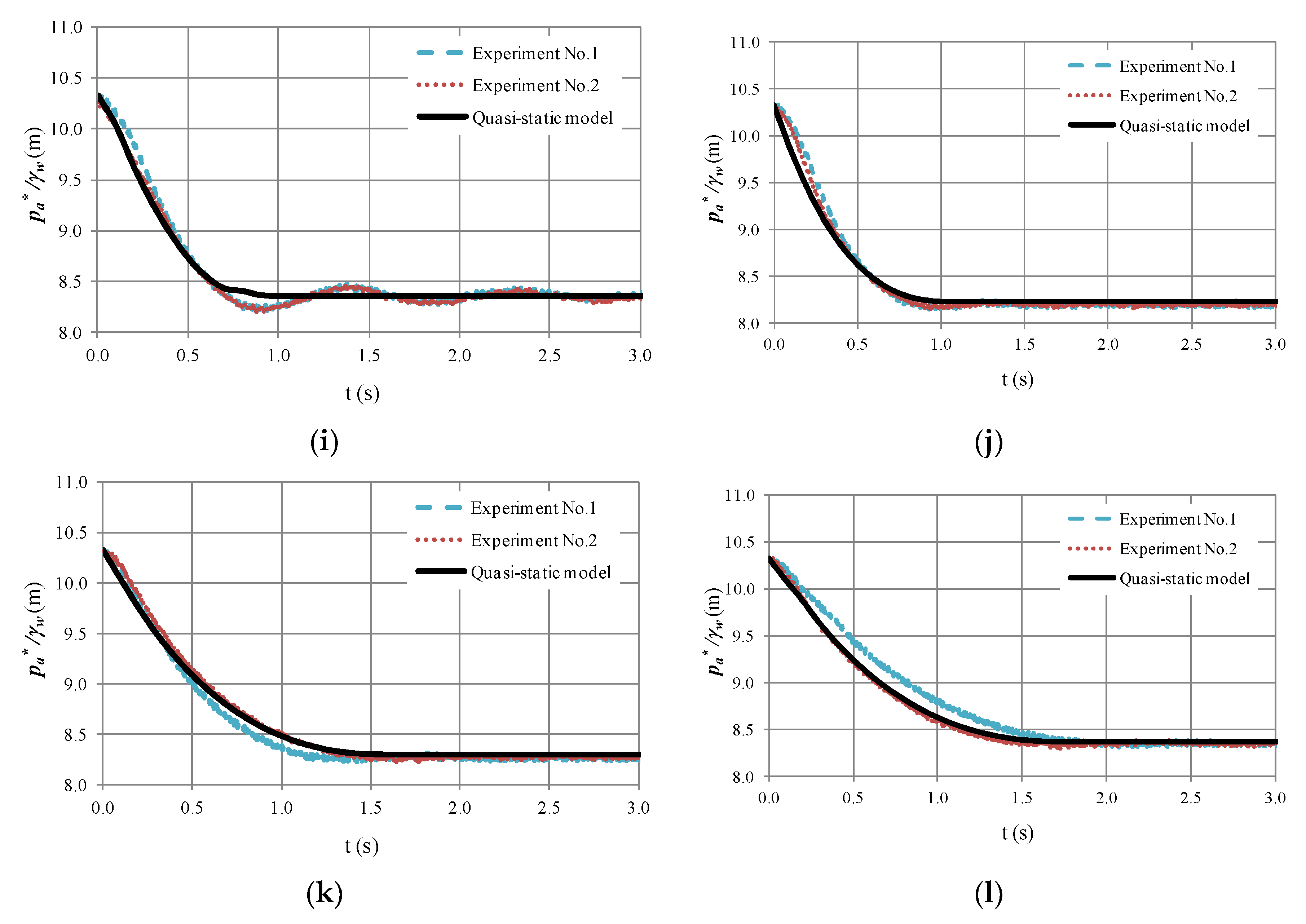
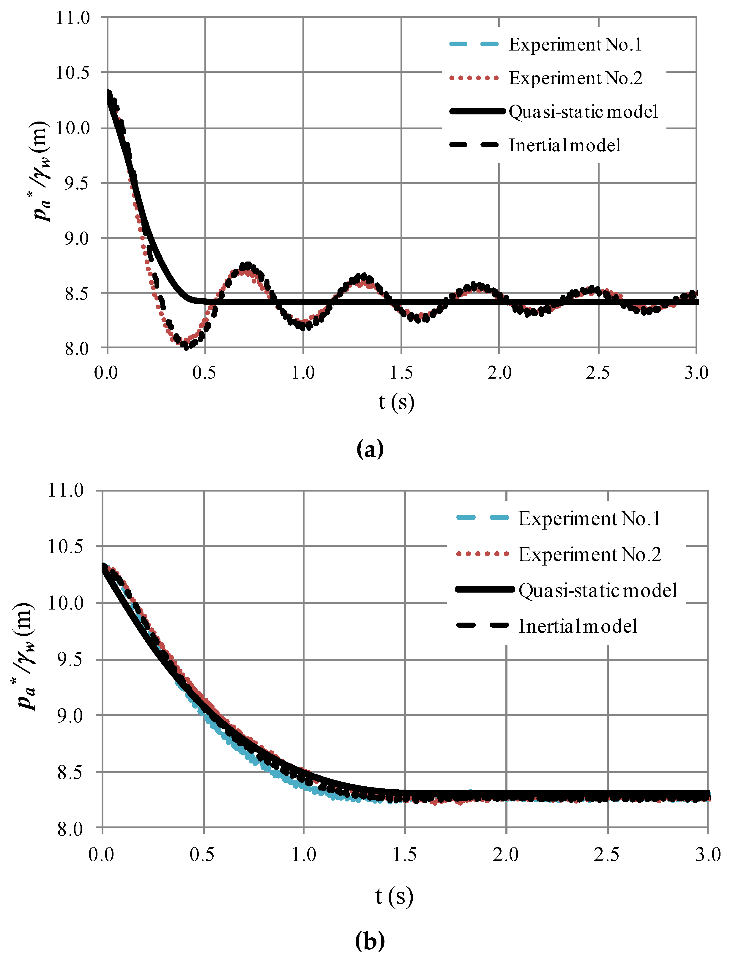
3.2. Model Validation

This section presents a comparison between computed and measured air pocket pressure patterns for 12 runs, as shown in Figure 5. The analysed pipeline installation was composed of an inclined and a vertical pipe branch measuring 4.16 m (13.65 ft) and 0.2 m (0.66 ft), respectively. For all runs, the water column remained inside the inclined pipe branch. The gravity term $\left(z_1-z_2\right)/L_{w,t}$ (see Equation (2)) can be calculated as follows:

$$\frac{z_1-z_2}{L_{w,t}}=\frac{L_T-0.2 \mathrm{m}}{L_T-x_t}\sin \theta +\frac{0.2 \mathrm{m}}{L_T-x_t}\cos \theta ,$$

(9)

During the 12 runs, a constant friction factor (f) of 0.018 and a permanent polytropic coefficient (k) of 1.4 (adiabatic condition) were obtained based on experimental results, as mentioned in a previous publication by the authors [9], as the hydraulic event occurred rapidly.

The quasi-static model is suitable for representing Run 6 and Runs 10 to 12, as presented in Figure 5, where the trends of the experimental results exhibit no oscillations for the highest values of resistance coefficient in MBV2; however, it is not appropriate for simulating air pocket pressure oscillations from Runs 1 to 5 and Runs 7 to 9, where low values of resistance coefficient of MBV2 exist. The quasi-static model cannot simulate these absolute pressure oscillations as Equation (2) neglects the inertial term (dv/dt = 0).

Typically, engineers size a drain valve orifice between 1/3 and 1/4 of an internal pipe diameter in actual pipelines [12]. Therefore, the quasi-static flow model can be used to study the behaviour of the main hydraulic and thermodynamic variables during a draining operation because low values of flow factor in drain valves are obtained in real hydraulic installations.

For all runs, the quasi-static model can predict the drop of sub-atmospheric pressure patterns, which is critical because the minimum sub-atmospheric pressure is required for selecting a stiffness class pipe. For instance, for Run No. 1, the minimum value recorded by the pressure transducer of an absolute pressure head was 8.03 m, and using the quasi-static flow model, a value of 8.42 m was obtained; by contrast, for Run No. 12, a sub-atmospheric pressure head of 8.30 m was obtained, which was close to that of the quasi-static model (8.36 m).

A comparison between the inertial model developed by the authors [6,9] and the quasi-static model is shown in Figure 6 for Runs 1 and 11, which are two representative experimental tests. The remaining tests exhibit similar air pocket pressure patterns. The comparison indicates that the inertial model can accurately predict air pocket pressure patterns for all runs as it considers the inertial term $\left(dv/dt\ne 0\right)$. In Run No. 1, the inertial model predicts not only the drop of the sub-atmospheric pressure head (8.03 m), but also the absolute pressure pattern. Run No. 11 was predicted using both the inertial and quasi-static flow models.

The mean square error (MSE) of the minimum air pocket pressure head for the 12 runs was analysed. Using the quasi-static model, the MSE was 2.494%, implying a good estimation of extreme conditions. As expected, the inertial model agrees well with the calculations of air pocket pressure head oscillations (0.402%) compared with the quasi-static model. Although the inertial model could predict the behaviour of sub-atmospheric pressure patterns more accurately, both models provided good results in terms of extreme values, which enables a stiffness pipe class to be selected using both models.

4. Case Studies

This section presents two case studies regarding draining and filling operations in water distribution systems, which are also used to validate the quasi-static flow model.

4.1. Draining Process

The simulation of a large draining process in a single pipe was performed using the following parameters: L_T = 600 m, D = 0.35 m, k = 1.2, f = 0.018, Δz/L_w,t = sin θ = 0.025 m/m, R_v = 0.06 m/s/m⁶ and t = 10 s. The initial conditions were described by the following parameters: x₀ = 200 m, v(0) = 0 m/s and $p_a^{*}=p_{atm}^{*}$= 101,325 Pa. Figure 7 presents the results of water column length, water velocity and air pocket pressure.

The behaviours of the draining process using the quasi-static flow model are summarised as follows:

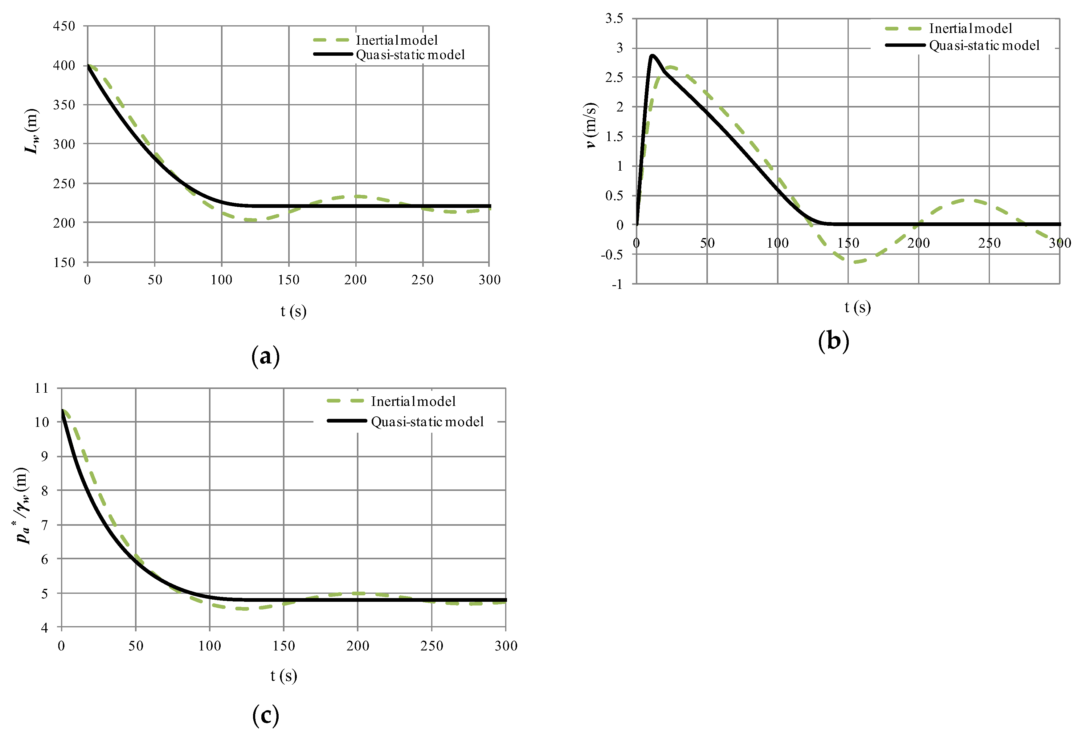
• The quasi-static model can predict the evolution of the water column length during the draining process, as shown in Figure 7a. The quasi-static and inertial models show how part of the water column remains inside of the analysed single pipeline with a mean value of 221.2 m (725.7 ft), where the end of the hydraulic event is presented.
• Figure 7b presents the evolution of water velocity. The maximum water velocity using the quasi-static model is 2.71 m/s (8.89 ft/s) at 15 s, while the inertial model presents a maximum value of 2.63 m/s (8.63 ft/s) at 19.9 s. The quasi-static model cannot reproduce negative velocities.
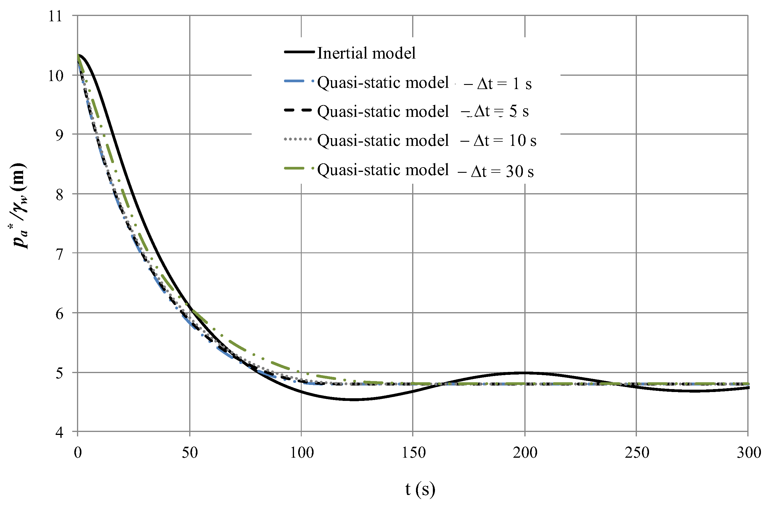
• Regarding the air pocket pressure head (see Figure 7c), the quasi-static model can predict the minimum drop in the sub-atmospheric pressure head of 4.80 m (15.75 ft), which is critical to select the pipe stiffness class. In this hydraulic system, the air pocket pressure head value of 4.80 m (15.75 ft) remains constant from 130 s to the end of the hydraulic event.

Finally, the selection of time step (Δt) is considered. Figure 8 presents the effects of using 1, 5, 10 and 30 s on the behaviour of air pocket pressure patterns. Results show that the quasi-static model exhibits no relevant changes on the behaviour of the absolute pressure pattern when the time step is varied.

4.2. Filling Process

A rapid filling process was simulated using the quasi-static flow model with the following parameters: L_T = 600 m, D = 0.30 m, k = 1.2, f = 0.018, Δz/L_w,t = sin θ = 0.020 m/m, R_r = 0.11 m/s/m⁶ and t = 10 s. The initial conditions were x₀ = 500 m (1640.2 ft), v(0) = 0 m/s (0 ft/s), and $p_a^{*}=p_{atm}^{*}$= 101,325 Pa. Figure 9 shows a comparison between the quasi-static and inertial models [7] of the main hydraulic and thermodynamic variables.

The following can be deduced regarding filling based on the results shown in Figure 9:

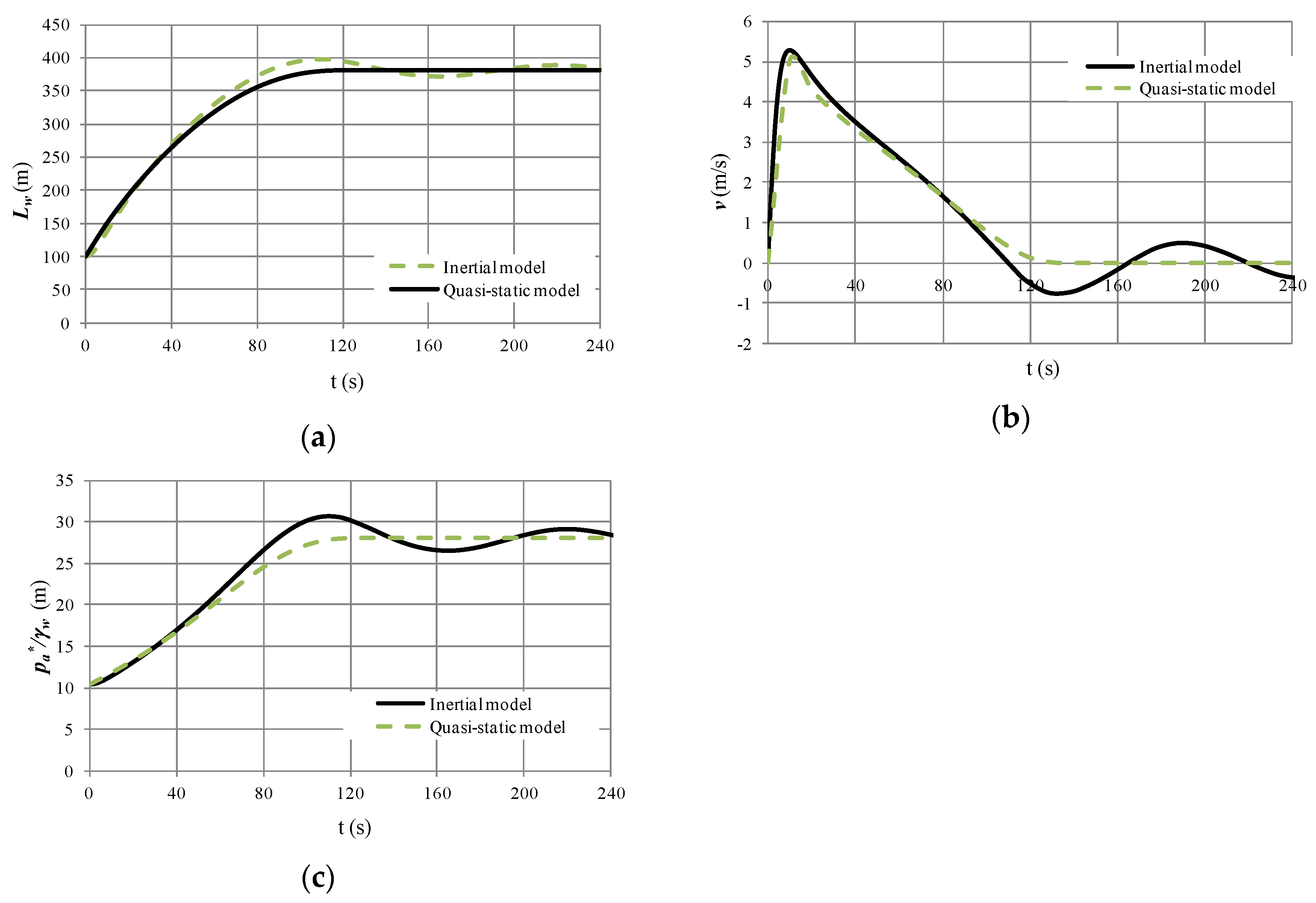
• The quasi-static model is not suitable for predicting oscillation patterns of water column position, water velocity, and air pocket pressure because it neglects the internal term (dv/dt = 0); however, extreme values can be predicted by the quasi-static model, which are used to select the pipe class.
• The quasi-static flow and inertial models can predict the final position of the air–water interface; as shown in Figure 9a, the water column approaches 382 m (1253.3 ft) from 120 s to the end of the hydraulic event.
• The peak of water velocity is predicted by the quasi-static model with a value of 5.03 m/s (16.5 ft/s) at 10 s (see Figure 9b); however, water velocity oscillations from 120 to 240 s are not detected by the proposed model. In this range, the quasi-static model reaches a value of 0 m/s (0 ft/s), while the inertial model presents some oscillations between −0.73 m/s (2.40 ft/s) and 0.50 m/s (1.64 ft/s).
• The more important variable during a filling process is the air pocket pressure. The quasi-static model reaches a maximum value of the absolute pressure head of 28.04 m (91.99 ft/s) at 107 s (see Figure 9c), while the inertial model presents a peak value of 30.7 m (100.72 ft). Subsequently, a difference in the maximum air pocket pressure of 2.66 m (8.73 ft) is presented by comparing these models.

Finally, the effect of time step (Δt) is analysed considering values of 1, 5, 10 and 30 s in the evolution of the air pocket pressure, as shown in Figure 10. A lower time step yields a better prediction of air pocket pressure.

5. Conclusions

In this study, a new one-dimensional mathematical model was developed to compute the main hydraulic and thermodynamic variables during draining and filling processes with an entrapped air pocket in water installations, which was based on the quasi-static flow model, the polytropic formulation of an air pocket and the piston flow model to represent the air–water interface.

The quasi-static model represents an alternative formulation, which can be used by engineers to model filling and draining operations in water single installations, as it can adequately predict extreme values of air pocket pressure patterns. The quasi-static model can be programmed using typical applications (e.g., Microsoft Excel) because complex equations such as the elastic water model or mass oscillation equation are not necessitated, as they are replaced by Bernoulli’s equation. Consequently, the numerical resolution of the proposed model is much easier to use compared with inertial models.

The mathematical model was validated in an experimental facility housing a 4.36-m-long (14.3-ft) methacrylate pipeline with an internal pipe diameter of 42 mm (1.65 inches). Results indicated that the proposed model was suitable for predicting the drop in air pocket pressure patterns in a draining process, which was critical as this extreme value was used to select pipeline characteristics. The minimum drop in sub-atmospheric pressure of the proposed model was compared with the attained values of the inertial model (rigid water column model), in which MSE values of 2.494% and 0.402% were obtained, respectively. The validation of a filling process was not conducted in the experimental facility as these formulations could be applied similarly as a draining process.

Finally, the behaviour of the inertial and proposed models was compared using two cases studies of large diameter (0.35 m or 1.15 ft) for filling and draining operations. The quasi-static model yielded similar results of extreme values of air pocket pressure oscillations compared with the inertial model. The time step did not significantly affect the extreme values of air pocket pressure in the proposed model. Therefore, in a design stage, engineers can apply the quasi-static model to select a stiffness pipe and a class pipe for draining and filling processes, respectively, in water single installations.

The next step is to apply the quasi-static model for complex water pipeline systems.

References

1. Abreu, J.; Cabrera, E.; Izquierdo, J.; García-Serra, J. Flow Modeling in Pressurized Systems Revisited. J. Hydraul. Eng. 1999, 125, 1154–1169. [Google Scholar] [CrossRef]
2. Izquierdo, J.; Fuertes, V.S.; Cabrera, E.; Iglesias, P.; García-Serra, J. Pipeline Start-Up with Entrapped Air. J. Hydraul. Res. 1999, 37, 579–590. [Google Scholar] [CrossRef]
3. Simpson, A.R.; Wylie, E.B. Large Water-Hammer Pressures for Column Separation in Pipelines. J. Hydraul. Eng. 1991, 117, 1310–1316. [Google Scholar] [CrossRef] [Green Version]
4. Zhou, L.; Liu, D.; Karney, B. Phenomenon of White Mist in Pipeline Rapidly Filling with Water with Entrapped Air Pocket. J. Hydraul. Eng. 2013, 139, 1041–1051. [Google Scholar] [CrossRef]
5. Zhou, L.; Liu, D. Experimental Investigation of Entrapped Air Pocket in a Partially Full Water Pipe. J. Hydraul. Res. 2013, 51, 469–474. [Google Scholar] [CrossRef]
6. Coronado-Hernández, O.E.; Fuertes-Miquel, V.S.; Besharat, M.; Ramos, H.M. Experimental and Numerical Analysis of a Water Emptying Pipeline Using Different Air Valves. Water 2017, 9, 98. [Google Scholar] [CrossRef]
7. Coronado-Hernández, O.E.; Besharat, M.; Fuertes-Miquel, V.S.; Ramos, H.M. Effect of a Commercial Air Valve on the Rapid Filling of a Single Pipeline: A Numerical and Experimental Analysis. Water 2019, 11, 1814. [Google Scholar] [CrossRef] [Green Version]
8. Vasconcelos, J.G.; Wright, S.J. Rapid Flow Startup in Filled Horizontal Pipelines. J. Hydraul. Eng. 2008, 134, 984–992. [Google Scholar] [CrossRef] [Green Version]
9. Fuertes-Miquel, V.S.; Coronado-Hernández, O.E.; Iglesias-Rey, P.L.; Mora-Melia, D. Transient Phenomena during the Emptying Process of a Single Pipe with Water-Air Interaction. J. Hydraul. Res. 2019, 57, 1–9. [Google Scholar] [CrossRef]
10. Fuertes-Miquel, V.S.; Coronado-Hernández, O.E.; Mora-Melia, D.; Iglesias-Rey, P.L. Hydraulic Modeling during Filling and Emptying Processes in Pressurized Pipelines: A Literature Review. Urban Water J. 2019, 16, 299–311. [Google Scholar] [CrossRef]
11. Besharat, M.; Coronado-Hernández, O.E.; Fuertes-Miquel, V.S.; Viseu, M.T.; Ramos, H.M. Backflow Air and Pressure Analysis in Emptying Pipeline Containing Entrapped Air Pocket. Urban Water J. 2018, 15, 769–779. [Google Scholar] [CrossRef]
12. Besharat, M.; Coronado-Hernández, O.E.; Fuertes-Miquel, V.S.; Viseu, M.T.; Ramos, H.M. Computational Fluid Dynamics for Sub-Atmospheric Pressure Analysis in Pipe Drainage. J. Hydraul. Res. 2019, 1–13. [Google Scholar] [CrossRef]
13. American Water Works Association (AWWA). Manual of Water Supply Practices -M51: Air-Release, Air-Vacuum, and Combination Air Valves; American Water Works Association: Denver, CO, USA, 2001. [Google Scholar]
14. Laanearu, J.; Annus, I.; Koppel, T.; Bergant, A.; Vučkovič, S.; Hou, Q.; van’t Westende, J.M.C. Emptying of Large-Scale Pipeline by Pressurized Air. J. Hydraul. Eng. 2012, 138, 1090–1100. [Google Scholar] [CrossRef] [Green Version]
15. Tijsseling, A.; Hou, Q.; Bozkus, Z.; Laanearu, J. Improved One-Dimensional Models for Rapid Emptying and Filling of Pipelines. J. Press. Vessel Technol. 2016, 138, 031301. [Google Scholar] [CrossRef] [Green Version]
16. Malekpour, A.; Karney, B.; Nault, J. Physical Understanding of Sudden Pressurization of Pipe Systems with Entrapped Air: Energy Auditing Approach. J. Hydraul. Eng. 2015, 142, 04015044. [Google Scholar] [CrossRef] [Green Version]
17. Noto, L.; Tucciarelli, T. Dora Algorithm for Network Flow Models with Improved Stability and Convergence Properties. J. Hydraul. Eng. 2001, 127, 380–391. [Google Scholar] [CrossRef]
18. Zhou, L.; Liu, D.; Ou, C. Simulation of Flow Transients in a Water Filling Pipe Containing Entrapped Air Pocket with VOF Model. Eng. Appl. Comput. Fluid Mech. 2011, 5, 127–140. [Google Scholar] [CrossRef] [Green Version]
19. Saemi, S.; Raisee, M.; Cervantes, M.J.; Nourbakhsh, A. Computation of Two- and Three-Dimensional Water Hammer Flows. J. Hydraul. Res. 2019, 57, 386–404. [Google Scholar] [CrossRef]
20. Chaudhry, M.H. Applied Hydraulic Transients, 3rd ed.; Springer: New York, NY, USA, 2014. [Google Scholar]
21. Wylie, E.; Streeter, V. Fluid Transients in Systems; Prentice Hall: Englewood Cliffs, NJ, USA, 1993. [Google Scholar]
22. Apollonio, C.; Balacco, G.; Fontana, N.; Giugni, M.; Marini, G.; Piccinni, A.F. Hydraulic Transients Caused by Air Expulsion during Rapid Filling of Undulating Pipelines. Water 2016, 8, 25. [Google Scholar] [CrossRef] [Green Version]
23. Coronado-Hernández, O.E.; Fuertes-Miquel, V.S.; Besharat, M.; Ramos, H.M. A Parametric Sensitivity Analysis of Numerically Modelled Piston-Type Filling and Emptying of an Inclined Pipeline with an Air Valve. In Proceedings of the 13th International Conference on Pressure Surges, Bordeaux, France, 14–16 November 2018; BHR Group: Bordeaux, France, 2018. [Google Scholar]
24. Wang, L.; Wang, F.; Karney, B.; Malekpour, A. Numerical Investigation of Rapid Filling in Bypass Pipelines. J. Hydraul. Res. 2017, 55, 647–656. [Google Scholar] [CrossRef]
25. Coronado-Hernández, O.E.; Fuertes-Miquel, V.S.; Besharat, M.; Ramos, H.M. Subatmospheric Pressure in a Water Draining Pipeline with an Air Pocket. Urban Water J. 2018, 15, 346–352. [Google Scholar] [CrossRef]
26. Ramezani, L.; Karney, B.; Malekpour, A. Encouraging Effective Air Management in Water Pipelines: A Critical Review. J. Water Resour. Plan. Manag. 2016, 142. [Google Scholar] [CrossRef] [Green Version]
27. Martins, S.C.; Ramos, H.M.; Almeida, A.B. Conceptual Analogy for Modelling Entrapped Air Action in Hydraulic Systems. J. Hydraul. Res. 2015, 53, 678–686. [Google Scholar] [CrossRef]
28. Zhou, F.; Hicks, M.; Steffler, P.M. Transient Flow in a Rapidly Filling Horizontal Pipe Containing Trapped Air. J. Hydraul. Eng. 2002, 128, 625–634. [Google Scholar] [CrossRef]
29. Martin, C.S. Entrapped Air in Pipelines. In Proceedings of the Second International Conference on Pressure Surges, London, UK, 22–24 September 1976. [Google Scholar]
30. Cabrera, E.; Abreu, J.; Pérez, R.; Vela, A. Influence of Liquid Length Variation in Hydraulic Transients. J. Hydraul. Res. 1992, 118, 1639–1650. [Google Scholar] [CrossRef]
Figure 1. Schematics of a draining process in a single pipeline with an entrapped air pocket.
Water 12 00664 g001
Figure 2. Schematic of a filling process in a single pipeline with an entrapped air pocket.
Water 12 00664 g002
Figure 3. Flowchart of numerical resolution of a draining process using a quasi-static flow model.
Water 12 00664 g003
Figure 4. Used experimental facility.
Water 12 00664 g004
Figure 5. Comparison between computed and measure of air pocket pressure patterns: (a) Run No. 1; (b) Run No. 2; (c) Run No. 3; (d) Run No. 4; (e) Run No. 5; (f) Run No. 6; (g) Run No. 7; (h) Run No. 8; (i) Run No. 9; (j) Run No. 10; (k) Run No. 11; (l) Run No. 12.
Water 12 00664 g005aWater 12 00664 g005b
Figure 6. Comparison of air pocket pressure patterns between the quasi-static flow and inertial models: (a) Run No. 1; (b) Run No. 11.
Water 12 00664 g006
Figure 7. Comparison between the internal and quasi-static models for a draining process: (a) Water column evolution; (b) Behaviour of water velocity; (c) Air pocket pressure oscillation.
Water 12 00664 g007
Figure 8. Effect of time step during a draining process.
Water 12 00664 g008
Figure 9. Comparison between internal and quasi-static models for a filling process: (a) Water column evolution; (b) Behaviour of water velocity; (c) Air pocket pressure oscillation.
Water 12 00664 g009
Figure 10. Effect of time step during a filling process.
Water 12 00664 g010