Coupling SWAT Model and CMB Method for Modeling of High-Permeability Bedrock Basins Receiving Interbasin Groundwater Flow

Abstract

This paper couples the Soil and Water Assessment Tool (SWAT) model and the chloride mass balance (CMB) method to improve the modeling of streamflow in high-permeability bedrock basins receiving interbasin groundwater flow (IGF). IGF refers to the naturally occurring groundwater flow beneath a topographic divide, which indicates that baseflow simulated by standard hydrological models may be substantially less than its actual magnitude. Identification and quantification of IGF is so difficult that most hydrological models use convenient simplifications to ignore it, leaving us with minimal knowledge of strategies to quantify it. The Castril River basin (CRB) was chosen to show this problematic and to propose the CMB method to assess the magnitude of the IGF contribution to baseflow. In this headwater area, which has null groundwater exploitation, the CMB method shows that yearly IGF hardly varies and represents about 51% of mean yearly baseflow. Based on this external IGF appraisal, simulated streamflow was corrected to obtain a reduction in the percent bias of the SWAT model, from 52.29 to 22.40. Corrected simulated streamflow was used during the SWAT model calibration and validation phases. The Nash–Sutcliffe Efficiency (NSE) coefficient and the logarithmic values of NSE (lnNSE) were used for overall SWAT model performance. For calibration and validation, monthly NSE was 0.77 and 0.80, respectively, whereas daily lnNSE was 0.81 and 0.64, respectively. This methodological framework, which includes initial system conceptualization and a new formulation, provides a reproducible way to deal with similar basins, the baseflow component of which is strongly determined by IGF.

1. Introduction

Hydrological models have become essential tools for water management issues due to their ability to simulate the hydrological cycle through integrated and multidisciplinary approaches, along with their skills to simulate climate change scenarios, land use, and water management [1]. Reliability of such models depends on the spatial and temporal scales covered, as well as the capacity to conceptualize the system functioning [2,3,4]. Those hydrological models operating at a basin scale are powerful decision support tools because they can provide insights into water resource management [5]. Among them, the SWAT (Soil and Water Assessment Tool) model, a physically-based and semi-distributed eco-hydrological open access model [6] stands out. SWAT can simulate the quality and quantity of surface water and groundwater balance components at different catchment scales to predict the impact of climate change on the water balance of large watersheds [7,8] and deduce the effect of human-induced actions on water resources, such as irrigation practices and land-use changes [9]. A recent review of water quality and erosion models reveals that SWAT is, by far, the most used model [10]. However, a downside of SWAT is related to the simplified groundwater concept [11]. The simplified representation of the groundwater discharge and aquifer storage processes has been highlighted by several authors as something that may lead to a misunderstanding of the hydrological processes that occur in groundwater dominated watersheds [12].

One of these limitations is SWAT’s inability to consider interbasin groundwater flow (IGF). IGF can be defined as the naturally occurring groundwater flow beneath the topographic divide that defines the basin boundary introduced in the SWAT model and in other hydrological models. It contributes to the baseflow of another basin different from that from which it was generated [13]. The magnitude of IGF may be especially relevant in high-permeability bedrock areas, such as steep karst areas. IGF maintains permanent streamflow in dry seasons, thus significantly altering the water balance of a region [14]. Despite the fact that IGF is a common hydrological process in large karst areas, it is often difficult to estimate, even tentatively [15]. Methodologies to identify and quantify IGF have traditionally relied on physical techniques, including the soil–water budget and water fluctuation, when there are sufficient data [16,17], tracer techniques measuring mostly environmental chemicals and stable isotope contents of precipitation and stream water [18,19], and groundwater modeling tools for indirect evaluations [20,21]. Some studies have aimed to assess IGF using the SWAT model. More specifically, Palanisamy and Workman (2014) [22] developed the KarstSWAT model to simulate IGF in watersheds dominated by typical karst features, determining input (recharge in sinkholes) and output (discharge in springs) water component dynamics. Malagó et al. (2016) [23] developed the KSWAT model, which was based on a combination of two previous SWAT applications: (1) a SWAT model adaptation to consider fast infiltration through caves and sinkholes up to the deep aquifers developed by Baffaut and Benson (2009) [24] and (2) a karst flow model in Excel to simulate spring flow discharge developed by Nikolaidis et al. (2013) [25]. More recently, Nguyen et al. (2020) [14] proposed a two linear reservoir model to represent the duality of aquifer recharge and discharge processes in a karst-dominated area in Germany. However, this interest is ongoing and, to our knowledge, the SWAT model has yet to be combined with the CMB method to improve hydrological cycle simulation in those basins where there is a difference between groundwater flow divides and surface topographic divides.

The evaluation of IGF is a complex, uncertain task when groundwater system functioning is partially unknown and the spatiotemporal coverage of data is too low to implement suitable evaluation techniques. In general, spatiotemporal coverage of environmental variables decreases in mountainous areas, thereby limiting the range of suitable techniques to assess IGF and other water balance components. In ungauged areas, IGF can be indirectly assessed when enough is known about groundwater system functioning to assert that IGF equals net aquifer recharge, which is the typical circumstance in most mountainous karst areas in a natural regime. In steep basins with gaining streams under a natural (undisturbed) regime, long-term net aquifer recharge (R) and discharge can be equated when groundwater abstraction, direct evapotranspiration from shallow aquifers, and underflow to deep aquifers are virtually null [26,27]. In such undisturbed hydrological functioning, net aquifer discharge equals the baseflow component of streamflow [28,29,30,31], and the problem shrinks to a matter of implementing suitable and viable techniques to determine R. Note that R is the infiltration amount that effectively contributes to the aquifer storage after some delay, smoothing out the variability inherent to precipitation events [32,33]. To assess renewable groundwater resources that finally reach streambeds, R is the governing variable [4,34].

Different methods can be used for R [35,36]. An independent, well-known method to determine R is the atmospheric Chloride Mass Balance (CMB) method [37,38,39,40,41]. The CMB method has been widely applied in different orographic, climatic, and geological contexts to yield mostly long-term (steady) R estimates when recharge water salinity can be attributed to the atmospheric salinity that reaches the water table. The CMB method was recently used to assess distributed mean R from precipitation and its uncertainty over continental Spain by verifying that the CMB variables were steady long-term [34,42]. This data availability was the reason the CMB method was chosen to assess IGF in areas with no human activities. In other territories, other techniques strictly intended for regional R can be selected for IGF evaluations when there are available data sets of similarly sufficient confidence.

This paper aims to evaluate the reliability of coupling the SWAT model and the CMB method to improve the modeling of streamflow in high-permeability bedrock basins receiving IGF. To that end, two main methodological steps are introduced. The first conceptualizes the hydrogeological functioning to confidently estimate IGF from existing CMB datasets for a control period and introduces a new formulation to generate a long-term baseflow series. The second step integrates corrected baseflow series into the SWAT model to improve the streamflow simulation. This methodology has been applied to the Castril River basin (CRB), which is an undisturbed, high-permeability bedrock area, characterized by the strong contribution of IGF to streamflow, as evidenced by a preliminary surface runoff coefficient greater than one.

2. Materials and Methods

2.1. Study Area

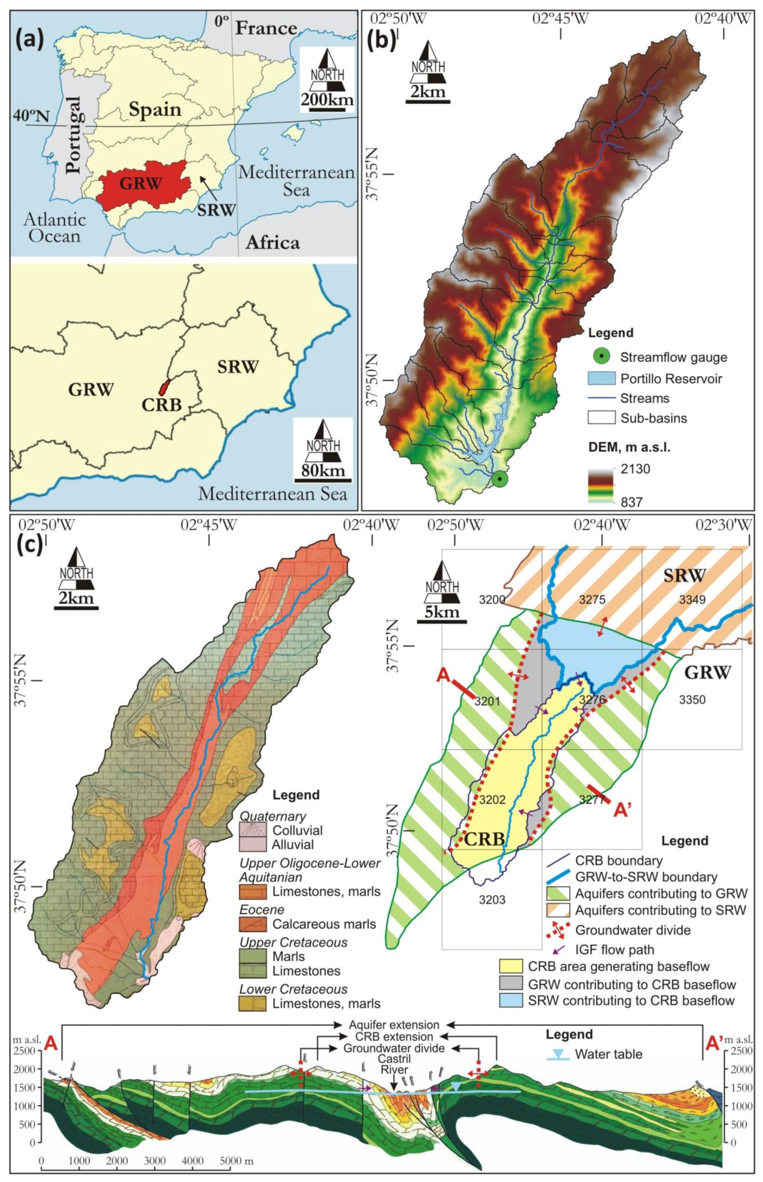
The Castril River is an aquifer-fed mountain stream located 37°47’–37°59’ north and 2°40’–2°50’ west at the headwater of the Guadalquivir River watershed (GRW) in the province of Granada in southern Spain, adjacent to the Segura River watershed (SRW) (Figure 1a). The Castril River basin (CRB) headwater extends from the GRW-SRW divide (peak elevation is 2130 m a.s.l. in the north) to the Portillo Reservoir (outlet is 837 m a.s.l. in the south), covers an area of about 120 km², and flows southward among the Sierra de Castril (west) and Sierra Seca (east) Mountains [43] (Figure 1b).

The climate is comparable to the continental Mediterranean, according to the Köppen classification [44]. Average annual precipitation is about 770 mm, with a coefficient of variation of 0.31 over the period 1951–2017. Precipitation is generated by Atlantic weather fronts coming in from the west and by short, intense Mediterranean convective storms. Most precipitation occurs during the autumn and spring. In winter, wet westerly and cold northerly winds predominate, whilst in summer and autumn, wet easterly and warm southerly winds blow [45]. Based on the period 1951–2016, the average annual temperature is about 8 °C, with the lowest temperatures in January and the highest in August. Average annual potential evapotranspiration is about 800 mm [46].

Geologically, the area belongs to the inner Prebetic domain of the external zone of the Alpine Betic Chain, which includes the following synthetic succession from bottom to top [47,48]: (1) Triassic gypsum-rich marls and clays (Keuper facies) with occasional limestones (Muschelkalk facies); (2) Lower and Middle Jurassic dolomites and oolitic limestones; (3) Upper Jurassic nodule limestones, calcareous marls, and marls; (4) Lower Cretaceous dolomites, dolomitic limestones, and marls; (5) Upper Cretaceous calcareous marls, marls, and dolomitic limestones; and (6) Paleocene to Middle Miocene limestones, marls, and calcarenites [48,49]. Small Late Quaternary alluvial deposits intermittently fill the valleys (Figure 1c).

From a hydrogeological point of view, geological materials can be classified into four groups, attending to the permeability type and storage capacity reported by the Geological Survey of Spain (IGME) (1988, 1995, 2001) [50,51,52]: (1) Triassic marls and clays are low-permeability materials that form the impervious boundary of local aquifers; (2) Jurassic and Cretaceous carbonate materials form highly permeable aquifers as thick as 300 m and have manifest karst features; (3) Jurassic and Cretaceous marls and calcareous marls are low-permeability materials, often confining the above Jurassic and Cretaceous carbonate materials; and (4) Late Quaternary alluvial deposits form temporary unconfined aquifers (Figure 1c).

Hydrogeological functioning of the area was defined by IGME (1988, 1995, 2001) [50,51,52]. Aquifer boundaries, groundwater divides, and groundwater flow paths were established from hydrogeological maps, piezometry, and chemical and isotopic data. These hydrogeological criteria enabled experts to identify preferred areas for aquifer recharge in summits and for aquifer discharge, at the precise place where the incisive valley topography intersects the piezometry of Cretaceous carbonate aquifers to generate intermittent (upstream) and permanent (downstream) springs (Figure 1c). Downstream, outside the study area, Pliocene and Quaternary alluvial formations fill the Castril River valley and form an unconfined aquifer that hydraulically connects to the stream [43].

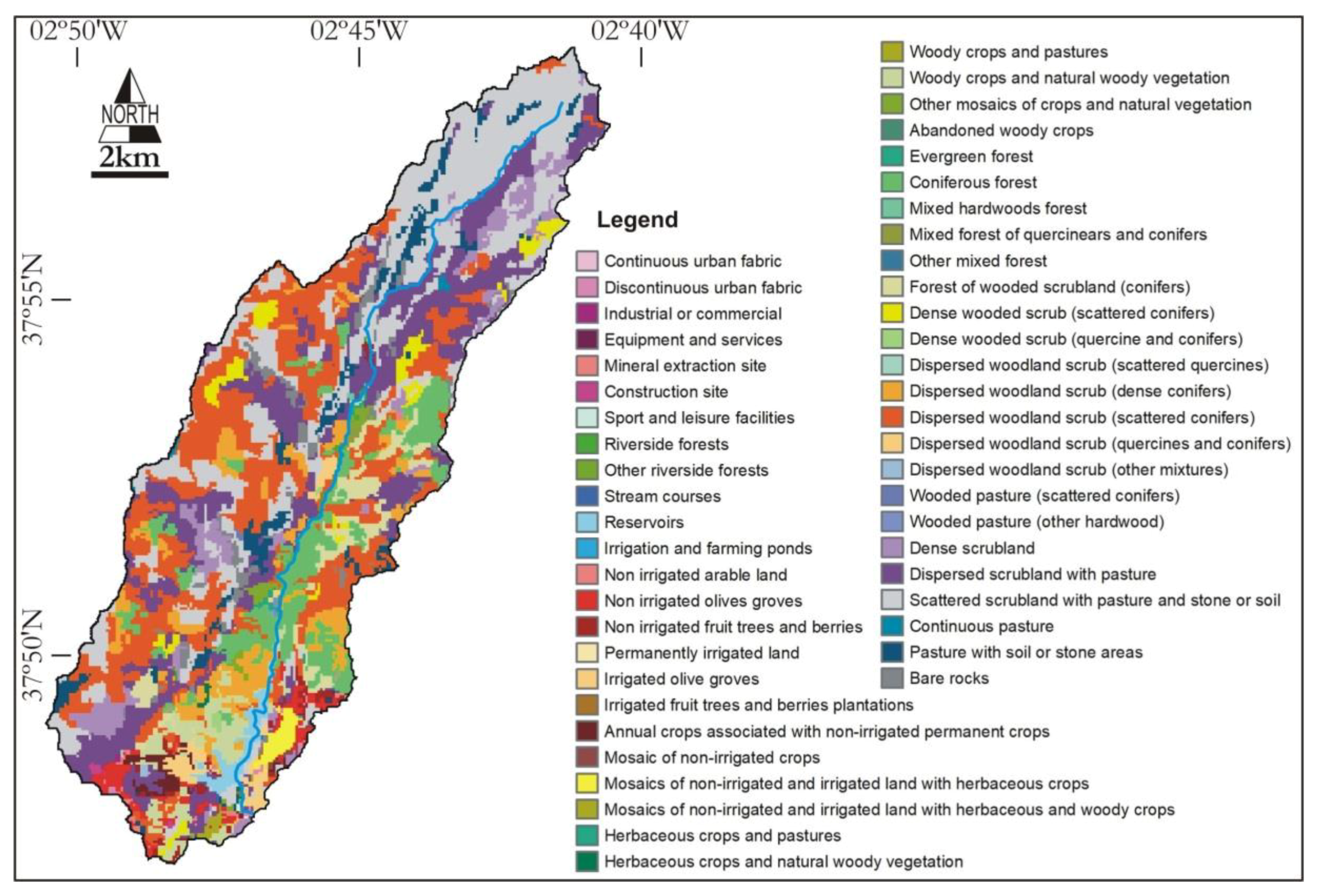
The study area is within the Sierra de Castril Natural Park, which has been an environmentally protected space since 1989, and is catalogued as a zone of special conservation for wildlife by the European Natura 2020 network. With respect to land use, forest, grassland, woodland and shrubland, sparsely vegetated areas, bare areas, and marginal rain-fed crops occupy most of the basin surface (Figure 2). Other marginal uses are seasonal livestock (sheep and goats), irrigated traditional crops, and riverine forest of Pinus nigra and Pinus Halepensis [53]. Neither permanent human settlements nor relevant water uses exist.

2.2. Overall Model Description

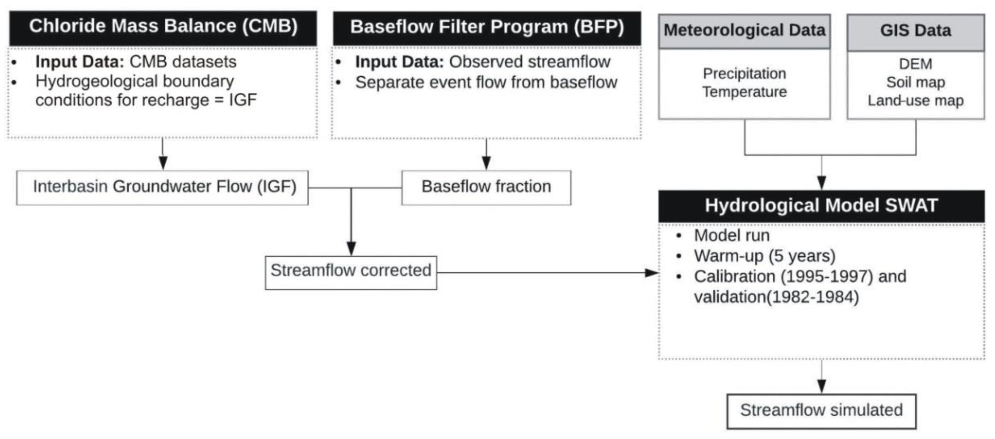
A coupled application of the SWAT model and the CMB method to improve streamflow simulation by considering IGF is introduced. This application includes four steps, shown as bulleted lists (Figure 3). The first step uses the CMB method to assess the magnitude of IGF contributing to the CRB baseflow from another upstream GRW and SRW areas, as described in Section 2.3. The second step uses the automated digital filter program BFLOW to split daily streamflow records into baseflow and surface runoff components, as a prerequisite to correct streamflow records by adding IGF to the baseline component, as described in Section 2.4. The third step uses the SWAT model to compare simulated streamflow with and without IGF, as described in Section 2.5. The fourth step uses the SWAT model for standard calibration and validation of simulated streamflow by considering the IGF correction, as described in Section 2.5.

2.3. CMB Method

2.3.1. CMB Method Application for Aquifer Recharge over Continental Spain

The atmospheric chloride mass balance (CMB) is one of the most widely used methods to estimate net aquifer recharge (R) from precipitation in different orographic, climatic, and geological contexts [35,36]. The CMB is a global method based on the principle of mass conservation of a conservative tracer, in this case the chloride ion, atmospherically contributing to the land surface. This technique yields mostly long-term (steady) R estimations when recharge water salinity can be attributed to the atmospheric salinity that reaches the water table [37,38,39,40,41].

The CMB method was recently applied to estimate distributed spatial mean R and its natural uncertainty (standard deviation) over continental Spain. For a confident application, the long-term steady condition of the CMB variables: atmospheric chloride bulk deposition, chloride export flux by surface runoff, and recharge water chloride content was verified [34,42,54]. This evaluation examined the influence of hydraulic properties (mostly permeability and storability) of different aquifer lithologies on R estimates, as well as the potential contribution of non-atmospheric sources of chloride [55]. For local usage, the reliability and hydrological meaning of distributed R were evaluated by comparing them with local, presumably trustworthy R estimates; one of these local cases was the CRB. Ordinary kriging was used to regionalize the CMB variables at the same 4976 nodes of a 10 km × 10 km grid. In each grid node a mean R value was estimated. Nodal R values were affected by two main types of uncertainty, the natural variability of the CMB variables and the error from its mapping. These uncertainties were identified and estimated [34,42].

The evaluation covered a 10-year period, which represented the critical balance period for the CMB variables to reach comparable steady means and standard deviations. This 10-year period matches the decadal global climatic cycles acting on the Iberian Peninsula, with irregular ~5-year positive and negative phases that follow the North Atlantic Oscillation trend [45,56]. Considering that (1) at least a 10-year balance period is required for reliably steady R evaluations in continental Spain and (2) the CMB datasets preferably spanned the period 1994–2007, the control period (1996–2005), which span a full 10-year long NAO climatic cycle, was chosen to estimate R in this work. Other authors have also implemented these CMB datasets for reliable local R evaluations in different climatic and geological settings, such as Andreu et al. (2011) [27] in Sierra de Gádor karst Massif in Southern Spain, Raposo et al. (2013) [57] in varied geological contexts in Galicia, on the coast of Northern Spain, and Barberá et al. (2018) [58] in the high-mountain, weathered-bedrock Bérchules basin in Southern Spain.

2.3.2. IGF Series Generation

As introduced in Section 1, long-term steady R and IGF can be made equivalent in steep basins with gaining stream under natural (undisturbed) regime when groundwater abstractions, direct evapotranspiration from shallow aquifers, and underflow to deep aquifers are virtually null, and the hydrogeological functioning is well-defined [28,29,30,31]. This is the case of the CRB, as described in Section 2.1, because human water use is virtually null and there is enough hydrogeological information. The fraction of R produced in upstream contributing areas can be used as a reliable proxy for the additional baseflow fraction contributing to the CRB baseline [26,27]. To assess the IGF, R is the significant factor [4,34].

As described above, several cells, each one yielding a nodal mean R value and its standard deviation for the control period (1996–2005) instead of a yearly R series, cover the CRB and upstream contributing areas. Adapted from Pulido-Velázquez et al. (2018) [59], a procedure is introduced to obtain the yearly R series by adopting the temporal structure of the yearly P series for the control period (1996–2005). This model uses a correction function that forces the control R series to have the same relative deviation as the control P series, while maintaining the magnitude of its initial mean and standard deviation. The calibrated function is applied to obtain a yearly R series, presuming the correction function does not change. The calculation includes the following steps:

Average change in mean and standard deviation of P and R for the same control period (1996–2005):

$$\Delta \mathrm{m}=\frac{\mathrm{m}\left(R\right)-\mathrm{m}\left(P\right)}{\mathrm{m}\left(P\right)}$$

(1a)

$$\Delta \sigma =\frac{\sigma \left(R\right)-\sigma \left(P\right)}{\sigma \left(P\right)}$$

(1b)

where $\Delta \mathrm{m}$ is the change in mean and $\Delta \sigma$ is the change in standard deviation.

Normalization of the yearly P series:

$$P{n}_i=\frac{P_i-\overline{P}}{{\sigma }_R}$$

(2)

where P_i is i–year P and Ps_i is its normalized value, $\overline{P}$ is mean P, and ${\sigma }_R$ is standard deviation of mean R.

Generation of yearly R series from yearly P series:

$$R_i={\mathrm{m}}_C+{\sigma }_C·P{s}_i$$

(3)

where R_i is i–year R, and ${\mathrm{m}}_C$ and ${\sigma }_C$ are expressed as:

$${\mathrm{m}}_C=\mathrm{m}\left(P\right)·\left(1+\Delta \mathrm{m}\right)$$

(4a)

$${\sigma }_C=\sigma \left(P\right)·\left(1+\Delta \sigma \right)$$

(4b)

When Equation (4) is applied to the control yearly P series, the generated yearly R series adopts the same mean and standard deviation as the control R series from Alcalá and Custodio (2014, 2015) [34,42]. When this procedure is applied to the full yearly P series, the equivalent yearly R series is obtained by assuming that the bias correction remains invariant over the full observation period.

2.4. BFLOW Program

The automated digital filter program (BFLOW) to split daily streamflow records into the baseflow and surface runoff components was used. Nathan and McMahon (1990) [60] were the first to implement this recursive digital filter technique for baseflow analysis. The hypothesis of BFLOW is that low-frequency signals represent the baseflow component while high-frequency signals represent the runoff component [61]. This technique gives results similar to those obtained using other automated models or manual techniques despite having no physical basis. BFLOW has been used in many studies related to the SWAT model [30,62]; see Arnold and Allen (1999) [63] for more details about this technique. The baseflow obtained by BFLOW was increased by adding IGF, calculated in previous section.

2.5. SWAT Model

2.5.1. Description of the SWAT Model

The Soil and Water Assessment Tool (SWAT) is a long-term watershed hydrological model with strong physical mechanisms, developed jointly in 1994 by the Agricultural Research Service of the United States Department of Agriculture (USDA-ARS) and Texas A&M AgriLife Research, part of the Texas A&M University System. The SWAT model simulation includes atmospheric precipitation, surface runoff, subsurface flow, evapotranspiration, groundwater flow, river network flow concentration, and other intermediate water balance components subjected to variable delays [6]. The SWAT model first divides the study area into several hydrological response units (HRUs) based on the digital elevation model (DEM), land use, soil type, and meteorological data. Then, SWAT establishes a hydrophysical conceptual model of each HRU, calculates runoff in each HRU, and finally connects the entire set of the HRU runoff responses through the river network of the study area toward the basin outlet. The hydrological processes simulated by the SWAT model are based on the following water balance equation:

$${\mathrm{SW}}_{\mathrm{t}}={\mathrm{SW}}_0+{\displaystyle \sum }_{i=1}^t{\left({\mathrm{P}}_{\mathrm{day}}-{\mathrm{E}}_{\mathrm{day}}-{\mathrm{Q}}_{\mathrm{surf}}-{\mathrm{W}}_{\mathrm{seep}}-{\mathrm{Q}}_{\mathrm{gw}}\right)}_i$$

(5)

where ${\mathrm{SW}}_{\mathrm{t}}$ is final soil–water content (mm H₂O), ${\mathrm{SW}}_0$ is initial soil–water content (mm H₂O), t is time (days), ${\mathrm{P}}_{\mathrm{day}}$ is precipitation on day i (mm H₂O), ${\mathrm{ET}}_{\mathrm{day}}$ is evapotranspiration on day i (mm H₂O), ${\mathrm{Q}}_{\mathrm{surf}}$ is surface runoff on day i (mm H₂O), ${\mathrm{W}}_{\mathrm{seep}}$ is water amount that enters the vadose zone from the soil profile on day i (mm H₂O), and ${\mathrm{Q}}_{\mathrm{gw}}$ is groundwater return flow on day i (mm H₂O).

2.5.2. Data, Model Set-Up, Calibration, and Validation

Datasets used to implement the SWAT model were: (1) the 25-m resolution DEM from the Spanish National Geographic Institute (IGN); (2) the land-use map (scale 1:25,000) from the Andalusian Environmental Information Network (REDIAM); (3) the 1-km resolution georeferenced soil data from the World Soil Coordination Map; (4) the 5-km resolution nodal daily precipitation series in Spain from the Spanish National Weather Service (AEMET) grid version 1.0, which cover the period 1951–2017; (5) the 10-km resolution nodal daily temperature series in Spain from the fifth version of the high-resolution SPAIN02 grid, which cover the period 1951–2016; and (6) the 24-h streamflow records downloaded from the Spanish Centre for Public Works Studies and Experimentation (CEDEX) website. The open source QGIS interface for SWAT (QSWAT 1.8) was used to set up the SWAT model.

The SUFI-2 algorithm of SWAT-CUP (Calibration and Uncertainty Programs) to calibrate and validate the SWAT model was used. Based on our previous modeling experiences [64,65], twenty-one widely used flow calibration parameters and their ranges were initially selected. Aimed at reaching an acceptable calibration, two iterations (representing 500 simulations each) were performed; the first included 13 parameters on a monthly scale, the latter included 8 parameters on a daily scale. To mitigate the effect of initial soil–water condition, a five-year warm-up period was imposed [66]. The periods 1995–1997 and 1982–1984 were, respectively, selected for the calibration and validation phases. As the downloaded daily streamflow (discharge) series was discontinuous, time intervals for calibration and validation were carefully selected to minimize the effect of existing data gaps.

As the CRB is a singular aquifer-fed mountain stream, some quantitative information to cross-validate the SWAT model results were used. For model efficiency criteria, Nash-Sutcliffe efficiency coefficient (NSE), logarithmic form of the NSE (lnNSE), coefficient of determination (R²), percent bias (PBIAS), Root Mean Square Error (RMSE), and RMSE relative to standard deviation of the observed data (RSR) were used (

Table 1. Equations, ranges, and optimal values for SWAT model performance statistics, after Moriasi et al. (2012) [67].

Statistic and Equation 1	Description
$\mathrm{NSE}:\mathrm{Nash}–\mathrm{Sutcliffe}\mathrm{Ef}\mathrm{fi}\mathrm{ciency}\mathrm{Coef}\mathrm{fi}\mathrm{cient}$ $=1-\frac{{{\displaystyle \sum }}_{\mathrm{i}=1}^{\mathrm{n}}{\left({\mathrm{Q}}_{\mathrm{obs}\mathrm{i}}-{\mathrm{Q}}_{\mathrm{sim}\mathrm{i}}\right)}^2}{{{\displaystyle \sum }}_{\mathrm{i}=1}^{\mathrm{n}}{\left({\mathrm{Q}}_{\mathrm{obs}\mathrm{i}}-\mathrm{Q}\text{¯}\right)}^2}$	NSE indicates a perfect match between observed and simulated data, and ranges from −∞ to 1. Higher than 0.5 is considered satisfactory.
$\mathrm{lnNSE}$$=1-\frac{{{\displaystyle \sum }}_{\mathrm{i}=1}^{\mathrm{n}}{\left(\ln ({\mathrm{Q}}_{\mathrm{obs}\mathrm{i}})-ln({\mathrm{Q}}_{\mathrm{sim}\mathrm{i}})\right)}^2}{{{\displaystyle \sum }}_{\mathrm{i}=1}^{\mathrm{n}}{\left(\ln ({\mathrm{Q}}_{\mathrm{obs}\mathrm{i}})-\overline{\ln \left(\mathrm{Q}\right)}\right)}^2}$	lnNSE is the logarithmic form of the model efficiency coefficient. NSE emphasizes the high flows, and lnNSE emphasizes the low flows.
$R^2: Coef\mathrm{fi}cient of Determination$ $=\left(\frac{{{\displaystyle \sum }}_{i=1}^n\left(Q_{obs i}-\overline{Q}\right)\left(Q_{sim i}-\overline{Q_{sim i}}\right)}{\sqrt{{{\displaystyle \sum }}_{i=1}^n{\left(Q_{obs i}-\overline{Q}\right)}^2}\sqrt{{{\displaystyle \sum }}_{i=1}^n{\left(Q_{sim i}-\overline{Q_{sim i}}\right)}^2}}\right)²$	R2 indicates the degree of linear relationship between simulated and observed data, and ranges from 0 to 1. Higher than 0.5 is considered a satisfactory result.
$\mathrm{PBIAS}:\mathrm{Percent}\mathrm{Bias}$ $=\frac{{{\displaystyle \sum }}_{\mathrm{i}=1}^{\mathrm{n}}\left({\mathrm{Q}}_{\mathrm{obs}\mathrm{i}}-{\mathrm{Q}}_{\mathrm{sim}\mathrm{i}}\right)\Delta 100}{{{\displaystyle \sum }}_{\mathrm{i}=1}^{\mathrm{n}}\left({\mathrm{Q}}_{\mathrm{obs}\mathrm{i}}\right)}$	PBIAS calculates the average tendency of the simulated data to be higher or lower than their observed counterparts. The optimal value is 0, and an acceptable one is between ±25.
$\mathrm{RMSE}:\mathrm{Root}\mathrm{Mean}\mathrm{Square}\mathrm{Error}$ $=\sqrt{{\displaystyle \sum }_{i=1}^n{\left(Q_{\mathrm{obs}i}-Q_{\mathrm{sim}i}\right)}^2}$	RMSE = 0 indicates a perfect match between observed and simulated data. Increasing RMSE values indicate that matching is getting worse.
$RSR: \mathrm{Root}\mathrm{Mean}\mathrm{Square}\mathrm{Error}\mathrm{relative}\mathrm{to}\mathrm{standard}$ $\mathrm{deviation}\mathrm{of}\mathrm{the}\mathrm{observed}\mathrm{data}$ $=\frac{RMSE}{STDE{V}_{obs}}=\frac{\sqrt{{{\displaystyle \sum }}_{i=1}^n{\left(Q_{\mathrm{obs}i}-Q_{\mathrm{sim}i}\right)}^2}}{\sqrt{{{\displaystyle \sum }}_{i=1}^n{\left(Q_{obs i}-\overline{{\mathrm{Q}}_{sim i}}\right)}^2}}$	RSR is RMSE relative to standard deviation of the observed data, and ranges from 0 to ∞. The lower the RSR, the lower the RMSE and the better the model performance. Lower than 0.7 is acceptable.

¹ n is the total number of observations, $Q_{obs i}$ and $Q_{sim i}$ are observed and simulated streamflow at observation i, $\overline{Q}$ is the mean of the observed data over the simulation period, and $\overline{Q_{sim i}}$ is the mean of the simulated data over the simulation period.

).

3. Results and Discussion

3.1. Using the CMB Datasets to Estimate IGF

As shown in Figure 1c, the entire hydrogeological system that contributes to streamflow at the CRB outlet covers the CRB surface itself and some hydraulically connected adjacent areas from GRW and SRW. The methodology described in Section 2.3 was applied to the nodal R values gathered from those 10 km × 10 km cells covering the CRB and those contributing to upstream GRW and SRW areas. Attending to the hydrogeological functioning (Figure 1c) and existing land and water uses (Figure 2), nodal mean values and standard deviations of R and baseflow can be assumed to be equal.

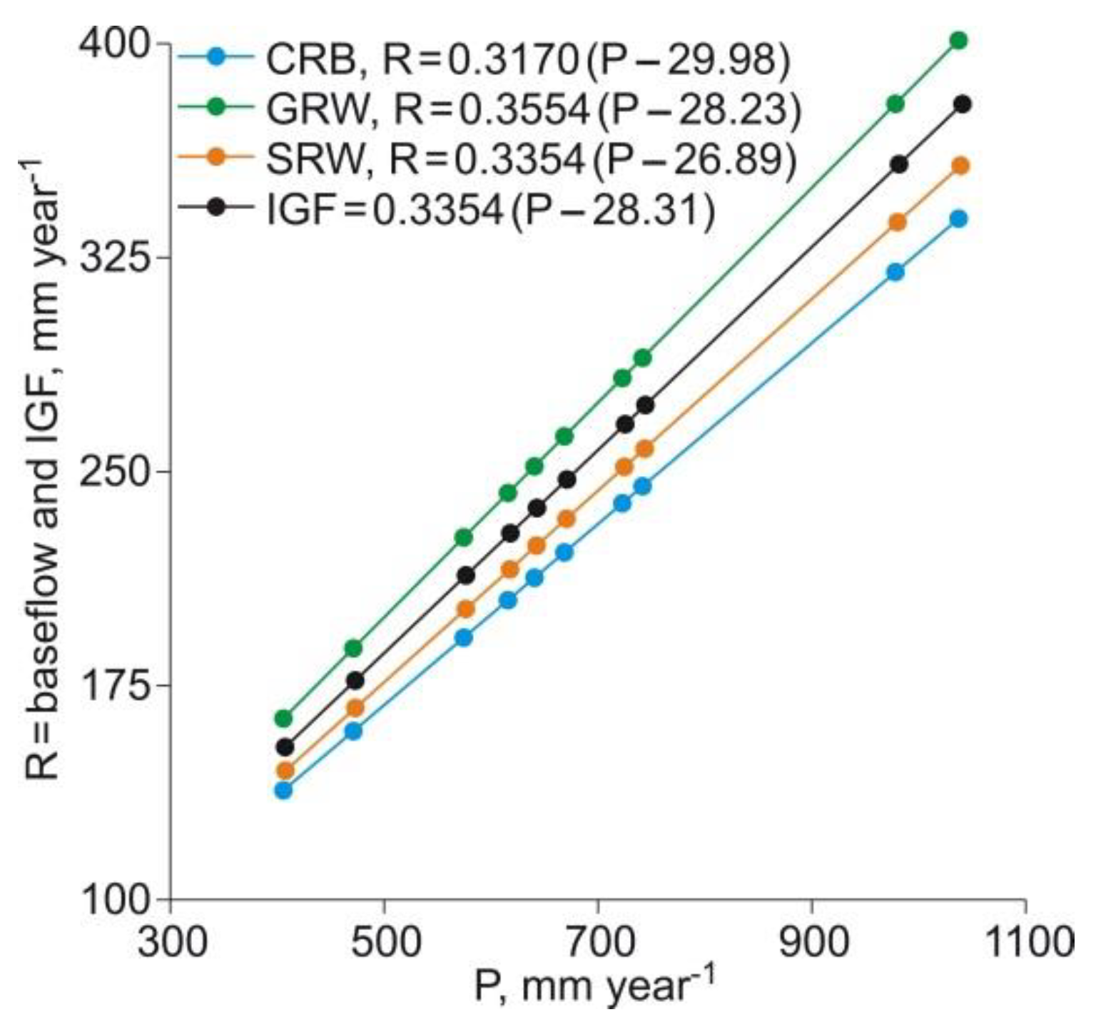
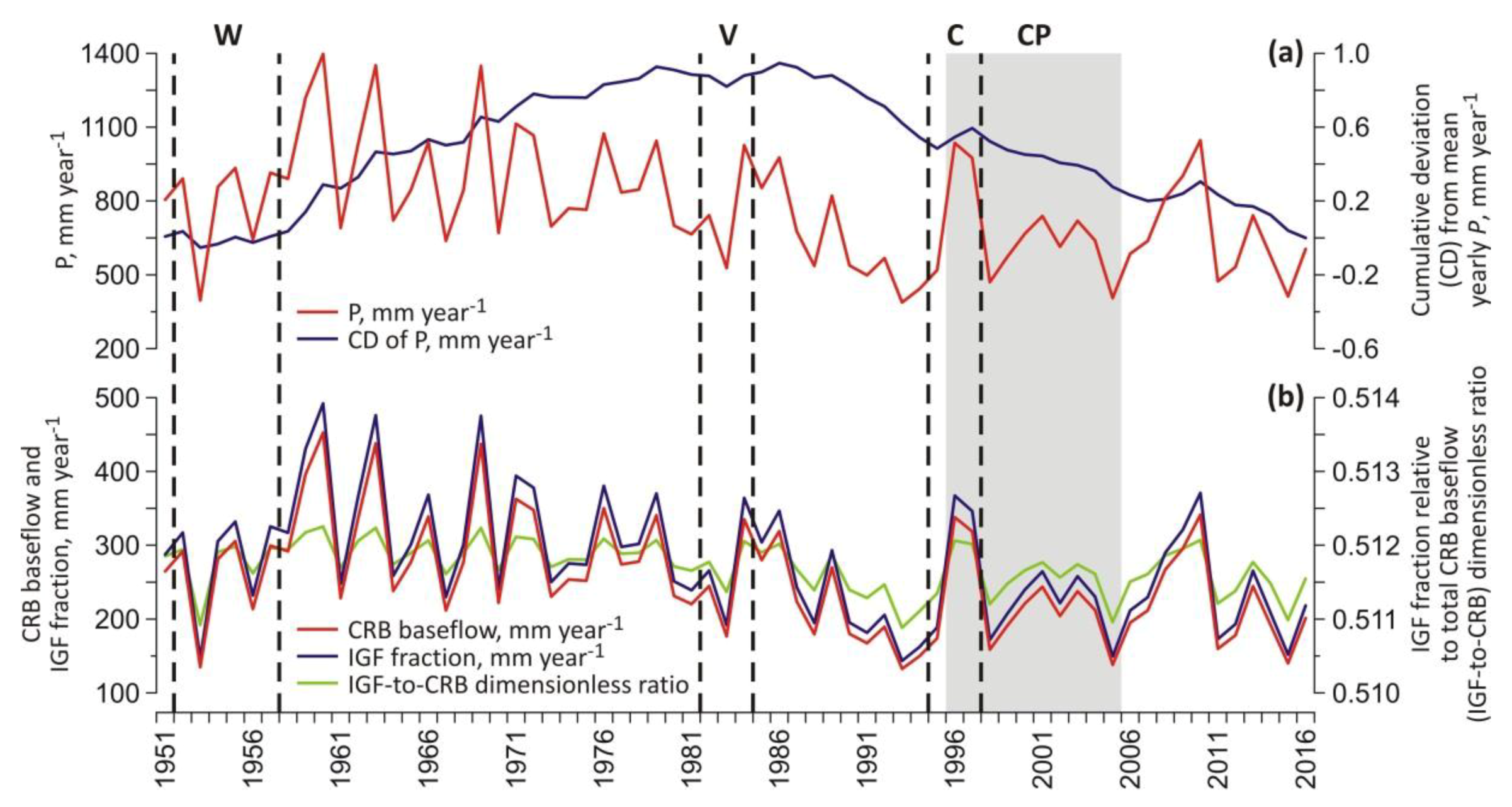
In this area, for the control period (1996–2005), nodal mean R varied within the range 143–332 mm year^–1, which means recharge–precipitation ratios were in the 0.29–0.37 range; the standard deviation of mean R varied within the 39–90 mm year^–1 range, which placed the given coefficients of variation of mean annual R (mean value-to-standard deviation ratio) in the 0.27–0.30 range (

Table 2. For the 10 km × 10 km cells covering the CRB and upstream GRW and SGW contributing areas, the CMB datasets gathered from Alcalá and Custodio (2014, 2015) [34,42].

Cell 1	CRB					GRW					SRW
	S	P 2	CVP	R	CVR	S	P	CVP	R	CVR	S	P	CVP	R	CVR
3200						3.2	894	0.31	315	0.27	0.8	894	0.31	315	0.27
3201	10.4	909	0.33	332	0.27	20.2	909	0.33	332	0.27
3202	60.6	693	0.34	229	0.28	4.8	693	0.34	229	0.28
3203	7.1	486	0.35	143	0.27
3275						1.0	813	0.32	276	0.27	21.7	813	0.32	276	0.27
3276	22.0	668	0.33	206	0.29	14.5	668	0.33	206	0.29	25.0	668	0.33	206	0.29
3277	1.8	517	0.35	153	0.30	1.1	517	0.35	153	0.30
3349						0.1	687	0.32	212	0.27	0.5	687	0.32	212	0.27
3350						2.0	612	0.33	186	0.28	0.5	612	0.33	186	0.28
Sum	101.9					46.9					48.4
SWA 3		692	0.34	227	0.28		787	0.33	269	0.28		736	0.32	239	0.28

¹ Cell ID as in Figure 1c. ² S is surface in km², P and R are, respectively, mean precipitation and mean net aquifer recharge over the control period (1996–2005) in mm year^–1; and CVP and CVR are the dimensionless coefficients of variation of mean P and R over the control period (1996–2005) as fractions. ³ SWA is surface-weighted average.

). For the control period (1996–2005), fitting parameters were calculated to generate the yearly R data series in the CRB and upstream GRW and SRW contributing areas, which are in

Table 3. Fitting parameters for the CRB and upstream GRW and SGW areas.

Parameter 1	CRB	GRW	SRW
Δm	−0.67	−0.66	−0.67
Δσ	−0.73	−0.71	−0.72
mC	227	269	239
σC	63.1	74.9	66.8

¹ Δm and Δσ are dimensionless, and m_C and σ_C are in mm year^–1.

, whereas the generated surface-weighted yearly P and R series are in

Table 4. For the control period (1996–2005), surface-weighted yearly series of (i) P and R in the CRB and in upstream GRW and SRW areas, and (ii) IGF from the GRW and SRW area contributing to CRB.

Year	P 1	Psi 1	R, CRB 1	R, GRW	R, SRW	IGF, GRW+SRW 2
1996	1037.9	1.76	338.5	401.4	357.1	378.9
1997	978.9	1.47	319.8	379.2	337.3	357.9
1998	472.3	−1.08	159.2	188.7	167.4	177.9
1999	575.4	−0.56	191.9	227.5	202.0	214.6
2000	669.5	−0.09	221.7	262.9	233.6	248.0
2001	742.6	0.28	244.9	290.4	258.1	274.0
2002	616.8	−0.35	205.0	243.1	215.9	229.3
2003	723.7	0.19	238.9	283.3	251.8	267.3
2004	641.5	−0.23	212.9	252.4	224.2	238.1
2005	406.9	−1.40	138.5	164.1	145.5	154.7
Mean 3	686.6		227.1	269.3	239.3	240.1
SD	199.2		63.1	74.9	66.8	66.8
CV	0.29		0.28	0.28	0.28	0.28

¹ P and R are, respectively, annual precipitation and net aquifer recharge in mm year⁻¹, and Psi is dimensionless normalized yearly P. ² IGF is interbasin groundwater flow in mm year⁻¹. ³ Mean and SD are mean and standard deviation over the control period (1996–2005) in mm year⁻¹, and CV is dimensionless coefficient of variation as a fraction.

. In each area, yearly R and P series for the control period (1996–2005) were compared. The resulting parametric functions allowed for the extension of the calculated yearly R series to cover the yearly P full record (1951–2016) (Figure 4). Figure 5 shows the full yearly baseflow series generated within the CBR, as well as the yearly surface-weighted IGF series contributed by upstream GRW and SRW areas. As observed, IGF is somewhat higher than baseflow, generated within the CRB. IGF is about 51% of total CRB baseflow.

3.2. Comparison of SWAT Model Results with and without IGF

Based on DEM analysis and after SWAT model implementation, the CRB was discretized into 29 sub-basins. Based on the combination of land uses, soil types, and slope ranges (<2%, 2%–8%, >8%), 149 HRUs were defined. The thresholds for defining HRUs were set to 5% to optimize model processing. The Hargreaves non-global method was used to simulate potential evapotranspiration [68]. As a result, only precipitation and temperature data to run the SWAT model were needed.

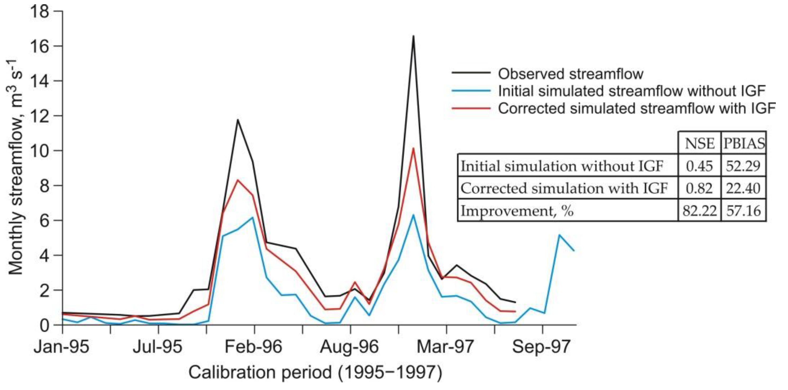
As described in Section 3.1, the IGF from upstream GRW and SRW areas greatly contributes to the Castril River streamflow. For the period 1995−1997, the SWAT model was doubly implemented on a monthly scale with and without IGF. The result was a large difference between observed and initial simulated streamflow when IGF was omitted (Figure 6). When IGF was included as an additional baseflow fraction, the difference between observed and corrected simulated streamflow clearly narrowed. This preliminary trial at model performance showed that the statistics NSE and PBIAS improve when IGF was included (Figure 6). Overall model performance increased about 80% in absolute terms.

3.3. Calibration and Validation of SWAT Model Including IGF

A total of 21 SWAT parameters were optimized using the SUFI-2 algorithm from SWAT-CUP. As described in Section 2.5.2, parameter selection was based on our previous research experiences in similar basins in Southern Spain [64,65]. The SWAT calibration phase covered a 3-year period (1995–1997). The final ranges used and the final fitted values of these parameters are given in

Table 5. Description of parameters used for SWAT model calibration in the CRB.

Parameter 1	Description	Range Used in Calibration	Fitted Value
r_CN2.mgt	Soil Conservation Service (SCS) runoff curve number	−0.1 to 0.1	0.08
v_ALPHA_BF.gw	Baseflow alpha factor (day−1)	0 to 1	0.11
a_GW_DELAY.gw	Groundwater delay time (day)	0 to 60	2.82
a_GWQMN.gw	Threshold depth of water in the shallow aquifer for return flow to occur (mm)	−200 to 1000	898.00
v_GW_REVAP.gw	Groundwater revap coefficient	0.02 to 0.1	0.09
a_RCHRG_DP.gw	Deep aquifer percolation fraction	−0.05 to 0.05	0.04
a_REVAPMN.gw	Threshold depth of water in shallow aquifer for revap or percolation to deep aquifer to occur (mm)	−500 to 500	−61.00
v_CANMX.hru	Maximum canopy storage (mm)	0 to 8	0.47
v_EPCO.bsn	Plant uptake compensation factor	0.5 to 1	0.56
v_ESCO.bsn	Soil evaporation compensation factor	0.3 to 0.8	0.61
r_SOL_AWC.sol	Available water capacity of the soil layer (mm H2O/mm soil)	−0.02 to 0.02	−0.02
v_LAT_TTIME.hru	Lateral flow travel time (day)	0 to 180	76.50
v_SLSOIL.hru	Slope length for lateral subsurface flow (m)	0 to 150	1.35
r_SLSUBBSN.hru	Average slope length (m)	−0.5 to 0.5	0.08
r_HRU_SLP.hru	Average slope steepness (m/m)	−0.5 to 0.5	0.40
v_OV_N.hru	Manning’s ‘n’ value for overland flow	0.01 to 1	0.61
r_CH_S1.sub	Average slope of tributary channels (m/m).	−0.5 to 0.5	0.26
v_CH_N1.sub	Manning’s ‘n’ value for the tributary channels	0.01 to 30	1.68
r_CH_S2.rte	Average slope of main channel along the channel length (m/m)	−0.5 to 0.5	−0.04
v_CH_N2.rte	Manning’s ‘n’ value for the main channel	0.01 to 0.3	0.04
v_SURLAG.bsn	Surface runoff lag coefficient	0.05 to 24	20.71

¹ (r_) refers to relative change, i.e., the current parameter must be multiplied by (1 + the value obtained in calibration), (v_) means that the existing parameter value must be replaced by the value obtained in calibration, and (a_) refers to absolute change, i.e., the fitted value must be added to the existing value of the parameter.

.

The magnitude of calibrated GW_REVAP, ESCO, LAT_TTIME, GWQMN, and ALPHA_BF parameters is quite similar to those obtained with similar orography, geology, climate, and land use [64,65]. The ESCO is also similar to that fitted in other Mediterranean karst areas, where yearly actual evapotranspiration is typically 0.7–0.9 fold yearly precipitation [26,27,46]. The low value of ALPHA_BF indicates a slow aquifer response [69]. This is corroborated by the long-delayed responses to recharge events in similar karst aquifers in the region, reported by Moral et al. (2008) [70].

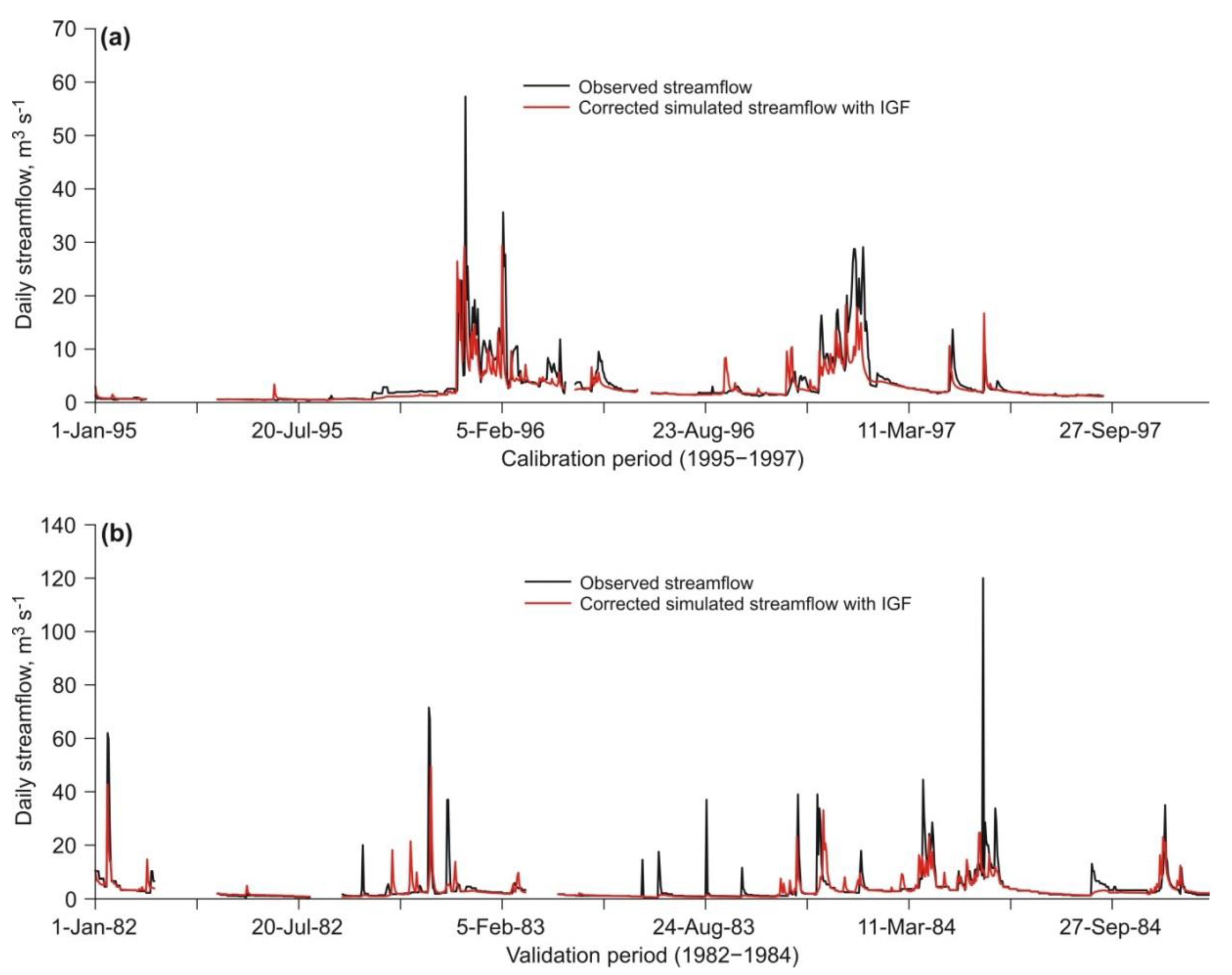
Corrected streamflow records with IGF were used for model calibration (1995–1997) and validation (1982–1984) phases. Observed streamflow was compared to corrected simulated streamflow on monthly (Figure 7) and daily (Figure 8) scales during the calibration and validation periods. In the CRB, the fitted SWAT model replicated, almost identically, the trend of the streamflow hydrograph. The higher fluctuations in the simulated peaks and the lower ones in low flows were found, both in monthly and daily streamflow simulations.

As observed in Figure 8, low flows predominate in the CRB daily streamflow record. As many other SWAT models reported for other similar aquifer-fed karst areas, the SWAT model performance for high and normal flows decreased in the face of predominant low flows [65,71]. Therefore, following the suggestion of Krause et al. (2005) [72], NSE and InNSE were used to measure, respectively, the high and the low flows, to reduce the problem of the squared differences and the resulting sensitivity to extreme values of NSE. Calibration and validation of monthly corrected streamflow showed good agreement of simulated and observed data, as indicated by the model performance statistics for monthly and daily simulations given in

Table 6. SWAT model performance statistics for corrected simulated monthly and daily streamflow during calibration and validation phases.

Statistic	Time Step	Calibration	Validation
NSE	Monthly	0.77	0.8
R2	Monthly	0.92	0.89
PBIAS	Monthly	19.82	17.25
RSR	Monthly	0.48	0.44
lnNSE	Daily	0.81	0.64

.

As finally deduced, the SWAT model performs well and can be used for further analysis in the CRB and in other similar high-permeability bedrock basins, the baseflow of which is strongly determined by IGF. For this, there must be a confident evaluation of IGF or, at minimum, a reliable external evaluation available. In this paper, the CMB method and the available CMB datasets in continental Spain [34,42] were used for this purpose. However, as described for other groundwater and surface water coupling models, the SWAT-CMB application presented here reveals the following overall problems: (1) the spatial (size and volume) and temporal (renovation rate) scales of groundwater and surface water bodies differ, whereas the coupling model can only simulate the same spatial and temporal scale in both types of bodies; (2) the coupling models had defects in the coupling mechanism processing, which demanded substantial simplification of the coupling process, thereby causing model distortion; and (3) this coupling model was established for a certain region or a specific problem and, although good results have been achieved, there is no general adaptability, so additional hydrogeological knowledge of local applications is needed to consider the changes in scale effects and actual flow conditions.

4. Conclusions

This paper presents the combined application of the SWAT model and the CMB method to model streamflow in the CRB, a representative high-permeability bedrock basin where the streamflow is significantly determined by IGF from upstream contributing areas. The CMB method and available CMB datasets in continental Spain were used for the IGF that adds to the baseflow generated within the CRB. The SWAT model performance improved noticeably when simulated streamflow with IGF was used. Using the CMB datasets for streamflow correction, the SWAT model showed good performance both in daily and monthly simulations. Some overall remarks from this research are highlighted below.

The influence of IGF on basins like the CRB is remarkable. Therefore, IGF must be considered to improve water resource evaluation and management in this kind of basin located in the headwater of large river watersheds. In the CRB, IGF means about 51% of total baseflow. We do not suggest using the SWAT model alone for modeling of these aquifer-fed mountain basins. It must be coupled with other specific methods to accurately assess IGF. The CMB was revealed to be a suitable method for IGF, because of the favorable hydrogeological setting and the negligible groundwater abstraction, which allowed for equivalent net aquifer recharge to the baseflow contributing to streamflow in the headwater of large river watersheds. In other areas that reflect different patterns of groundwater use and hydrogeological features, assessment of IGF must rely on other techniques coupled with the SWAT model.

References

- Trolle, D.; Hamilton, D.P.; Hipsey, M.R.; Bolding, K.; Bruggeman, J.; Mooij, W.M.; Janse, J.H.; Nielsen, A.; Jeppesen, E.; Elliott, A.; et al. A community–based framework for aquatic ecosystem models. Hydrobiologia 2012, 683, 25–34. [Google Scholar] [CrossRef]
- Hojberg, A.L.; Refsgaard, J.C. Model uncertainty-parameter uncertainty versus conceptual models. Water Sci. Technol. 2005, 52, 177–186. [Google Scholar] [CrossRef] [PubMed]
- Beven, K. Towards integrated environmental models of everywhere: Uncertainty, data and modelling as a learning process. Hydrol. Earth Syst. Sci. 2007, 11, 460–467. [Google Scholar] [CrossRef]
- Alcalá, F.J.; Martínez-Valderrama, J.; Robles-Marín, P.; Guerrera, F.; Martín-Martín, M.; Raffaelli, G.; Tejera de León, J.; Asebriy, L. A hydrological-economic model for sustainable groundwater use in sparse-data drylands: Application to the Amtoudi Oasis in southern Morocco, northern Sahara. Sci. Total Environ. 2015, 537, 309–322. [Google Scholar] [CrossRef]
- Francesconi, W.; Srinivasan, R.; Pérez-Miñana, E.; Willcock, S.P.; Quintero, M. Using the Soil and Water Assessment Tool (SWAT) to model ecosystem services: A systematic review. J. Hydrol. 2016, 535, 625–636. [Google Scholar] [CrossRef]
- Arnold, J.G.; Srinivasan, R.; Muttiah, R.S.; Williams, J.R. Large area hydrologic modeling and assessment Part I: Model development. J. Am. Water Resour. Assoc. 1998, 34, 73–89. [Google Scholar] [CrossRef]
- Molina-Navarro, E.; Andersen, H.E.; Nielsen, A.; Thodsen, H.; Trolle, D. Quantifying the combined effects of land use and climate changes on stream flow and nutrient loads: A modelling approach in the Odense Fjord catchment (Denmark). Sci. Total Environ. 2018, 621, 253–264. [Google Scholar] [CrossRef]
- Blanco-Gómez, P.; Jimeno-Sáez, P.; Senent-Aparicio, J.; Pérez-Sánchez, J. Impact of Climate Change on Water Balance Components and Droughts in the Guajoyo River Basin (El Salvador). Water 2019, 11, 2360. [Google Scholar] [CrossRef] [Green Version]
- Senent-Aparicio, J.; Liu, S.; Pérez-Sánchez, J.; López-Ballesteros, A.; Jimeno-Sáez, P. Assessing Impacts of Climate Variability and Reforestation Activities on Water Resources in the Headwaters of the Segura River Basin (SE Spain). Sustainability 2018, 10, 3277. [Google Scholar] [CrossRef] [Green Version]
- Fu, B.; Merritt, W.S.; Croke, B.F.W.; Weber, T.R.; Jakeman, A.J. A review of catchment-scale water quality and erosion models and a synthesis of future prospects. Environ. Model. Softw. 2019, 114, 75–97. [Google Scholar] [CrossRef]
- Luo, Y.; Arnold, J.; Allen, P.; Chen, X. Baseflow simulation using SWAT model in an inland river basin in Tianshan Mountains, Northwest China. Hydrol. Earth Syst. Sci. 2012, 16, 1259–1267. [Google Scholar] [CrossRef] [Green Version]
- Ficklin, D.L.; Luo, Y.; Zhang, M. Watershed Modelling of Hydrology and Water Quality in the Sacramento River Watershed, California. Hydrol. Process. 2012, 27, 236–250. [Google Scholar] [CrossRef]
- Genereux, D.P.; Jordan, M.T.; Carbonell, D. A pired-watershed budget study to quantify interbasin groundwater flow in a lowland rain forest. Costa Rica. Water Resour. Res. 2005, 41, W04011. [Google Scholar] [CrossRef]
- Nguyen, V.T.; Dietrich, J.; Uniyal, B. Modeling interbasin groundwater flow in karst areas: Model development, application, and calibration strategy. Environ. Modell. Softw. 2020, 124, 104606. [Google Scholar] [CrossRef]
- Zanon, C.; Genereux, D.P.; Oberbauer, S.F. Use of a watershed hydrologic model to estimate interbasin groundwater flow in a Costa Rican rainforest. Hydrol. Process. 2014, 28, 3670–3680. [Google Scholar] [CrossRef]
- Rahayuningtyas, C.; Wu, R.S.; Anwar, R.; Chiang, L.C. Improving avswat stream flow simulation by incorporating groundwater recharge prediction in the upstream Lesti watershed, East Java, Indonesia. Terr. Atmos. Ocean. Sci. 2014, 25, 881–892. [Google Scholar] [CrossRef] [Green Version]
- Han, M.; Zhao, C.Y.; Šimůnek, J.; Feng, G. Evaluating the impact of groundwater on cotton growth and root zone water balance using Hydrus-1D coupled with a crop growth model. Agric. Water Manag. 2015, 160, 64–75. [Google Scholar] [CrossRef] [Green Version]
- Obuobie, E. Estimation of Groundwater Recharge in the Context of Future Climate Change in the White Volta River Basin, West Africa. Germany. Ph.D. Thesis, Rheinischen Friedrich-Wilhelms-Universität, Bonn, Germany, 2008; 165p. [Google Scholar]
- Alcalá, F.J.; Martín-Martín, M.; Guerrera, F.; Martínez-Valderrama, J.; Marín, P.R. A feasible methodology for groundwater resource modelling for sustainable use in sparse-data drylands: Application to the Amtoudi Oasis in the northern Sahara. Sci. Total Environ. 2018, 630, 1246–1257. [Google Scholar] [CrossRef]
- Kim, N.W.; Chung, I.M.; Won, Y.S.; Arnold, J.G. Development and application of the integrated SWAT-MODFLOW model. J. Hydrol. 2008, 356, 1–16. [Google Scholar] [CrossRef]
- Bouaziz, L.; Weerts, A.; Schellekens, J.; Sprokkereef, E.; Stam, J.; Savenije, H.; Hrachowitz, M. Redressing the balance: Quantifying net intercatchment groundwater flows. Hydrol. Earth Syst. Sci. 2018, 22, 6415–6434. [Google Scholar] [CrossRef] [Green Version]
- Palanisamy, B.; Workman, S.R. Hydrologic modeling of flow through sinkholes located in streambeds of Cane Run stream, Kentucky. J. Hydrol. Eng. 2014, 20, 04014066. [Google Scholar] [CrossRef]
- Malagó, A.; Efstathiou, D.; Bouraoui, F.; Nikolaidis, N.P.; Franchini, M.; Bidoglio, G.; Kritsotakis, M. Regional scale hydrologic modeling of a karst-dominant geomorphology: The case study of the island of Crete. J. Hydrol. 2016, 540, 64–81. [Google Scholar] [CrossRef]
- Baffaut, C.; Benson, V.W. Modeling flow and pollutant transport in a karst watershed with SWAT. Trans. ASABE 2009, 52, 469–479. [Google Scholar] [CrossRef]
- Nikolaidis, N.P.; Bouraoui, F.; Bidoglio, G. Hydrologic and geochemical modeling of a karstic Mediterranean watershed. J. Hydrol. 2013, 477, 129–138. [Google Scholar] [CrossRef]
- Alcalá, F.J.; Cantón, Y.; Contreras, S.; Were, A.; Serrano-Ortiz, P.; Puigdefábregas, J.; Solé-Benet, A.; Custodio, E.; Domingo, F. Diffuse and concentrated recharge evaluation using physical and tracer techniques: Results from a semiarid carbonate massif aquifer in southeastern Spain. Environ. Earth Sci. 2011, 63, 541–557. [Google Scholar] [CrossRef] [Green Version]
- Andreu, J.M.; Alcalá, F.J.; Vallejos, Á.; Pulido-Bosch, A. Recharge to aquifers in SE Spain: Different approaches and new challenges. J. Arid Environ. 2011, 75, 1262–1270. [Google Scholar] [CrossRef]
- Rutledge, A.T.; Mesko, T.O. Estimated Hydrologic Characteristics of Shallow Aquifer Systems in the Valley and Ridge, the Blue Ridge, and the Piedmont Physiographic Provinces Based on Analysis of Streamflow Recession and Base Flow; U.S. Geological Survey: Reston, VA, USA, 1996; 58p.
- Lim, K.J.; Engel, B.A.; Tang, Z.; Choi, J.; Kim, K.S.; Muthukrishnan, S.; Tripathy, D. Automated web GIS based hydrograph analysis tool, WHAT. J. Am. Water Resour. Assoc. 2005, 1407–1416. [Google Scholar] [CrossRef]
- Plesca, I.; Timbe, E.; Exbrayat, J.-F.; Windhorst, D.; Kraft, P.; Crespo, P.; Vaché, K.B.; Frede, H.-G.; Breuer, L. Model intercomparison to explore catchment functioning: Results from a remote montane tropical rainforest. Ecol. Model. 2012, 239, 3–13. [Google Scholar] [CrossRef] [Green Version]
- Lee, J.; Kim, J.; Jang, W.S.; Lim, K.J.; Engel, B.A. Assessment of Baseflow Estimates Considering Recession Characteristics in SWAT. Water 2018, 10, 371. [Google Scholar] [CrossRef] [Green Version]
- Lerner, D.N.; Issar, A.S.; Simmers, I. Groundwater recharge. A guide to understanding and estimating natural recharge. In IAH International Contributions to Hydrogeology; Heise: Hannover, Germany, 1990; 345p. [Google Scholar]
- Batelaan, O.; De Smedt, F. GIS-based recharge estimation by coupling surface-subsurface water balances. J. Hydrol. 2007, 337, 337–355. [Google Scholar] [CrossRef]
- Alcalá, F.J.; Custodio, E. Spatial average aquifer recharge through atmospheric chloride mass balance and its uncertainty in continental Spain. Hydrol. Process. 2014, 28, 218–236. [Google Scholar] [CrossRef]
- Scanlon, B.R.; Healy, R.W.; Cook, P.G. Choosing appropriate techniques for quantifying groundwater recharge. Hydrogeol. J. 2002, 10, 18–39. [Google Scholar] [CrossRef]
- McMahon, P.B.; Plummer, L.N.; Bohlke, J.K.; Shapiro, S.D.; Hinkle, S.R. A comparison of recharge rates in aquifers of the United States based on groundwater-based data. Hydrogeol. J. 2011, 19, 779–800. [Google Scholar] [CrossRef]
- Claasen, H.C.; Reddy, M.M.; Halm, D.R. Use of the chloride ion in determining hydrologic-basin water budgets: A 3-year case study in the San Juan Mountains, Colorado, USA. J. Hydrol. 1986, 85, 49–71. [Google Scholar] [CrossRef]
- Dettinger, M.D. Reconnaissance estimates of natural recharge to desert basins in Nevada, USA, by using chloride-balance calculations. J. Hydrol. 1989, 106, 55–78. [Google Scholar] [CrossRef]
- Wood, W.W.; Sanford, W.E. Chemical and isotopic methods for quantifying ground-water recharge in a regional, semiarid environment. Ground Water 1995, 33, 458–468. [Google Scholar] [CrossRef]
- Sami, K.; Hughes, D.A. A comparison of recharge estimates to a fractured sedimentary aquifer in South Africa from a chloride mass balance and an integrated surface-subsurface model. J. Hydrol. 1996, 179, 111–136. [Google Scholar] [CrossRef]
- Scanlon, B.R.; Keese, K.E.; Flint, A.L.; Flint, L.E.; Gaye, C.B.; Edmunds, W.M.; Simmers, I. Global synthesis of groundwater recharge in semiarid and arid regions. Hydrol. Process. 2006, 20, 3335–3370. [Google Scholar] [CrossRef]
- Alcalá, F.J.; Custodio, E. Natural uncertainty of spatial average aquifer recharge through atmospheric chloride mass balance in continental Spain. J. Hydrol. 2015, 524, 642–661. [Google Scholar] [CrossRef]
- Paz, C.; Alcalá, F.J.; Carvalho, J.M.; Ribeiro, L. Current uses of ground penetrating radar in groundwater-dependent ecosystems research. Sci. Total Environ. 2017, 595, 868–885. [Google Scholar] [CrossRef]
- Capel-Molina, J.J. Los Climas de España; Oikos-Tau: Barcelona, Spain, 1981; 403p. [Google Scholar]
- Trigo, R.; Pozo-Vázquez, D.; Osborn, T.; Castro-Díez, Y.; Gámiz-Fortis, S.; Esteban-Parra, M. North Atlantic oscillation influence on precipitation, river flow and water resources in the Iberian peninsula. Int. J. Climatol. 2004, 24, 925–944. [Google Scholar] [CrossRef]
- Vanderlinden, K.; Giraldez, J.V.; Van Meirvenne, M. Assessing Reference Evapotranspiration by the Hargreaves Method in Southern Spain. J. Irrig. Drain. Eng. 2004, 130, 184–191. [Google Scholar] [CrossRef]
- Azéma, J.; Foucault, A.; Fourcade, E.; García–Hernández, M.; González–Donoso, J.M.; Linares, D.; López–García, A.C.; Rivas, P.; Vera, J.A. Las Microfacies del Jurásico y Cretácico de las Zonas Externas de las Cordilleras Béticas; Servicio de Publicaciones de la Universidad de Granada: Granada, Spain, 1979. [Google Scholar]
- Vera, J.A. Geología de España, 1st ed.; Sociedad Geológica de España e Instituto Geológico y Minero de España, Ministerio de Educación y Ciencia: Madrid, Spain, 2004; 884p. [Google Scholar]
- Sanz de Galdeano, C.; Peláez, J.A. La Cuenca de Guadix–Baza. Estructura, Tectónica Activa, Sismicidad, Geomorfología y Dataciones Existentes; Universidad de Granada–CSIC: Granada, Spain, 2007; 351p. [Google Scholar]
- IGME. Hydrogeological Map of Spain, Scale 1:200,000; Sheet nº 78, Baza; Geological Survey of Spain, Memory and Maps. 1988. Available online: http://info.igme.es/cartografiadigital/tematica/Hidrogeologico200.aspx (accessed on 20 January 2020).
- IGME. Hydrogeological Map of Spain, Scale 1:200,000. Sheet nº 71, Villacarrillo; Geological Survey of Spain, Memory and Maps. 1995. Available online: http://info.igme.es/cartografiadigital/tematica/Hidrogeologico200.aspx (accessed on 20 January 2020).
- IGME. Proyecto para la actualización de la infraestructura hidrogeológica de las Unidades 05.01 Sierra de Cazorla, 05.02 Quesada-Castril, 07.07 Sierras de Segura-Cazorla y el Carbonatado de la Loma de Úbeda; Geological Survey of Spain and General Directorate for Water Planning; Ministry of Industry: Madrid, Spain, 2001. (In Spanish) [Google Scholar]
- Peralta-Maraver, I.; López-Rodríguez, M.J.; de Figueroa, J.T. Structure, dynamics and stability of a Mediterranean river food web. Mar. Freshwater Res. 2017, 68, 484–495. [Google Scholar] [CrossRef]
- Alcalá, F.J.; Custodio, E. Atmospheric chloride deposition in continental Spain. Hydrol. Process. 2008, 22, 3636–3650. [Google Scholar] [CrossRef]
- Alcala, F.J.; Custodio, E. Using the Cl/Br ratio as a tracer to identify the origin of salinity in aquifers in Spain and Portugal. J. Hydrol. 2008, 359, 189–207. [Google Scholar] [CrossRef]
- Hurrell, J.W. Decadal trends in the North Atlantic Oscillation, regional temperatures and precipitation. Nature 1995, 269, 676–679. [Google Scholar] [CrossRef] [Green Version]
- Raposo, J.R.; Dafonte, J.; Molinero, J. Assessing the impact of future climate change on groundwater recharge in Galicia-Costa, Spain. Hydrogeol. J. 2013, 21, 459–479. [Google Scholar] [CrossRef]
- Barberá, J.A.; Jódar, J.; Custodio, E.; González-Ramón, A.; Jiménez-Gavilán, P.; Vadillo, I.; Pedrera, A.; Martos-Rosillo, S. Groundwater dynamics in a hydrologically-modified alpine watershed from an ancient managed recharge system (Sierra Nevada National Park, Southern Spain): Insights from hydrogeochemical and isotopic information. Sci. Total Environ. 2018, 640–641, 874–893. [Google Scholar] [CrossRef]
- Pulido-Velazquez, D.; Collados-Lara, A.J.; Alcalá, F.J. Assessing impacts of future potential climate change scenarios on aquifer recharge in continental Spain. J. Hydrol. 2018, 567, 803–819. [Google Scholar] [CrossRef]
- Nathan, R.J.; McMahon, T.A. Evaluation of automated techniques for base-flow and recession analyses. Water Resour. Res. 1990, 26, 1465–1473. [Google Scholar] [CrossRef]
- Arnold, J.G.; Allen, P.M.; Muttiah, R.; Bernhardt, G. Automated Base Flow Separation and Recession Analysis Techniques. Ground Water 1995, 33, 1010–1018. [Google Scholar] [CrossRef]
- Meaurio, M.; Zabaleta, A.; Angel, J.; Srinivasan, R.; Antigüedad, I. Evaluation of SWAT models performance to simulate streamflow spatial origin. The case of a small forested watershed. J. Hydrol. 2015, 525, 326–334. [Google Scholar] [CrossRef]
- Arnold, J.G.; Allen, P.M. Automated Methods for Estimating Baseflow and Ground Water Recharge from Streamflow Records. JAWRA J. Am. Water Resour. Assoc. 1999, 35, 411–424. [Google Scholar] [CrossRef]
- Senent-Aparicio, J.; Pérez-Sánchez, J.; Carrillo-García, J.; Soto, J. Using SWAT and Fuzzy TOPSIS to Assess the Impact of Climate Change in the Headwaters of the Segura River Basin (SE Spain). Water 2017, 9, 149. [Google Scholar] [CrossRef] [Green Version]
- Jimeno-Sáez, P.; Senent-Aparicio, J.; Pérez-Sánchez, J.; Pulido-Velazquez, D. A Comparison of SWAT and ANN models for daily runoff simulation in different climatic zones of peninsular Spain. Water 2018, 10, 192. [Google Scholar] [CrossRef] [Green Version]
- Abbaspour, K.C.; Rouholahnejad, E.; Vaghefi, S.; Srinivasan, R.; Yang, H.; Kløve, B. A continental-scale hydrology and water quality model for Europe: Calibration and uncertainty of a high-resolution large-scale SWAT model. J. Hydrol. 2015, 524, 733–752. [Google Scholar] [CrossRef] [Green Version]
- Moriasi, D.N.; Wilson, B.N.; Douglas-Mankin, K.R.; Arnold, J.G.; Gowda, P.H. Hydrologic and water quality models: Use, calibration, and validation. Trans. ASABE 2012, 55, 1241–1247. [Google Scholar] [CrossRef]
- Hargreaves, G.H.; Samani, Z.A. Estimating potential evapotranspiration. J. Irrig. Drain. Div. ASCE 1982, 108, 225–230. [Google Scholar]
- Arnold, J.G.; Kiniry, J.R.; Srinivasan, R.; Williams, J.R.; Haney, E.B.; Neitsch, S.L. Soil and Water Assessment Tool—Input/Output Documentation—Version 2012. Available online: http://swat.tamu.edu/documentation/ (accessed on 20 December 2019).
- Moral, F.; Cruz-Sanjulian, J.J.; Olias, M. Geochemical evolution of groundwater in the carbonate aquifers of Sierra de Segura (Betic Cordillera, Southern Spain). J. Hydrol. 2008, 360, 281–296. [Google Scholar] [CrossRef]
- Senent-Aparicio, J.; Jimeno-Sáez, P.; Bueno-Crespo, A.; Pérez-Sánchez, J.; Pulido-Velazquez, D. Coupling machine-learning techniques with SWAT model for instantaneous peak flow prediction. Biosyst. Eng. 2019, 177, 67–77. [Google Scholar] [CrossRef]
- Krause, P.; Boyle, D.P.; Base, F. Comparison of different efficiency criteria for hydrological model assessment. Adv. Geosci. 2005, 5, 89–97. [Google Scholar] [CrossRef] [Green Version]
Figure 1.
(a) Location of the Castril River basin (CRB) within the Guadalquivir River watershed (GRW) in southern Spain, adjacent to the Segura River watershed (SRW). (b) Discretization of the CRB and 29 sub-basins using the 25 m resolution Digital Elevation Model (DEM) from the Spanish National Geographic Institute, showing other features cited in the text. (c) After the Geological Survey of Spain (IGME) (1988, 1995, 2001) [50,51,52] and direct field observations, a hydrogeological map of the CRB (scale 1:200,000), the schematic hydrogeological functioning of the CRB and the hydraulically connected upstream GRW and SRW contributing areas, a hydrogeological cross-section A–A′ showing aquifer dimensions, CBR location, groundwater divides and flow paths, and the 10 km x 10 km cells for distributed net aquifer recharge (R) in the part of continental Spain [34,42] covered in the study area was developed.
Figure 2.
Land-use map (scale 1:25,000) from the Andalusian Environmental Information Network (REDIAM).
Figure 3.
Flow diagram for the coupled Soil and Water Assessment Tool (SWAT) model and chloride mass balance (CMB) method application to model streamflow of hydrological basins subjected to interbasin groundwater flow (IGF).
Figure 4.
For the control period (1996–2005), parameterization of yearly P–R functions in the CRB and upstream GRW and SRW contributing areas; yearly R equals yearly baseflow. Yearly IGF series refers to the surface-weighed sum of upstream R = baseflow from GRW and SRW areas contributing to the CRB streamflow. In all cases, the Pearson coefficient of correlation is 1.
Figure 5.
For the full period (1951–2016), (a) surface-weighted yearly P series in the area compiled from the Spanish National Weather Service (AEMET) grid version 1.0 and cumulative deviation (CD) from mean yearly P in mm year−1; and (b) generated yearly baseflow series in the CRB and yearly surface-weighed IGF series from upstream GRW and SRW contributing areas in mm year−1, and IGF fraction relative to total CRB baseflow (IGF–CRB) dimensionless ratio. The control period (1996–2005) is grey shallowed (CP). Vertical dotted lines indicate selected time intervals for the SWAT model warm-up (W), calibration (C), and validation (V) phases.
Figure 6.
For the selected calibration period (1995−1997) and on a monthly scale, observed streamflow compared to (i) initial simulated streamflow without IGF and (ii) corrected simulated streamflow with IGF. The statistics NSE and PBIAS show the model performance achieved in each simulation.
Figure 7.
On a monthly scale, observed streamflow compared to corrected simulated streamflow with SWAT model for the (a) calibration and (b) validation phases.
Figure 8.
On a daily scale, observed streamflow compared to corrected simulated streamflow with SWAT model for the (a) calibration and (b) validation phases.