A Cost-Effectiveness Protocol for Flood-Mitigation Plans Based on Leeds’ Boxing Day 2015 Floods


1
School of Mathematics and Leeds Institute for Fluid Dynamics, University of Leeds, Leeds LS2 9JT, UK
2
INRAE, UR ETNA, Université Grenoble Alpes, 38000 Grenoble, France
*
Author to whom correspondence should be addressed.
Water 2020, 12(3), 652; https://doi.org/10.3390/w12030652
Submission received: 10 January 2020
/
Revised: 9 February 2020
/
Accepted: 21 February 2020
/
Published: 28 February 2020
(This article belongs to the Special Issue Challenges and Perspectives in Flood Risk Management and Resilience)
Abstract
:Inspired by the Boxing Day 2015 flood of the River Aire in Leeds, UK, and subsequent attempts to mitigate adverse consequences of flooding, the goals considered are: (i) to revisit the concept of flood-excess volume (FEV) as a complementary diagnostic for classifying flood events; (ii) to establish a new roadmap/protocol for assessing flood-mitigation schemes using FEV; and, (iii) to provide a clear, graphical cost-effectiveness analysis of flood mitigation, exemplified for a hypothetical scheme partially based on actual plans. We revisit the FEV concept and present it as a three-panel graph using thresholds and errors. By re-expressing FEV as a -deep square lake of equivalent capacity, one can visualise its dimensions in comparison with the river valley considered. Cost-effectiveness of flood-mitigation measures is expressed within the FEV square-lake; different scenarios of our hypothetical flood-mitigation scheme are then presented and assessed graphically, with each scenario involving a combination, near and further upstream of Leeds, of higher (than existing) flood-defence walls, enhanced flood-plain storage sites, giving-room-to-the-river bed-widening and natural flood management. Our cost-effectiveness analysis is intended as a protocol to compare and choose between flood-mitigation scenarios in a quantifiable and visual manner, thereby offering better prospects of being understood by a wide audience, including citizens and city-council planners. Using techniques of data analysis combined with general river hydraulics, common-sense and upper-bound estimation, we offer an accessible check of flood-mitigation plans.
1. Introduction
Precipitation records show that, whilst annual rainfall has remained roughly constant in the United Kingdom (UK) in recent decades, within that period there has been an increase and decrease in, respectively, winter and summer rainfall [1]. The spatial and temporal variability of precipitation is also changing. Moreover, though the amount of summer rainfall has decreased overall, it has contemporaneously intensified. The frequency and intensity of extreme-rainfall events has increased, with similar trends observed globally in the extratropical latitudes [1,2]. Heavy precipitation can have disastrous impacts via floods; estimated costs of the 2015/16 winter flooding in the UK alone are between M and M [3]. Damage estimates given for this flood were exceeded by far in earlier floods in the UK (e.g., 2000, 2007, cf. [4]). Flooding is characterized as either fluvial, concerning river flooding, for example due to large-scale winter rainfall, or pluvial, concerning surface water or flash floods, for example due to localized downpours in summer. This increase in damage due to both fluvial and pluvial flooding highlights the need for effective flood-mitigation measures. Such measures are generally engineering-based (e.g., storage reservoirs, defence walls) or nature-based (e.g., catchment-wide tree planting); a suite of these different measures typically constitutes a catchment- or city-wide flood-mitigation scheme [5].
Stakeholder involvement at several implementation phases of flood-mitigation plans is becoming increasingly common, but the technical complexity of some strategies, often involving multiple and disparate measures, hampers enlightened decision-making [6,7]. There is therefore a need for educational tools that facilitate understanding and communication of the efficacy of complex flood-mitigation strategies, additionally because “...these [normative] debates are not held in an open and inclusive way, incorporating the views of all stakeholders” [5]. Here we revisit the concept of flood-excess volume (FEV) to analyse a flood event in a direct manner, with a view to assessing flood-mitigation plans and decision-making via a novel graphical cost-effectiveness analysis. In particular, FEV quantifies the size of a flood event and can be used to concisely partition the effectiveness of individual measures in a flood-mitigation scheme. We focus here on the so-called “Boxing Day Flood” in 2015 of the River Aire in Yorkshire, UK, due to its national publicity at the time, our familiarity with this river, and the availability of both analysable data and interrogable concrete (local) government flood-mitigation plans. While the River Aire case study is specific, it serves to demonstrate, to both decision-makers and citizens, that it is possible to provide a first-order check on flood-mitigation plans using only basic and/or limited means. Such means may be limited because the mitigation plans disseminated are rather concise and/or because detailed data are difficult to obtain, in which case educated guesses and estimates are nonetheless needed to provide a reasonably comprehensive picture to explore and discuss possible scenarios. The cost-effectiveness analysis developed here enables users: (i) to examine rapidly several scenarios to select promising candidates at a preliminary stage; (ii) to check the outcomes of complicated computer simulations, thereby providing an executive summary thereof; and, (iii) to explore complementary scenarios emerging from stakeholders’ ideas at a later stage.
A brief description of the River Aire flood event follows. The Boxing Day floods occurred on 26 and 27 December 2015 in Yorkshire, UK, primarily affecting the River Aire and River Calder; these floods merited high-profile coverage in diverse national media (e.g., Reference [8]). The Aire originates in the Yorkshire Dales and flows roughly eastwards to merge with the Ouse and Humber rivers before finally flowing into the North Sea via the Humber estuary. There was severe flooding, particularly in and around Leeds, see Figure 1 and Figure 2 for flood-plain maps and photographs, with numerous river-level gauges exceeding previous record highs. For example, flood levels recorded on gauges at Armley (circa 2 km upstream of Leeds city centre) and Kildwick (circa 42 km upstream of Leeds) reached record and near-record highs of m and m respectively, while previous recent highs, in the Autumn of 2000, were m and m respectively [9]. (Although the flood Leeds experienced in 1866 was higher than these 2000 floods, differences in the degree of urbanisation and record-keeping make a comparison between these floods challenging, despite the (∼0.5 m) difference between peak levels evident in the top-left photograph in Figure 3).
The flood resulted from record rainfall in the Aire catchment ( mm at Bingley and mm at Bradford over the 48 h from 09:00 on 25 December 2015 to 09:00 on 27 December 2015), exacerbated by high levels of saturation due to rainfall in November 2015 being the second highest on record [9]. Damage estimates to date are ∼ M for the Boxing Day 2015 floods of the River Aire, River Calder and River Wharfe combined [10]: “Over 4000 homes and almost 2000 businesses were flooded with the economic cost to the City Region being over half a billion pounds, and the subsequent rise in river levels allowed little time for communities to prepare”.
Flooding events are generally classified in terms of their average or statistical return periods. Given a sufficiently long data record of river-level measurements, usually as daily maxima, one can organise these data as river levels with probability of exceedance in any one year being 1:10, 1:25, 1:100 or 1:200, and so forth. The Boxing Day 2015 flood was an extreme event, falling outside the range of data records, and its estimated return period based on peak river levels for the River Aire at Armley is approximately 1:200 years [9]. We consider the data from the Environment Agency (EA) as a given [9]; for our novel cost-effectiveness analysis any changes in the return-period classification of the 2015 Boxing Day Flood in Leeds are not essential, and not the topic at hand. Recorded river levels are used mainly when comparing river-flood events but, once certain critical river-level thresholds have been surpassed, these levels convey neither the duration nor the volume of the flood. A narrow flood peak with high river levels for less than a few hours leads to a different flood event than a lower but broad flood peak with sufficiently high river levels for more than a day; the former and latter events moreover require different mitigation strategies. Information about the magnitude of a flood is contained in rating curves, which are used to transform river-level data into discharge data. These rating curves tend to be determined, either using velocity measurements of a river cross-section at different flow levels or via theoretical fitting based on laboratory measurements and/or simulations. If one integrates these discharge rates over time, one obtains a flood volume.
The above discussion on flooding leads to the following considerations. A useful complementary concept to describe river-flood events, in addition to flood-peak levels, is that of a flood-excess volume (FEV), which is the volume of the total river discharge causing the flooding above a certain threshold river level, say, indicated in a typical flood-discharge hydrograph; see, for example, the hatched “area” in Figure 4. While the concept of FEV in a flood hydrograph is well-known by many flood practitioners [12,13], we revisit and extend FEV to assess flood-mitigation approaches and protocols. Furthermore, once the FEV for a flood event has been estimated, discussions with stakeholders demonstrated that expressing FEV in m was insufficient, being difficult to assimilate whether or not a given FEV, say 9 Mm, was too much to be manageable by a set of mitigation measures. We consequently contextualise the flood by visualising the volume as a 2 m-deep square lake, whose side-length can be compared to the dimensions of the river valley concerned, thus presenting the size of the flood in a more meaningful way to all stakeholders.
Motivated by these considerations, we revisit FEV, including the ambiguity in choosing the threshold river level and the interpretation of the size of the FEV. Revisiting FEV is a necessary stepping-stone towards the main focus of our paper: establishing a novel graphical cost-effectiveness protocol of flood-mitigation policy. Techniques employed throughout are data analysis, general river hydraulics, common sense and estimation using bounds. The outline of the paper is: FEV is revisited in Section 2; its determination for the River Aire floods is presented in Section 3; the main result, a protocol for the assessment, estimation and dissemination of flood-mitigation measures, is presented in Section 4, which is subdivided into (a) a contextual background relative to existing non-FEV protocols in Section 4.1; (b) FEV-based estimates on existing scenarios with available flood-storage volume on flood plains in Section 4.2; and (c) an FEV-based cost-effectiveness analysis in Section 4.3; a summary and discussion is found in Section 5. We are pedagogical in discussing FEV and its contextualisation to allow interested citizens and decision-makers easy access to this concept. We emphasize that FEV data are readily obtainable through the use of do-it-yourself methods, and that our accessible graphical cost-effectiveness analysis aims to empower citizens and decision-makers with tools that facilitate quantitative and straightforward assessment of governmental flood-mitigation plans.
2. Tool: Flood-Excess Volume (FEV)
Before introducing FEV, it is useful to introduce rating curves. Gauge stations are commonly used to measure river-levels over a cross-section. The in-situ discharge Q along a river cross-section can be determined by integrating a velocity profile constructed from sampled velocity measurements across the river at varying depths. By following this procedure for a range of water levels, a so-called rating curve , relating measured mean river depth to mean discharge rate, is established. For several Yorkshire rivers, including the River Aire presently analysed, the Environment Agency (EA) typically uses fitting coefficients for the river discharge as a function of the river level [14]: the form used is
where coefficients and fit the depth data in preordained intervals, also known as stages or limbs; we annotate stages for (see also [15]). Often a terminal limit is mentioned but, for water levels exceeding it, the last limb is used simply for extrapolation. For for example, the coefficients are with depth limits and . The requirement of continuity of across interval limits , for , means that only a subset of these coefficients can be independent. For higher river levels, for example, for in the given example, there are often no velocity measurements and uncertainties can be high. In extreme flood conditions, the banks also overflow and rating curves can then become (quite) different. Hence, rating curves are approximate and, particularly for extreme flows, they can involve unverified extrapolations. Flood-excess volume (FEV) is defined as the volume of water that caused flooding. FEV concerns the volume of river flow, at a certain location, above a certain threshold, , for the duration that the river is above that threshold. Here is in general the lowest point in the bed at the in-situ cross-sectional profile of the river. This flood duration (expressed in time units) of a flood is then defined as the time difference of the river level breaking through the chosen threshold and subsequently dropping below it. Given a rating curve, a graphical representation of FEV is found in Figure 4. We subsequently give two approximations of FEV, because in practical situations the rating curve can be inferred only indirectly, and with varying degrees of accuracy.
A first estimate of FEV, denoted by , arises when one has river-level measurements , taken sufficiently frequently in time relative to the flood duration, as well as a rating curve (expressed as /) and possibly its error bars. Given a range of water-level measurements as a function of regular times (with discrete index k and time interval ), threshold discharge and rating curve , the FEV approximation can be determined. It is the sum
which approximation improves when the number of data is sufficiently large, with the first time at which for that flood event. For the River Aire, . In the synchronised limits and , the FEV becomes, cf. (2), the temporal integral . It is visualised as the blue-shaded “area” in Figure 4 above the threshold discharge level and under the discharge hydrograph . Hereafter dropping the distinction between and , we note that
with mean discharge and mean water level over the flooding duration , is the rectangular “area” in Figure 4. Formally, FEV is equal to the total flood volume only when the threshold is zero, , but such a low level is not an acceptable choice because, for most values of , there is no flood. Most of the river water then simply flows as intended through the river channel without causing flood-damage. Hence, for acceptable values of , the FEV will be a fraction of the total water volume flowing through the river over that same time period.
Our second estimate of FEV, denoted by , is important in situations where automatic river-level measurements and rating curves are absent, while nonetheless discharge estimates are required to make flood-mitigation estimates, for example, in local urban or remote rural areas, or in developing countries. This second estimate is useful when only the maximum discharge at the peak level is known while the relationships and are unknown. For example, when one knows a mean maximum depth , the (mean) river width and maximum mean (surface) velocity , the cross-sectional area is , from which an estimate for the discharge is with a dimensionless prefactor K, with [16]. Given a chosen threshold , one can again establish a flood duration . The mean discharge and threshold discharge can be estimated roughly using linear interpolations
For example, if one has the peak value and threshold , to obtain a rough estimate of (3) using (4) one can take , which corresponds to a flood hydrograph of trapezoid shape with peak duration of . It is an intermediate approximation between for a triangular hydrograph and for a rectangular hydrograph. This then gives the FEV approximation
Given that depends on the chosen threshold , it makes sense to graph as a function of this somewhat arbitrary choice . When equates maximum water level in a flood event one finds that . That case corresponds for example to a flood-alleviation measure in which flood-defence walls are raised, which consequently raises under the assumption that this barely alters the in-situ rating curve. While these three definitions of FEV (2), (3) and (5) are straightforward given choices of thresholds , their accuracy depends on the error bars, in the mean or maximum discharge or the rating curve , which uncertainties are often ignored in practice.
3. Data: FEV Revisited for the River Aire Boxing Day 2015 Flood
The Boxing Day 2015 flood was the biggest flood on record of the River Aire in Yorkshire, UK. Leeds has three river-level gauges—operated at Kirkstall, Armley and Crown Point—for the River Aire. Data from these gauges are available online via the EA and Gaugemap (the latter at http://www.gaugemap.co.uk with easy timing and zoom-in options).
The description of the Armley gauge station includes [14]: “The flow site is a velocity area station rated by a cableway spanning almost 30 m at the section. It is confined by the canal embankment on the right hand bank (in excess of 11 m high) and by a wall on the left hand bank. Bypassing is rare but can occur in the most severe conditions as shown in the December 2015 floods: water came out of the left hand bank approximately 0.8 miles upstream and travelled down Kirkstall Road towards the city centre. The channel control is from the broad-crested weir located approximately 2 km downstream set in the “Dark Arches” under Leeds railway station”. The weir at the “Dark Arches” is the control point mentioned: it sets the upstream hydraulics at the Armley river-level gauge station.
It is useful to estimate FEV via (5) or (6) which can be determined quickly and with minimal data analysis by taking a threshold of in the Gaugemap data for the Boxing Day 2015 flood at Armley. That choice is motivated given that flooding commenced at 12:17 on 26 December 2015, when the Armley river level was at m; see Figure 5. Using the slider at Gaugemap, the flood duration with levels above can be estimated as , from 10:15 am on 26 December 2015 to 6:15 pm on 27 December 2015. At 22:30 on 12 December 2016, the Armley river level reached a peak of about , and inspection at the nearby river bank revealed that there was still circa to go before it would flow over the walled banks, which roughly matches the findings shown in Figure 5: such local knowledge can be important in setting the desired threshold and it motivates our choice of . (The inspection followed a personal communication with the owner of the Xfit business “Kirkstall The Forge” in Leeds, whom O.B. had asked to check the river level on the evening of 12 December 2015 and whether his business was in danger of flooding.) Note that, at the time, the EA flood warnings for the Armley-Kirkstall area started for flow above . Recently, in 2017, this “first-warning” level was raised from to , inviting the question of whether the choice of threshold level should be in the interval or higher, for example, ? Such considerations show that it is wise to consider FEV for a range of threshold values.
From [9] and the Gaugemap data, we find that with a mean water level at based on “eye-integration” of the Gaugemap curve and a maximum level at , see Figure 6. Hence, using the above estimates one finds from (5) that
Alternatively, using (6) with a knowledge of only from a flood mark, from a site visit and and from a nearby hydrological station, one can estimate:
Thus in (7) and in (8) correspond to -deep lakes with side-lengths of and respectively; uncertainties are discussed below. The River Aire valley between Leeds and Kildwick, about 42 km upstream from Leeds, ranges from to in width: see the planning map of the EA in that area (Figure 1). Now reshape the above -square lake into an equivalent-area rectangular lake of width and length km, maintaining the same depth of . If and only if a series of (disjunct) flood-storage areas can be created of that width and cumulative length, in which the floodwaters can be held and stowed up by an extra above the Boxing Day flood levels, then the FEV can be held at zero with corresponding river levels at Armley at or below . There are various locations in the River Aire valley where extra buffer capacity may be available, to be used in rare occasions of extreme floods with, on average, 1:50- or -year return periods, as further inspection of footage of the Boxing Day 2015 floods of the Aire Valley reveals, for example, see Figure 1 and Figure 11.
Since, as stated in the Armley station description quoted above, bypassing (see Figure 11, subfigure 4) at the Armley gauge station is rare, the rating curve seems relatively trustworthy even for high discharge rates. The coefficients for the rating curve (1) given in Table 1 are the latest available, from a 2016 update by the EA, which have been corrected both using flow data and by comparison with a hydraulic-modelling curve produced by Arup, cf. Reference [14], presumably also for high flow rates.
River levels and calculated flow rates based on the rating curve of the River Aire at the Armley gauge station are shown in Figure 7, with measurement-time intervals. The third-highest peak on 15 November 2015—about 200 days after 1 May—is high. The second-highest peak, of height , occurs on 12 December 2015. From November 2015 through to March 2016, the mean river level remained relatively high, thereby corroborating our earlier statement that the November and December months were either the second wettest or wettest months on record. An exploded view around the Boxing Day peak is shown in Figure 4, in which also the rating curve and its linear approximation are given. Additionally, a chosen threshold level of is indicated, along with the discharge at that level, via dotted lines. The peak level in the record at 02:15 on 27 December 2015 was and the corresponding discharge /s. The FEV is the area indicated between the discharge at the threshold (indicated by the horizontal dotted line) and discharge rates (the solid curve). Using (2), the FEV integrates to
or, equivalently, the capacity of a square lake with sides of length and depth ; this figure is approximately and times the crude, quick estimates in (7) and (8), respectively. Note that the estimates (7) and (8) are first-order approximations because the relationship between river level and discharge rate as encoded in the rating curve is nonlinear, in contrast to the linear rating-curve assumption used in (4). Note also that, considering that most rating curves are concave upward when plotted (as in Figure 4), the deviation from the linear estimate used in (7) and (8) would result in an underestimation of FEV when using these equations. One could also mention possible additional uncertainties in the estimation of using (7), or in the hydrograph profile when using (6).
To investigate the dependence of FEV on the chosen threshold level , the calculation is repeated for a range of thresholds , from the level at which the EA now issues a flood warning at until the peak water level is reached. Both the excess volume and the equivalent lake size of depth are displayed in Figure 8, showing that , so that the length of the sides of the -deep square lake are in the corresponding range . The rating-curve analysis provided by the EA [14] gives an error bar within each river-level limb or range of so, to be safe, we can take as a conservative limit the error in the rating curve to be overall. Since the rating curve is used multiple times in the calculation of the excess volume, the (relative) error in the excess volume increases to via error propagation techniques (see Appendix A for more details). While we have chosen , its uncertainty will be around given that the first flooding occurred upstream of the Armley gauge station for a lower , per the gauge station information, while the first water appeared in the streets for a higher , per our photographic evidence. The resulting changes in FEV are, we have calculated, of the order of the uncertainty of . Note that the peak in mid December 2015 was , as discussed, and had not led to major flood damage. Hence, we continue with our FEV estimate of .
In companion articles [17,18], we also determine the FEV for the Boxing Day 2015 flood of the River Calder in Mytholmroyd and for the June 2007 summer floods, of the River Don at Sheffield Hadfields, which caused widespread damage and in which three people died [19]. The River Calder forms the catchment south of the River Aire, flows predominantly eastwards and merges with the River Aire in Castleford. The River Don catchment lies south of the River Calder in Yorkshire. The following flood-excess volumes , that is, with relative errors of were found for chosen threshold levels of for the River Aire, River Calder and River Don, respectively. These volumes can also be expressed as the capacity of -deep square lakes with side-lengths of : they allow one to visualise the variation in the size of river floods. A depth of 2 m is chosen because typical major flood depths range from 1 m to 4 m and it is (just above) a human-size scale, as opposed to 1 m. This representation of flood-excess volumes as square lakes with realistic lake depths is insightful when considering flood-mitigation strategies. Given the size of the lake as well as the width and length of a river valley, one can begin to estimate in a simple and effective manner whether flood-plain enhancement for flood storage and other flood-mitigation measures will fit within a particular river catchment. While the Aire valley has room for storage sites, the Calder valley is too narrow.
4. Main Result: Square-Lake Cost-Effectiveness Protocol for Flood Mitigation
Following the Boxing Day floods in 2015, Leeds City Council (LCC) and the EA in Leeds have designed and proposed a Leeds Flood-Alleviation Scheme II (FASII) [20,21]. Available information on FASII, augmented with educated guesses of flood-storage volumes and additional cost estimates, are used here to create a hypothetical flood-alleviation scheme, denoted by FASII. It will be used as a pseudo-realistic case to demonstrate the use of FEV in analysing flood-mitigation strategies. The following Section 4.1, Section 4.2 and Section 4.3 present the various aspects of FASII and FASII in detail, intended as a guide for readers interested in repeating a similar check on published or potential flood-mitigation plans. Table 2 provides a quick overview of the scheme, with its various measures and scenarios, and conveys the essence of the framework. Our analysis culminates in a graphical evaluation of the cost-effectiveness of the various flood-mitigation scenarios detailed herein.
4.1. Background and Existing Non-FEV-Based Information
The actual FASII concerns the proposed flood protection upstream of Leeds’ railway station against flood events with a 1:200-year return period, while Flood-Alleviation Scheme I (FASI), completed in 2017, already protects Leeds downstream from this station against flood events with a 1:100-year return period. Since we build our hypothetical scheme around FASII we first provide a brief summary of FASII’s essential features [20,21]. (Note that we use the December 2017 document [21] augmented with some information on NFM from personal communication in February 2019. We argue in Appendix B that NFM’s contribution is relatively small for large flood events, cf. results in [22]. In [21] it is stated: “Phase Two of the scheme will be made up of four distinct elements. Beginning with an ambitious package of Natural Flood Management (NFM) measures which extends beyond the Leeds boundary and will involve partnership working and extensive community involvement, this includes working with, restoring or emulating the natural regulating function of the river catchment to reduce flood risk. Land management and widespread tree planting over significant areas of upstream land will be promoted to reduce flood risk, with an anticipated planting programme of tree saplings into the many hundreds of thousands in number across different stretches of the catchment. This scale of NFM will place the River Aire catchment not just on the national map, but the European one.” NFM’s “ambitious package” has been communicated later (personal communication 2019) to be circa , meant for climate-change uplift only).
- (i)
- The basic scheme aims to protect Leeds against flooding events with a 1:200-year return period.
- (ii)
- Natural flood management (NFM) will be used to offset increased flood risk due to climate change. In the upper catchment, NFM will include the re-meandering of the River Aire and its tributaries and the planting of trees to increase tree coverage in the catchment from to . Further discussion of NFM and on the flood-mitigation effects of tree planting is deferred to Appendix B.
- (iii)
- Certain constrictions in the river course causing flow stowage at floods, recall Figure 2, will be removed within Leeds. These constrictions include, for example, narrow river passages formed by derelict or abandoned bridge structures. In addition, some river stretches are widened thus giving-room-to-the-river (GRR), with limited quantification.
- (iv)
- Two flood plains, approximately seven miles upstream from Leeds, at Calverley and at Rodley, are considered to enhance flood-water storage, using adjustable weirs. Estimated storages at Calverley and Rodley are respectively and .
- (v)
- Higher flood-defence walls will be used in Leeds, with varying heights at different locations, depending on the inclusion of: (a) only the highest flood-defence walls, higher walls with (b) the Calverley flood-storage area, (c) only the Rodley one or (d) both the Calverley and Rodley flood-storage areas. A breakdown of the height of the defence walls of these four options is given in a table ([21], §3.5.1), each option giving protection against floods with a 1:200-year return period, presumably based on computer simulations of the river hydraulics in such a flood event.
- (vi)
- FASI will be updated to provide increased protection against floods; specifically, up from a 1:100- to a 1:200-year return period. (In [20] it is noted that “These storage areas used in times of flood would achieve reductions in downstream defence heights whilst providing residual benefits to the Phase One scheme.” and that “Crucially, by progressing a Phase Two scheme consisting of Natural Flood Management, floodwater Storage Areas and Removal of Obstructions, it’s expected that the standard of protection of the Phase One area will be uplifted to a 1 in 200 standard of protection, effectively delivering the third stage of the phased approach of the whole programme early.” Given the lack of clarity, we hypothesise that some wall-height increases and/or GRR/flood-plain storage may be required downstream of the Dark Arches.)
- (vii)
- Potential enhancement of flood-storage sites further upstream, involving adjustable weirs as well, at the Cononley Washlands near Skipton and Holden Park near Keighley, about 42 km upstream from Leeds, which both have substantially larger flood-storage volumes, has been dismissed because they were deemed too far away from Leeds and would thus not be able to protect against flooding caused by extreme rainfall nearby Leeds.
- (viii)
- The only costs mentioned are for the combined case of flood protection with higher flood-defence walls in Leeds and the enhanced Calverley flood-storage area. When also the Rodley area is included, the costs become , whence the costs for the enhancement of the Rodley flood plains are inferred to be .
4.1.1. Roadmap of Flood-Mitigation Diagnostic for Numerical Simulations
Ideally, our new methodology can be used as an executive summary of flood-mitigation plans for both decision-makers and the public: it is now exemplified for our tentative “FASII”, which comprises the following road-map:
- A comparison of the flood level and a numerical simulation of a hydraulic/hydrological model (or ensemble thereof) in a three-panel hydrograph, such as the one in Figure 4, augmented with additional curves of the 1:200-year return-period Boxing Day flood 2015; this is to demonstrate and to communicate confidence in the simulation tool used. (This matches a remark in [20] “A review and update of the development of hydraulic/hydrological models alongside data collected since Boxing Day to inform an options appraisal, and fully assess the extent of a proposed scheme area”, which comparison/development we have not seen to date.)
- A reference simulation (or an ensemble thereof) for a 1:200-year return-period event to establish the corresponding FEV(s) for such an event at the most critical location(s) between Kirkstall and the “Dark Arches” weir, as well as at the Armley River gauge, without any new flood defences. Note the discrepancy between step I and step II in that this simulation in step II is required because LCC chose to protect against 1:200-year return-period floods events rather than the actual higher-magnitude 1:200-year Boxing-Day flood event.
- Another reference or the base simulation (or an ensemble thereof) including the effects of GRR and river-bed clearances and corresponding FEV(s).
- Simulations (or an ensemble thereof) of various flood-mitigation scenarios and their FEV reductions relative to the reference FEVs in II and III. In these simulations, (infinitely) high walls are used extending current natural or flood walls, in order to determine whether, where and at what height new flood defence walls are required in the different scenarios.
- Square-lake graphs of cost-effectiveness analyses of these various scenarios relative to the reference FEVs in II and III. Alternative, one can decide to iterate and go back to an update, using GRR and/or river-bed clearances, of step III.
The above road-map I–V would provide a diagnostic or protocol for analysing and extending beyond the data in Table 3 the simulations used by LCC in evidencing its decisions. To date it remains unclear whether such a simple diagnostic protocol exists, which is interesting given the magnitude of investment (∼ M to M) underpinning projects such as FASII. Our graphical analysis in principle provides a rationalisation of the decision-making process to all involved, including the general public. For decision-makers and citizens, it is not possible to follow the above roadmap unless the required data of the simulations exist and are made available. Since these data are not (made) available for the River Aire FASII case, we do what is feasible. We therefore introduce some common-sense and simplifying assumptions and cost estimates while using the publicly-available Boxing-Day flood data at the Armley river gauge, analysed earlier, and develop a cost-effectiveness analysis for our hypothetical FASII. The discrepancies in steps II and III require in particular some subtle simplifications and careful and logical rethinking. These simplifications are presented next.
4.1.2. Remarks and Simplifying Assumptions for FASII
Before proceeding with flood-storage and cost-effectiveness analyses using FEV, the following comments and simplifying assumptions regarding (most) features of FASCII are noted.
- Per (i),
- the Boxing Day flood of 2015 was an extreme flood event with a 1:200-year return period. FASII, designed to protect against a flood with a 1:200-year return period, does not therefore protect against a future Boxing-Day-type flood in Leeds. A new Boxing-Day-type flood would consequently overtop the higher defence walls proposed in FASII, which will need sluice gates that can channel floodwaters back into the river once river levels are subsiding.
- Per (ii),
- NFM contributes to the basic 1:200-year return-period flood protection without climate-change effects being taken into account (see Appendix B). Given new information (personal communication with EA February 2019), NFM’s contribution will be , used as extra flood mitigation against climate-change uplift, here taken at a maximum. The errors of are our guess of the uncertainty, used here for the purpose of illustration.
- Per (iii),
- removing constrictions and river-bed widening (i.e., GRR) will alter the FEV calculation at Armley. While the FEV (9) of concerns a 1:200-year return-period event, we will use it as the FEV for FASII with its 1:200-year return period, either by ignoring the difference in these FEVs (between a 1:200-year and 1:200-year event) or by marginally reducing the threshold in such a way that it precisely compensates for the lowered peak flow. In engineering practice, this could be corrected by calculating the FEV corresponding to a computer-simulated flood in Leeds for the target flood, or an ensemble of target floods, with a 1:200-year return period (cf. steps II and III in Section 4.1.1). FEV has not been used as a tool in FASII, and data from a reference simulation for a 1:200-year return-period flood event are not available. As an illustration, river-bed widening is estimated to occur for river levels above over a width of for a transverse bankslope (note that [20] mentions intermittent strips of and we chose a conservative yet continuous width estimate for the purposes of illustration). The river slope is estimated to be (the river drops about using height contours on the map nearest to the river of to between Kirkstall Forge and Armley with three weirs of circa drops, so the effective drop is over circa 5 km, yielding the estimate). The Manning coefficient used is . Altogether this yields the following rating-curve correction, see also [18],the latter extra term being the discharge with the cross-sectional area and wetted perimeter due to the widened river bed. The adjusted FEV becomesas indicated in Figure 4, yielding an FEV reduction estimate of or .
- Per (v),
- building higher walls will also change the rating curve and the FEV at Armley station but we expect the changes to be small given that “overbanking” was reported to be relatively small at Armley [14]. Hence, for simplicity and without loss of generality in establishing our cost-effectiveness protocol, we keep our original FEV of for also the 1:200-year return-period flood event reduced to , cf. (11). We can ignore the influence of FASI in (vi) on FASII, given that the weir under the railway station acts as a control point, even in flood conditions, cf. Figure 3. Some of the breakdown in FASII is reproduced in Table 3 for two locations with the highest flood-defence walls proposed; Table 3 has moreover been extended with extra information on the percentages gained from, and a comparison with, the FEV fraction alleviated based on , cf. (9), at the Armley station, as well as its GRR-reduction . The reference simulation with walls only for the 1:200-year return-period event should be one in which removal of constrictions and local river-bed widening (GRR) is already included. In FASII, some kind of manual optimisation of weir control must have been included, which led to the reduced wall heights in Table 3. However, information and hydrographs for these simulations have to date been unavailable.
- Per (vii),
- for the Boxing Day flood in 2015, the peak flow at Kildwick was about with the peak flow at Armley being , cf. Reference [9]. A significant tentative reduction of the discharge at or near Kildwick, found by enhancing the flood-storage capacity at the Cononley Washlands near Skipton upstream of Kildwick as well as the Holden Park flood plain near Keighley, would reduce the inflow and therefore increase the flood resilience in Leeds. For the Boxing Day flood in 2015 with its peak rainfall around Bingley and Bradford downstream of Kildwick, a reduction by over , yielding in volume, would yield a roughly similar reduction at Armley and a lowering of the peak levels by (obtained by using the Armley river-gauge data). These river levels follow from the available measurements at Armley. (We tacitly assumed here a linear rating curve, for simplicity, but the argument can be updated using the measurements and rating curve at Kildwick.) It is noteworthy that this appreciable lowering of peak levels contrasts with the arguments of LCC in [21], which dismiss upstream storage sites because they are deemed to be too far away. Morever, while the argument discarding the use of flood storage further upstream is used by LCC to dismiss such upstream storage sites, it is inconsistenly not used to similarly discount the much less significant NFM flood-alleviation measures far upstream (see Appendix B).
- Per (viii),
- given the lack of background on further costings of FASII, we will introduce credible figures and create a hypothetical flood-alleviation scheme FASII to illustrate our new, generic methodology and protocol for analysing flood-alleviation schemes using FEV analysis. This implies that no inferences other than methodological ones can be drawn from what follows, since, of course, our hypothetical FASII does not apply directly to the real FASII.
4.2. Scenarios with Available Flood-Storage Volume on Flood Plains
From the augmented Table 3, the separate reductions of the wall heights due to the inclusion of either the Calverley or Rodley flood-storage sites are circa or . Given the FEV we adopted, this leads to available flood-storage volumes respectively of and for Calverley and Rodley. We contrast these reduced values with the mentioned total flood-storage volumes of and quoted in FASII. The difference is even larger given that wall-height reduction off the flood peak will lead to smaller volumes than the and , calculated above, since the relationship between wall-height reduction and flood-volume reduction is nonlinear, cf. Figure 8, while we used an in-essence-linear relationship to calculate and . We define available flood-storage volume as the extra flood-storage volume available above and beyond the flood-storage volume already in use by here concerning a 1:200-year return-period flood event. For a flood with a lower return period, the available flood-storage volume will increase given that the reference river levels will be lower for such a (N.B. more likely) flood event.
Available flood-storage can also be expressed as the difference between total flood storage made possible by eventual measures—for example, barriers, leaky dams and floodplain reconnection—and existing flood storage in the area during the same event. Say, as reference, that an area was flooded by of water for a flood event, then the flood-storage potential relating to these 3 m has altered or lowered the flood-storage capacity. Assuming that increasing this depth by were physically possible and socially negotiable, the available flood storage would correspond to only the upper storage but not to the full storage. The reduction in volume between the total and available flood-storage volumes can be confirmed with common-sense estimates based on the size of existing flood plains in the River Aire Valley, as we will analyse next. Alternatively, the differences of to and to observed in Table 3 may be due to a suboptimal operation of the weirs enhancing the flood-plain storage at Calverley and Rodley in FASII.
When one considers the potential flood plains at Cononley Washlands and Holden Park by inspection from the map in Figure 1, a ballpark estimate of the extra flood-plain storage is for each site. A depth of is seen as a maximum based on observations at the Boxing Day 2015 flood of these flood plains. When one uses a similar ballpark estimate for the Rodley site one gets , which is lower by a factor of than the found from the deduction based on Table 3 and the FEVs of and . The available flood-storage volumes of Cononley Washlands and Holden Park flood plains are estimated to be , where we used the same factor , in analogy with the appearance of this factor between the approximate volume estimate and the calculated available storage volume for the Rodley available flood-storage volume. The combined, enhanced flood-storage volume of these flood plains then yields circa of the required flood protection.
4.3. FEV-Based Cost-Effectiveness Analysis
Our hypothetical FASII posited next comprises numerous and updated constituents, namely: construction of an adjustable weir; flood-plain enhancement; augmentation of NFM with tree planting and leaky dams; doubling, to 200 years, of FASI’s 1:100-year flood-protection period; removal of constrictions and river-bed-widening (GRR); introduction of beaver colonies; increasing the height of defence walls; and, introduction of upstream flood-plain storage. For each of these components, a more detailed discussion and associated cost estimates are now provided (see also Table 2).
- –
- Calverley’s flood-storage enhancements gained by building an adjustable weir for use in extreme flood events will cost (including both a flood-warning system and compensation against loss of farming income over a certain period), given that the (slightly larger) Rodley flood-plain enhancement, also including an adjustable weir, costs . This is approximately (see Table 3) (i.e., per one percent of flood protection). The maximum storage of under optimal weir operation leads to additional storage of circa (11%–7%) used against climate-change uplift or more generally against occurrence of higher-magnitude events.
- –
- Rodley’s flood-plain enhancement is approximately (i.e., £ per one percent of flood protection). The maximum storage of under optimal weir operation leads to additional storage of circa (≈24%–11%) used against climate-change uplift.
- –
- Calverley and Rodley’s flood-plain enhancements, in combination, are approximately . It is noteworthy that, given the results of the hydraulic simulations and the figures in [21], together with the data in Table 3, the discrepancy of circa between the sum of the independent reductions and the total reduction of the combined sites remains unexplained to date. One possible explanation for the discrepancy is that the volumes of and were total and not available flood volumes and another one is that the wall-heights and corresponding flood-volume reductions in the simulations performed are suboptimal because the adjustable weirs have been operated suboptimally, with the maximum percentages of FEV-reduction unreached. We will therefore consider the following variable ranges of the respective FEV fractions: for Rodley ; Calverley ; and, Calverley and Rodley , in which only the lower bounds will be used for the basic flood-mitigation scheme while any additional volume is used to offset climate-change uplift. The maximum storage of under optimal operation of both weirs leads to additional storage of circa (34%–13%) used against climate-change uplift.
- –
- NFM has been updated to include leaky dams as well as tree planting at a total cost of . The costs towards flood mitigation are budgeted at , while another concerns compensation costs allocated to nature restoration and leisure activity in the area. NFM will be used to offset climate change uptake at , with the error estimate by necessity having been guessed pending further ensemble simulations by the EA to date (personal communication 2019 with the EA).
- –
- FASI updates to a 1:200-year flood protection are costed at .
- –
- Constrictions to be removed as well as river-bed widening or GRR are costed at for a FEV reduction, so , cf. (10) and (11). The river stretch between Kirkstall and the railway station is quite urbanised with old and new build-up relatively close to the river. Nonetheless, there are ample new opportunities to invest intermittently in river-bed widening, at and upstream of the Armley Museum and upstream of the Dark Arches, by converting abandoned lots in either low-lying park- and/or wetland and via modern land development in which the houses, offices or businesses are raised on one-to-two-metre mounts for flood protection. The soil for these mounts can come from parking lots, roads and berms that have been lowered by excavation. The latter exemplifies responsible building in flood plains for modern cities. Given the intermittent nature of these adaptations, we have heuristically adapted the rating curve, leading to the aforementioned reduction of the FEV.
- –
- 85 beaver colonies in the Aire catchment headwaters. In [23] is reported enhanced flood-water storage of circa behind 13 beaver dams in a beaver colony spanning . With 85 beaver colonies in the headwater of the Aire catchment, a best estimate then yields a reduction of the FEV [24,25,26]. Given the uncertainties in flood protection, we estimate the contribution to be for , exclusively used for climate-change uplift. Additional benefits are wildlife enhancement and water-quality increase. The colonies would be managed in parallel, to avoid flood waves when dams collapse, and are not fenced in.
- –
- Higher defence-wall costs are deduced from the above costings and the stated total cost of FASII of , for higher walls, constriction removal and the Calverley flood storage inclusive; each has a respective relative percentage of flood protection of , and , hence the costs of the case with higher flood-defence walls is estimated to be (i.e., total costs minus cost constriction removal, FASI update, weir construction and “old” NFM costs). This then yields (i.e., costs per one percent) of flood protection by higher flood-defence walls.
- –
- Upstream flood-plain storage at Cononley Washlands and Holden Park, enhanced, total costs taken at (inclusive); this figure is based on FASI, which includes two very advanced adjustable weirs, higher defence walls and removal of a spit of land between the River Aire and the Aire-Calder navigation, and which costed , see Reference [27]. Hence, this yields .
A summary of FASII is found in Table 4.
4.3.1. Illustration of Protocol on Hypothetical Scenarios
Given the above, we define a basic scenario S0 providing flood protection against the 1:200-year return-period flood event by only higher flood-defence walls and no extra protection for climate-change uptake. Scenario S0 is depicted in Figure 9 as the -deep square lake with the required FEV capacity of ; it has a ∼2150 side-length and, given the height-to-width ratio of ≈0.1%, subsequent depiction of the lake using only an aerial view is therefore most convenient. Recall that the flood-mitigation goal is to deal with flooding by elimination of FEV, either by raising flood-defence walls, thus increasing and reducing the FEV, or by holding back flood volume to reduce the FEV. In Figure 9, we added total costs and costs per percentage of storage gained using double-headed arrows.
To illustrate our methodology, we will investigate four alternative scenarios, denoted by S1, S2, S3 and S4, and using data from Table 3 and Table 4, as follows:
- – S1:
- the circa extra Calverley flood storage and reduced higher defence walls with GRR and extra NFM;
- – S2:
- the circa extra Rodley flood storage and further-reduced higher walls with GRR and extra NFM;
- – S3:
- the circa extra Calverley and Rodley flood-storage and even-more-reduced higher walls with GRR and extra NFM;
- – S4:
- the extra Cononley Washlands and Holden Park flood-storage sites and the most-reduced higher walls with GRR and extra NFM; these replace the Rodley and Calverley (combined) sites, the latter which are most expensive per percentage storage gained.
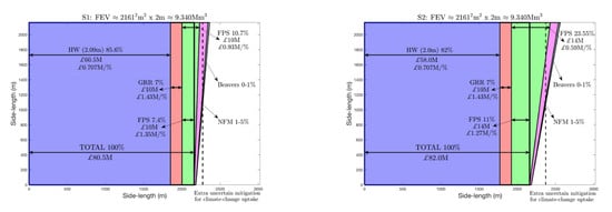
A visual comparison of the respective areas of each flood-mitigation measure S1 to S4 is found in Figure 10, where the width of each flood-mitigation measure portrays a relative contribution because each strip has the side length of the entire square flood lake of uniform depth. The strips are augmented by the percentages of each flood-mitigation measure as well as the total costs and costs per percentage gained. From Figure 9 and Figure 10, it becomes immediately clear that scenarios S0 and S4 are the cheapest. There are, however, some additional considerations to be taken into account. Scenario S0 does not reduce the required to update FASI to a 1:200-year return-period flood-event standard because the river water is not held back but, rather, flushed through the city of Leeds between higher flood-defence walls that quickly transport the floodwaters downstream. Significant floodwater storage as in scenario S4 lowers or may eliminate the need for updating FASI, the extent of which can best be assessed by further simulations of the flood hydraulics. Higher walls, such as those used in scenario S0, would protect only Leeds, whereas the enhanced flood-storage areas used in scenario S4 offer flood protection also further upstream, in other municipalities. Depending on the relative gains, it may be possible that it is advantageous to include the less cost-effective Rodley and Calverley storage sites as well (cf. Figure 11). Furthermore, calculation of FEVs at multiple spatial locations along the River Aire and similar cost-effectiveness analyses as given above may provide a more comprehensive view of the optimal and cost-effective flood-mitigation strategy over the entire river catchment upstream of and including Leeds. Finally, S1–S4 also provide additional extra mitigation against climate-change uplift, as indicated graphically.
The overall conclusion of our analysis of FASII is that our graphical presentation of the individual and overall effects of each flood-mitigation measure quantifies the reduction of the FEV, presented as a square flood lake of depth, directly combined with a cost-effectiveness analysis. It tentatively offers a novel assessment of flood-mitigation strategies that is simple to understand and to adapt, and which can therefore further assist policy makers in determining near-optimal flood-mitigation strategies.
4.3.2. Limitations of FEV-Based Approach
We are aware that the FEV approach offers a crude and imperfect assessment, to be used either prior to or in tandem with more detailed modelling studies when feasible. Such studies, however, not only take time but also cost money; by contrast, the FEV approach is one that invites exploration aimed at comparing a wide range of ideas rapidly, rather than aimed at an actual advanced risk-mitigation modelling approach. We outline some of its limitations:
- Zeroth-order approach: Three-dimensional flood dynamics is reduced to the analysis of FEV at or near the most critical point along a river where flooding starts. Generally river hydraulics are modelled in a one- or two-dimensional manner: it is therefore best to consider the zeroth-order FEV-analysis as a diagnostic at the worst spot.
- Retention: Only the averaged and cumulative effects of retention measures far upstream of the point of FEV-analysis are considered. Spatio-temporal considerations en route to the most critical point of flooding are thus ignored.
- Costs and effectiveness: Only effectiveness is considered here but not benefits, which would require a full economic analysis of damages saved and/or costs incurred, for example, for urban planning. In addition, maintenance aspects should be included more prominently.
Some of the above limitations can be overcome to some extent, as discussed next.
5. Summary and Discussion
To facilitate both the understanding of and comparison between extreme flooding events, we have revisited the concept of flood-excess volume (FEV), which is the product of the difference between the flood volume of river discharge and the discharge (associated with a certain critical river-level threshold ) with the flood duration. It is effectively the “area” under the flood hydrograph from upwards, cf. Figure 4. Since FEV is usually quantified in terms of millions of cubic metres, it is insightful to divide it by a depth of (a human-size scale with a choice of being too shallow and being too deep) and take the square root: one then gets a square lake of depth with the same capacity as the FEV. Such a flood-excess lake offers a better sense of the size of a flood and whether or not that lake fits within the relevant river valley either as one piece or divided into sub-lakes over the course of the river. FEV is exactly the effective volume one wishes to eliminate in order to prevent flooding because its elimination would ensure that the in-situ river level stays below the chosen critical threshold . Naturally there is variability of FEV with any chosen threshold , but the latter level can neither be too small, otherwise there is no flood (damage), nor can it be above the peak level of a flood event, since then FEV is by definition zero, that is, . To calculate FEV one generally must link measured river levels to discharge rates via rating curves; in so doing, one has to be careful because rating curves contain errors, which are often difficult to quantify. Several approximations for calculating rating curves, mean discharge and the FEV have been presented herein.
Subsequently, the FEV was estimated and calculated for the Boxing Day 2015 floods of the River Aire at Armley in Leeds, both in averaged and detailed ways. For the River Aire, the FEV was calculated to be or, equivalently, the capacity of a square -deep lake with a side-length of circa . The threshold of was carefully chosen as a flood threshold based on photographic and eyewitness evidence of the Boxing Day 2015 flood levels near Armley in combination with the river-level data measured.
FEV is insightful in analysing the relative importance of flood-mitigation measures proposed. Particularly useful is to address the following question: what fraction of the chosen FEV, that is, , is reduced by a particular flood-mitigation measure or policy? Flood-mitigation measures are assigned an associated (effective) volume capacity, which are then represented as pieces of a relevant square flood-excess lake. This provides a visualisation and interpretation that is comprehensible to both scientists and non-scientists, including policy makers, the public and flood practitioners. The corresponding costs of each flood-mitigation measure are presented in unison in our lake-based visualisation (see Figure 9 and Figure 10), alongside the respective fraction of each flood-mitigation measure, which leads to a visual cost-effectiveness analysis for facilitating decision-making.
To illuminate the FEV analysis, we have applied it to several hypothetical flood-alleviation scenarios (denoted by FASII), inspired by the existing Leeds’ Flood-Alleviation Scheme II (FASII), and have augmented it with cost and flood-storage-volume estimates seemingly absent from the public domain. FASII aims to provide flood protection against a flood event with a 1:200-year return period upstream of Leeds’ railway station and, in an extension of Flood-Alleviation Scheme I (FASI), of which construction finished in 2017 and which offers protection against a flood with a 1:100-year return period downstream of the Leeds’ railway station. Five FASII scenarios have been compared via a FEV cost-effectiveness analysis with flood-mitigation measures involving a combination of: flood-defence walls of various heights; a series of enhanced flood plains (at different locations and of different sizes); natural flood management, and; an update of FASI to a 1:200-year return-period flood. Such a FEV cost-effectiveness analysis provides a rational and advanced way to juxtapose and choose between flood-mitigation scenarios, in an understandable and quantitative manner. Scenario S4, of our hypothetical FASII, with its use of large storage volumes upstream of Leeds as well as some higher flood-defence walls in Leeds, was found to be most advantageous in terms of flood mitigation and cost. Scenario S4 will have additional benefits for communities upstream of the Leeds municipality and a minimal need to update FASI because floodwaters therein are partially held upstream of Leeds.
In all scenarios S1–S4 extra flood-plain storage was created by using dynamic weirs or sluice gates, to enhance and control the flood volume (see References [28,29]). A discovery that has been made explicit herein is that only the available flood-plain volume counts, a rarely recognised aspect in practice, which may not have been accounted for in FASII [21]. It is important to stress that the use of FEV does not replace the need for performing detailed model calculations in certain situations. It does, however, provide immediate guidance to refine such calculations a priori or, as an important practical alternative, replace such calculations in cases where insufficient computational resources are available.
Finally, there are several possible extensions of our analysis, listed as follows:
- FEV can be used to diagnose detailed hydraulic-flow calculations a posteriori; rather than using a measured flood hydrograph, one can first compute a reference-flood hydrograph and an associated FEV (or a range of such volumes for a range of thresholds), and then express calculations of scenarios with various flood-mitigation measures relative to this reference-flood hydrograph as () reductions of the associated FEV; such an approach can also be explored in a probabilistic manner by using ensemble calculations for a distribution of reference-flood hydrographs with different return periods, with FEVs calculated and compared at various critical spatial locations—see the roadmap in Section 4.1.1;
- FEV can be used as a complementary means of classifying flood events; flood hydrographs can be narrow, high and low-volume or broad, relatively high and high-volume, each with vastly different FEVs; for flood mitigation it is meaningful to reclassify return periods for river floods with sufficiently high peak levels in terms of FEV rather than in terms of only river-peak levels; and, this will be meaningful for only floods with peaks surpassing certain threshold levels ;
- FEV can play a central role in defining a new protocol to optimise the assessment of flood-mitigation scenarios, including a cost-effectiveness analysis; it may prove beneficial in certifying such a protocol in flood-mitigation handbooks. It is interesting to note that in 2019 a modified scenario S1 was chosen by LCC as flood-alleviation plan, including higher walls augmented with some wetland creation around Kirkstall, GRR between Kirkstall weir and the Dark Arches weirs at Leeds’ railroad station (cf. Figure 1) as well as enhanced dynamics flood-storage at Calverley [20]. NFM measures planned are expected to offer circa extra flood mitigation against climate-change uplift. Enhanced flood-plain storage far upstream of Leeds, cf. S4, has been dismissed; these have already provided some flood reduction for Leeds and upstream communities, cf. remarks in [30]. Enhanced storage at Rodley, close to Leeds, cf. scenarios S2 and S3, has been dismissed; the (formerly) optimal location for a dynamic weir at the narrow end of Rodley valley was moreover occupied by dwellings built in 2019.
- Finally, the square-lake cost-effectiveness protocol lends itself well to “gamification” [31,32], that is, integrating game elements into science education. This is recognised as a powerful way to engage and to inform those who may not be scientifically-literate, such as the general public and policy-makers, but nonetheless seek and would benefit from improved understanding. In particular, the concept and subsequent gamification of the so-called “stabilization wedges” [33] has proved successful in climate science. It is vital that both citizens and politicians understand how to “investigate, evaluate, and comprehend science content, processes, and products” [31], including flood-mitigation; inspired by the stabilization wedges, we intend to develop a game to communicate the efficacy and costs of various flood-mitigation scenarios, not only to inform the public but also to encourage evidence-based decision-making.
Author Contributions
O.B. developed the basic analysis and wrote the first drafts, which were critically reviewed, broken up, improved, adapted and rewritten by M.A.K., T.K., G.P. and J.-M.T.; T.K. also created and improved some of the figures and was a discussion partner since the Boxing Day flood of 2015 in Yorkshire. All authors have read and agreed to the published version of the manuscript.
Funding
This work grew out of EPSRC’s Living with Environmental Change (LWEC) UK network “Maths Foresees” (grant EP/M008525/1) as well as meetings within Sarah Dance’s EPSRC Data Science Fellowship “Data Assimilation for the REsilient City” (grant EP/P002331/1). The work of G.P. and J.-M.T. was funded by the H2020 project NAIAD [grant no. 730497] from the European Union’s Horizon 2020 research and innovation program.
Acknowledgments
We are indebted to the EA in Yorkshire for providing data of the Armley river gauge and information on rating curves. This article contains public sector information licensed under the Open Government Licence v3.0. A remark by Andy Moores of the EA within the network “Maths Foresees”, on flood plains already being partially occupied by floodwaters, led to our conceptualisation of available flood-plain or -storage volume.
Conflicts of Interest
The authors declare no conflict of interest.
Abbreviations
The following abbreviations are used in this manuscript:
| FEV | Flood-excess volume |
| EA | Environment Agency |
| UK | United Kindom |
| FASI | Leeds’ flood alleviation Scheme I |
| FASII | Leeds’ flood alleviation Scheme II |
| GRR | Giving-room-to-the-river |
| LCC | Leeds City Council |
| NFM | Natural Flood Management |
| HW | Higher walls |
| FPS | Flood-plain storage |
Appendix A. Propagation of Error Due to Rating-Curve Uncertainty
The summed approximation (2) is used to calculate the FEV of the Boxing Day flood at Armley gauge station as , a relative error of 16.1% (i.e., ). This error is due to, and propagates from, the uncertainty in the rating curve , and should be taken into account whenever the rating curve is applied in FEV calculations. To calculate the FEV error , we employ standard error-propagation techniques (cf. [34]) for multivariate nonlinear functions . Given uncorrelated errors , , the square of the error is
which is an approximation (using truncated series expansions) of the true (unknown) error and valid only for small . It is useful to recall and to rework the summed approximation (2):
with , , and ; the rating curve is used to calculate ( times), , and implicitly . For a function , summing over k and assuming uncorrelated errors and , the square of the error is given by (A1) as
in which the partial derivatives of can be readily derived from (A2) as
The rating-curve uncertainty for the Armley gauge station is reported as having a relative error of 5.5% so that and with . The missing component is thus , which cannot be expressed explicitly but can be approximated by computing for various values of given by the Armley gauge data, and then computing a (local) gradient at the value of chosen for the FEV calculation (see Figure A1). It follows that . It should be noted that, in this case, the error due to via is an order of magnitude smaller than that due to directly.
Figure A1.
Flood duration as an implicit function of threshold discharge, (black line), for the Boxing Day flood at Armley gauge station. The red line shows a linear approximation local to , the gradient of which is used to approximate in the FEV error calculation (A3). In this case, .
Figure A1.
Flood duration as an implicit function of threshold discharge, (black line), for the Boxing Day flood at Armley gauge station. The red line shows a linear approximation local to , the gradient of which is used to approximate in the FEV error calculation (A3). In this case, .

Appendix B. Bounds on Flood-Mitigation by Tree Planting
The River Aire catchment has approximate area , roughly aligned in a rectangle (see wikipedia). Trees are typically planted less than apart (see wikipedia), so trees cover an extra area of circa , which is indeed the aforementioned of tree coverage in the catchment area, cf. FASII’s NFM ([21], §3.2.3). NFM measures could be useful in protecting against flooding from less-severe flood events impacting infrastructure and dwellings further upstream of the proposed flood-mitigation measures in FASII, cf. [22]. Let us assume, as illustration, that estimated rainfall and peak-discharge increase due to climate change is circa .
Tree planting is most likely to occur in the upper catchment above Kildwick, in an area roughly a third of the total catchment area, such that (the extra) trees would thus cover about of it. Peak flows at Kildwick and Armley were respectively and , cf. Reference [9]. Assuming an upper-bound case by taking absorption of rainfall due to tree planting and uniform winter rainfall, trees would then reduce the peak flow at Kildwick by to about and at Armley to about ; these estimates are based on a linear scaling that can be improved by using the Kildwick and Armley river-gauge data. From Figure 8, it is clear that this upper bound on the discharge reduction via the tree-planting measure can at best only partially alleviate the FEV of because the relevant threshold discharge is (and the above rate of is still much higher). Hence, this would lead to an upper-bound estimate with reduction of the flood peak at Armley. In [22] it is reported that “In general, the strategy of “retaining water in the landscape” through decentralised measures such as afforestation, small-reservoirs and micro-ponds could play an important role for flood management in meso-scale catchments for small and medium events, but has almost negligible effects during the largest flood events” and continue to highlight co-benefits. Our argument above is a reductio ad absurdum: while the upper bound of reduction by tree planting is small, its contribution becomes much smaller when the unrealistic assumption of rainwater absorption is replaced to lie in a range from to , say, since absorption is often insignificant for the large flood events, cf. [22]. Hence, given both that an upper bound on the water absorption was used and the uncertainties surrounding NFM’s effectiveness for extreme rainfall events, we have used this NFM measure only to (partially) offset increased run-off due to climate change. LCC’s original FASII plans of December 2017 are clear about the role of NFM in mitigating climate-change effects only, but only because no quantification of its effectiveness is provided (i.e., it was safely set to ). By contrast, there is a clear quantification of flood protection against a 1:200-year return-period flood for the cases in Table 3 involving flood-defence walls. Perhaps due to our analysis and critique [15], the contribution of NFM in Leeds FASII’ 2018 update has been corrected, since the update now includes both tree planting as well as leaky dams, and an estimated flood mitigation of (this maximum of was communicated to us in person at a public consultation with Leeds City Council in early 2019). We have set the (to-date-unknown) uncertainty of NFM to for illustrative purposes, cf. [22].
References
- Sanderson, M. 2010: Changes in the Frequency of Extreme Rainfall Events for Selected Towns and Cities. Met Office “Ofwat” Report. Available online: https://www.ofwat.gov.uk/wp-content/uploads/2015/11/rpt_com_met_rainfall.pdf (accessed on 26 February 2020).
- Stocker, T.F.; Qin, D.; Plattner, G.-K.; Tignor, M.; Allen, S.K.; Boschung, J.; Nauels, A.; Xia, Y.; Bex, V.; Midgley, P.M. (Eds.) IPCC 2013: Summary for Policymakers. In Climate Change 2013: The Physical Science Basis. Contribution of Working Group I to the Fifth Assessment Report of the Intergovernmental Panel on Climate Change; Cambridge University Press: Cambridge, UK; New York, NY, USA, 2013. [Google Scholar]
- Environment Agency 2018: The Costs of the Winter 2015 to 2016 Floods. Summary at: https://www.gov.uk/government/uploads/system/uploads/attachment_data/file/672088/costs_of_the_winter_floods_2015_to_2016_summary.pdf (accessed on 26 February 2020). Available online: https://www.gov.uk/government/uploads/system/uploads/attachment_data/file/672087/Estimating_the_economic_costs_of_the_winter_floods_2015_to_2016.pdf (accessed on 26 February 2020).
- Kron, W.; Eichner, J.; Kundzewicz, Z.W. Reduction of flood risk in Europe –Reflections from a reinsurance perspective. J. Hydrol. 2019, 576, 197–209. [Google Scholar] [CrossRef]
- Kundzewics, Z.W.; Hegger, D.L.T.; Matczak, P.; Driessen, P.P.J. Flood risk reduction: Structural measures and diverse strategies. Proc. Natl. Acad. Sci. USA 2018, 115, 12321–12325. [Google Scholar] [CrossRef] [PubMed] [Green Version]
- Santoro, S.; Pluchinotta, I.; Pagano, A.; Pengal, P.; Cokan, B.; Giordano, R. Assessing stakeholders’ risk perception to promote Nature Based Solutions as flood protection strategies: The case of the Glinščica river (Slovenia). Sci. Total Environ. 2019, 665, 188–201. [Google Scholar] [CrossRef] [PubMed]
- Pagano, A.; Pluchinotta, I.; Pengal, P.; Cokan, B.; Giordano, R. Engaging stakeholders in the assessment of NBS effectiveness in flood risk reduction: A participatory System Dynamics Model for benefits and co-benefits evaluation. Sci. Total Environ. 2019, 690, 543–555. [Google Scholar] [CrossRef] [PubMed]
- Guardian UK News 2015: Severe Flooding in Britain Prompts Boxing Day Evacuations—As It Happened. Available online: https://www.theguardian.com/environment/live/2015/dec/26/severe-flood-warnings-in-the-north-prompt-boxing-day-evacuation-fears (accessed on 26 February 2020).
- Environment Agency 2016a: Hydrology of the December 2015 Flood in Yorkshire. April 2016 Report of Environment Agency. Available online: https://www.ceh.ac.uk/sites/default/files/2015-2016%20Winter%20Floods%20report%20Low%20Res.pdf (accessed on 26 February 2020).
- West Yorkshire Combined Authority 2016: Leeds City Region Flood Review Report—December 2016. Available online: https://www.the-lep.com/media/2276/leeds-city-region-flood-review-report-final.pdf (accessed on 26 February 2020).
- Akers, B.; Bokhove, O. Hydraulic flow through a contraction: Multiple steady states. Phys. Fluids 2008, 20, 056601. [Google Scholar] [CrossRef] [Green Version]
- Hankin, B.; Arnott, S.; Whiteman, M.; Burgess-Gamble, L.; Rose, S. Working with Natural Processes—Using the Evidence Base to Make the Case for Natural Flood Management. Environment Agency Report. 2017. Available online: https://www.gov.uk/government/uploads/system/uploads/attachment_data/file/654435/Working_with_natural_processes_using_the_evidence_base.pdf (accessed on 26 February 2020).
- Hui, R.; Lund, J.R. Flood Storage Allocation Rules for Parallel Reservoirs. J. Water Res. Plan. Manag. 2014, 141, 469. [Google Scholar] [CrossRef] [Green Version]
- Environment Agency. River Aire at Armley, Rating Change Report August; Environment Agency: Bristol, UK, 2016.
- Bokhove, O.; Kelmanson, M.A.; Kent, T. On Using Flood-Excess Volume in Flood Mitigation, Exemplified for the River Aire Boxing Day Flood of 2015. 2018. Available online: https://eartharxiv.org/stc7r/ (accessed on 26 February 2020).
- Perks, M. Non-Contact Monitoring—Why Use a Non-Contact Monitoring Approach? 2019. Available online: https://flood-obs.com/non-contact-monitoring/ (accessed on 26 February 2020).
- Bokhove, O.; Kelmanson, M.A.; Kent, T. On Using Flood-Excess Volume to Assess Natural Flood Management, Exemplified for Extreme 2007 and 2015 Floods in Yorkshire. 2018. Available online: https://eartharxiv.org/87z6w/ (accessed on 26 February 2020).
- Bokhove, O.; Kelmanson, M.A.; Kent, T.; Piton, G.; Tacnet, J.-M. Communicating (nature-based) flood-mitigation schemes using flood-excess volume. River Res. Appl. 2019, 35, 1402–1414. [Google Scholar] [CrossRef] [Green Version]
- Guardian UK News. Three Dead and 1000 Evacuated as Floods Strike. 2007. Available online: https://www.theguardian.com/uk/2007/jun/26/topstories3.weather (accessed on 26 February 2020).
- Leeds City Council. Leeds Flood-Alleviation Scheme Phase II. 2019. Available online: https://www.leeds.gov.uk/parking-roads-and-travel/flood-alleviation-scheme/flood-alleviation-scheme-phase-two (accessed on 26 February 2020).
- Leeds Executive Board. Decision Details—Phase 2 Leeds (River Aire) Flood Alleviation Scheme. Documents. 2017. Available online: http://democracy.leeds.gov.uk/ieDecisionDetails.aspx?ID=45047 (accessed on 26 February 2020).
- Salazar, S.; Francés, F.; Komma, J.; Blume, T.; Francke, T.; Bronstert, A.; Blöschl, G. A comparative analysis of the effectiveness of flood management measures based on the concept of “retaining water in the landscape” in different European hydro-climatic regions. Nat. Hazards Earth Syst. Sci. 2012, 12, 3287–3306. [Google Scholar] [CrossRef] [Green Version]
- Puttock, A.; Graham, H.A.; Cunliff, A.M.; Elliott, M.; Brazier, R.E. Eurasian beaver activity increases water storage, attenuates flow and migrates diffuse pollution from intensively-managed grasslands. Sci. Total Environ. 2017, 576, 430–443. [Google Scholar] [CrossRef] [PubMed] [Green Version]
- BBC News. Beaver Experiment ‘to Combat Flooding’ in North Yorkshire. 2018. Available online: https://www.bbc.co.uk/news/uk-england-york-north-yorkshire-45708504 (accessed on 26 February 2020).
- BBC News. Beavers to be reintroduced in Somerset and South Downs. 2019. Available online: https://www.bbc.co.uk/news/uk-england-somerset-50485784 (accessed on 26 February 2020).
- Guardian UK News. Beavers to be Released in Plan to Ease Flooding and Aid Biodiversity. 2019. Available online: https://www.theguardian.com/environment/2019/nov/20/beavers-to-be-released-in-plan-to-ease-flooding-and-aid-biodiversity (accessed on 26 February 2020).
- Environment Agency. Press Release: £50 Million Flood Defence Scheme Opens in Leeds. 2017. Available online: https://www.gov.uk/government/news/50-million-flood-defence-scheme-opens-in-leeds (accessed on 26 February 2020).
- Breckpot, M. Flood Control of River System with Model Predictive Control; the River Demer as a Case Study. Ph.D. Thesis, KU Leuven, Leuven, Belgium, 2013. [Google Scholar]
- Breckpot, M.; Agudelo, O.M.; De Moor, B. Flood control with Model Predictive Control for river systems with water reservoirs. J. Irrig. Drain. Eng. 2013, 139, 532–541. [Google Scholar] [CrossRef]
- NRFA. Aire at Armley—Station Info. See Flow regime description: “...Washlands Created at Skipton and Silsden to Manage Flooding at Leeds”. 2019. Available online: https://nrfa.ceh.ac.uk/data/station/info/27028 (accessed on 26 February 2020).
- Morris, B.; Croker, S.; Zimmerman, C.; Gill, D.; Romig, C. Gaming science: The “Gamification” of scientific thinking. Front. Psychol. 2013, 4, 607. [Google Scholar] [CrossRef] [Green Version]
- Bowser, A.; Hansen, D.; He, Y.; Boston, C.; Reid, M.; Gunnell, L.; Preece, J. Using gamification to inspire new citizen science volunteers. In Proceedings of the First International Conference on Gameful Design, Research, and Applications, Toronto, ON, Canada, 2–4 October 2013. [Google Scholar]
- Pacala, S.; Socolow, R. Stabilization wedges: Solving the climate problem for the next 50 years with current technologies. Science 2004, 305, 968–972. [Google Scholar] [CrossRef] [PubMed] [Green Version]
- Priestley, M.B. Spectral Analysis and Time Series; Academic Press: London, UK; New York, NY, USA, 1981; 890p. [Google Scholar]
Figure 1.
Environment Agency (EA) flood-risk maps of the sectors Kildwick (top left in upper map) to Apperley Bridge (yellow marker in both maps) and Apperley Bridge to Leeds (bottom right in lower map). Available online at https://flood-map-for-planning.service.gov.uk, for example, search (easting, northing) = (419,052, 437,681) for Apperley Bridge. Extra flood storage may be available at locations 1, 2, 3 and 4 on the lower map, respectively corresponding to the top-left, top-right, bottom-left and bottom-right photographs in Figure 11.

Figure 2.
Boxing Day 2015 flooding levels of the River Aire near Apperley Bridge (river near the yellow marker in Figure 1; the old bridge just upstream of the modern A658-road bridge). Top: the filled flood plain upstream of the bridge constriction at 09:56:04 on 26 December 2015. Bottom: the flow under Apperley Bridge at circa 09:58:30 on the same date, showing the dangerous proximity to choking, akin to experiments in [11]. Photo and video-grab courtesy of O.B.

Figure 3.
Top left: plaques at Leeds’ Armley Mills Museum indicate 1866 and 2015 flood-peak levels, the latter associated with the peak level of m at the Armley river-level gauge. Craig Duguid (Fluid Dynamics’ Centre for Doctoral Training, Leeds) provides a sense of scale. Top right: high level and supercritical flow in the “Dark Arches” underneath Leeds railway station at 13:36:04 on 27 December 2015; the high-water mark on the wall outlines the peak level, at 13:36:36 on 27 December 2015. Bottom left: subcritical flow emanating from these arches at 13:29:42 on 27 December 2015. Bottom right: entrance and top of the weir at these arches on 19 February 2018 with subcritical inflow. Photos and video-grabs courtesy of O.B.

Figure 4.
The rating curve including errors (solid line, top-left panel) and its linear approximation (dashed line) are displayed as well as river levels (lower-left panel) and peak-flow rates including errors (top-right panel) of the River Aire at Armley, Leeds, around Boxing Day 2015. Dotted lines indicate a chosen threshold, the corresponding discharge and a mean river level. The flood-excess volume (FEV) is found by determining the blue-shaded “area”, as in (2), under the discharge curve displayed on the vertical axis as a function of time t on the horizontal axis. It involves the in-situ river level as a function of time t above a threshold discharge . Given a rating curve, is fixed once a chosen threshold river level, here , has been provided. The flood duration for threshold is . The rectangle represents the mean FEV, with the hatched “area” defined in (3). The dashed-line correction to the rating curve concerns giving-room-to-the-river (GRR) or river-bed widening. It leads to a higher threshold with a reduced FEV for the same river-level threshold . The grey shading denotes the error in Q due to rating-curve uncertainty (not shown for the GRR curve). Data from EA.

Figure 5.
Flooding starts at Kirkstall on 26 December 2015 at 12:18 with the Armley river level recorded at m, which motivates one to take a threshold river level at . Photo courtesy Jessica Worsey.
Figure 5.
Flooding starts at Kirkstall on 26 December 2015 at 12:18 with the Armley river level recorded at m, which motivates one to take a threshold river level at . Photo courtesy Jessica Worsey.

Figure 6.
By using Gaugemap (http://www.gaugemap.co.uk) at the Armley station, one can quickly estimate the river level of the mean area indicated by the top rectangle above , which yields a mean height at the arrow of about ; by using the online time slider, one can also also find the duration for which the flood level was above .

Figure 7.
River Aire levels at Armley, Leeds, from May 2015 until the end of March 2016. EA data.

Figure 8.
River Aire flood-excess volumes (left axis, crosses) and equivalent square-lake sizes (right axis, circles) for various threshold levels , from the Armley data of the Boxing Day 2015 flood.
Figure 8.
River Aire flood-excess volumes (left axis, crosses) and equivalent square-lake sizes (right axis, circles) for various threshold levels , from the Armley data of the Boxing Day 2015 flood.

Figure 9.
Top: FEV expressed as a square -deep lake of side-length 2161 m. Bottom: the FEV lake, shallow relative to its side length, viewed from the top. Basic scenario S0 is depicted with higher flood-defence walls and National Flood Management (NFM) giving respectively and protection (see Appendix B) against the desired 1:200-year return-period flood event. Indicated in the square lake are the relative size of each flood-mitigation measure, expressed both as lake area and the length of double-ended arrows, and its costs in UK pounds sterling. Split and total costs are indicated in absolute terms and per percentage of the total flood mitigation gained. Total costs (excluding NFM), here equalling the protection offered by using only higher flood-defence walls, are indicated underneath the double-ended arrow spanning the width of the entire flood lake.

Figure 10.
Scenarios S1 to S4 with contribution of each flood-mitigation measure proportional to the length of the (inverted) double-headed arrows. Contributions to the square flood-excess lake (of the same capacity as the FEV) are: higher walls with wall-heights indicated (HW—mauve); river-bed widening (GRR—red); and (enhanced) flood-plain storage (FPS—green). The uncertain, slanted parts of FPS, natural flood management (NFM—pink) and beaver colonies (small sliver—blue) are used as extra flood mitigation to offset climate-change effects, beyond the 2161 side, with the mean denoted as the vertical dashed line. Above or alongside the double arrow the total percentage of protection for each flood-mitigation measure is given; below the double arrow costs and relative cost per of flood mitigation are stated. Total costs are indicated under the double arrow spanning the lake width.


Figure 11.
Evidence of extra/limited storage capacity above and beyond the Boxing Day 2015 flood levels for the River Aire; 1. top left: extra storage capacity downstream of Apperley Bridge both upstream of the Victorian railway bridge and downstream (26 December 2015 at 15:27:33); 2. top right: no extra storage capacity at Kirkstall Forge, where a shallow cut has been added to the sharp bend to alleviate flood risk on the visible train tracks; 3. bottom left: extra storage on the Rodley nature reserve flood plain (27 December 2015 at 12:15:05); and, 4. bottom right: downtown flooding just upstream of the station where the Leeds-Liverpool canal could be used as bypass of the “Dark Arches” hydraulic control point under Leeds’ train station (27 December 2015 at circa 13:20:53), shown in Figure 3. Photos and video-grab courtesy of O.B.


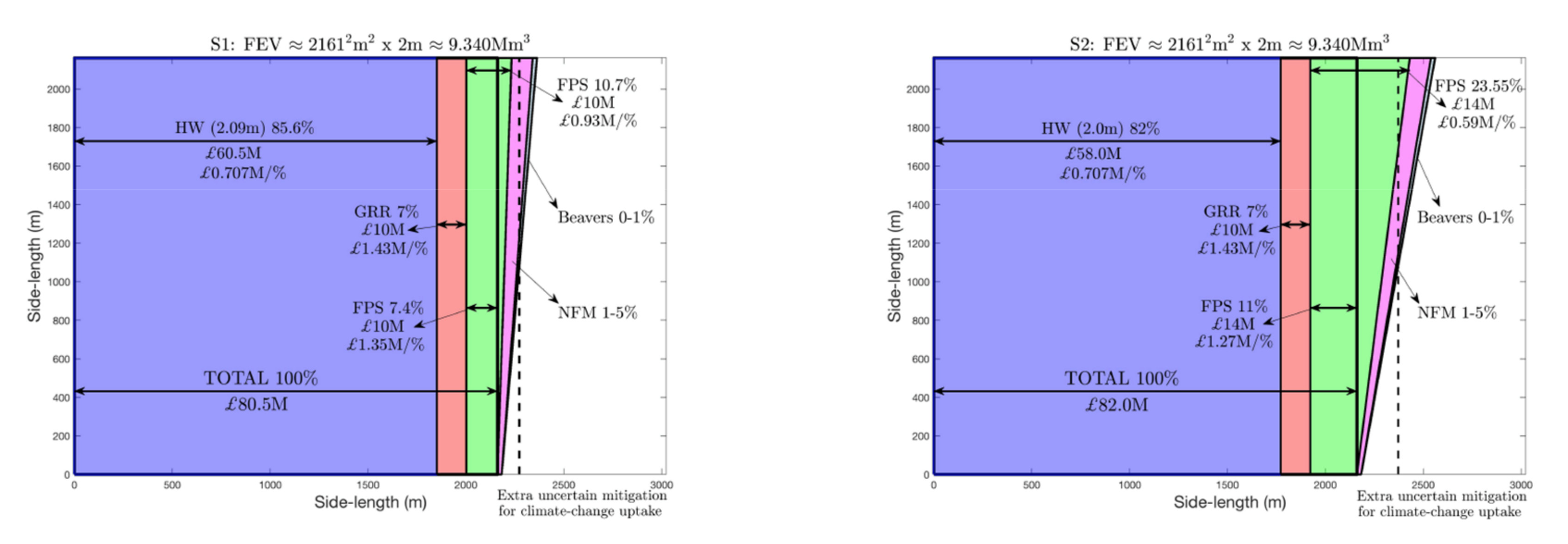
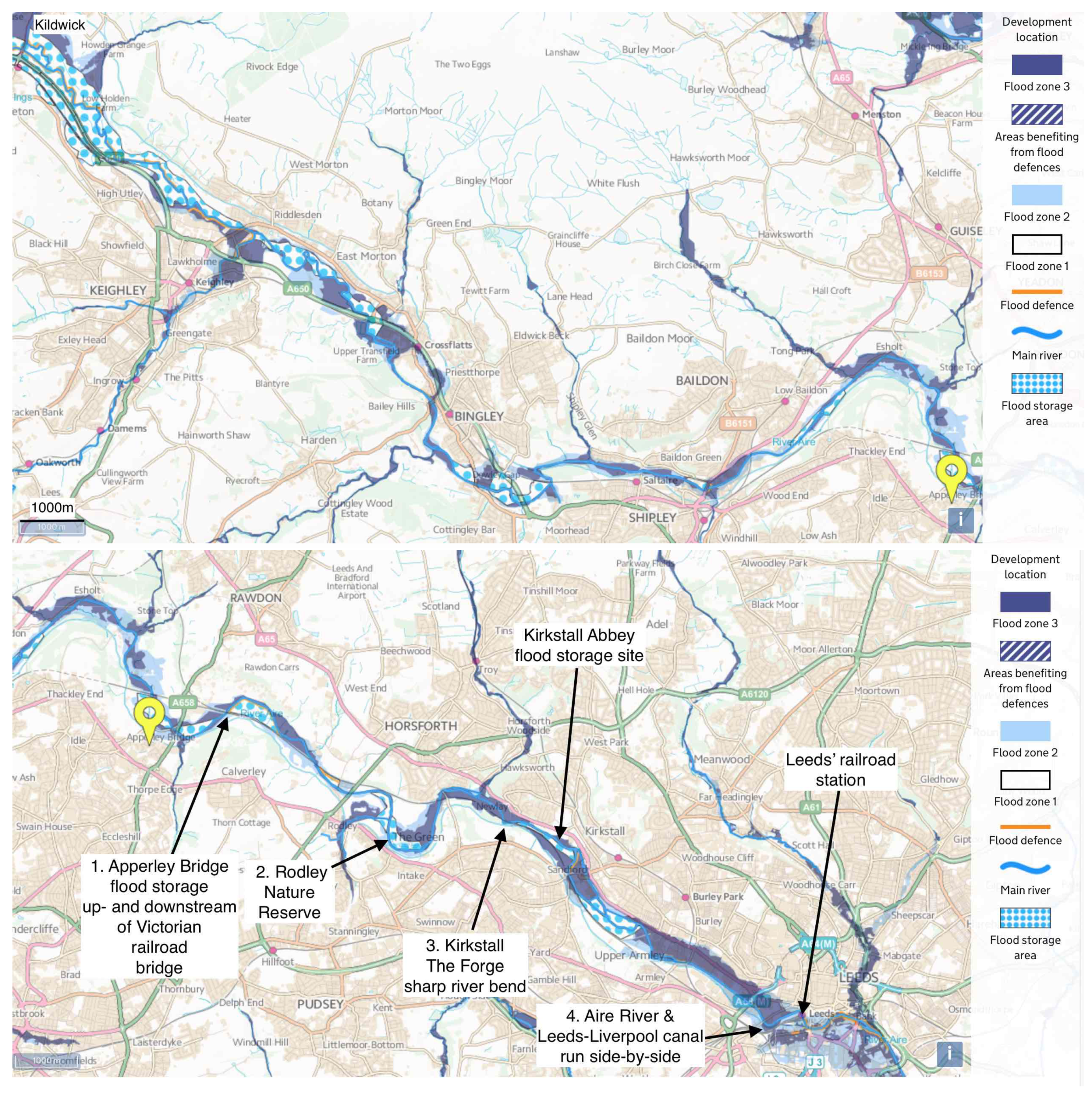
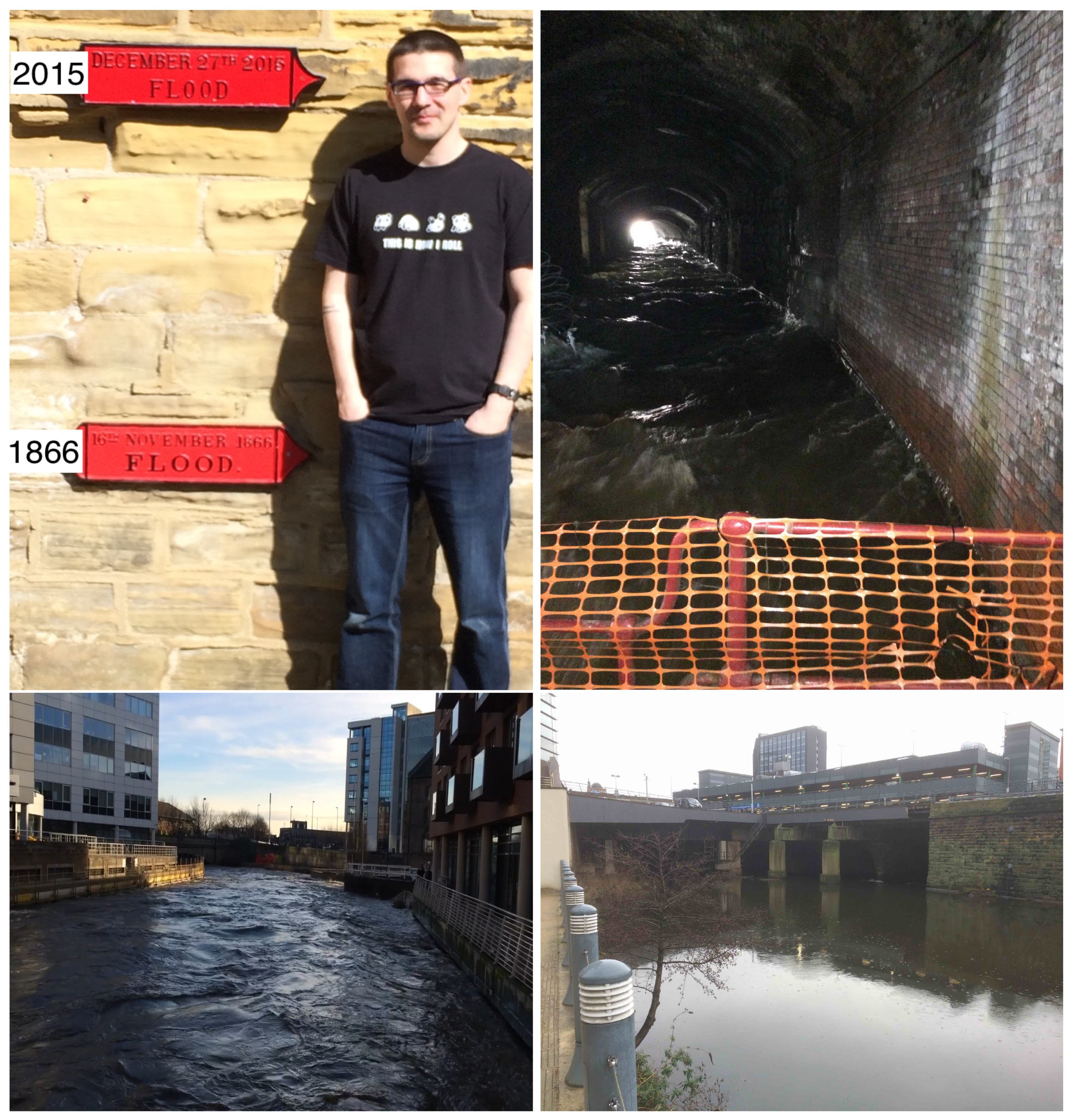
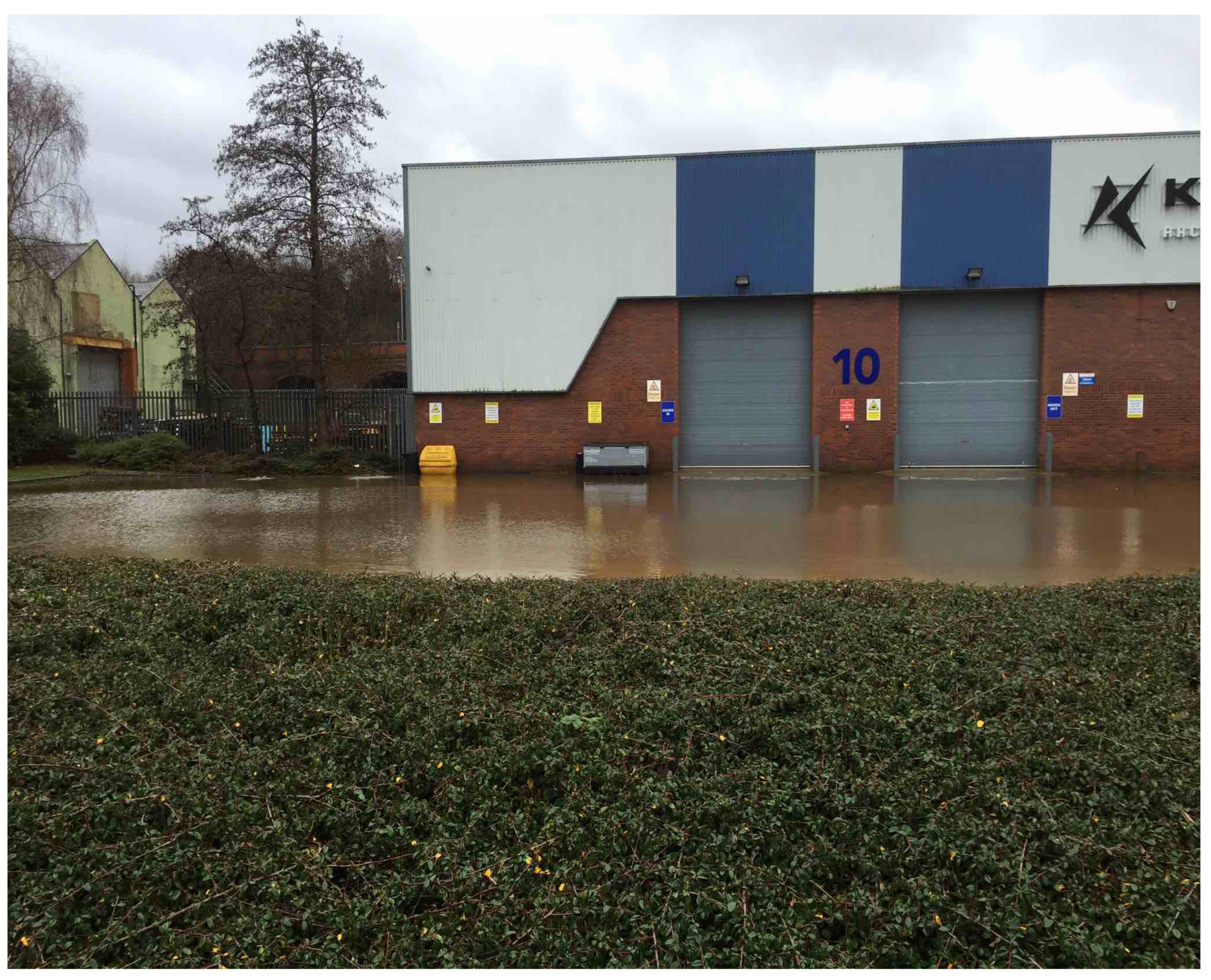
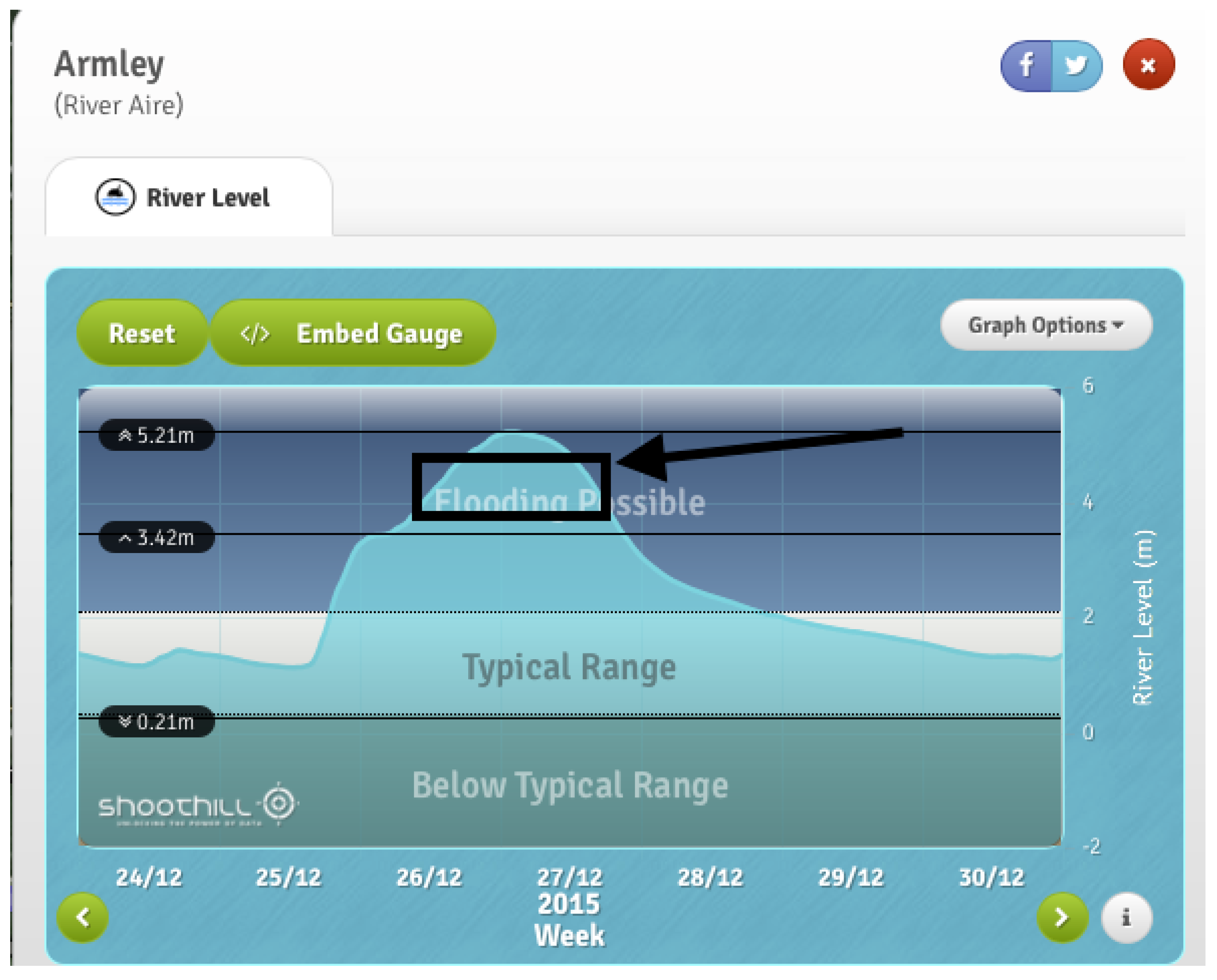
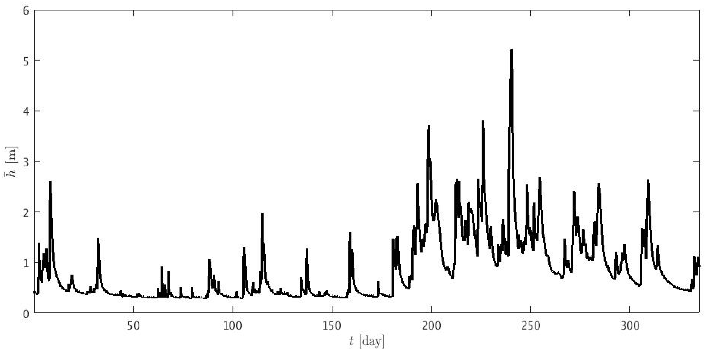
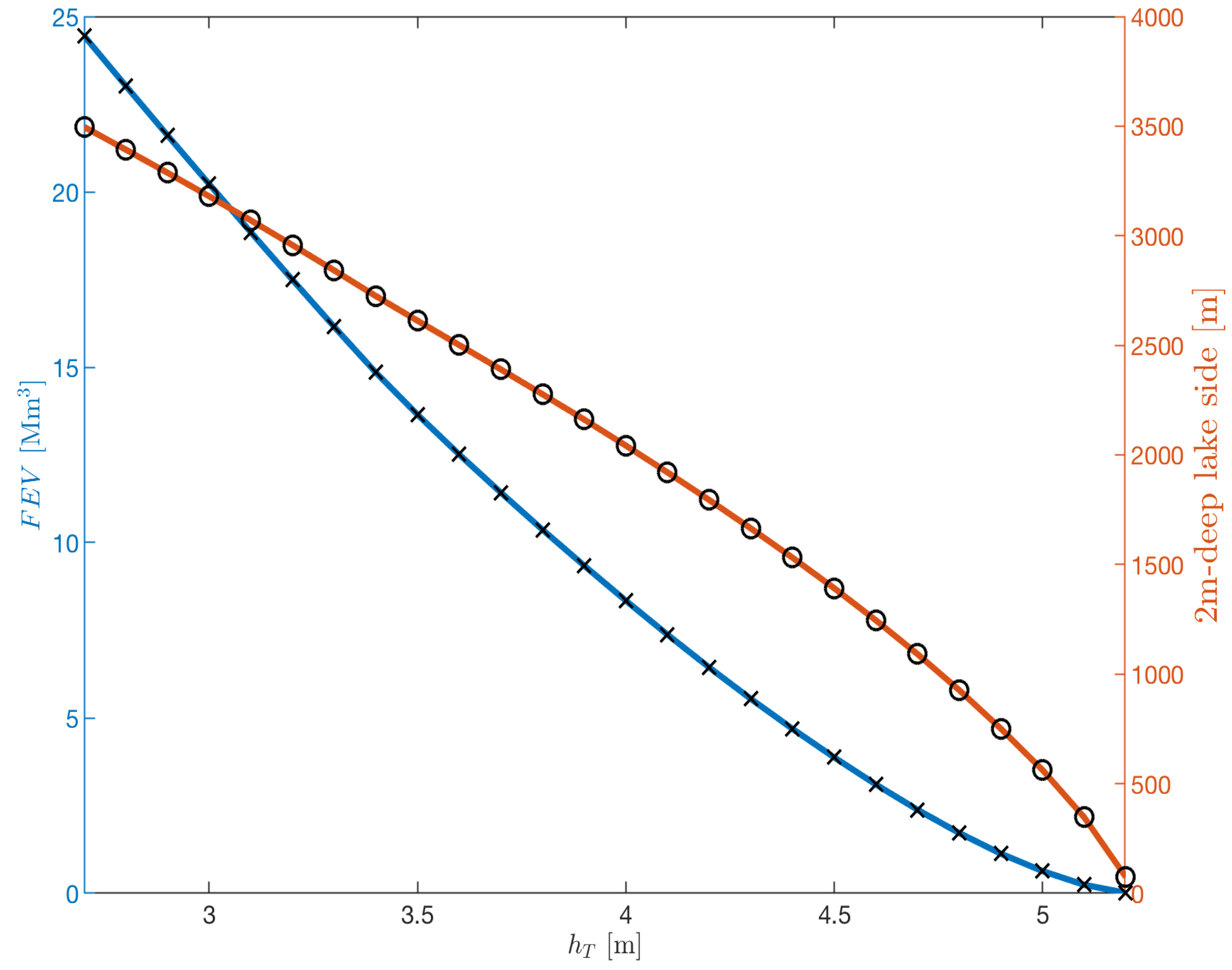
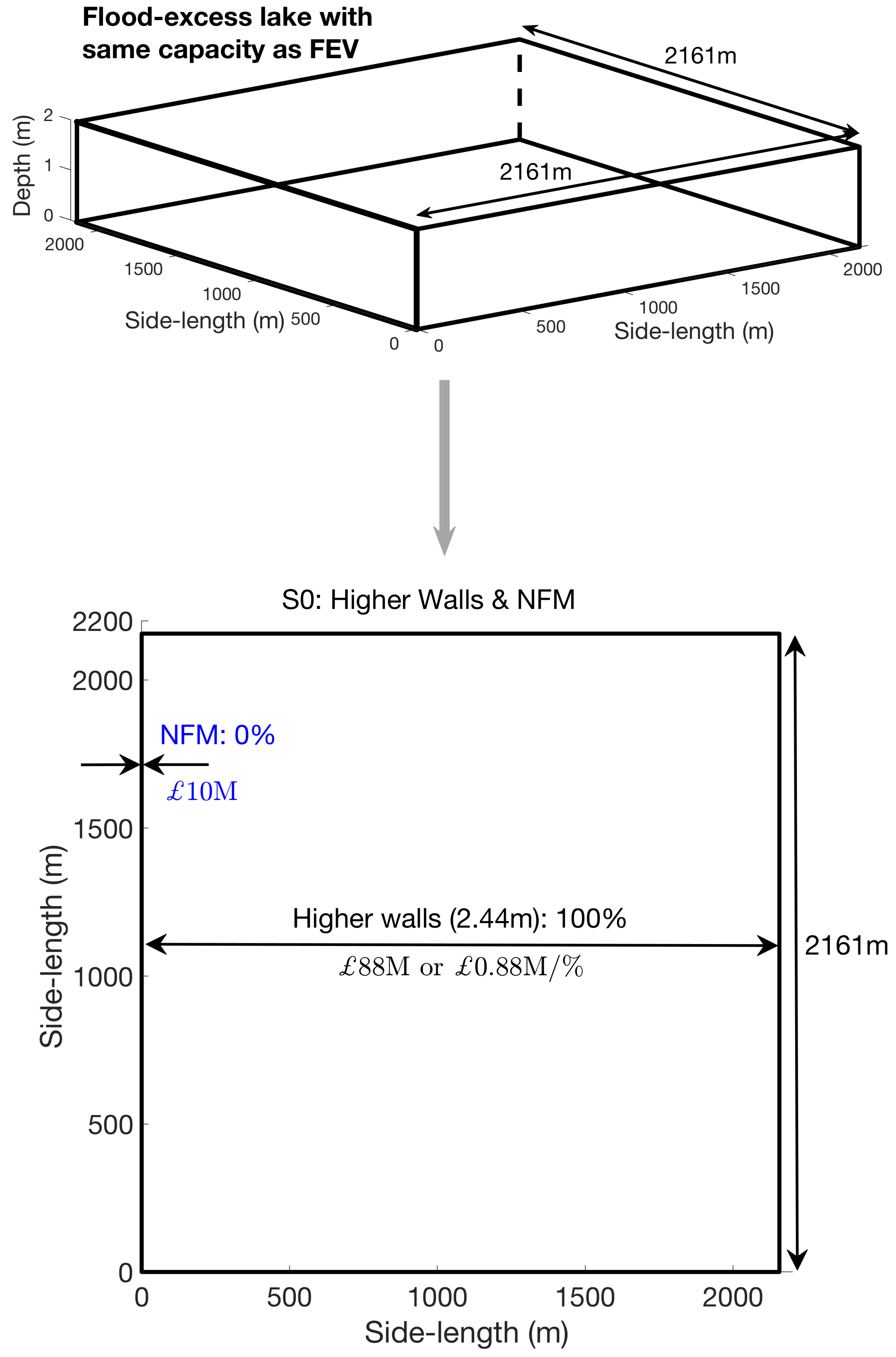
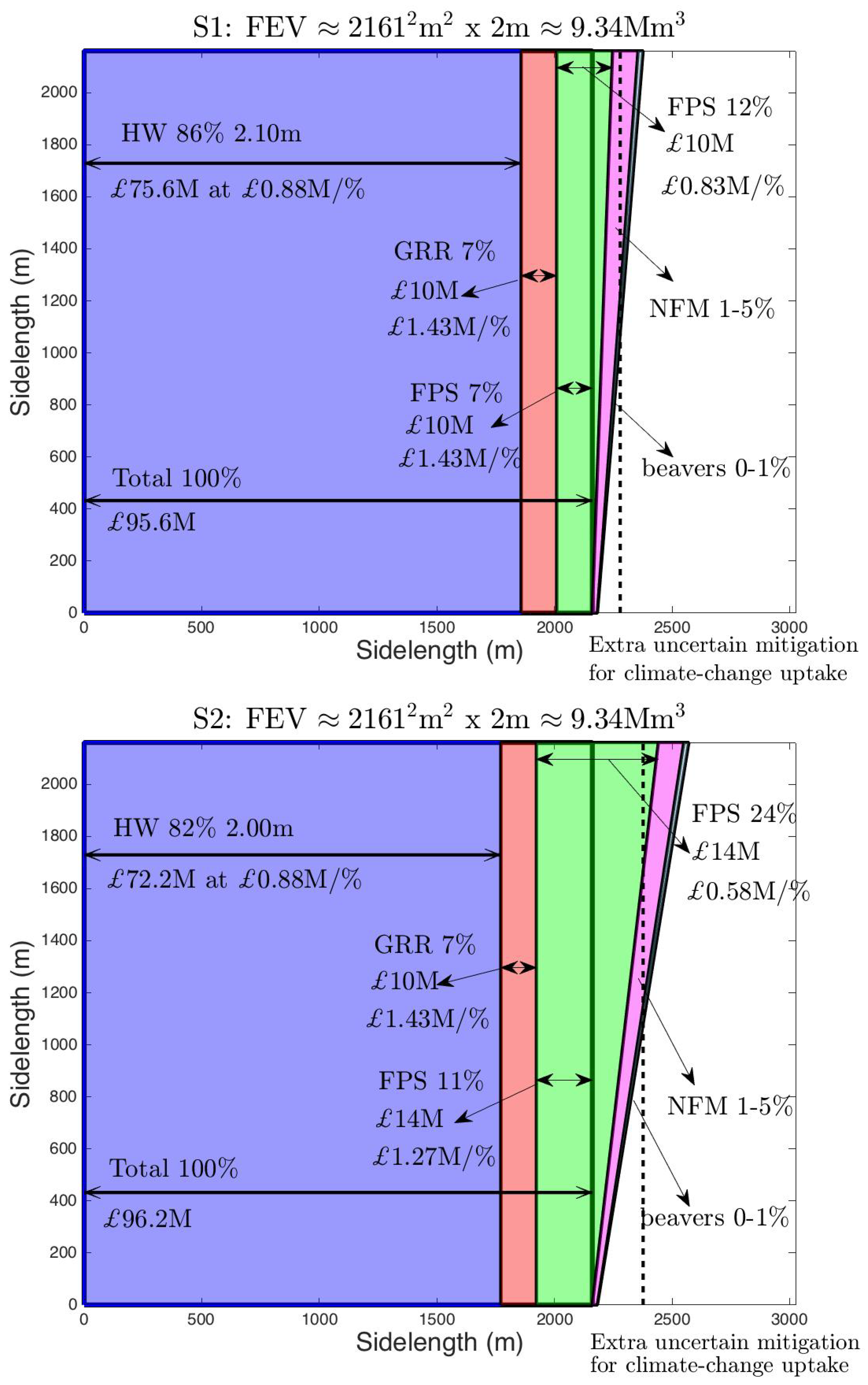
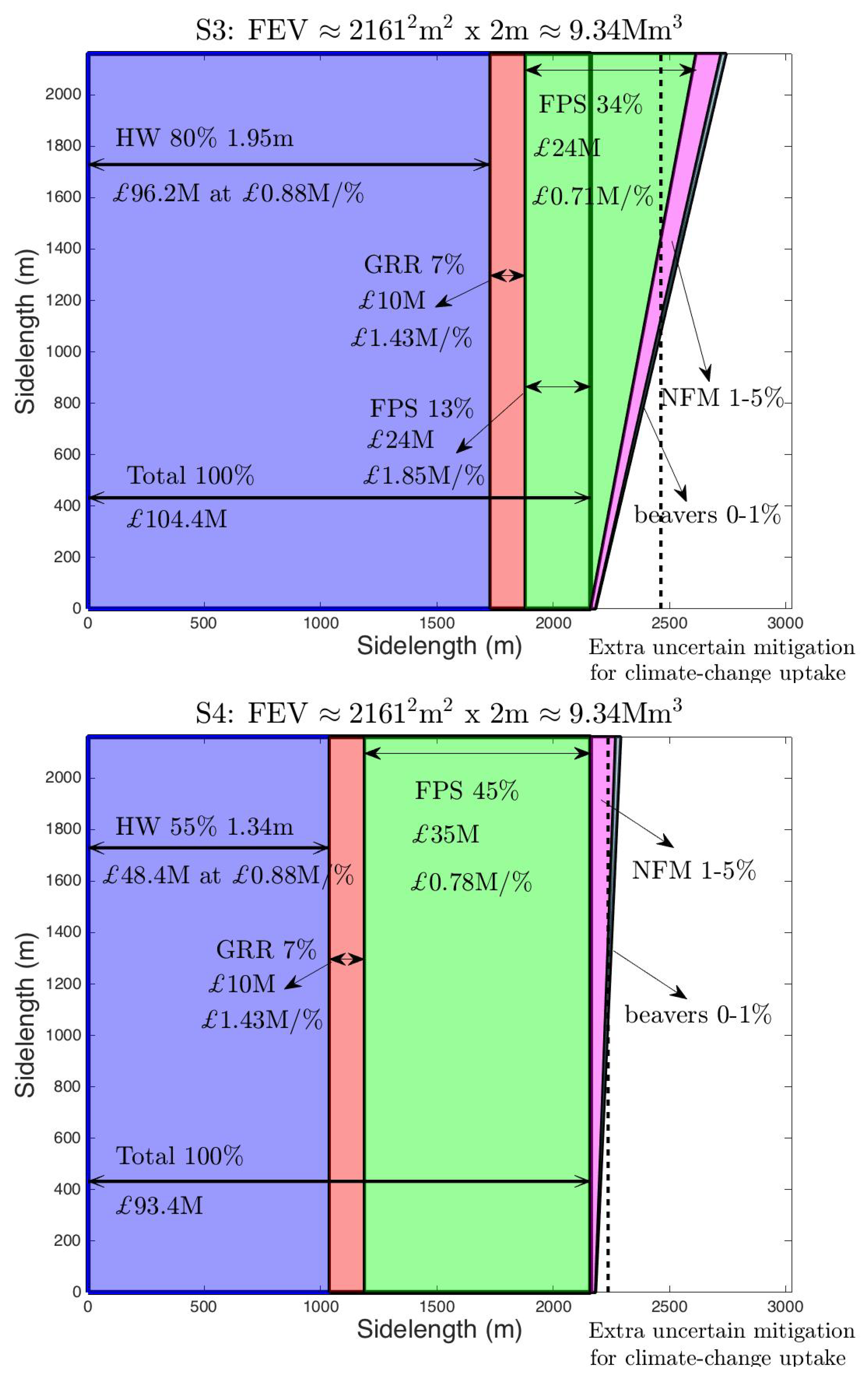
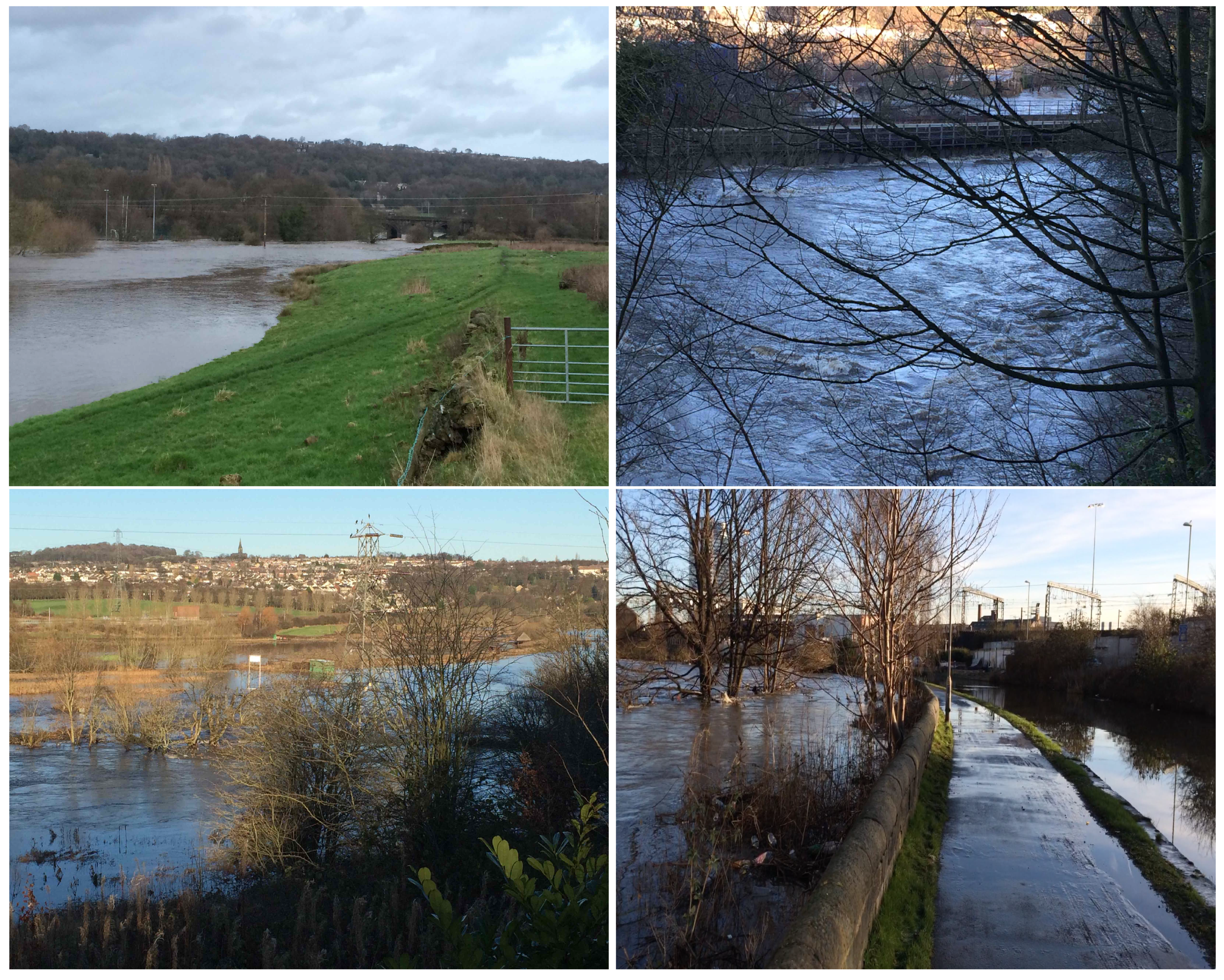
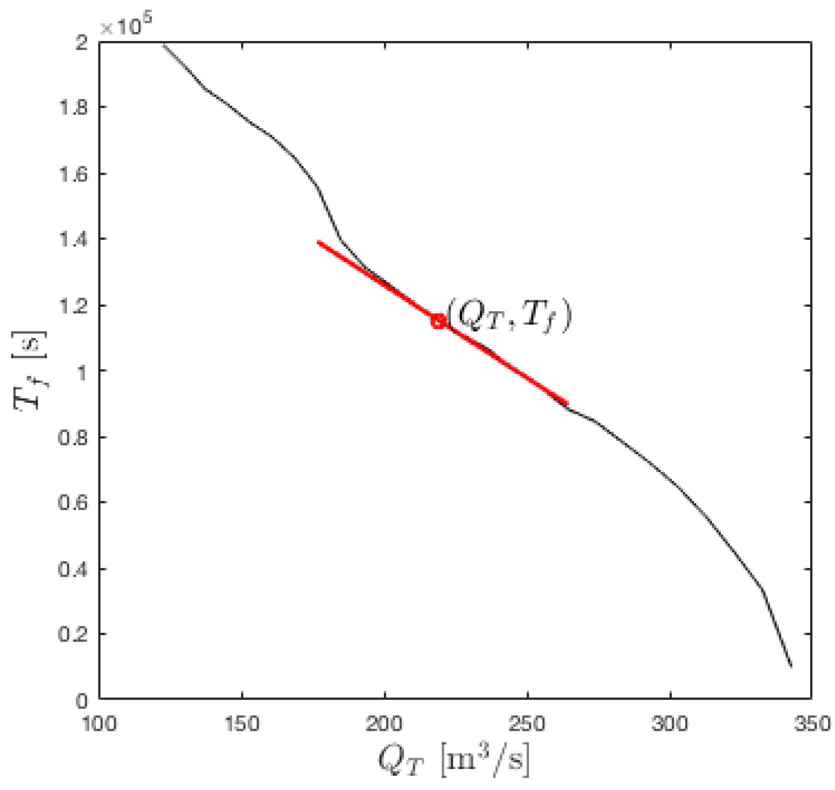
Table 1.
The latest [14] coefficients and limb thresholds and for for the rating curve at the river-level gauge station at Armley in Leeds.
Table 1.
The latest [14] coefficients and limb thresholds and for for the rating curve at the river-level gauge station at Armley in Leeds.
| j | ||||
|---|---|---|---|---|
| - | ||||
| 1 | 0.685 | 30.69 | 0.156 | 1.115 |
| 2 | 1.917 | 27.884 | 0.028 | 1.462 |
| 3 | 4.17 | 30.127 | 0.153 | 1.502 |
Table 2.
Hypothetical flood-alleviation scheme FASII: a summary of the various protection measures, their function (qualitative) and capacity (quantitative), and in which scenarios (S0–S4) they feature. A detailed description of each component is given in Section 4.1, Section 4.2 and Section 4.3.
Table 2.
Hypothetical flood-alleviation scheme FASII: a summary of the various protection measures, their function (qualitative) and capacity (quantitative), and in which scenarios (S0–S4) they feature. A detailed description of each component is given in Section 4.1, Section 4.2 and Section 4.3.
| Measure | Function | Capacity | S0 | S1 | S2 | S3 | S4 |
|---|---|---|---|---|---|---|---|
| Flood walls | Increase local flow capacity (effectively increasing ) | Various (depending on scenario), see Table 3 | X | X | X | X | X |
| NFM: Natural flood management | Store water in the catchment headwaters | Leaky dams & increase tree coverage by 8% | X | X | X | X | X |
| GRR: Giving-room-to- the-river | Increase local flow capacity (by river-bed widening & removing constrictions) | X | X | X | X | ||
| Beavers | Store water in the catchment headwaters | 85 beaver colonies storing each | X | X | X | X | |
| Calverley site | Flood-plain storage | Total: . Available: . | X | X | |||
| Rodley site | Flood-plain storage | Total: . Available: . | X | X | |||
| Cononley Washlands & Holden Park sites | Flood-plain storage | X |
Table 3.
The height of the defence walls proposed in FASII for protection against the 1:200-year flood and height reduction in percentage, along two different river stretches for the cases with only walls, walls with also the Rodley flood storage, or also the Apperley Railway Bridge/Calverley storage, or both. The wall-height reduction is given as a percentage for each location and can be compared against the extra flood-storage reduction percentage with respect to the flood excess volume (FEV) of chosen. Percentages relative to are calculated by us, with an adjustment by a factor added in parentheses giving the percentage relative to , and wall heights are from a table in [21] based on Leeds City Council’s (LCC’s) calculations/simulations. The underlined percentages are used in FASII.
| Location | Walls Only | Walls Plus Rodley | Walls Plus Calverley | Walls Plus Rodley & Calverley |
|---|---|---|---|---|
| Whitehall Rd to Wellington Br | 1.74 m | 1.53 m | 1.60 m | 1.50 m |
| - | −12% (−11%) | −8% (−7%) | −14% (−13%) | |
| Viaduct Rd to Cardigan Fields | 2.27 m | 2.00 m | 2.09 m | 1.96 m |
| - | −12% (−11%) | −8% (−7%) | −14% (−13%) | |
| Reduction of FEV by upstream retention | ||||
| ( |
Table 4.
Table summarising the figures for the five scenarios S0, S1–S4 of FASII; total costs for FPS (minimum case) are minus the FASI improvements needed, which were costed at for scenario S1. Tentative wall heights are for the stretch including Viaduct Road, cf. Table 3.
Table 4.
Table summarising the figures for the five scenarios S0, S1–S4 of FASII; total costs for FPS (minimum case) are minus the FASI improvements needed, which were costed at for scenario S1. Tentative wall heights are for the stretch including Viaduct Road, cf. Table 3.
| GRR % | FPS % | min | Case | HW % | m | FPS % | Max | Case | Total | |||||
|---|---|---|---|---|---|---|---|---|---|---|---|---|---|---|
| S0 | 0 | - | - | 0 | - | - | 100 | 88 | 0 | - | - | 88 | ||
| S1 | 7 | 10 | 7 | 10 | 86 | 12 | 10 | |||||||
| S2 | 7 | 10 | 11 | 14 | 82 | 24 | 14 | |||||||
| S3 | 7 | 10 | 13 | 24 | 80 | 34 | 24 | |||||||
| S4 | 7 | 10 | 45 | 35 | 55 | 45 | 35 |
© 2020 by the authors. Licensee MDPI, Basel, Switzerland. This article is an open access article distributed under the terms and conditions of the Creative Commons Attribution (CC BY) license (http://creativecommons.org/licenses/by/4.0/).
Share and Cite
MDPI and ACS Style
Bokhove, O.; Kelmanson, M.A.; Kent, T.; Piton, G.; Tacnet, J.-M. A Cost-Effectiveness Protocol for Flood-Mitigation Plans Based on Leeds’ Boxing Day 2015 Floods. Water 2020, 12, 652. https://doi.org/10.3390/w12030652
AMA Style
Bokhove O, Kelmanson MA, Kent T, Piton G, Tacnet J-M. A Cost-Effectiveness Protocol for Flood-Mitigation Plans Based on Leeds’ Boxing Day 2015 Floods. Water. 2020; 12(3):652. https://doi.org/10.3390/w12030652
Chicago/Turabian StyleBokhove, Onno, Mark A. Kelmanson, Thomas Kent, Guillaume Piton, and Jean-Marc Tacnet. 2020. "A Cost-Effectiveness Protocol for Flood-Mitigation Plans Based on Leeds’ Boxing Day 2015 Floods" Water 12, no. 3: 652. https://doi.org/10.3390/w12030652
Note that from the first issue of 2016, this journal uses article numbers instead of page numbers. See further details here.