Characterization of Hyporheic Exchange Drivers and Patterns within a Low-Gradient, First-Order, River Confluence during Low and High Flow


1
Department of Civil, Architectural and Environmental Engineering, University of Naples Federico II, 80125 Naples, Italy
2
Department of Environmental Resources Engineering, College of Environmental Science and Forestry, State University of New York, Syracuse, NY 13210, USA
*
Author to whom correspondence should be addressed.
Water 2020, 12(3), 649; https://doi.org/10.3390/w12030649
Submission received: 14 January 2020
/
Revised: 9 February 2020
/
Accepted: 26 February 2020
/
Published: 28 February 2020
(This article belongs to the Special Issue Advances in Environmental Hydraulics)
Abstract
:Confluences are nodes in riverine networks characterized by complex three-dimensional changes in flow hydrodynamics and riverbed morphology, and are valued for important ecological functions. This physical complexity is often investigated within the water column or riverbed, while few studies have focused on hyporheic fluxes, which is the mixing of surface water and groundwater across the riverbed. This study aims to understand how hyporheic flux across the riverbed is organized by confluence physical drivers. Field investigations were carried out at a low gradient, headwater confluence between Baltimore Brook and Cold Brook in Marcellus, New York, USA. The study measured channel bathymetry, hydraulic permeability, and vertical temperature profiles, as indicators of the hyporheic exchange due to temperature gradients. Confluence geometry, hydrodynamics, and morphodynamics were found to significantly affect hyporheic exchange rate and patterns. Local scale bed morphology, such as the confluence scour hole and minor topographic irregularities, influenced the distribution of bed pressure head and the related patterns of downwelling/upwelling. Furthermore, classical back-to-back bend planform and the related secondary circulation probably affected hyporheic exchange patterns around the confluence shear layer. Finally, even variations in the hydrological conditions played a role on hyporheic fluxes modifying confluence planform, and, in turn, flow circulation patterns.
1. Introduction
River confluences are nodes in fluvial systems where the combining flows converge and realign further downstream, generating complex hydraulic processes within a region called confluence hydrodynamic zone (CHZ). It is known that confluence geometry, the momentum flux ratio between the merging rivers, the level of concordance of riverbeds at confluence entrance, as well as density differences could cause significant vertical, lateral, and streamwise gradients in velocity forming several distinct hydrodynamic zones [1,2,3,4,5]. Confluences also have important ecological and morphological functions, related to water chemistry, riverine ecology, in-stream, and riparian vegetation [6], physical habitat, as well as biological activity (fish spawning, feeding, etc.), resulting in highly varied habitat for organisms [7,8,9,10].
The hyporheic exchange (HE) has been shown to significantly affect riverine systems [11]. This exchange is characterized by river waters entering the groundwater alluvium as downwelling fluxes and then emerging into the stream as upwelling fluxes. The streambed volume where surface waters and groundwater mix is termed the hyporheic zone (HZ). Within a delineated hyporheic zone, the hyporheic exchange flux (HEF) is related to spatial variations of energy head, streambed hydraulic conductivity, and alluvium depth and lateral confinement [12,13]. Hence, important roles in the HE is played by topography [14], bed-forms [15], lateral meandering [16], and vertical step-pool sequences [15,17]. As energy head includes pressure, elevation and dynamic heads, their variations related to riverbed morphological features (e.g., bedforms, pool-riffle, and step-pool morphology, etc.) are important drivers of the hyporheic exchange as well as any bottom pressure and velocity fluctuations induced by turbulence [13]. Predicting hyporheic exchange fluxes (HEF) is challenging since lateral and horizontal hyporheic zone dimensions are dependent on water trajectories through the sediment, and vary based on different surface water delineation methods. Despite the large number of experimental, both in the laboratory in the field, and in numerical studies concerning HEF, a definitive method for experimentally detecting hyporheic exchange is still not available due to its three-dimensional characteristic [11].
Despite extensive investigation of hydrodynamics, morphodynamics, and mixing at river confluences in the last decades using field, laboratory and numerical methods [18,19,20], only two studies have focused on HEF in river confluences so far. Song et al. [21] and Cheng et al. [22] studied HEF about a river confluence, looking at the influence of hydraulic conductivity and river morphology on vertical hyporheic fluxes (VHF), which were investigated through a one-dimensional steady-state heat model, using temperature time series with resistance temperature detectors. The hyporheic patterns observed at the confluence were attributed to confluence hydrodynamics, which are typically attributed to confluence junction angle and the momentum ratio of discharge in the two tributaries [21]. The field data collected in these studies was for a short-time period, missing seasonal drivers that may reveal changes in the process and dynamics.
This study aims to characterize the spatial and temporal organization of hyporheic exchange flux across the riverbed. The spatial organization will be examined within sections of the confluence hydrodynamic zone, noting variation in confluence planform, discharge, and bathymetry. The temporal organization will be examined across time, using changes in flow between a dry low flow season and wet high flow season.
2. Field Site
The field study was carried out in Marcellus, New York in Onondaga County of the USA, in a pool-riffle sand bed confluence situated within a natural park called Baltimore Woods Nature Center. This is located on 74 hectares of land which includes fields, successional and mature forest, and many brooks and springs. The confluence under investigation is centered at 42.966704° latitude and −76.346998° longitude, where Baltimore Brook and Cold Brook join in the park (BB and CB, respectively and BBCB the confluence, Figure 1) and their watershed area is about 1.73 km2.
The Onondaga County soil survey [23] indicates that most soils in the study area are derived from glacial till (83%); the rest are derived from glacio-fluvial sediments such as outwash, kames, and terraces (8.9%), postglacial lake sediments (2.6%), recent alluvial sediments (4.3%), and recent organic deposits (1.1%). According to the survey, soil permeability ranges from less than 2 to more than 51 mm/h. Climate in this area is characterized as humid continental and is moderated somewhat by the Great Lakes, especially the most proximate of these lakes, Lake Ontario. Lake Ontario creates frequent cloudiness and “lake-effect” precipitation when relatively cool air passes over relatively warm lake waters.
Precipitation from late October through late March can be in the form of local snow squalls that produce an average snowfall of 2768 mm/year. As there was no meteorological station in Marcellus, the data collected at Syracuse Hancock International Airport weather monitoring station, located approximately 25 km from the study site, were used. The 1055 mm/year average precipitation reported at the airport is relatively evenly distributed throughout the year, although precipitation is slightly less in the winter, when moisture-holding capacity of the air is lower. Average annual runoff in this area is about 483 mm.
In this study, two field campaigns were conducted: one during the fall low flow and snow-melt season from September to December 2018 (FS-BBCB1) and the other during a spring high flow season from March to April 2019 (FS-BBCB2). The site was chosen based on accessibility and scale: the confluent channels were small enough to be surveyed in detail for studying spatial and temporal variability, relation between fluxes and hydraulic conductivity, comparison with a 1D heat transport analytical model, adopting compact survey instruments (Table 1).
3. Instrumentation and Data Post-Processing
The flowrates at the BBCB confluence was measured using the float method. Soil samples were collected in the confluence area to identify sediment granulometry and hydraulic conductivity Kv. Vertical temperature profile monitoring was deployed within the confluence as a suitable and accurate method to monitor hyporheic flux across the riverbed, using heat as a natural tracer within a one-dimensional (1D) model [21,24,25,26]. The details of this monitoring are provided in Section 3.2. Other methods to infer hyporheic exchange, such as passive solute tracers [27] and seepage meters [28] to determine the patterns and the magnitude of hyporheic water exchange, were not utilized in this field study due to temperature profiles providing better spatial resolution within the small confluence. Data were collected during two field campaigns, in the low-flow period from September to December 2018, and in the high-flow period from March to April 2019 (Table 1).
3.1. Riverbed Characteristics, Grain Size Analysis and Kv
A total station Topcon GTS-250 was deployed to survey riverbed elevation data and Surfer 15 was used to process them for spatial analysis, using a natural neighbor as gridding method with a surveyed point density of 0.90/m2. Kennedy et al. [29] suggested a minimum point density of about 0.05 points/m2 to reduce the occurrence of error value of 10%. Field tests provided in situ vertical hydraulic conductivity Kv, following a simplified approach of that of Hvorslev [30] proposed by Chen [31] for the vertical component. A vertical standpipe in the stream channel was pressed into the streambed and water is poured into the pipe to fill the rest of the pipe. Due to the difference of hydraulic heads at the two ends of the sediment column in the pipe, water flows through the sediment column and the water table in the pipe falls. Statistical analysis of Kv took into account two different methods [31] for hydraulic head readings. In this study their results were averaged:
where Lv is the thickness of the measured streambed in the pipe, h1 the hydraulic head in the pipe measured at time t1, and h2 the hydraulic head in the pipe measured at time t2. The advantage of field-based tests for Kv over laboratory-based permeameter test for Kv may not give representative results since soil core sampling is a disruptive process. Test areas were located in tributaries upstream of the junction and in the CHZ (Figure 2). Water level was assumed to be constant during slug tests, when no precipitation in the watershed and rise in river stage were observed. Test readings were collected by pouring water into a transparent pipe and taking note of successive negative piezometric heads. Soil samples were collected at BBCB site (Figure 2) and each one was dried and poured into a rototap for shaking and then categorized. Along with the cumulative curve, coefficient of uniformity η = (d84/d16)0.5, and porosity n = 0.255 (1 + 0.83η) were estimated following Vuković and Soro [32]. Three set of samples were extracted from BB, CB, and within the CHZ.
3.2. Temperature Time Series and 1D Heat Transport Modeling
For the vertical temperature profiles [33], six 2-cm diameter PVC pipes encasing wooden dowels with temperature probes, called iButtons (iButtonLink, LLC., Whitewater, WI, USA), were used in BB, CB and CHZ areas (Figure 3 and Figure 4). The PVC pipe sleeves and dowels were drilled to create inserts for the temperature probes at distances of either distances of 5 cm or 20 cm. The iButton DS1922L was used for this study: each sensor has an accuracy of +/− 0.5 °C (from −10 °C to +65 °C) and resolution 0.0625 °C for 11 bits. To secure the iButtons inserted in the PVC encased dowels, they were sealed with a silicon glue and let to dry for 24 h, which is shown to allow for a clear temperature signal while preventing corrosion.
The temperature profile rods, PVC with encased dowel, were driven into the riverbed to a depth which left the top iButton temperature sensors at surface-subsurface interface, and the subsequent sensors within the riverbed: profilers in the fall low flow season had a 20 cm gap between sensors, and profilers in the spring high flow season had a 10 cm gap between sensors. Flux magnitudes and directions are referred between streambed and the deepest sensor: center-of-pair depth was considered 20 cm and 10 cm below the bed, in FS-BBCB1 and FS-BBCB2, respectively. Temperature time series were recorded at a 5-min or 1-min interval. These rods were inserted into the riverbed and removed from it at the end of each observation, in September 18 (0918), October (1018), and December (1218), and in March (0319). The small bed shear stresses, due to shallow flows across the low-gradient confluence, posed little risk of scouring around the temperature sensors.
Temperature time series data were processed with the VFLUX 2 code which is distributed as an open source MATLAB toolbox [34,35]. Sediment and thermal parameter are listed in Table 2, and every time series was resampled to the "lowest common denominator" to trim the series to the shortest time range that is common to all the input series and interpolates and resamples the input series to have the lowest sampling rate of all the input series. The time series were reduced to 12 samples per diurnal cycle to reduce noise and improve the Dynamic Harmonic Regression model [36] used by VFLUX 2 efficiency in the filtering process [34]. This produced a time-varying apparent amplitude and phase coefficients for the time series, extracting harmonic signals from dynamic environmental systems [27,37]. A non-stationary approach for diurnal signal is mandatory because streambed temperature fluctuates over time due to weather and seasonality, fluxes having different temporal scales. VFLUX 2 identifies a trend, the fundamental signal (ω1), and the first and second harmonics (ω2 and ω3) using an auto-regression (AR) frequency spectrum created with the Captain Toolbox [36].
The VFLUX 2 model analyzes the temperature profile between iButton sensor pairs, based on a “window” for sensor-spacings, which was set to 1, meaning fluxes were estimated between sensor 1 and 2, and 2 and 3, each either separated by 10 or 20 cm. The hyporheic flux rate was based on the Hatch amplitude method to calculate the vertical fluxes [38], which is an analytical solution to the 1D heat transport equation [39]:
where κe is effective thermal diffusivity, q is fluid flux, Cw is the volumetric heat capacity of the saturated streambed, and C is the volumetric heat capacity of the saturated sediment calculated as the mean of Cw and Cs, the volumetric heat capacity of the sediment grains, weighted by total porosity. The effective thermal diffusivity is defined as:
where λ0 is the baseline thermal conductivity (absence of fluid flow), excluding the effects of dispersion, β is thermal dispersivity, and c and ρ are specific heat and density of the sediment-water system respectively and is the linear particle velocity (m/s). The second term in Equation (3) represents the increase in effective thermal diffusivity caused by hydrodynamic dispersion and it is often assumed to have little influence in models with modest fluid flow rates [38]. The method provided by Hatch et al. solves for the vertical water flux between two sensors as a function of amplitude differences between the sensors’ temperature signals:
where q is vertical fluid flux in the downward direction (m/s), Ar is the amplitude ratio (a measure of amplitude attenuation) between the lower sensor and the upper sensor (dimensionless), Δz is the distance between the two sensors in the streambed (m), v is the velocity of the thermal front (m/s) and P is the period of the temperature signal (s). Equations (3) and (4) need to be solved iteratively (or by optimization) and depend on thermal sensitivity which, in turn, is estimated on empirical ranges. The analytical model, Equation (4) estimated fluxes magnitudes, and positive and negative values indicated downward and upward fluxes, respectively.
4. Results
4.1. Planform Geometry, Hydrodynamics, Bed Morphology, Grain Size Analysis, and Hydraulic Conductivity
4.1.1. Confluence Geometry and Hydrodynamics Characteristics
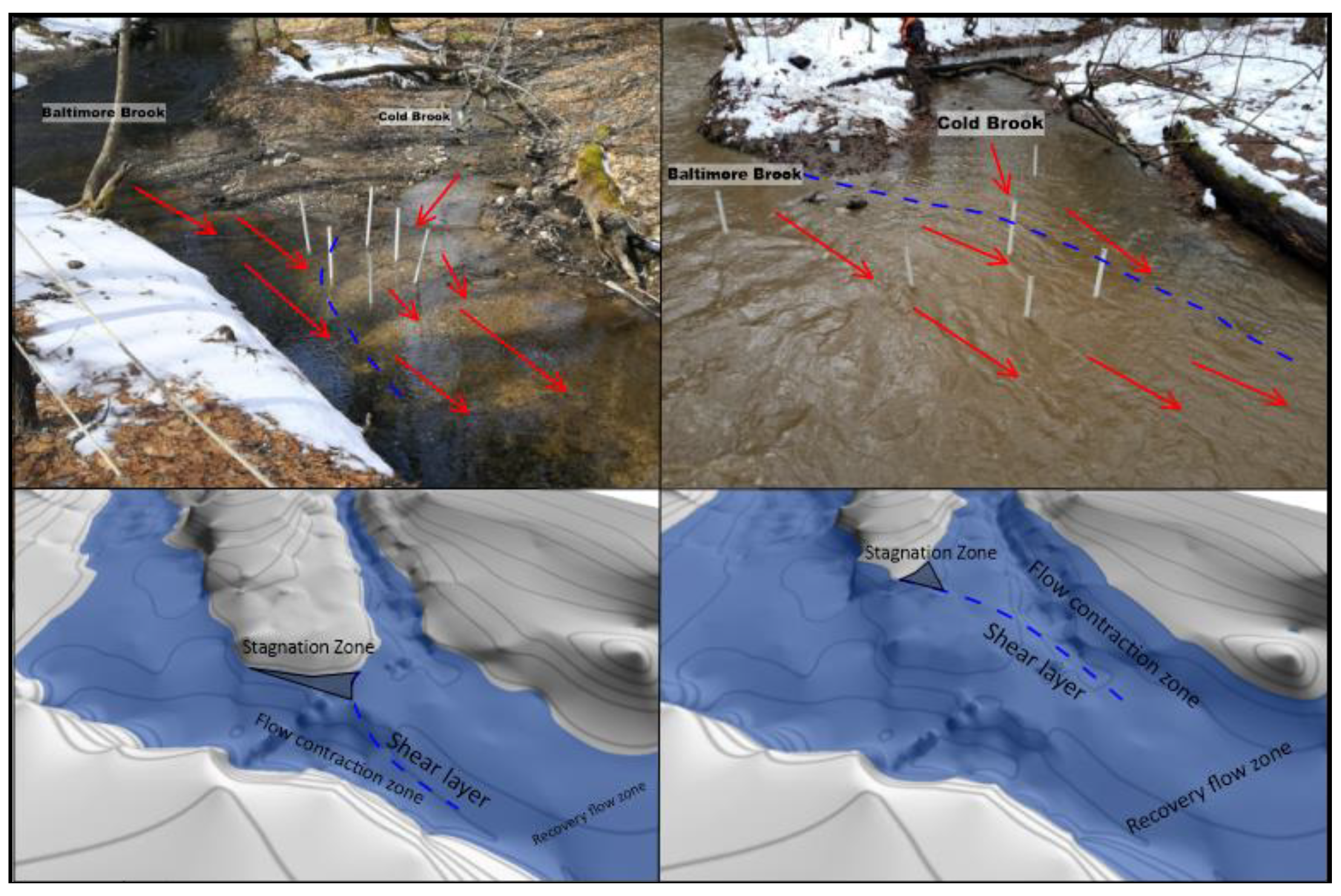
BB and CB were two first-order streams where water level was predominantly shallow over this field study, constituted by low-gradient velocities and pressure variations (Table 3). The planform geometry had a junction angle between the tributaries of approximately 80° in base-flow conditions, and a 40° angle during one high-flow event in December 2018 during liquid precipitation and snowmelt (Figure 5), while back-to-back angle between tributary and confluence downstream channel were: 145° and 150° (CB and BB) in base-flow conditions, whereas 142° and 162°, in high-flow conditions. Water levels, velocities, and flowrates at the BBCB confluence were measured only at the beginning of the study. However, these values could be considered as indicative of typical low flow conditions within an acceptable range of uncertainty because in those conditions USGS gauge downstream and in nearby rivers did not record any flow events greater than a 1.1-year frequency and indirect observations, including those from piezometer installations, showed no notable change in the water leveled. Larger velocities were observed from CB due to its bed morphology and steep riffle slope into the confluence, with a velocity ratio of BB to CB, VR = Ubb/Ucb = 0.42 and a momentum flux ratio, QR = ρQbbUbb/ρQcbUcb = 0.64. The location of the shear layer moved towards the right bank or BB side of the confluence due to the dominant CB flow velocity (see the dotted red line in Figure 5). Downward fluxes from prior channel forming flows eroded the BB riverbed forming a large scour hole within the CHZ (see Figure 6). Flow paths induced by bed topography in CB defined the length and width of a sand bar located downstream from the CHZ [12,40] and caused fine sand infiltration into the bed [24,45] which could cause lower Kv.
4.1.2. Bed Morphology
The confluence was characterized by low-gradient water surface slopes, with slightly higher slopes in the CB tributary in the 5 m upstream the junction. The area between BB and CB was abundant in outwash sediments and partially submerged during high-flow discharge event (i.e., in December after a sudden snow melt, Figure 5) complicating the localization of the BB and CB riverbanks (Figure 6). The deepest pool was found in BB, at a scour hole of approximately 40–50 cm wide, along the outer bank as common in pool-riffle rivers [41,42,43], while CB and the CHZ depths were mostly without pool and averaged 5–10 cm. Sediment scour was located in the BB pool and outer bank, and depositional areas were observed downstream the confluence on the left bank and CB flow side, with a high presence of pebbles and fine sand on the river bottom.
4.1.3. Hydraulic Conductivity and Grain Size Analysis
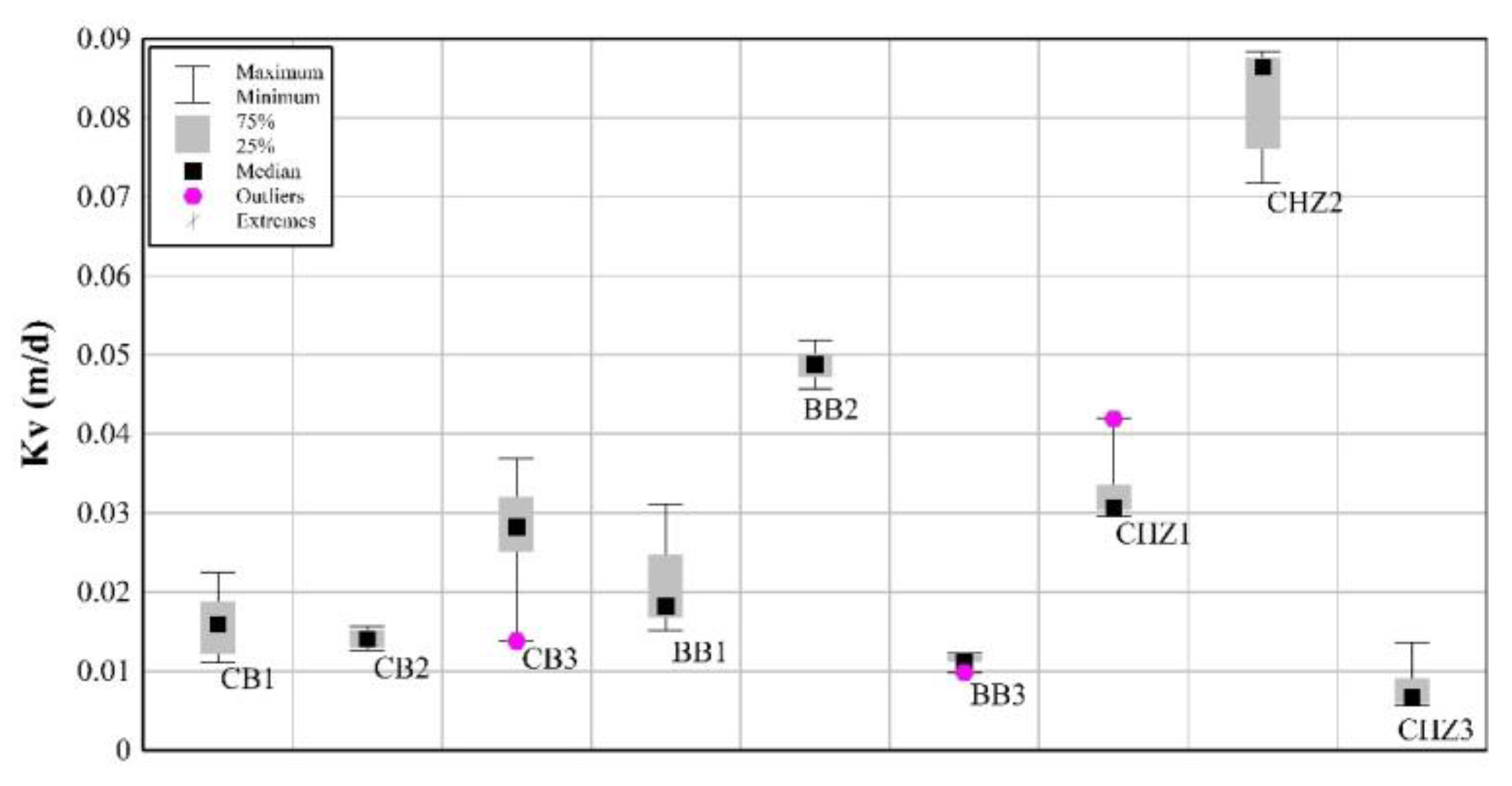
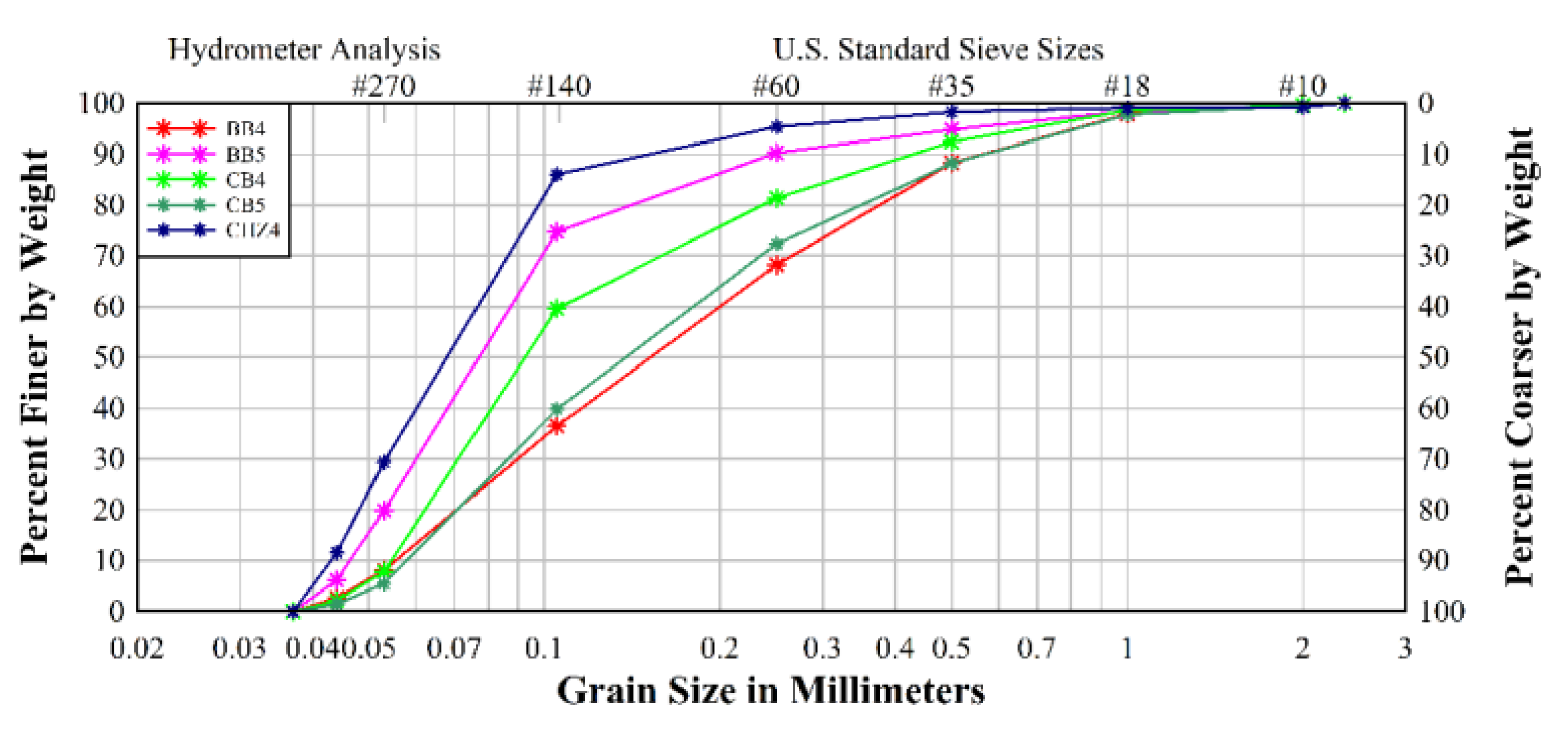
Hydraulic conductivity tests result showed very low Kv values throughout the confluence. The values ranged from 0.09 to 0.005 m/d (Figure 7). According to mean and median Kv in BB and CB and the CHZ, CHZ3 had the smallest hydraulic conductivity. That area was subjected to sand (0.075 mm < PZ < 2 mm) deposition during fall low flow season that might have decreased Kv values due to layering of streambed sediments [44]. In fact, laboratory analysis of substrate samples showed that grain size in the confluence bed was mostly composed of fine sand (0.063 mm < PZ < 0.2 mm). The average of cumulative percentages by weight is listed in Table 4. The silt-clay fraction, instead, was larger in CHZ sediment sample while, on average, BB and CB showed lower values (Figure 8).
4.2. Temperature Time Series and VFLUX Code Application
Temperature profiles obtained across the confluence were used in VFLUX to get directions (noted as positive values indicate downwelling flux), magnitudes and patterns of vertical hyporheic fluxes in multiple locations over several months. Temperature differences between the groundwater and surface water in FS-BBCB1 and FS-BBCB2 were less than 2 °C and 1 °C, respectively.
4.2.1. Fall Low Flow and Snow-Melt Season
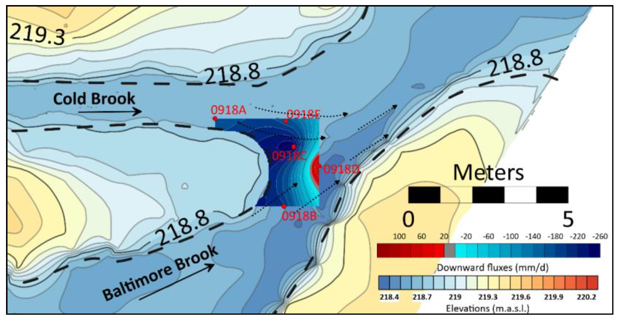
During the fall season, variations in flux direction within the confluence were observed within the top 20 cm of the riverbed by temperature profile analysis. The probes at greater depths did not register sufficient temperature variation to reveal as vertical hyporheic fluxes. The vertical hyporheic fluxes had seasonal trends. In late summer, from 16 to 23 September, fluxes ranged from +1.12 mm/day (downwelling) to −2.61 mm/day, with four of these upwelling fluxes in the majority of the confluence (0918A, 0918B, 0918C, and 0918E, Figure 9). The single downwelling flux (0918D) was observed at the scour hole section of the confluence.
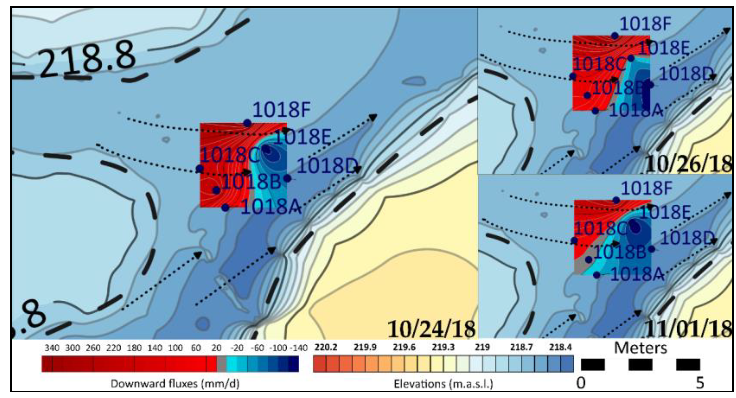
In the mid-fall period, from 23 October to 6 November, there were three distinct patterns of vertical hyporheic exchange, during which time the site received 55 mm of precipitation and river stage increased ~6 cm or 30%. At the beginning of this wet period, from 23 to 25 October, maximum downwelling fluxes of 405 mm/day were observed around rods 1018A, 1018B, 1018C, and 1018F in the upstream section, and upwelling in the downstream section (Figure 10). In this period, the maximum daily upwelling fluxes gradually transitioned from −400 to −145 mm/day at rod 1018E, while upwelling remained steady at 1018D. Second, on 26 October, rod 1018E flux direction changed to moderately downwelling from a strong upwelling, and the upwelling at 1018D in the BB section of the confluence increased to a maximum of −140 mm/day. The third pattern emerged from 1 to 6 November when the upwelling hyporheic flux shifted further upstream along the BB side of the confluence to rods 1018A and the downwelling at rod 1018B ceased and became neutral (Figure 10). These changes in flux pattern suggest that BB transitioned to greater upwelling during the wet period, while downwelling flux in the CB section of the confluence was relatively steady.
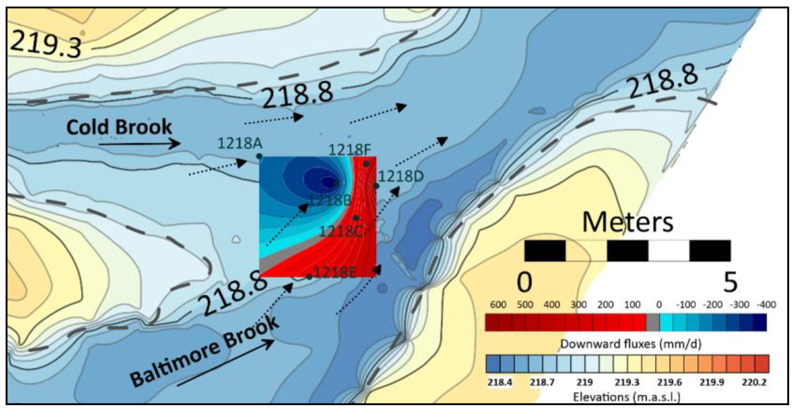
In late fall during 2–4 December, after a month of little rainfall, the hyporheic fluxes reversed from the mid-fall pattern. The upwelling fluxes were organized along the CB upstream section of the confluence, while downwelling fluxes were observed along the downstream confluence section and into the upper BB section. In this period, the CB temperature rods (1218A and 1218B) registered upwelling fluxes, while rods 1218D and 1218E had strong downwelling fluxes (Figure 11). The flux rates ranged from 602 mm/day to −397 mm/day, reaching greater values than in the mid-fall period. As with the late summer period, but unlike the mid-fall with the rains, the December fluxes were steady values over the sampling period even though there was a steady decline in river stage.
4.2.2. Spring High Flow Season
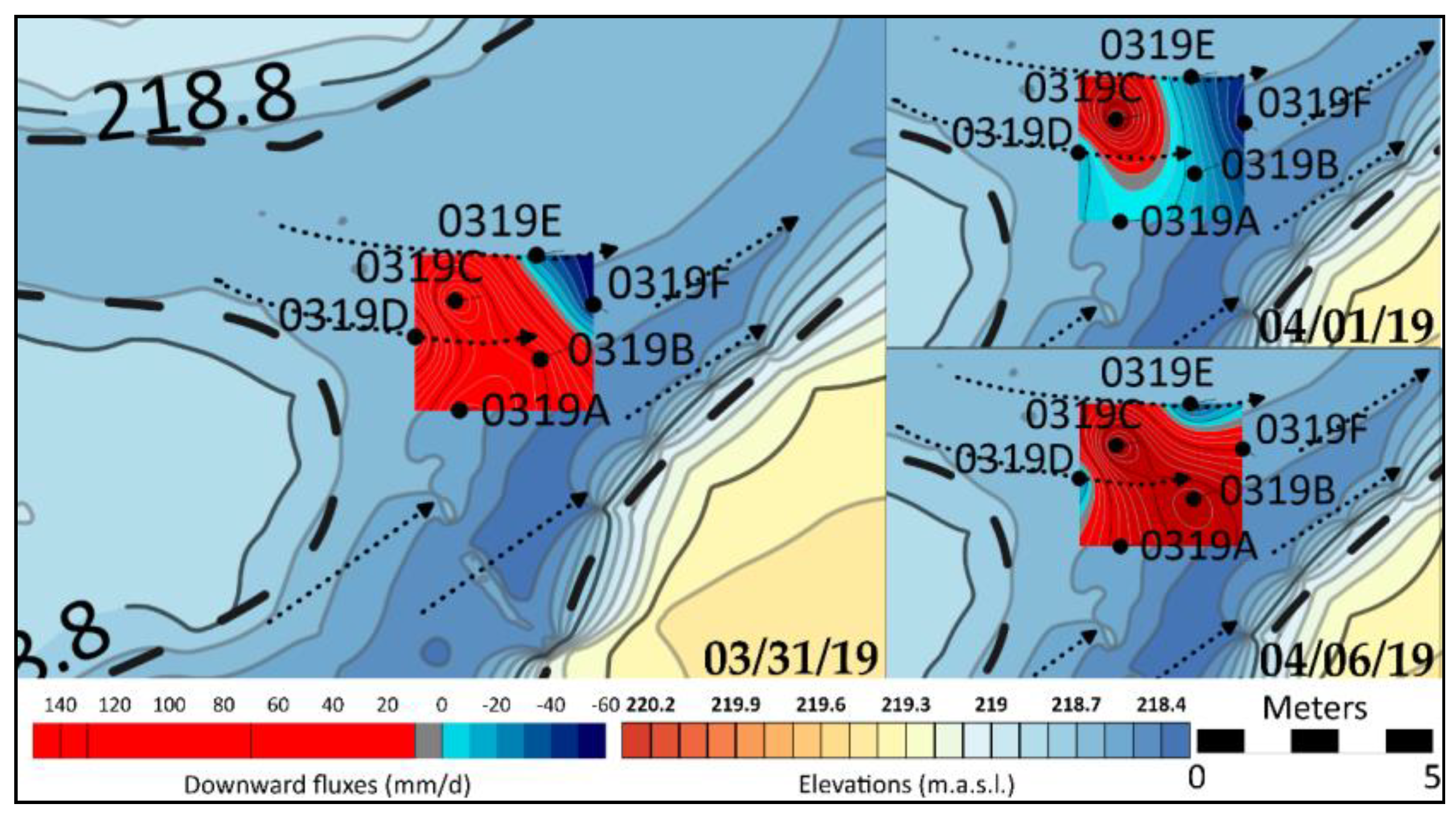
The spring season brought changes in river flow, and this was used to organize three periods of distinct patterns in hyporheic flux. The changes in flow were attributed to a rainfall event between 29 and 31 March and another period of rainfall between 3 and 7 April. At the end of the March rained, downwelling fluxes were observed downstream of the confluence, with an isolated corner of upwelling at rods 0319E and 0319F (Figure 12).
During the period between the rains, on 1 April, the hyporheic flux pattern shifted and upwelling now existed across most of the confluence, at all rods except for the rod 0319C in the upper confluence where CB entered. The continuation of rains from 3 to 7 April resulted in a general return to the late March pattern of flux, with downwelling extending across most of the monitoring section, and upwelling at rod 0319E in the downstream section along the CB region, as well as at rod 0319D near the confluence vertex.
4.3. Discussion
Regional to local drivers of hyporheic exchange can gather within the confluence hydrodynamic zone. At a regional scale, the dominant drivers of hyporheic exchange flux patterns are the relative levels of river stage and groundwater [11,12,13,21,22], while at local scale bed morphology, soil heterogeneity, and channel velocity influence hyporheic exchange [13]. In pool-riffle channels with moderate slope, such as BB and CB, hyporheic exchange is usually driven by the variability of the spatial distribution of channel velocity and resulting pressure head [40]. Downwelling and upwelling zones are usually located on riffle head with lower velocities (higher pressure) and riffle tail with higher velocities (lower pressure), respectively [25]. Local topography is a prominent driver of changes in hyporheic flux direction when bed depth increases or decreases in the downstream direction, and the concave or convex nature water surface profiles can also change hyporheic flux direction [45]. On bedforms, past studies demonstrated that close to the detachment point downstream of dune crest and to the reattachment point on the dune stoss side are minimum and maximum pressure regions, respectively, creating patterns of upwelling and downwelling [46].
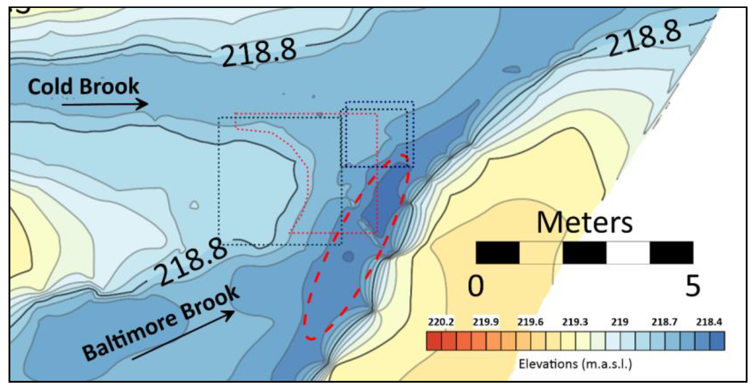
This field study found distinct upwelling or downwelling patterns of hyporheic exchange flux and observed its variation across eight months from late summer to spring seasons. During this period, these patterns exhibited variability while hydrodynamic and hydrological condition were changing. However, as BB and CB were ungauged streams, daily measurements of discharge, and water stage were not available. These data were collected at some characteristic locations of the confluence (Figure 13), such as the confluence junction (September 2018 and December 2018), the scour hole (September 2018) and the shear layer (October/November 2018 and March/April 2019), where the aforementioned patterns of hyporheic exchange observed in pool-riffle channels might be modified by the confluence hydrodynamic and morphodynamics features.
4.3.1. Effect of Scour Hole on the Hyporheic Fluxes
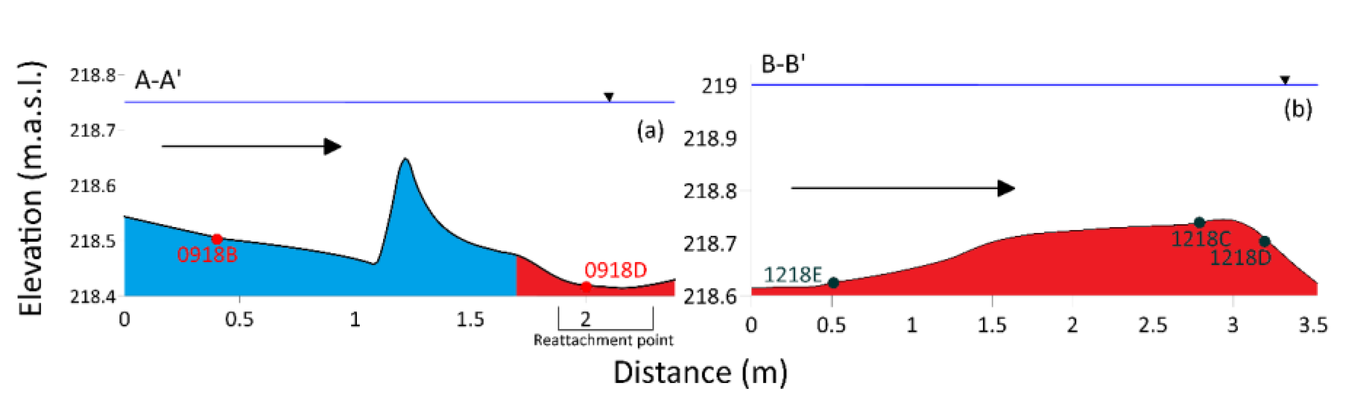
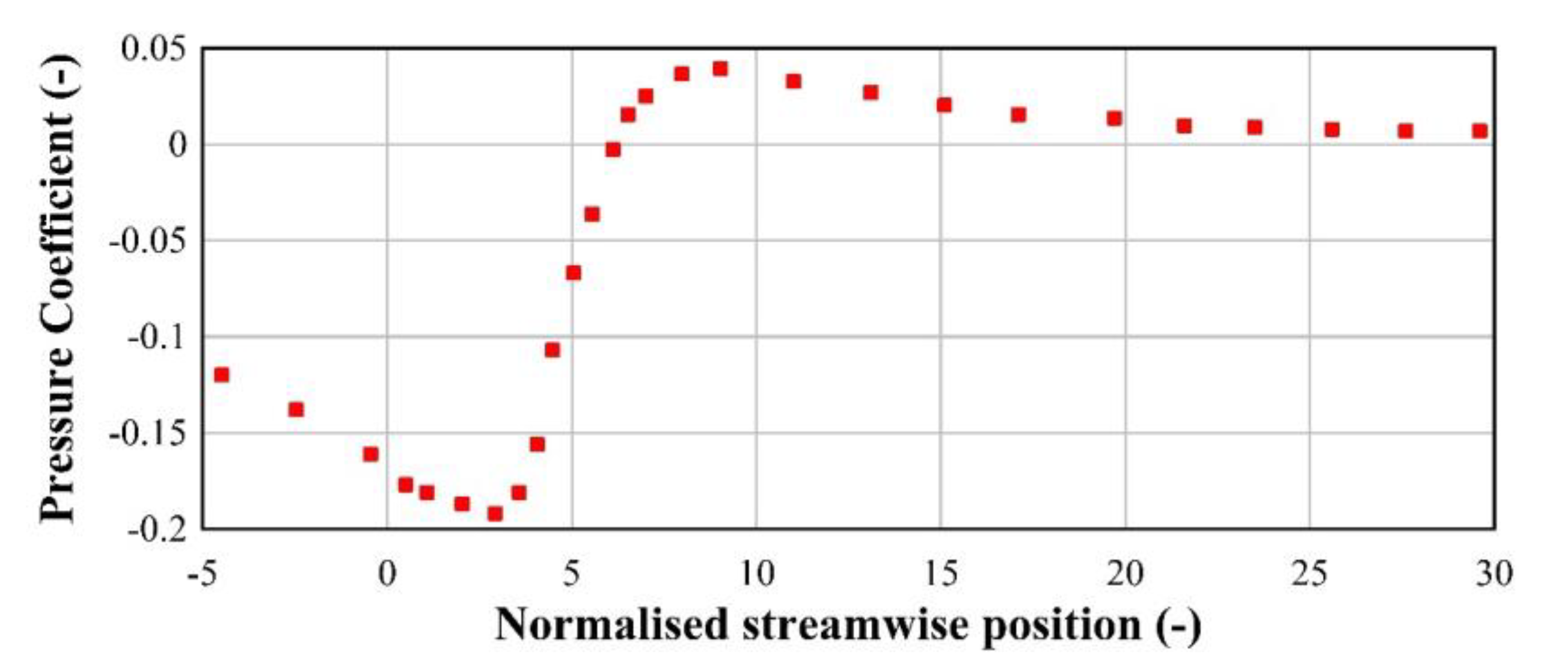
In September 2018, at the confluence entrance the flow from CB tended toward the BB bank (Figure 5 left). At that time the area of measurement was located just downstream the junction corner, where the flow from BB is featuring an abrupt step at the entrance of the scour hole (Figure 9, Figure 13, Figure 14, Figure 15a). The flow over a step is a classic type of separation flow, termed backward facing step flow (BFSF), which has been extensively investigated using both experimental [47] and numerical methods [48] in laminar and turbulent flows. It is well-known that in the BFSF downstream the step bottom pressure is going down which is followed by a rapid increase to get a maximum close to the reattachment point. While in laminar flow the location of the minimum/maximum pressure point is depending upon the step height-based Reynolds number [48], in a turbulent BFSF the point of minimum and maximum bed pressure is located at x/Hstep = 3.0 and x/Hstep = 9, respectively (Figure 16) [47]. In our case, as the step height is approximately 0.15 m, the maximum pressure should be located about 0918D point (Figure 15a). This is consistent with the observed hyporheic fluxes, which were directed upward (upwellings) upstream and immediately downstream of the step bordering the scour hole and downward (downwelling) around 0918D point, where flow reattachment and maximum pressure should be located. On the other hand, in the area of measurement, the flow from CB is moving over a plane bed, where flow was accelerating, and upwelling was observed.
It should be noted that the PVC rod piezometer installations across the CHZ indirectly showed no notable change in the bed morphology. Additionally, the location of the scour hole remained unchanged during the field study. It is expected that changes in the location of the scour hole occurring on a longer timescale could modify the hyporheic exchange at the confluence.
4.3.2. Effect on Variations in Confluence Geometry on the Hyporheic Fluxes
In December 2018 a snowmelt event increased discharge and water level at the confluence and the junction angle/location as well as the circulation at the confluence was accordingly modified (Figure 5 right). The confluence junction as well as the stagnation zone shifted upstream, while the location of the shear layer moved toward the CB bank (Figure 5 right). The area of measurement in December 2018 was partially overlapping with that of September 2018, as it was located more upstream and it was only bordering the scour hole (Figure 11, Figure 13, Figure 14 and Figure 15b). In December 2018, in that area, the flow partially moves over the location of the junction in low flow conditions (Figure 15b), where upwelling was observed, and partially over a stepped bed, where downwelling was measured. Comparatively, the area and the rate of downwelling increased from September to December 2018. This might be explained by the observed changes in the main flow patterns at the confluence entrance.
4.3.3. Effect of Secondary Flows on the Hyporheic Fluxes
In October/November 2018 and March/April 2019 the area of measurement was located downstream of that in September and December 2018, in the shear layer region (Figure 13), where hydrodynamics is generally characterized by complex 3D patterns and helical flow cells are also often observed [40], although their presence, characteristics and origin need further investigations [19,49]. Following the back-to-back bend or meander analogy, these cells are expected to converge at the surface in the center of the channel and to diverge near the bed [1,40,41]. Furthermore, these helical cells are associated with downward and upward flow patterns in the water column which could have an impact even on the hyporheic exchange. Cheng et al. [22] observed at the confluence between Juehe River and Haohe River (junction angle, 110°) downwelling patterns in the area across the shear layer where helicoidal flow cells were located. They argued that the encounter and impact of the two tributaries created in that area a downward flow causing a downwelling hyporheic exchange. In the present study, it was not possible to confirm or not the presence of helical cells at the BBCB confluence. However, confluence planform (Figure 6) and the related bend-like flow patterns of the tributaries might suggest the presence of the above secondary circulation. In October/November 2018, downwelling/upwelling was observed on the CB/BB side of the area of measurement, respectively, but some variations were noted from October to November (Figure 10). In March/April, the distribution of the hyporheic fluxes was different, as almost only downwelling was measured on 31 March and 6 April, while on 1 April upwelling was predominant (Figure 12). To try to explain this strong variability, two cross-sections located in the measurement area October/November 2018 and March/April 2019 were considered (Figure 14) and the distribution of the hyporheic fluxes was plotted (Figure 17a,b). In October/November 2018 and March/April 2019 a downwelling region was observed across the shear layer about the scour hole (Figure 17a,b). This finding is consistent with the observations by Cheng at al. [22] and it could be related to the bed pressure distribution across the back-to-back bend at the confluence. At the end, the observed patterns in the distribution of hyporheic fluxes seem to be related to the hydrodynamics and morphodynamics characteristics about the confluence and their changes during the hydrological cycle.
Given the role of confluence junction angle in influencing hyporheic exchange flux, patterns of hyporheic fluxes are expected to fluctuate with changes in flow depth if the junction angle changes with channel depth of water. Further, given the role of momentum flux ratio influencing hyporheic flux, differences in water characteristics that lead to changes in density, temperature, conductivity, and suspended sediment concentration would likely trigger changes in hyporheic exchange patterns [19].
5. Conclusions
In the literature about the environmental interfaces [50] few studies are available regarding the hyporheic exchange at river confluences. This experimental research characterized the spatial and temporal patterns of vertical hyporheic exchange flux about a small headwater confluence in the USA. The field data and its analysis were used to explain the observed patterns of hyporheic exchange by confluence hydrology, geometry, hydrodynamics, morphodynamics, grain size distribution, and vertical hydraulic conductivity. Furthermore, the effect on the hyporheic exchange due to some classical features of a confluence flow, such the stagnation zone, flow deflection, and contraction zone, including the scour hole, and the shear layer was investigated. Finally, to expand on the two prior studies of hyporheic exchange at a confluence under baseflow, this study monitored across eight months to capture low flow and high flow patterns. Principal outcomes found within this research are:
- Soil samples showed that BBCB site was mostly sandy-gravel and hydraulic conductivity tests reported very low values, suggesting that local sediment transport processes allocated fine sediments into pores, reducing soil permeability.
- Confluence geometry, hydrodynamics, and morphodynamics were found to significantly affect hyporheic exchange rate and patterns. In September and December 2018, local scale bed morphology, such as the confluence scour hole and minor topographic irregularities, influenced the distribution of bed pressure head and the related patterns of downwelling/upwelling.
- Variation in hydrological conditions during a high flow event in December 2018 survey were seen to modify confluence geometry, such as junction angle and position, and, in turn, flow circulation patterns, shifting back the stagnation zone and relocating the shear layer. The hyporheic flux pattern in low flow conditions was modified where upwelling was mostly observed, and partially over a stepped bed, downwelling was measured.
- In October/November 2018 and March/April 2019, classical back-to-back bend planform and the related secondary circulation might probably affect hyporheic exchange patterns around the confluence shear layer as already documented in the literature [22].
- Seasonal hydrological condition should be taken into account. There was a visible pattern among October 2018 and March 2019 temperature rods: in these two cases fluxes were not only driven by morphological or hydrodynamic conditions.
Follow-up work must focus on the relationship among soil permeability, flow momentum changes, and groundwater which are still under investigation for this complex study. A continuous monitoring of streams discharge, velocity, and water depth, as well as and vertical fluxes is advisable to reduce the uncertainty in the analysis of hyporheic dynamics within a complex riverine system such as a confluence and to highlight main factors such as seasonal and regional changes and drivers of surface-subsurface water interaction.
Author Contributions
All the authors equally participated to this study. I.M. and T.E. conducted the field surveys while C.G. participated to the post-processing analysis. I.M., C.G. and T.E. wrote the manuscript. All authors have read and agreed to the published version of the manuscript.
Funding
This research received no external funding.
Acknowledgments
The research was carried out during the PhD Project in “Civil System Engineering” of the first Author. He also shows his gratitude to SUNY for hosting, support and instrumentation and thanks Guy Swenson for assistance with all field campaigns. Collaboration with staff of the Environmental Resources Engineering Department of the SUNY-ESF is gratefully acknowledged. The second author acknowledges the financial support from the Exchange Program for Professors and Researchers of the University of Napoli Federico II for the year 2018.
Conflicts of Interest
The authors declare no conflict of interest.
References
- Mosley, M.P. An experimental study of channel confluences. J. Geol. 1976, 83, 535–562. [Google Scholar] [CrossRef]
- Best, J.L. Sediment transport and bed morphology at river channel confluences. Sedimentology 1988, 35, 481–498. [Google Scholar] [CrossRef]
- Best, J.L.; Rhoads, B.L. Sediment Transport, Bed Morphology and The Sedimentology of River Channel Confluences. In River Confluences, Tributaries and the Fluvial Network; Rice, S., Roy, A., Rhoads, B.J., Eds.; John Wiley & Sons: Hoboken, NJ, USA, 2008; pp. 45–72. [Google Scholar]
- Gualtieri, C.; Filizola, N.; Oliveira, M.; Santos, A.M.; Ianniruberto, M. A field study of the confluence between Negro and Solimões Rivers. Part 1: Hydrodynamics and sediment transport. Compt. Rend. Geosci. 2018, 350, 31–42. [Google Scholar] [CrossRef]
- Ianniruberto, M.; Trevethan, M.; Pinheiro, A.; Andrade, J.F.; Dantas, E.; Filizola, N.; Santos, A.; Gualtieri, C. A field study of the confluence between Negro and Solimões Rivers. Part 2: Riverbed morphology and stratigraphy. Compt. Rend. Geosci. 2018, 350, 43–54. [Google Scholar] [CrossRef]
- Errico, A.; Lama, G.F.C.; Francalanci, S.; Chirico, G.B.; Solari, L.; Preti, F. Flow dynamics and turbulence patterns in a drainage channel colonized by common reed (Phragmites australis) under different scenarios of vegetation management. Ecol. Eng. 2019, 133, 39–52. [Google Scholar] [CrossRef]
- Fernandes, C.; Podos, C.J.; Lundberg, J.G. Amazonian ecology: Tributaries enhance the diversity of electric fishes. Science 2004, 305, 1960–1962. [Google Scholar] [CrossRef] [Green Version]
- Grant, E.H.C.; Lowe, W.H.; Fagan, W.F. Living in the branches: Population dynamics and ecological processes in dendritic networks. Ecol. Lett. 2007, 10, 165–175. [Google Scholar] [CrossRef]
- Gualtieri, C.; Ianniruberto, M.; Filizola, N.; Santos, R.; Endreny, T. Hydraulic complexity at a large river confluence in the Amazon basin. Ecohydrology 2017, 10, e1863. [Google Scholar] [CrossRef]
- Gualtieri, C.; Abdi, R.; Ianniruberto, M.; Filizola, N.; Endreny, T. A 3D analysis of spatial habitat metrics about the confluence of Negro and Solimões rivers, Brazil. EcoHydrology 2020, 13, e2166. [Google Scholar] [CrossRef]
- Boano, F.; Harvey, J.W.; Marion, A.; Packman, A.I.; Revelli, R.; Ridolfi, L.; Wörman, A. Hyporheic flow and transport processes: Mechanisms, models, and biogeochemical implications. Rev. Geophys. 2014, 52, 603–679. [Google Scholar] [CrossRef]
- Cardenas, B.M.; Wilson, J.L.; Zlotnik, V.A. Impact of heterogeneity, bed forms, and stream curvature on subchannel hyporheic exchange. Water Resour. Res. 2004, 40. [Google Scholar] [CrossRef] [Green Version]
- Tonina, D. Surface water and streambed sediment interaction: The hyporheic exchange. In Fluid Mechanics of Environmental Interface, 2nd ed.; Gualtieri, C., Mihailović, D.T., Eds.; Taylor & Francis Ltd.: London, UK, 2012; pp. 255–294. [Google Scholar]
- Harvey, J.W.; Bencala, K.E. The Effect of Streambed Topography on Surface-Subsurface Water Exchange in Mountain Catchments. Water Resour. Res. 1993, 29, 89–98. [Google Scholar] [CrossRef]
- Stonedahl, S.H.; Harvey, J.W.; Wörman, A.; Salehin, M.; Packman, A.I. A multiscale model for integrating hyporheic exchange from ripples to meanders. Water Resour. Res. 2010, 46. [Google Scholar] [CrossRef] [Green Version]
- Revelli, R.; Boano, F.; Camporeale, C.; Ridolfi, L. Intra-meander hyporheic flow in alluvial rivers. Water Resour. Res. 2008, 44. [Google Scholar] [CrossRef]
- Endreny, T.A.; Lautz, L.; Siegel, D.I. Hyporheic flow path response to hydraulic jumps at river steps: Flume and hydrodynamic models. Water Resour. Res. 2011, 47. [Google Scholar] [CrossRef]
- Constantinescu, G.; Miyawaki, S.; Rhoads, B.; Sukhodolov, A.; Kirkil, G. Structure of turbulent flow at a river confluence with a momentum and velocity ratios close to 1: Insight from an eddy-resolving numerical simulation. Water Resour. Res. 2011, 47. [Google Scholar] [CrossRef]
- Gualtieri, C.; Ianniruberto, M.; Filizola, N. On the mixing of rivers with a difference in density: The case of the Negro/Solimões confluence, Brazil. J. Hydrol. 2019, 578. [Google Scholar] [CrossRef]
- Yuan, S.; Tang, H.; Xiao, Y.; Qiu, X.; Xia, Y. Water flow and sediment transport at open-channel confluences: An experimental study. J. Hydraul. Res. 2017, 56, 333–350. [Google Scholar] [CrossRef]
- Song, J.; Zhang, G.; Wang, W.; Liu, Q.; Jiang, W.; Guo, W.; Tang, B.; Bai, H.; Dou, X. Variability in the vertical hyporheic water exchange affected by hydraulic conductivity and river morphology at a natural confluent meander bend. Hydrol. Process. 2017, 31, 3407–3420. [Google Scholar] [CrossRef]
- Cheng, D.; Song, J.; Wang, W.; Zhang, G. Influences of riverbed morphology on patterns and magnitudes of hyporheic water exchange within a natural river confluence. J. Hydrol. 2019, 574, 75–84. [Google Scholar] [CrossRef]
- Zarriello, P.J. A Precipitation-Runoff Model for part of the Ninemile Creek Watershed near Camillus, Onondaga County, New York, USA; Geological Survey Water-Resources Investigation Reports: Reston, VA, USA, 1999. [Google Scholar]
- Anibas, C.; Fleckenstein, J.H.; Volze, N.; Buis, K.; Verhoeven, R.; Meire, P.; Batelaan, O. Transient or steady-state? Using vertical temperature profiles to quantify groundwater-surface water exchange. Hydrol. Process. 2009, 23, 2165–2177. [Google Scholar] [CrossRef]
- Gariglio, F.P.; Tonina, D.; Luce, C.H. Spatiotemporal variability of hyporheic exchange through a pool-riffle-pool sequence. Water Resour. Res. 2013, 49, 7185–7204. [Google Scholar] [CrossRef]
- Rau, G.C.; Andersen, M.S.; McCallum, A.M.; Acworth, R.I. Analytical methods that use natural heat as a tracer to quantify surface water-groundwater exchange, evaluated using field temperature records. Hydrogeol. J. 2010, 18, 1093–1110. [Google Scholar] [CrossRef]
- Zarnetske, J.P.; Gooseff, M.N.; Breck Bowden, W.; Greenwald, M.J.; Brosten, T.R.; Bradford, J.H.; McNamara, J.P. Influence of morphology and permafrost dynamics on hyporheic exchange in arctic headwater streams under warming climate conditions. Geophys. Res. 2008, 35. [Google Scholar] [CrossRef] [Green Version]
- Lee, D.R.; Cherry, J.A. A field exercise on groundwater flow using seepage meters and mini-piezometers. J. Geol. Educ. 1978, 27, 6–10. [Google Scholar] [CrossRef]
- Kennedy, C.D.; Genereux, D.P.; Corbett, D.R.; Mitasova, H. Design of a light-oil piezomanometer for measurement of hydraulic head differences and collection of groundwater samples. Water Resour. Res. 2007, 43. [Google Scholar] [CrossRef]
- Hvorslev, M.J. Time Lag and Soil Permeability in Groundwater Observations; Tech. rep.; Waterways Experiment Station, Corps of Engineers, U.S. Army: Vicksburg, MS, USA, 1951. [Google Scholar]
- Chen, X. Measurement of streambed hydraulic conductivity and its anisotropy. Environ. Geol. 2000, 39. [Google Scholar] [CrossRef]
- Vuković, M.; Soro, A. Determination of Hydraulic Conductivity of Porous Media from Grain-Size Composition, 1st ed.; Water Resources Publications: Littleton, CO, USA, 1992. [Google Scholar]
- Lautz, K.L.; Kranes, N.T.; Siegel, D.I. Heat tracing of heterogeneous hyporheic exchange adjacent to in-stream geomorphic features. Hydrol. Process. 2010, 24, 3074–3086. [Google Scholar] [CrossRef]
- Gordon, R.P.; Lautz, L.K.; Briggs, M.A.; McKenzie, J.M. Automated calculation of vertical pore-water flux from field temperature time series using the VFLUX method and computer program. J. Hydrol. 2011, 141, 142–158. [Google Scholar] [CrossRef]
- Irvine, D.J.; Lautz, L.K.; Briggs, M.A.; Gordon, R.P.; McKenzie, J.M. Experimental evaluation of the applicability of phase, amplitude, and combined methods to determine water flux and thermal diffusivity from temperature time series using VFLUX 2. J. Hydrol. 2015, 531, 728–737. [Google Scholar] [CrossRef] [Green Version]
- Young, P.C.; Taylor, C.J.; Tych, W.; Pegregal, D.J.; Mckenna, P.G. The Captain Toolbox; Centre for Research on Environmental Systems and Statistics, Lancaster University: Lancaster, UK, 2010. [Google Scholar]
- Keery, J.; Binley, A.; Crook, N.; Smith, J.W.N. Temporal and spatial variability of groundwater-surface water fluxes: Development and application of an analytical method using temperature time series. J. Hydrol. 2007, 336, 1–16. [Google Scholar] [CrossRef]
- Hatch, C.E.; Fisher, A.T.; Revenaugh, J.S.; Constantz, J.; Ruehl, C. Quantifying surface water-groundwater interactions using time series analysis of streambed thermal records: Method development. Water Resour. Res. 2006, 42. [Google Scholar] [CrossRef] [Green Version]
- Stallman, R.W. 1965. Steady one-dimensional fluid flow in a semi-infinite porous medium with sinusoidal surface temperature. J. Geophys. 1965, 70, 2821–2827. [Google Scholar] [CrossRef]
- Buffington, J.M.; Tonina, D. Hyporheic Exchange in Mountain Rivers II: Effects of Channel Morphology on Mechanics, Scales, and Rates of Exchange. Geogr. Compass 2009, 3, 1038–1062. [Google Scholar] [CrossRef]
- Rhoads, B.L.; Kenworthy, S.T. Flow structure at an asymmetrical stream confluence. Geomorphology 1995, 11, 273–293. [Google Scholar] [CrossRef]
- Rhoads, B.L.; Sukhodolov, A.N. Field investigation of three-dimensional flow structure at stream confluences: 1. Thermal mixing and time-averaged velocities. Water Resour. Res. 2001, 37, 2393–2410. [Google Scholar] [CrossRef]
- Rhoads, B.L.; Sukhodolov, A.N. Spatial and temporal structure of shear layer turbulence at a stream confluence. Water Resour. Res. 2004, 40. [Google Scholar] [CrossRef]
- Jiang, W.; Song, J.; Zhang, J.; Wang, Y.; Zhang, N.; Zhang, X.; Long, Y.; Li, J.; Yang, X. Spatial variability of streambed vertical hydraulic conductivity and its relation to distinctive stream morphologies in the Beiluo River, Shaanxi Province, China. Hydrogeol. J. 2015, 23, 1617–1626. [Google Scholar] [CrossRef]
- Anderson, J.K.; Wondzell, S.M.; Gooseff, M.N.; Haggerty, R. Patterns in stream longitudinal profiles and implications for hyporheic exchange flow at the H.J. Andrews Experimental Forest, Oregon, USA. Hydrol. Process. 2005, 19, 2931–2949. [Google Scholar] [CrossRef]
- Cardenas Bayany, M.; Wilson, J.L. Dunes, turbulent eddies, and interfacial exchange with permeable sediments. Water Resour. Res. 2007, 43, W08412. [Google Scholar] [CrossRef]
- Driver, D.M.; Seegmiller, H.L. Features of reattaching turbulent shear layer in divergent channel flow. AIAA J. 1985, 23, 163–171. [Google Scholar] [CrossRef]
- Gualtieri, C. Numerical simulations of laminar backward-facing step flow with FemLab 3.1. In Proceedings of the ASME Fluids Engineering Summer Conference (FEDSM2005), Houston, TX, USA, 19–23 June 2005. [Google Scholar]
- Szupiany, R.N.; Amsler, M.L.; Parsons, D.R.; Best, J.L. Morphology, flow structure, and suspended bed sediment transport at two large braid-bar confluences. Water Resour. Res. 2009, 45. [Google Scholar] [CrossRef] [Green Version]
- Cushman-Roisin, B.; Gualtieri, C.; Mihailović, D.T. Environmental Fluid Mechanics: Current issues and future outlook. In Fluid Mechanics of Environmental Interfaces, 2nd ed.; Gualtieri, C., Mihailović, D.T., Eds.; Taylor & Francis Ltd.: London, UK, 2012; pp. 3–17. [Google Scholar]
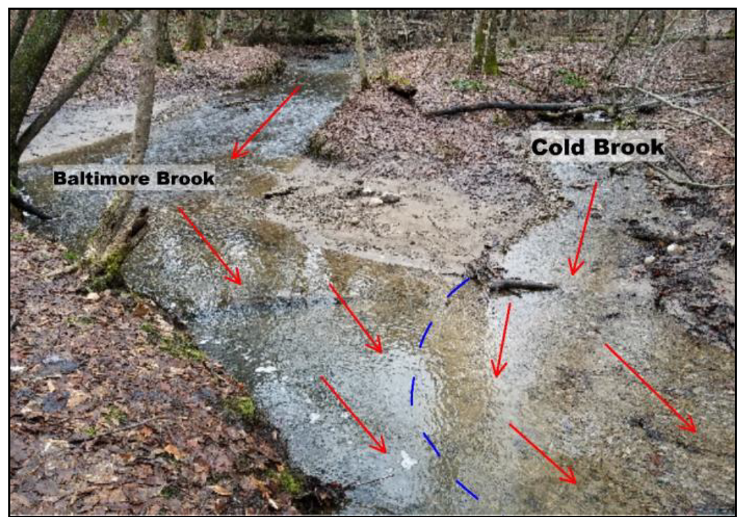
Figure 1.
BBCB confluence study site with red arrows showing flow direction and blue dashed line showing the location of the shear layer (picture taken on 1 January 2019).
Figure 1.
BBCB confluence study site with red arrows showing flow direction and blue dashed line showing the location of the shear layer (picture taken on 1 January 2019).

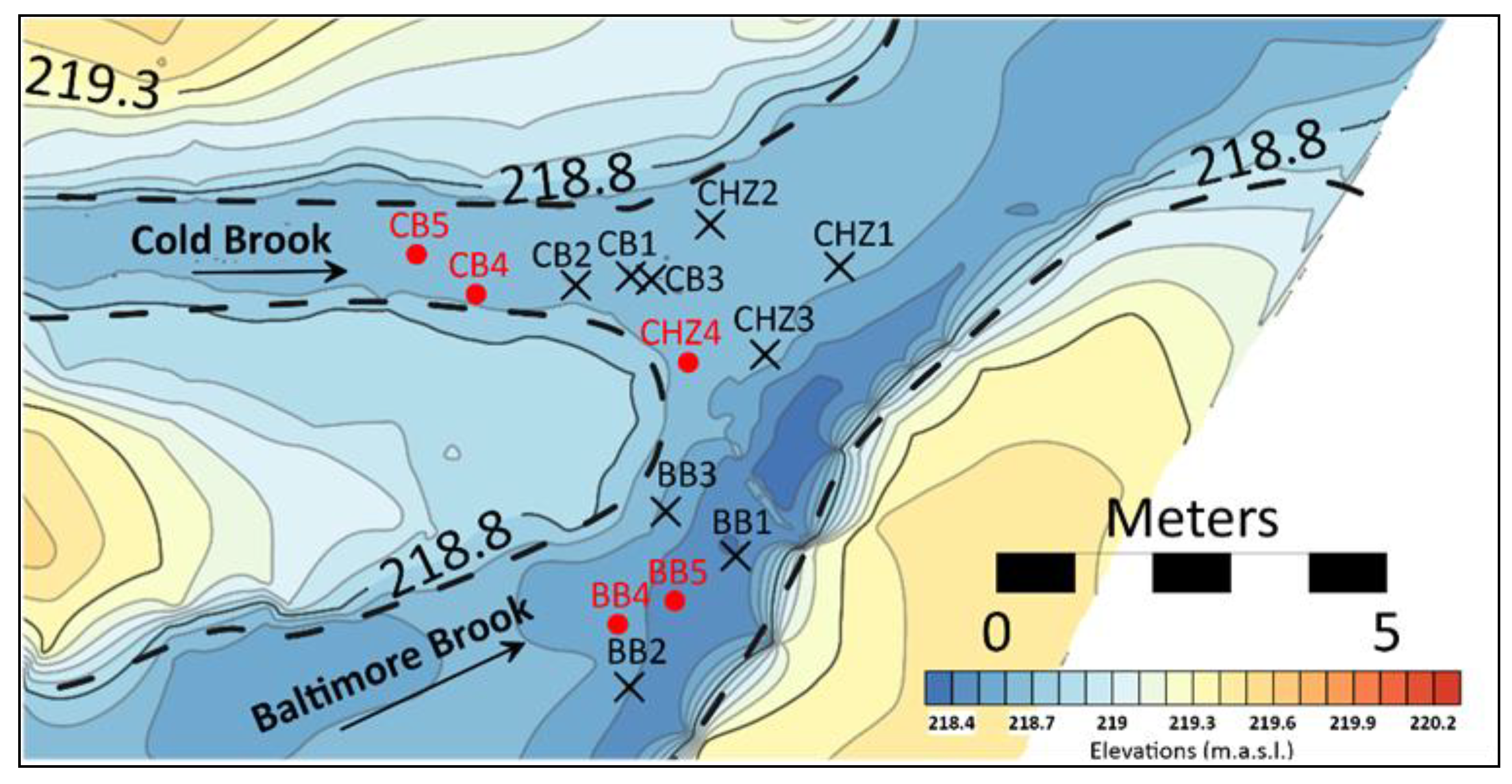
Figure 2.
Riverbed monitoring for FS-BBCB2 showing hydraulic conductivity test location (black X), soil sample test locations (red circle).
Figure 2.
Riverbed monitoring for FS-BBCB2 showing hydraulic conductivity test location (black X), soil sample test locations (red circle).

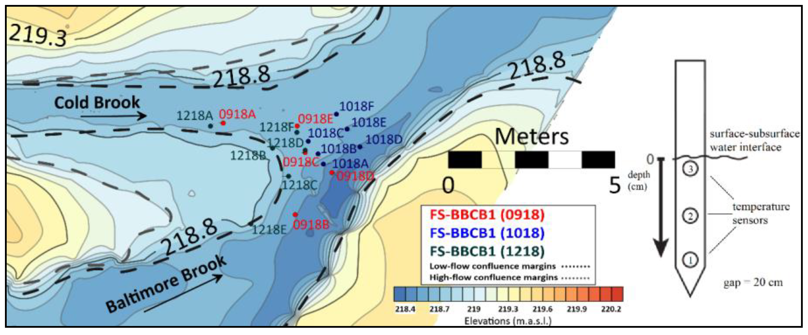
Figure 3.
Locations of temperature rods used for vertical hydraulic gradient tests, for FS-BBCB1 and the temperature rod setup (right).
Figure 3.
Locations of temperature rods used for vertical hydraulic gradient tests, for FS-BBCB1 and the temperature rod setup (right).

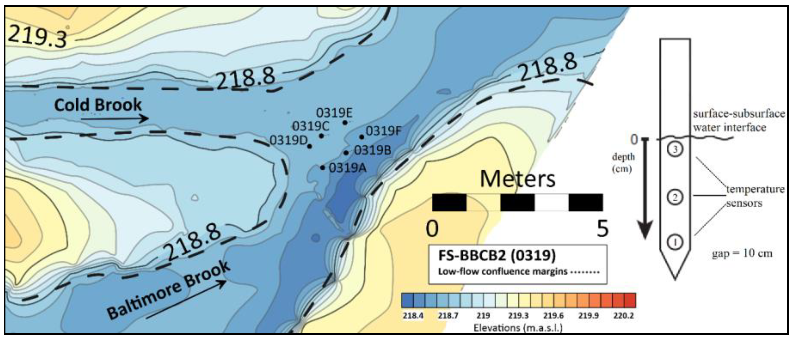
Figure 4.
Locations of temperature rods used for vertical hydraulic gradient tests, for FS-BBCB2 and the temperature rod setup (right).
Figure 4.
Locations of temperature rods used for vertical hydraulic gradient tests, for FS-BBCB2 and the temperature rod setup (right).

Figure 5.
Pictures of the confluence flow during low-flow (top left, 17 March 2019) and high-flow (top right, 2 December 2018) conditions, and 3D maps with the hydrodynamic features at a confluence (bottom).
Figure 5.
Pictures of the confluence flow during low-flow (top left, 17 March 2019) and high-flow (top right, 2 December 2018) conditions, and 3D maps with the hydrodynamic features at a confluence (bottom).

Figure 6.
Topography of watershed and riverbeds about the confluence zone, with black solid contour lines showing elevation above sea level (m). Black dotted lines delineate the active channel during low flow, and the red dotted ellipse delineates a scour hole.
Figure 6.
Topography of watershed and riverbeds about the confluence zone, with black solid contour lines showing elevation above sea level (m). Black dotted lines delineate the active channel during low flow, and the red dotted ellipse delineates a scour hole.

Figure 7.
Hydraulic conductivity values, Kv, (m/day) in box-and-whisker graph (bottom).

Figure 8.
Soil grain size distribution within the confluence, showing a fining of sand from upstream (BB and CB sites) to downstream into the confluence zone (CHZ).
Figure 8.
Soil grain size distribution within the confluence, showing a fining of sand from upstream (BB and CB sites) to downstream into the confluence zone (CHZ).

Figure 9.
Vertical hyporheic fluxes (mm/day) for September 2018, derived from temperature profiles. Downwelling and upwelling fluxes are represented by red and blue contours, respectively. The light blue contour represents an interpolated transitional zone.
Figure 9.
Vertical hyporheic fluxes (mm/day) for September 2018, derived from temperature profiles. Downwelling and upwelling fluxes are represented by red and blue contours, respectively. The light blue contour represents an interpolated transitional zone.

Figure 10.
Vertical hyporheic fluxes (mm/day) for 23 October to 6 November 2018, derived from temperature profiles. The light blue contour represents an interpolated transitional zone.
Figure 10.
Vertical hyporheic fluxes (mm/day) for 23 October to 6 November 2018, derived from temperature profiles. The light blue contour represents an interpolated transitional zone.

Figure 11.
Vertical hyporheic fluxes (mm/day) for December 2018, derived from temperature profiles. Grey contour represents an interpolated transitional zone. Confluence margins (grey dotted lines) refer to relatively high-flow condition.
Figure 11.
Vertical hyporheic fluxes (mm/day) for December 2018, derived from temperature profiles. Grey contour represents an interpolated transitional zone. Confluence margins (grey dotted lines) refer to relatively high-flow condition.

Figure 12.
Vertical hyporheic fluxes from FS-BBCB2 (0319). Upper left figure shows HEF pattern on 31 March, upper right figure on 1 April and lower figure on 6 April. Downwelling and upwelling fluxes are represented by red and blue contours, respectively.
Figure 12.
Vertical hyporheic fluxes from FS-BBCB2 (0319). Upper left figure shows HEF pattern on 31 March, upper right figure on 1 April and lower figure on 6 April. Downwelling and upwelling fluxes are represented by red and blue contours, respectively.

Figure 13.
VHF map extents from FS-BBCB1 and FS-BBCB2. The red polygon refers to the September 2018 map; dark green, dark blue, and black recall December 2018, October 2018, and March 2019 maps, respectively. The scour hole is individuated by the red ellipse.
Figure 13.
VHF map extents from FS-BBCB1 and FS-BBCB2. The red polygon refers to the September 2018 map; dark green, dark blue, and black recall December 2018, October 2018, and March 2019 maps, respectively. The scour hole is individuated by the red ellipse.

Figure 14.
Test points and cross-sections in FS-BBCB1 and FS-BBCB2. Red, light blue, dark blue, and black points refer to September 2018, December 2018, October 2018, and March 2019, respectively.
Figure 14.
Test points and cross-sections in FS-BBCB1 and FS-BBCB2. Red, light blue, dark blue, and black points refer to September 2018, December 2018, October 2018, and March 2019, respectively.

Figure 15.
Longitudinal sections (a) A–A’ and (b) B–B’ from Figure 14, with red fill depicting downwelling and blue fill depicting upwelling.
Figure 15.
Longitudinal sections (a) A–A’ and (b) B–B’ from Figure 14, with red fill depicting downwelling and blue fill depicting upwelling.

Figure 16.
Longitudinal distribution of pressure coefficient at the bottom in a turbulent backward facing step flow [47]. The dimensionless abscissa x/Hstep = 0 indicates the location of the step.
Figure 16.
Longitudinal distribution of pressure coefficient at the bottom in a turbulent backward facing step flow [47]. The dimensionless abscissa x/Hstep = 0 indicates the location of the step.

Figure 17.
Longitudinal sections (a) C–C’ and (b) D–D’ from Figure 14, with red fill depicting downwelling, and arrows showing secondary flow in the channel.
Figure 17.
Longitudinal sections (a) C–C’ and (b) D–D’ from Figure 14, with red fill depicting downwelling, and arrows showing secondary flow in the channel.


Table 1.
Summary of field campaigns carried out at Baltimore Woods Nature Center.
| Campaign | Bathymetry | Granulometry | Kv | Temperature Time Series | Date |
|---|---|---|---|---|---|
| FS-BBCB1 | X | X | X | September–December 2018 | |
| FS-BBCB2 | X | X | March–April 2019 |
Table 2.
Input parameters of VFLUX2 code. β is dispersivity, Kcal thermal conductivity, CsCal and CwCal volumetric heat capacity of sediment and water, respectively.
Table 2.
Input parameters of VFLUX2 code. β is dispersivity, Kcal thermal conductivity, CsCal and CwCal volumetric heat capacity of sediment and water, respectively.
| Parameter | Value | Unit |
|---|---|---|
| β | 0.001 | m |
| Kcal | 0.0045 | cal/(s·cm·°C) |
| CsCal | 0.5 | cal/(cm3·°C) |
| CwCal | 1.0 | cal/(cm3·°C) |
Table 3.
Low flow active channel width, depth, average velocity, discharge, Froude and Reynolds numbers in BB, CB, and in the CHZ. Data for BB and CB were collected 1.5 m upstream of the junction, and data for CHZ were collected 3 m downstream of the river junction.
Table 3.
Low flow active channel width, depth, average velocity, discharge, Froude and Reynolds numbers in BB, CB, and in the CHZ. Data for BB and CB were collected 1.5 m upstream of the junction, and data for CHZ were collected 3 m downstream of the river junction.
| Parameters | BB | CB | CHZ |
|---|---|---|---|
| Widthavg (m) | 2.20 | 1.00 | 3.09 |
| Depthavg (m) | 0.31 | 0.08 | 0.24 |
| Uavg (m/s) | 0.268 | 0.635 | 0.376 |
| Fr (-) | 0.155 | 0.735 | 0.248 |
| Re (-) | 81720 | 48387 | 88411 |
| Qavg (m3/s) | 0.179 | 0.048 | 0.273 |
Table 4.
Sediment size distribution about the confluence, reporting the cumulative weight (%) for the two size fractions of sand and finer than sand, the particle diameter (mm) for 14%, 50%, and 84% finer than the diameter, coefficient of uniformity, and porosity.
Table 4.
Sediment size distribution about the confluence, reporting the cumulative weight (%) for the two size fractions of sand and finer than sand, the particle diameter (mm) for 14%, 50%, and 84% finer than the diameter, coefficient of uniformity, and porosity.
| Sample | BB4 | BB5 | CB4 | CB5 | CHZ4 |
|---|---|---|---|---|---|
| Cumulative weight (%) | |||||
| <0.053 mm | 2.67 | 6.21 | 2.13 | 1.44 | 11.56 |
| <2 mm | 99.64 | 99.46 | 99.57 | 99.52 | 99.18 |
| D14 (mm) | 0.064 | 0.032 | 0.059 | 0.065 | 0.080 |
| D50 (mm) | 0.152 | 0.077 | 0.092 | 0.136 | 0.068 |
| D84 (mm) | 0.435 | 0.180 | 0.304 | 0.416 | 0.103 |
| Coefficient of uniformity (η) | 2.607 | 2.368 | 2.270 | 2.530 | 1.135 |
| Porosity (n) | 0.406 | 0.404 | 0.415 | 0.408 | 0.439 |
© 2020 by the authors. Licensee MDPI, Basel, Switzerland. This article is an open access article distributed under the terms and conditions of the Creative Commons Attribution (CC BY) license (http://creativecommons.org/licenses/by/4.0/).
Share and Cite
MDPI and ACS Style
Martone, I.; Gualtieri, C.; Endreny, T. Characterization of Hyporheic Exchange Drivers and Patterns within a Low-Gradient, First-Order, River Confluence during Low and High Flow. Water 2020, 12, 649. https://doi.org/10.3390/w12030649
AMA Style
Martone I, Gualtieri C, Endreny T. Characterization of Hyporheic Exchange Drivers and Patterns within a Low-Gradient, First-Order, River Confluence during Low and High Flow. Water. 2020; 12(3):649. https://doi.org/10.3390/w12030649
Chicago/Turabian StyleMartone, Ivo, Carlo Gualtieri, and Theodore Endreny. 2020. "Characterization of Hyporheic Exchange Drivers and Patterns within a Low-Gradient, First-Order, River Confluence during Low and High Flow" Water 12, no. 3: 649. https://doi.org/10.3390/w12030649
Note that from the first issue of 2016, this journal uses article numbers instead of page numbers. See further details here.