Application of Artificial Neural Networks in Forecasting a Standardized Precipitation Evapotranspiration Index for the Upper Blue Nile Basin


1
Earth System Science Program, Taiwan International Graduate Program (TIGP), Academia Sinica and National Central University, Taipei 11574, Taiwan
2
College of Science, Bahir Dar University, P.O. Box 79, Bahir Dar 6000, Ethiopia
3
Taiwan Group on Earth Observations, Zhubei City, Hsinchu County 30274, Taiwan
4
Center for Space and Remote Sensing Research, National Central University, No. 300, Jhongda Rd., Jhongli Dist., Taoyuan City 32001, Taiwan
*
Author to whom correspondence should be addressed.
Water 2020, 12(3), 643; https://doi.org/10.3390/w12030643
Submission received: 13 January 2020
/
Revised: 21 February 2020
/
Accepted: 25 February 2020
/
Published: 27 February 2020
(This article belongs to the Special Issue Recent Advance in Drought Risk Assessment, Monitoring, and Forecasting)
Abstract
:The occurrence frequency of drought has intensified with the unprecedented effect of global warming. Knowledge about the spatiotemporal distributions of droughts and their trends is crucial for risk management and developing mitigation strategies. In this study, we developed seven artificial neural network (ANN) predictive models incorporating hydro-meteorological, climate, sea surface temperatures, and topographic attributes to forecast the standardized precipitation evapotranspiration index (SPEI) for seven stations in the Upper Blue Nile basin (UBN) of Ethiopia from 1986 to 2015. The main aim was to analyze the sensitivity of drought-trigger input parameters and to measure their predictive ability by comparing the predicted values with the observed values. Statistical comparisons of the different models showed that accurate results in predicting SPEI values could be achieved by including large-scale climate indices. Furthermore, it was found that the coefficient of determination and the root-mean-square error of the best architecture ranged from 0.820 to 0.949 and 0.263 to 0.428, respectively. In terms of statistical achievement, we concluded that ANNs offer an alternative framework for forecasting the SPEI drought index.
1. Introduction
Drought is a weather-related phenomenon that occurs in more or less all climatic regions. Drought is a complicated and little-understood phenomenon due to its multiple causes [1]. It usually originates from a reduction in the amount of precipitation received over an extended period [2,3], while a few instances have resulted from anomalies of temperature and evapotranspiration [4].
The major contributing factors that trigger the manifestations of droughts are the timing and spatial features of rainfall, including the duration and amount of rain during growing seasons, high winds, and low relative humidity [5,6]. In particular, reduced soil moisture triggers considerable scarcity of food and water [7,8]. Once a region has been in drought conditions for two or more months, the plants and trees will dry out. As a result, there is a high risk of fires taking hold. The recent bush fires in Australia have been fueled by an extreme temperature change in the Indian Ocean, record high temperatures, and prolonged dry spells.
Developing a reliable drought-forecasting method is a crucial step that could enable us to make time-series forecasts of several important hydro-meteorological variables, such as rainfall, evaporation, and streamflow, that trigger drought [9,10,11]. In drought-prone regions such as East Africa, forecasting provides us accurate and timely information about drought risks and lays the foundation for long-term water resource management and decision-making [12].
The achievement of drought preparedness and mitigation rest on the use of credible information to assess drought anomalies in terms of their spatial extent, duration, incidence, and strength [13]. This information, which is usually expressed in the form of drought indices, simplifies complex climate phenomena and their influence by integrating several meteorological, vegetation, and soil moisture parameters.
Vicente-Serrano et al. [14] were the first to employ a modified drought index, the standardized precipitation evapotranspiration index (SPEI), which incorporates the effect of air temperature fluctuations on drought. The index is intended to analyze the water supply and demand relationships at different time scales. The most widely used drought index, i.e., the standardized precipitation index (SPI), fails to measure drought in desert regions where evaporation is a significant moisture source [15]. Thus, this SPEI is sensitive to fluctuations in evapotranspiration and adapts the simple calculation used in the SPI [16]. Although drought monitoring involves the assessment of drought through its primary indicators, severity, duration, and extent, the use of the monitored data for early warning systems is not generally available in developing countries [17]. Nowadays, due to the impact of climate change, the patterns of rainfall have shifted and caused extreme incidences of flooding and drought [18]. Thus, the precise prediction of drought incidence and its key parameters is a significant challenge that must be studied in order to improve the early warning capability for drought management [19].
There have been remarkable advances in the past few decades in terms of forecasting droughts in advance by using data-driven (statistical) models or physical models (general circulation models) [20]. Many data-driven drought-prediction models, from the traditional auto-regressive (AR) models to artificial neural networks (ANNs), have been proposed for forecasting key parameters of drought. Data-driven modeling is established based on empirical relationships among drought indices and their possible predictors [21].
One data-driven modeling technique that has attracted overwhelming attention in time-series forecasting is the ANN [22]. ANNs have been utilized in a wide range of hydrological forecasting all over the world with a significant degree of reliability. Mislan et al. [23] applied ANNs to forecast rainfall in Indonesia. Morid et al. [24] compared the forecasts of two drought indices, the effective drought index (EDI) and the SPI, in Iran. Wu et al. [10] predicted monsoon rainfall in China. Liou et al. [25] predicted soil moisture.
Moreover, ANNs’ data-driven predictions have also been implemented in regions with a high probability of drought occurrence. For instance, Masinde et al. [10] forecasted EDI in Kenya. Belayneh et al. [26] forecasted SPI in Ethiopia. With the help of hydro-meteorological parameters and climate signals as predictors, Deo et al. [27] and Le et al. [28] applied ANNs to forecast SPEI in eastern Australia and Vietnam. This approach was successful due to the simplicity of its implementation, and it has performed well in various drought studies. On top of these, the use of climate indices that represent large-scale atmospheric and oceanic drivers of precipitation plays a role in improving forecasting performance. Nevertheless, reliable predictions require large datasets that can be used to train the models. These enormous datasets are often incomplete and inaccessible in developing nations.
On the other hand, physical models focus on the physical processes of atmosphere, ocean, and land surface interactions. Hence, these models utilize physical equations to describe the connections between variables and coupled atmosphere-ocean processes and are considered amongst the most progressive tools used for drought forecast [29]. However, due to the limitation of coarse resolution and their complex structural makeup and parameterizations, physical model outcomes for variables that are fundamental indicators of droughts have been found to exhibit significant uncertainties [30].
Subsequent studies on the role of anthropogenic climate change by Lyon [31] and Hoell et al. [32] predicted that the warming of the western Pacific may trigger drying in East Africa, especially during the March, April, and May long rains. The physical processes related to rainfall variability in the region still require significant investigation [31]. Hence, the use of data-driven models is seen as a complementary approach to resolve these uncertainties. The main purpose of this study was to examine the utility of the ANN approach for forecasting SPEI in response to fluctuations of hydro-meteorological variables in the UBN basin. The purpose of predicting SPEI was to obtain information on the meteorological drought of the UBN river basin for both short-term and long-term circumstances, based upon which decisions can be made to minimize drought impacts. The potential predictors used in the ANN approach included El Niño-Southern Oscillation (ENSO) and the Indian Ocean dipole (IOD), which cover approximately 25% of the inter-annual variations of the region’s rainfall [29], Sea Surface Temperatures (Nino 3.0 SST, Nino 3.4 SST, Nino 4.0 SST), and synoptic-scale climate drivers, such as the southern oscillation index (SOI) and Pacific decadal oscillation (PDO), which are widely used for drought forecasting in different parts of the world [33].
SPEI was first computed, and ANN drought forecasting models were then developed via the time-series SPEI values and predictor parameters. This study was unique as a data-driven prediction of the SPEI index using different combinations of hydro-meteorological data and climate indices for the study area is uncommon.
2. Study Area and Data Used
2.1. Study Area
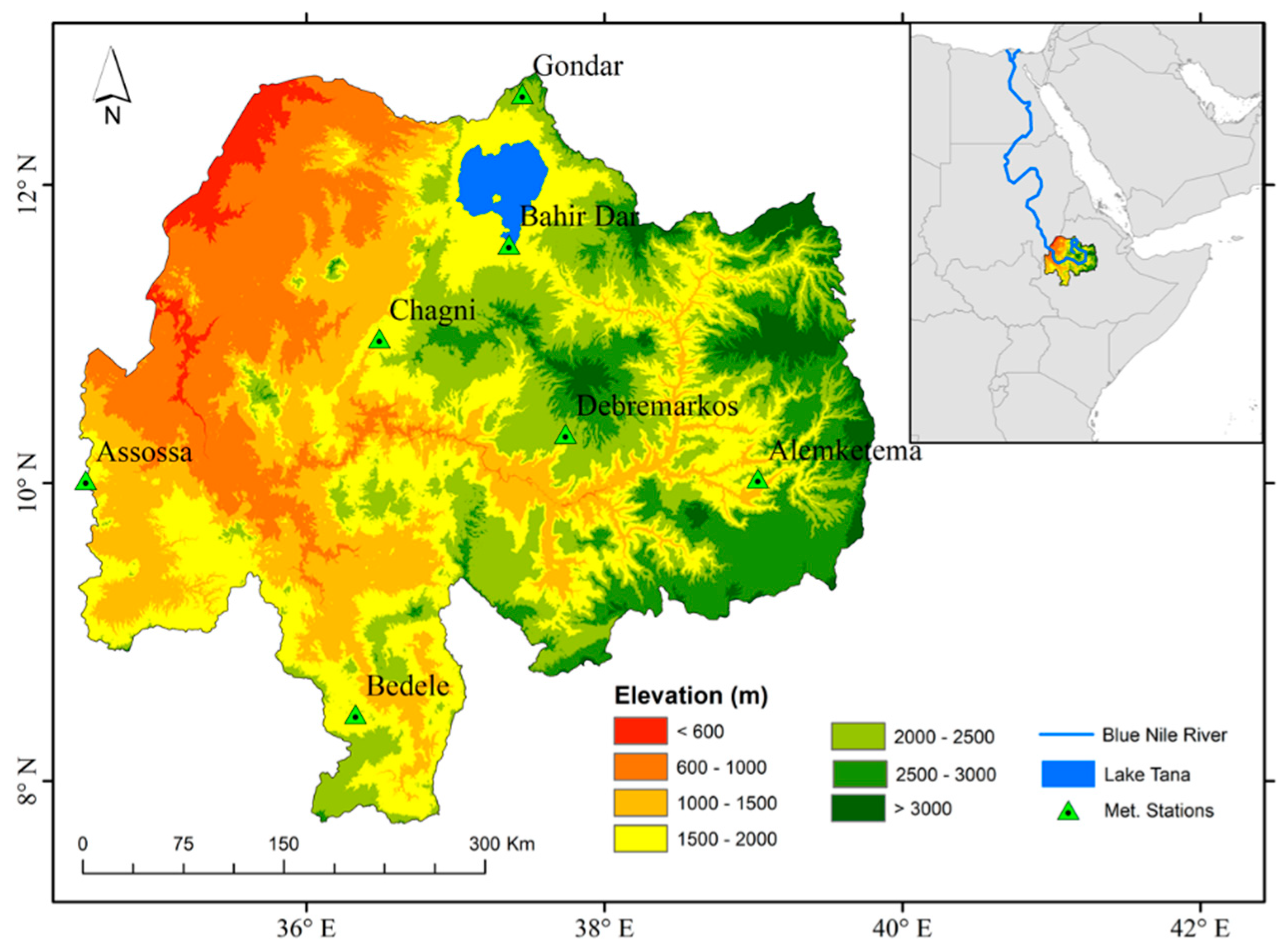
The UBN basin in Ethiopia covers an estimated catchment area of 176,000 [34]. As depicted in Figure 1, it lies approximately between 7°40′ to 12°5′ N and 34°25′ to 39°49′ E. The elevation varies from 483 m at the exit of the Sudanese border to 4261 m above mean sea level (ASL) at Ras Dashen mountain in the north-eastern part of Ethiopia [35]. The 30 m resolution digital elevation model of the NASA Shuttle Radar Topographic Mission (SRTM) (Figure 1) depicts that the highest elevations, exceeding ASL by 4000 m, are centered on the eastern part of the basin and steadily decline in the direction of the western exit of the basin, where the altitude is almost 483 m ASL. The majority of the UBN basin flow occurs between June and September, with the outflow from Lake Tana accounting for about 7% [36].
Teleconnections strongly influence the basin’s climate, with the ENSO as a primary driver of interannual precipitation variability in the basin [37], followed by the Indian Ocean and the Gulf of Guinea [38,39]. El Nino conditions correspond to periods of low precipitation and La Nina conditions correspond to periods of high precipitation [40]. Notably, the January–February sea surface temperatures in the Pacific Ocean have significant correlations with the summer rainfall of the basin [41], whereas a positive Indian Ocean Dipole (IOD) index extends the precipitation season over the basin [42]. Seasonal precipitation forecasts and Blue Nile flow predictions use these teleconnections to analyze the impacts of the oscillating modes of the climate indices [43].
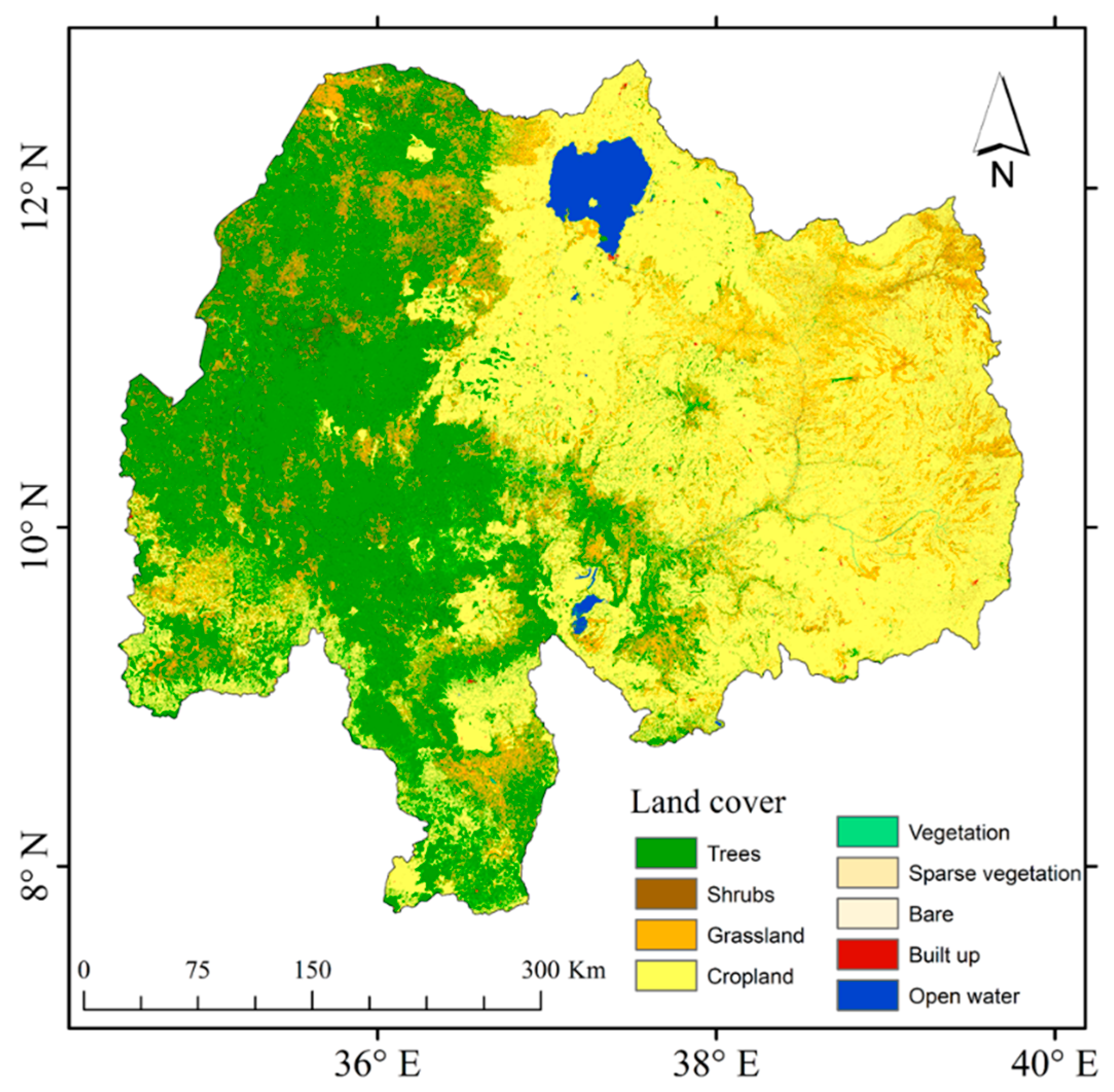
The basin is composed of highlands in the northeastern part and valleys in the southern and western portions [44]. Due to its topography and irregular rainfall distribution, the basin has a mixed land use/cover pattern. Figure 2 shows the land cover types of the basin, extracted from the European Space Agency (2016) global land cover map. The most dominant cover types are cropland, grassland, and trees. Croplands cover 44% of the total area of the basin. Many inhabitants of the basin are engaged in subsistence agriculture, making them vulnerable to prolonged dry conditions [45] and climate extremes, including crop failures due to droughts [46].
2.2. Data Sources
For this study, we considered seven meteorological stations, namely Alemketema, Asossa, Bahir Dar, Bedele, Chagni, Debremarkos, and Gondar, which represent the different climates in the basin. Rainfall and temperature datasets from these metrological stations were collected from the National Metrological Agency of Ethiopia. The rain gauge data were consisted to be mostly of poor quality due to local conditions and instrumentation. Therefore, there was a need to check the consistency and homogeneity of the records made. Double mass curve analysis is an essential tool designed for this purpose. The method is based on the hypothesis that each item of the recorded data is consistent. It produces a double mass curve validating whether the data come from the same population, and thus are consistent. For the selected stations, the double mass curve analysis illustrated that a break in slope was not detected during the study period, and thus the data were reliable and usable enough for evaluation. The seven stations used for this study are presented in Table 1.
There are three main seasons in the basin: the dry season from October to February, the small rain season from March to May, and the main rain season from June to September [47,48]. As shown in Figure 3, the most important season is the main rainy season (locally referred to as Kiremt), which accounts for about three quarters of total annual rainfall. During this season, rain falls over most of the country, except for the south and southeast areas [49]. In the dry and small rain seasons, fewer rainfall events are recorded in the central and eastern parts of the basin. The mean monthly climatological rainfall and climatic water balance pattern revealed distinct seasonality, with wetter summer and cooler winters across all stations.
Besides the monthly rainfall and temperature datasets, we included six climate indices for the development of the ANN model. The Nino sea surface temperature and PDO time-series values were obtained from the US National Center for Atmospheric Research (https://climatedataguide.ucar.edu/climate-data/nino-sst-indices-nino-12-3-34-4-oni-and-tni). The SOI values were acquired from the National Oceanic and Atmospheric Administration (https://www.ncdc.noaa.gov). The IOD index was obtained from the Japan Agency for Marine-Earth Science and Technology (https://www.jamstec.go.jp/frsgc/research/d1/iod/). These data sources are maintained regularly, and no post-processing was carried out.
3. Methodology
3.1. SPEI
The SPEI index, predicted by a “climatic water balance” approach, is multi-scalar, and facilitates drought analysis and monitoring over different time scales. Vicente-Serrano et al. [14] established the method, which takes as input the variation between precipitation and potential evapotranspiration (PET), which is derived from precipitation and temperature datasets.
In our study, subject to data availability, the Thornthwaite [50] method was used to calculate PET. The calculation of PET involves the monthly mean temperature, expressed as
where T is the monthly mean temperature (°C), H is a heat index, which is calculated as the sum of 12 monthly index values that are computed from the mean monthly temperatures, m is a coefficient depending on H , and K is a correction coefficient derived as a function of the latitude and month.
where S is the sum of days of the month and N is the maximum number of sun hours, calculated as
where represents the hourly angle of the sun rising, estimated from the latitude and solar declination [28].
Consequently, the water balance (the surplus or deficit of water) was calculated as
Di values were then aggregated at different time scales. Following the Vicente-Serrano et al. [14] approach, the log-logistic distribution F(x) was applied to transform the original D series into standardized units at different time scales. Finally, the F(x) distribution was utilized to calculate the SPEI following the inverse normal function discussed in Reference [51]. The complete derivation and theory of the index can be found in [52].
In this paper, the SPEI package for R developed by [14] was used to calculate the SPEI drought index. It is a useful research and operational tool for drought analysis. Based on the SPEI values, the levels of drought were categorized as shown in Table 2.
The negative SPEI values indicated drought conditions and were mainly accompanied by a reduction in rainfall, whereas positive values corresponded to wetter or above-normal conditions.
3.2. Artificial Neural Networks (ANNs)
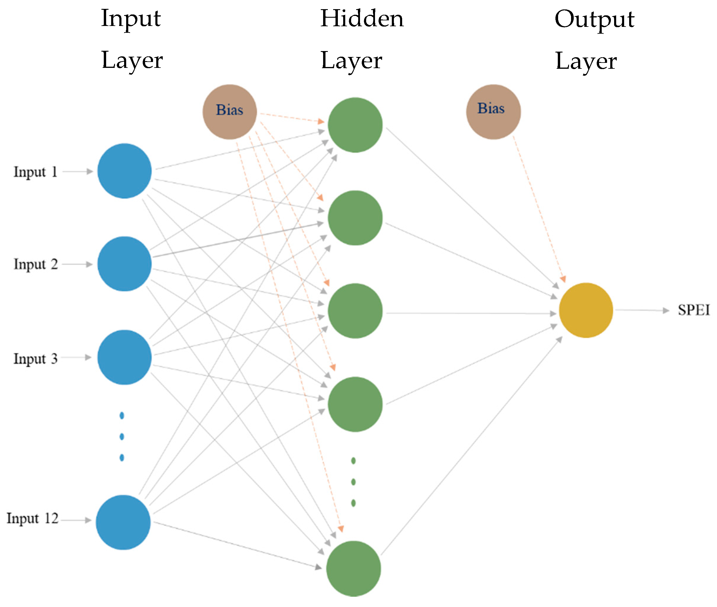
As flexible data-driven models, ANNs have been applied for many functions, such as predictions, curve fitting, and regression in the fields of engineering, earth sciences, medicine, hydrology, etc. [53,54]. ANN models learn data and perform tasks such as classification or prediction. The characteristics of the data are used to determine the network model in the building process, unlike other models that use prior assumptions. ANN structures are organized in layers arranged as input, hidden, and output layers. Within every layer, there are interrelated units known as neurons or nodes.
The ANN models depicted in Figure 4 show a simplified neural network comprising inputs which are multiplied by a modifiable weight. These weights are the crucial parameters of the ANN models used to solve a problem. The sum of the weighted inputs and the bias terms are passed into an activation function that is implemented to prevent the output from becoming too large. Commonly implemented choices of activation functions include the logarithmic sigmoid , tangent sigmoid , linear , and the rectified linear unit (ReLU) functions.
In general, the data presented to the input layer initiate the propagation of information. Subsequently, the network adjusts its weights and uses a learning algorithm to find a combination of weights that yields the smallest error. This process is referred to as “training”. Upon successful accomplishment of the training phase, a new independent testing set is used to validate the trained model. To prevent overfitting, and to generalize better, we used a dropout regularization technique.
3.3. ANN Model Development
In this paper, a multilayer perceptron (MLP) feed-forward network was used to forecast the time-series SPEI at a 12 months time scale. The multilayer perceptron minimized the error between the ANN model outputs and observed values by updating the weights between each node. Amid the pool of the weight-updating process, the resilient back-propagation (RProp algorithm from the “nuerlanet” package in R [55]) was chosen because it can combine fast convergence and stability and generally provides good results [56]. In the modeling of hydrological processes, challenging issues arise from the highly nonlinear nature of the measured variables and their multiple interrelations [57]. To effectively model such large inputs, the selection of appropriate model architecture and the number of hidden neurons and nodes is crucial [58]. The selection of the hidden nodes is the tricky part in ANN modeling. To date, there are no exact guidelines for issues such as how many hidden layers and hidden nodes should be included in an ANN model [59]. Thus, we employed a trial and error approach to find the optimal number of nodes for the hidden layer.
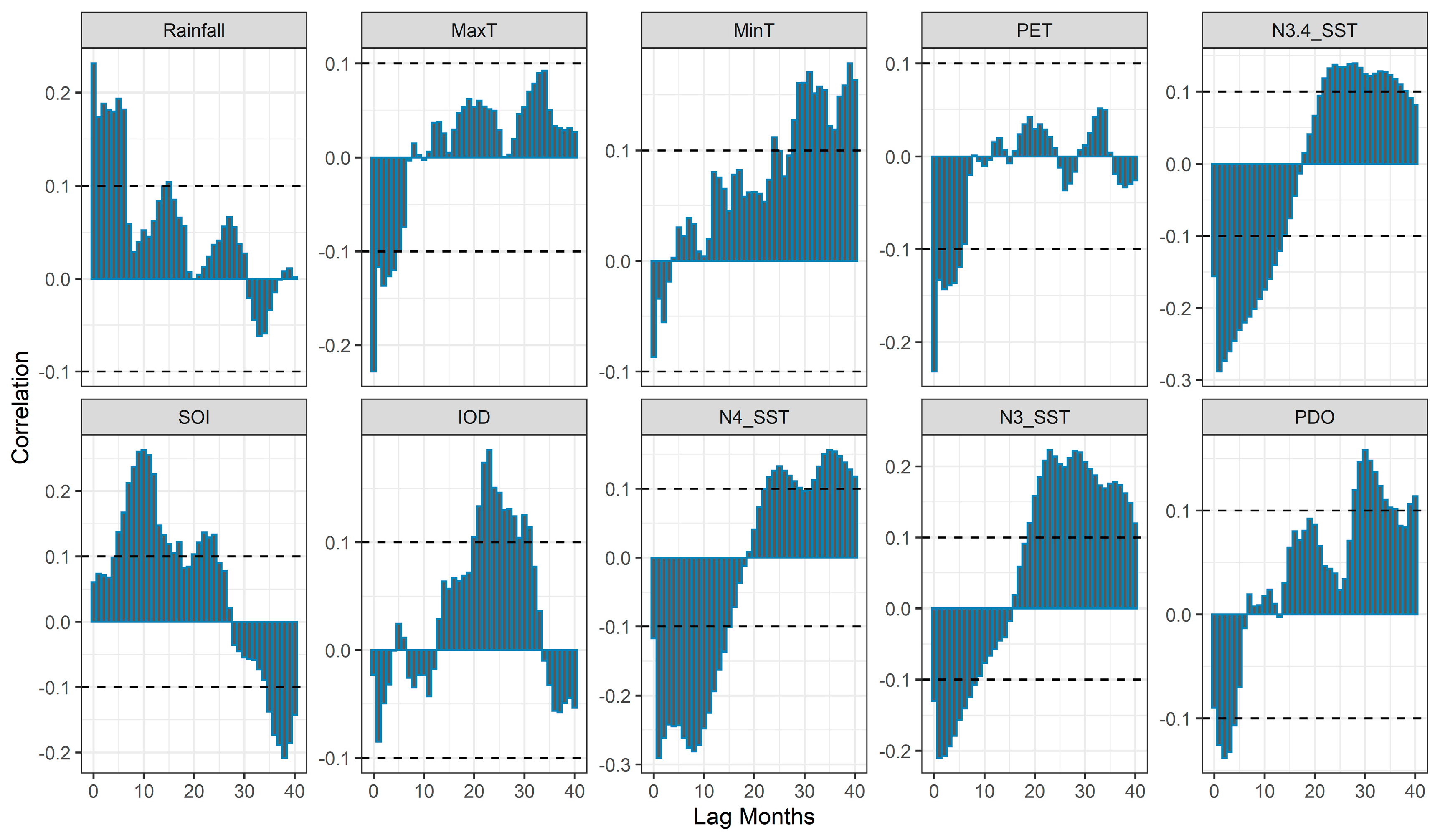
In this paper, we split the data into training and test sets, where the test data were kept out of the process of producing the ANN model in order to test its predictive power. For the period of 1986 to 2015 (30 years), the study area experienced significant changes in rainfall, and thus we chose the years 1986 to 2009 (288 months), precisely 80% of the dataset, for the training set, and from 2010 to 2015 (72 months), i.e., 20% of the dataset, as the testing set. Thus, the results presented in the results section are the estimates of the performance of the ANN on the test data. The climate and SST signals surrounding the study area and hydro-metrological and local variables were considered as predictors. The large-scale potential climate predictors included in the ANN model formulation were the ENSO, IOD, southern oscillation index (SOI), and Pacific decadal oscillation (PDO). According to References [14] and [28], drought predictions are also based on on lags in the impacts of ENSO events. The identification of the time lag between a large-scale climate phenomenon and drought conditions helps to minimize the impacts of ENSO on the region. Thus, a cross-correlation analysis was performed to measure the relationship between the lag times of the potential predictors and the SPEI drought index.
It was evident, as shown in Figure 5, that rainfall and PET had the highest correlations with the SPEI 12 for shorter lag periods. Similarly, Nino indices also had a significant correlation. On the other hand, among the climate signals, significantly positive and negative relationships were observed for IOD and SOI, whereas PDO showed weak relationships with SPEI. Based on the cross-correlations plot shown in Figure 5, seven different ANN models (shown in Table 3) were proposed. Our input selection was based on the outcome of the cross-correlation analysis, i.e., the observed relationships between SPEI and time-lagged climate variables and local variables.
The first model was built using all available data, and, from that, we systematically discarded inputs to compare the accuracy level and the sensitivity of inputs, e.g., by adding and removing climate signals and local variables, etc. In general, this approach helped us to check which models achieved better prediction. The effects of climate signals and local variables were also independently investigated for their value in explaining SPEI variation at different lead times. In general, this systematic selection of input variables aimed to check the sensitivity of input variables in order to arrive at a highly accurate model.
3.4. Statistical Performance Measures
The implementation of the ANN in predicting SPEI values was assessed via the coefficient of determination (R2), root-mean-square error (RMSE), Willmott’s index of agreement (d), and the Nash–Sutcliffe coefficient of efficiency (E). The following mathematical equations define these metrics.
where N is the number of test datasets, Oi is the observed SPEI value, and Pi is the ANN-predicted SPEI value. RMSE was used to measure the average ANN model prediction error to indicate how close the predicted values were to the observed. Lower values of the index indicate high prediction accuracy. The coefficient of determination R2 was determined from the scattered plot of the observed and predicted SPEI values from the fitted regression line. The best model should have an R2 value close to unity. R2 = 1 denotes an exact linear relationship between the observed and predicted values. However, correlation-based measures are oversensitive to extreme values. As a result, a model might appear to be a good predictor when it is not [60]. The Nash–Sutcliffe coefficient of efficiency [61] is 1 minus the absolute difference between the sum of the squared differences between the predicted and observed values, standardized by the variance of the observed values during the study period. The Nash–Sutcliffe coefficient of efficiency (E) statistical measure ranges from −Infinity to 1, and a value closer to unity indicates a better relationship of the observed to the predicted data. However, it has drawbacks, as the errors are calculated as square terms and hence larger values in a time-series are overestimated, whereas lower values are neglected [62]. To overcome the insensitivity of Nash–Sutcliffe coefficient of efficiency (E) and the coefficient of determination (R2), Willmott’s index of agreement (d) was proposed [63]. Willmott’s index of agreement (d) gives a value between 0 and 1, and a value close to unity indicates the realization of the best model, whereas a value close to 0 indicates no agreement at all. The index improves upon those mentioned above, yet remains sensitive to extreme events. For sound scientific model calibration and evaluation, a combination of different performance measures is recommended. The performance of the ANN in terms of the score metrics between the observed SPEI and predicted ANN outputs were examined and the results are presented in the next section. The best ANN architecture was trained with the resilient back-propagation learning algorithm with the tangent sigmoid hidden transfer function. Furthermore, the output transfer function was chosen to be linear.
4. Results and Discussions
4.1. Model Performance
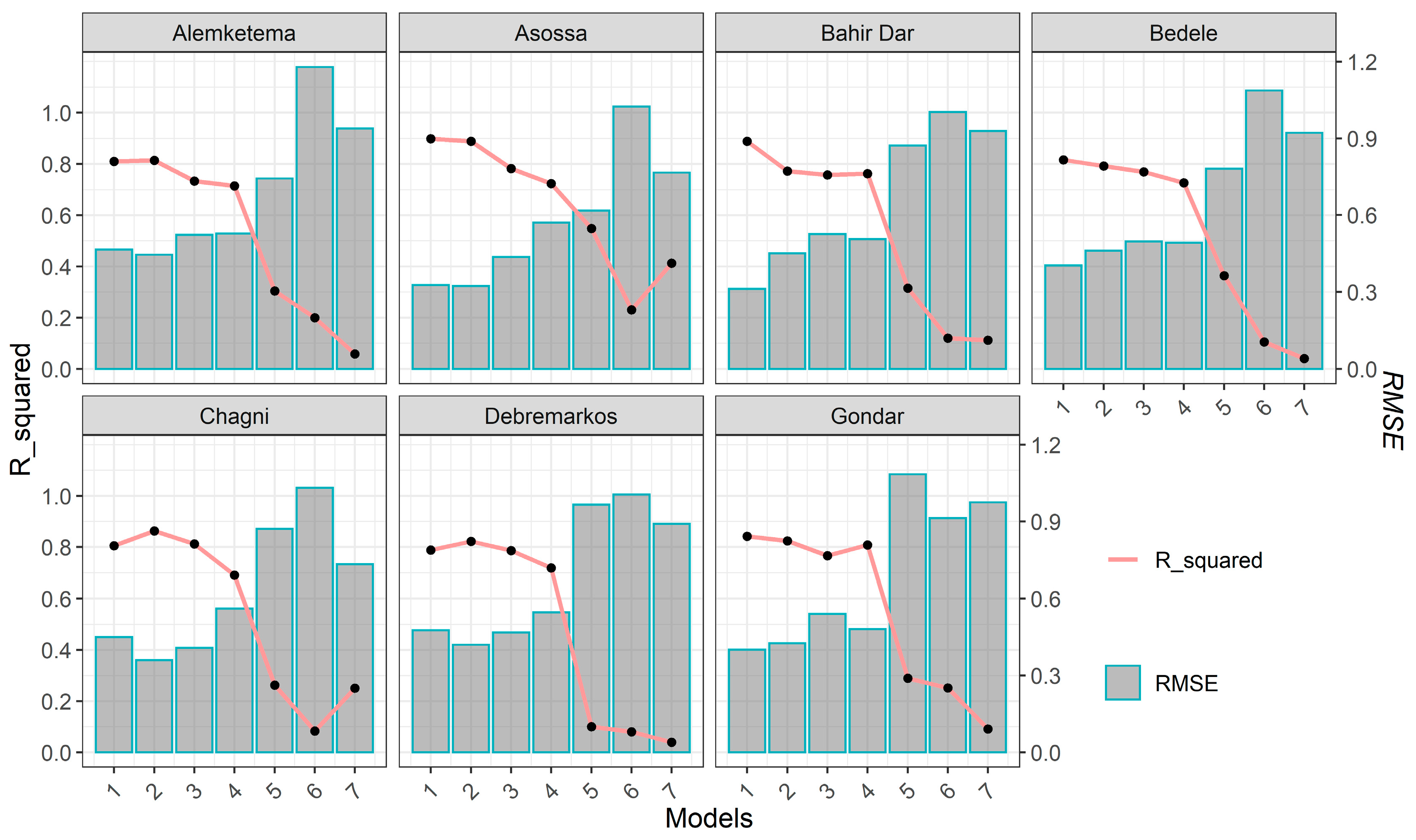
The model performances for predicting time-series SPEI values at different time scales are shown in Figure 6. The seven models, which varied in the scheme of the inputs for predicting the time-series SPEI, displayed significantly different results.
The first four models, which utilized the climate signals, SST indices, and hydro-metrological variables, had an excellent performance at all time scales (high coefficients of determination and low root-mean-square error () values in forecasting the time-series SPEI for all stations, confirming that ANN as a data-driven model was very good at predicting time-series hydrological signatures. However, removing the climate and SST signals (Model 5), hydro-metrological and local variables (Model 6), or local variables, climate, and SST signals (Model 7) resulted in a very weak and low correlation between the observed and forecasted SPEI values. We found that the input variables must be carefully chosen to produce the best model. Model 2, which was built by eliminating the PDO, which had a very weak relationship with the SPEI, as shown in Figure 4, showed a slight improvement over Model 1, although Model 1 still provided a reasonable answer.
We then evaluated the performance of ANN Model 2 in predicting the SPEI 12 values. The best architecture was found to be 11 input layers, 14 hidden layers, and 1 output layer. The quality of the ANN model for the seven stations was examined via statistical performance measures. The measure of the errors was assessed using statistical performance Equations (6)–(9) for all stations, as presented in Table 4 for the test data. Table 4 unveils the averaged model performance statistics for the 72 months in the test dataset as the coefficient of determination (R2), RMSE, Willmott’s index of agreement (d), and the Nash–Sutcliffe coefficient of efficiency (E).
From the results summarized in Table 4, the highest coefficient of determination (0.949) and the smallest RMSE (0.263) was captured at Gondar station. Furthermore, the Willmott’s index of agreement (d = 0.987) and Nash–Sutcliffe coefficient of efficiency (E = 0.949) values for Gondar station were the highest among all the stations. On the other hand, the ANN model resulted in the worst predictions at Bahir Dar station, as it provided a low coefficient of determination (0.82), high RMSE (0.428), low Willmott’s index of agreement (d = 0.946) value, and low Nash–Sutcliffe coefficient of efficiency (E = 0.818) compared to the other stations. In total, the model performance metrics averaged over all stations confirmed that the ANN model performed well in forecasting the drought index.
Another indicator of the quality of model performance is the magnitude of the prediction error (PE), where . This was used to check whether the model overpredicted (PE > 0) or underpredicted (PE < 0) the observed SPEI 12 values. In general, the ideal value of PE is zero. We present the maximum, minimum, and standard deviations of the PE in Table 5. The smallest PE was registered for the Gondar station (PE ≈ 0.690), which was also backed by the predicted and observed SPEI 12 values summarized in Table 4.
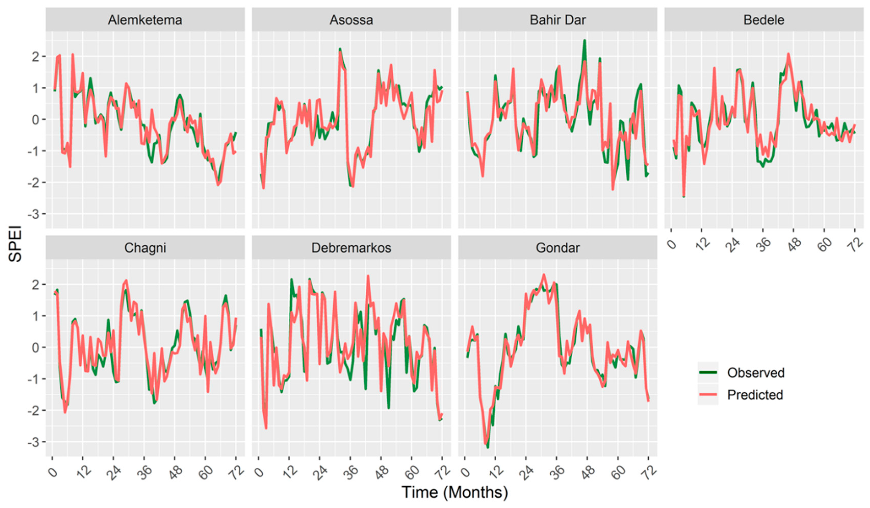
The visual comparison plots of the observed and predicted SPEI values in the test period (2010–2015), shown in Figure 7, provided additional information that the SPEI 12 forecast had less deviation and therefore it was more accurate. The comparison to assess whether the ANN model overpredicted or underpredicted the SPEI 12 values showed significant and substantial differences for Asossa and Bahir Dar stations. The most considerable difference was found for Asossa station, where nearly 59% were underpredicted, whereas approximately 56% were overpredicted for Bahir Dar station.
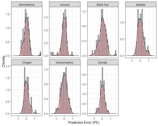
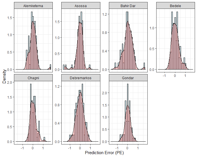
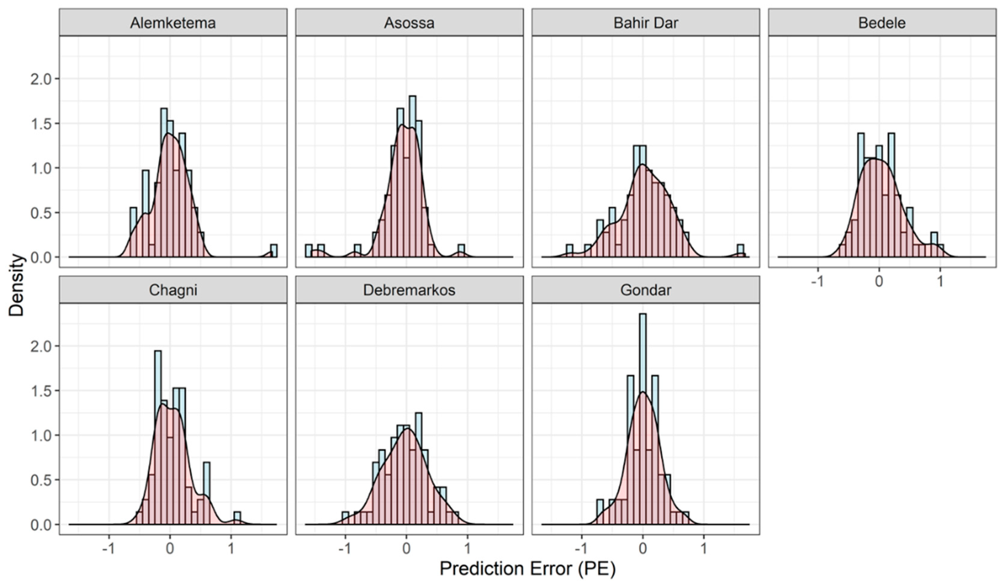
The histogram density plot for the prediction error (PE) in contrast to the normal distributions is presented in Figure 8. The figure demonstrates the underprediction and overprediction by the best ANN model for each of the seven stations. The range of the PE for the Gondar station was the smallest at −0.653 ≤ PE ≤ 0.69. The next best range of the PE was achieved at Chagni station, where it was −0.518 ≤ PE ≤ 1.075.
The underprediction for Alemketema, Bedele, Chagni, and Debremarkos stations was 48.6%, 45.8%, 45.8%, and 51.3% respectively. The overpredictions for Alemketema, Bedele, Chagni, and Debremarkos stations were 51.4%, 54.8%, 54.2%, and 48.7%, respectively. Surprisingly, the overpredictions and underpredictions were equal for Gondar station. We concluded that for all stations, the ANN model predictions showed no systematic errors. The distribution of the PE was thinner and had low standard deviation, which was visually confirmed from its nearly normal distributions.
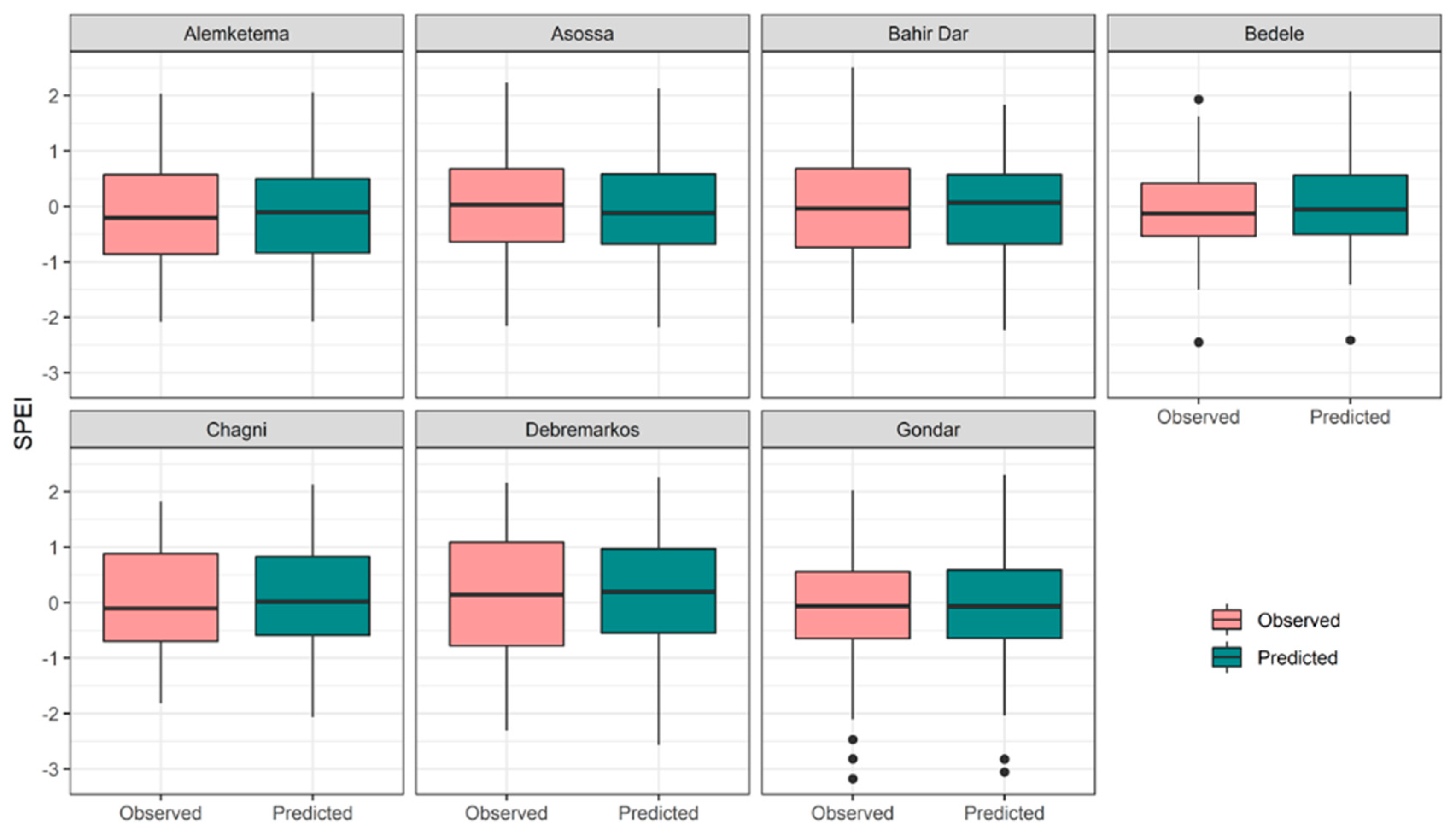
Additionally, box plots provided an excellent review of the distribution of the data and made a comparison of the data more accessible. The box in Figure 9 represents 50% of the data points enclosed by the first and third quartiles. The horizontal line inside the box represents the median value of the dataset. The whisker lines provide us with the range of the data. Additionally, the dots below the minimum and above the maximum SPEI values show the outliers of the data. Note that the figure provides two sets of boxes, one for the observed and the other for the predicted SPEI values. The observed and predicted SPEI values, on average, had a high level of agreement with each other. Given the same range for the whiskers, we interpreted this to mean that the observed and predicted SPEI values varied in the same way. For nearly all stations in this study, the medians were at approximately the same level.
Several approaches have been implemented to assess the strength of the association of a specific explanatory variable for the response variable. Garson’s algorithm, implemented in the NeuralNetTools library [64], was the approach used in this paper. The method assigns a single value to each explanatory variable by deconstructing the weights in the model, which then describes the relationship between the explanatory variable and the response variable [65]. The resulting plot, shown in Figure 10, provided a list of the most significant variables in descending order. Such a figure is an excellent tool for variable selection when there are many variables. The top variables of rainfall, maximum temperature, and potential evapotranspiration contributed more to the ANN model than the bottom ones, and had high predictive power in classifying drought and non-drought events.
4.2. Comparison of Different Models
For comparison, we created two models, a linear model with ordinary least squares and a neural net model with two hidden layers. Standard and simple fitted versus actual, and fitted versus residual plots were used to compare model performance visually. As shown in Figure 11a, the ANN model with two hidden layers had the best performance based on how close the points were to the reference line. The RMSE errors were 0.753, 0.807, and 1.126 for the two-layer ANN, one-layer ANN, and linear models, respectively. The ANN models were far better at predicting new data than the linear model. However, the two-layer model appeared to be slightly better, mainly due to its capacity to capture greater non-linearity.
Though Figure 11a gives a sense that the ANN provided a better result than the ordinary least square model, a more rigorous approach was required to differentiate the neural models. A simulation was run on different segments of the data, namely the 10-fold cross-validation technique. A more precise estimate of the average RMSE results is plotted in Figure 11b. From this plot, we can see a slight difference in the RMSE means of the two ANN models. We conducted a Welch two-sample t-test and found that the p-value = 0.397, with the 95% confidence interval containing zero (−0.3892, 0.0125). From this result, we can say that there was not enough evidence of a difference between the true means of the RMSEs of the two models at a significance level of α = 0.05. The performance of the ANN models did not yield significantly different results, although there were indications that the two-layer layer model performed slightly better.
5. Conclusions
In this study, the UBN basin of Ethiopia was chosen as a study area to build a data-driven ANN model for forecasting the SPEI index. The model was trained by utilizing large-scale climate indices (SOI, IOD, PDO) and SST (Nino 3.0, 3.4, 4.0), which are linked to changes of atmospheric and ocean circulation, and hydro-metrological variables (RF, Max T, Min T, PET,) as the input variables for the ANN model, and the output variables were the SPEI values calculated at a 12 months timescale. Based on the results, we concluded that the best ANN forecasting model built using large-scale climate indices and SST made better predictions, which was verified by analysis of the prediction errors. For all stations, the model returned values that were close to the observed values. The box and histogram plots revealed a high level of similarity between observed and predicted SPEI values. Furthermore, we studied the sensitivity of each predictor variable and found that including the PDO as a predictor variable weakened the quality of the prediction model. Thus, careful assessment needs to made when choosing input variables. Moreover, ANN models developed in this way are easier and less complicated to apply, and can be adapted to various areas to better predict the responses of drought patterns to atmospheric and ocean circulations. Generally, drought forecasting is of great importance in providing information on future drought conditions, which is of particular importance to sustainable agricultural and natural resource management in developing nations, which are directly affected by drought risks in a changing climate. ANNs, as one of the most useful and exciting machine learning algorithms, give access to short- and long-term forecasts that can provide relevant information to maintain sustainable agriculture in both developing and developed countries.
Author Contributions
G.M.M. and Y.-A.L. conceived the research, make helpful discussions during the conception of the research. G.M.M. conducted the research, performed analyses, and wrote the first manuscript draft. Y.-A.L. enhanced and finalized the manuscript for communication with the journal. All authors have read and agreed to the published version of the manuscript.
Funding
This work was supported by the Ministry of Science and Technology under Grant MOST 108-2111-M-008 -036 -MY2 and Grant 108-2923-M-008 -002 -MY3.
Conflicts of Interest
The authors declare no conflict of interest.
References
- Wilhite, D.A.; Glantz, M.H. Understanding: The drought phenomenon: The role of definitions. Water Int. 1985, 10, 111–120. [Google Scholar] [CrossRef] [Green Version]
- Cheng, C.-H.; Nnadi, F.; Liou, Y.-A. Energy budget on various land use areas using reanalysis data in Florida. Adv. Meteorol. 2014, 2014, 1–13. [Google Scholar] [CrossRef] [Green Version]
- Dorjsuren, M.; Liou, Y.-A.; Cheng, C.-H. Time series MODIS and in situ data analysis for Mongolia drought. Remote Sens. 2016, 8, 509. [Google Scholar] [CrossRef] [Green Version]
- Luo, L.; Apps, D.; Arcand, S.; Xu, H.; Pan, M.; Hoerling, M. Contribution of temperature and precipitation anomalies to the California drought during 2012–2015. Geophys. Res. Lett. 2017, 44, 3184–3192. [Google Scholar] [CrossRef]
- Habibi, B.; Meddi, M.; Torfs, P.J.J.F.; Remaoun, M.; Van Lanen, H.A.J. Characterisation and prediction of meteorological drought using stochastic models in the semi-arid Chéliff–Zahrez basin (Algeria). J. Hydrol. Reg. Stud. 2018, 16, 15–31. [Google Scholar] [CrossRef]
- Liou, Y.A.; Nguyen, A.K.; Li, M.H. Assessing spatiotemporal eco-environmental vulnerability by Landsat data. Ecol. Indic. 2017, 80, 52–65. [Google Scholar] [CrossRef] [Green Version]
- Cheng, C.H.; Nnadi, F.; Liou, Y.A. A regional land use drought index for Florida. Remote Sens. 2015, 7, 17149–17167. [Google Scholar] [CrossRef] [Green Version]
- Liou, Y.A.; Mulualem, G.M. Spatio-temporal assessment of drought in Ethiopia and the impact of recent intense droughts. Remote Sens. 2019, 11, 1828. [Google Scholar] [CrossRef] [Green Version]
- Dutra, E.; Magnusson, L.; Wetterhall, F.; Cloke, H.L.; Balsamo, G.; Boussetta, S.; Pappenberger, F. The 2010–2011 drought in the Horn of Africa in ECMWF reanalysis and seasonal forecast products. Int. J. Climatol. 2013, 33, 1720–1729. [Google Scholar] [CrossRef] [Green Version]
- Wu, X.; Hongxing, C.; Flitma, A. Forecasting monsoon precipitation using artificial neural networks. Adv. Atmos. Sci. 2011, 14, 123. [Google Scholar] [CrossRef]
- Wu, C.L.; Chau, K.W.; Li, Y.S. Predicting monthly streamflow using data-driven models coupled with data-preprocessing techniques. Water Resour. Res. 2009, 45. [Google Scholar] [CrossRef] [Green Version]
- Hao, Z.; Singh, V.P.; Xia, Y. Seasonal Drought Prediction: Advances, Challenges, and Future Prospects. Rev. Geophys. 2018, 56, 108–141. [Google Scholar] [CrossRef] [Green Version]
- Zargar, A.; Sadiq, R.; Naser, B.; Khan, F.I. A review of drought indices. Environ. Rev. 2011, 19, 333–349. [Google Scholar] [CrossRef]
- Vicente-Serrano, S.M.; Beguería, S.; López-Moreno, J.I.; Vicente-Serrano, S.M.; Beguería, S.; López-Moreno, J.I. A multiscalar drought index sensitive to global warming: The standardized precipitation evapotranspiration index. J. Clim. 2010, 23, 1696–1718. [Google Scholar] [CrossRef] [Green Version]
- Almedeij, J. Drought analysis for kuwait using standardized precipitation index. Sci. World J. 2014, 2014. [Google Scholar] [CrossRef] [PubMed] [Green Version]
- Yu, C.; Li, C.; Xin, Q.; Chen, H.; Zhang, J.; Zhang, F.; Li, X.; Clinton, N.; Huang, X.; Yue, Y.; et al. Dynamic assessment of the impact of drought on agricultural yield and scale-dependent return periods over large geographic regions. Environ. Model. Softw. 2014, 62, 454–464. [Google Scholar] [CrossRef] [Green Version]
- Hayes, M.J.; Svoboda, M.D.; Wardlow, B.D.; Anderson, M.C.; Kogan, F. Drought monitoring: Historical and current perspectives. In Remote Sensing of Drought: Innovative Monitoring Approaches; CRC Press: Boca Raton, FL, USA, 2012; pp. 1–19. ISBN 9781439835609. [Google Scholar]
- Yusuf, A.A.; Francisco, H. Climate change vulnerability mapping for Southeast Asia vulnerability mapping for Southeast Asia. East 2009, 181, 1–19. [Google Scholar]
- Mishra, S.S.; Nagarajan, R. Forecasting drought in Tel River Basin using feedforward recursive neural network. Int. Conf. Environ. Biomed. Biotechnol. 2012, 41, 122–126. [Google Scholar]
- Pulwarty, R.S.; Sivakumar, M.V. Information systems in a changing climate: Early warnings and drought risk management. Weather Clim. Extrem. 2014, 3, 14–21. [Google Scholar] [CrossRef] [Green Version]
- Khashei, M.; Bijari, M. An artificial neural network (p, d, q) model for timeseries forecasting. Expert Syst. Appl. 2009, 37, 479–489. [Google Scholar] [CrossRef]
- Barua, S.; Ng, A.W.M.; Perera, B.J.C. Artificial Neural Network–Based drought forecasting using a nonlinear aggregated drought index. J. Hydrol. Eng. 2012, 17, 1408–1413. [Google Scholar] [CrossRef]
- Hardwinarto, S.; Aipassa, M. Rainfall monthly prediction based on Artificial Neural Network: A case study in Tenggarong station, East Kalimantan–Indonesia. Procedia Comput. Sci. 2015, 59, 142–151. [Google Scholar] [CrossRef] [Green Version]
- Morid, S.; Smakhtin, V.; Bagherzadeh, K. Drought forecasting using artificial neural networks and time series of drought indices. Int. J. Climatol. 2007, 27, 2103–2111. [Google Scholar] [CrossRef]
- Liou, Y.A.; Liu, S.F.; Wang, W.J. Retrieving soil moisture from simulated brightness temperatures by a neural network. IEEE Trans. Geosci. Remote Sens. 2001, 39, 1662–1672. [Google Scholar]
- Belayneh, A.; Adamowski, J.; Khalil, B. Short-term SPI drought forecasting in the Awash River Basin in Ethiopia using wavelet transforms and machine learning methods. Sustain. Water Resour. Manag. 2016, 2, 87–101. [Google Scholar] [CrossRef]
- Deo, R.C.; Şahin, M. Application of the Artificial Neural Network model for prediction of monthly standardized precipitation and evapotranspiration index using hydrometeorological parameters and climate indices in eastern Australia. Atmos. Res. 2015, 161–162, 65–81. [Google Scholar] [CrossRef]
- Le, M.H.; Perez, G.C.; Solomatine, D.; Nguyen, L.B. Meteorological drought forecasting based on climate signals using Artificial Neural Network—A case study in Khanhhoa Province Vietnam. Procedia Eng. 2016, 154, 1169–1175. [Google Scholar] [CrossRef] [Green Version]
- Schubert, S.D.; Stewart, R.E.; Wang, H.; Barlow, M.; Berbery, E.H.; Cai, W.; Hoerling, M.P.; Kanikicharla, K.K.; Koster, R.D.; Lyon, B.; et al. Global meteorological drought: A synthesis of current understanding with a focus on SST drivers of precipitation deficits. J. Clim. 2016, 29, 3989–4019. [Google Scholar] [CrossRef] [Green Version]
- Roundy, J.K.; Wood, E.F.; Roundy, J.K.; Wood, E.F. The attribution of land–Atmosphere interactions on the seasonal predictability of drought. J. Hydrometeorol. 2015, 16, 793–810. [Google Scholar] [CrossRef]
- Lyon, B. Seasonal drought in the greater horn of Africa and its recent increase during the March–May long rains. J. Clim. 2014, 27, 7953–7975. [Google Scholar] [CrossRef]
- Hoell, A.; Funk, C.; Hoell, A.; Funk, C. The ENSO-related West Pacific Sea surface temperature gradient. J. Clim. 2013, 26, 9545–9562. [Google Scholar] [CrossRef]
- Behrangi, A.; Nguyen, H.; Granger, S. Probabilistic seasonal prediction of meteorological drought using the bootstrap and multivariate information. J. Appl. Meteorol. Climatol. 2015, 54, 1510–1522. [Google Scholar] [CrossRef]
- Allam, M.M.; Jain Figueroa, A.; McLaughlin, D.B.; Eltahir, E.A.B. Estimation of evaporation over the upper Blue Nile basin by combining observations from satellites and river flow gauges. Water Resour. Res. 2016, 52, 644–659. [Google Scholar] [CrossRef] [Green Version]
- Tekleab, S.; Mohamed, Y.; Uhlenbrook, S. Hydro-climatic trends in the Abay/Upper Blue Nile basin, Ethiopia. Phys. Chem. Earth, Parts A/B/C 2013, 61–62, 32–42. [Google Scholar] [CrossRef]
- Samy, A.; Ibrahim, M.G.; Mahmod, W.E.; Fujii, M.; Eltawil, A.; Daoud, W. Statistical assessment of rainfall characteristics in Upper Blue Nile Basin over the period from 1953 to 2014. Water 2019, 11, 468. [Google Scholar] [CrossRef] [Green Version]
- Broman, D.; Rajagopalan, B.; Hopson, T.; Gebremichael, M. Spatial and temporal variability of East African Kiremt season precipitation and large-scale teleconnections. Int. J. Climatol. 2020, 40, 1241–1254. [Google Scholar] [CrossRef]
- Giannini, A.; Biasutti, M.; Held, I.M.; Sobel, A.H. A global perspective on African climate. Clim. Chang. 2008, 90, 359–383. [Google Scholar] [CrossRef]
- Siam, M.S.; Wang, G.; Demory, M.E.; Eltahir, E.A.B. Role of the Indian Ocean sea surface temperature in shaping the natural variability in the flow of Nile River. Clim. Dyn. 2014, 43, 1011–1023. [Google Scholar] [CrossRef]
- Diro, G.T.; Grimes, D.I.F.; Black, E. Teleconnections between Ethiopian summer rainfall and sea surface temperature: Part II. Seasonal forecasting. Clim. Dyn. 2011, 37, 121–131. [Google Scholar] [CrossRef]
- Alhamshry, A.; Fenta, A.A.; Yasuda, H.; Shimizu, K.; Kawai, T. Prediction of summer rainfall over the source region of the Blue Nile by using teleconnections based on sea surface temperatures. Theor. Appl. Climatol. 2019, 137, 3077–3087. [Google Scholar] [CrossRef]
- Segele, Z.T.; Lamb, P.J.; Leslie, L.M. Seasonal-to-Interannual variability of Ethiopia/Horn of Africa monsoon. Part I: Associations of wavelet-filtered large-scale atmospheric circulation and global sea surface temperature. J. Clim. 2009, 22, 3396–3421. [Google Scholar] [CrossRef]
- Berhane, F.; Zaitchik, B.; Dezfuli, A. Subseasonal analysis of precipitation variability in the Blue Nile River Basin. J. Clim. 2014, 27, 325–344. [Google Scholar] [CrossRef]
- Gebremicael, T.G.; Mohamed, Y.A.; Betrie, G.D.; van der Zaag, P.; Teferi, E. Trend analysis of runoff and sediment fluxes in the Upper Blue Nile basin: A combined analysis of statistical tests, physically-based models and landuse maps. J. Hydrol. 2013, 482, 57–68. [Google Scholar] [CrossRef]
- Coffel, E.D.; Keith, B.; Lesk, C.; Horton, R.M.; Bower, E.; Lee, J.; Mankin, J.S. Future hot and dry years worsen Nile basin water scarcity despite projected precipitation increases. Earth’s Futur. 2019, 7, 967–977. [Google Scholar] [CrossRef] [Green Version]
- Broad, K.; Agrawala, S. The Ethiopia food crisis—Uses and limits of climate forecasts. Science 2000, 289, 1693–1694. [Google Scholar]
- Conway, D. The climate and hydrology of the Upper Blue Nile river. Geogr. J. 2000, 166, 49–62. [Google Scholar] [CrossRef] [Green Version]
- Wagesho, N.; Goel, N.K.; Jain, M.K. Temporal and spatial variability of annual and seasonal rainfall over Ethiopia. Hydrol. Sci. J. 2013, 58, 354–373. [Google Scholar] [CrossRef]
- Mellander, P.-E.; Gebrehiwot, S.G.; Gärdenäs, A.I.; Bewket, W.; Bishop, K. Summer rains and dry seasons in the upper blue Nile Basin: The predictability of half a century of past and future spatiotemporal patterns. PLoS ONE 2013, 8, e68461. [Google Scholar] [CrossRef] [Green Version]
- Thornthwaite, C.W. An approach toward a rational classification of climate. Geogr. Rev. 1948, 38, 55. [Google Scholar] [CrossRef]
- Barton, D.E.; Abramovitz, M.; Stegun, I.A. Handbook of mathematical functions with formulas, graphs and mathematical tables. J. R. Stat. Soc. Ser. A 1965, 128, 593. [Google Scholar] [CrossRef] [Green Version]
- Beguería, S.; Vicente-Serrano, S.M.; Reig, F.; Latorre, B. Standardized precipitation evapotranspiration index (SPEI) revisited: Parameter fitting, evapotranspiration models, tools, datasets and drought monitoring. Int. J. Climatol. 2014, 34, 3001–3023. [Google Scholar] [CrossRef] [Green Version]
- Seo, Y.; Kim, S. River stage forecasting using wavelet packet decomposition and data-driven models. Procedia Eng. 2016, 154, 1225–1230. [Google Scholar] [CrossRef] [Green Version]
- Schuman, C.D.; Birdwell, J.D. Dynamic Artificial Neural Networks with affective systems. PLoS ONE 2013, 8, e80455. [Google Scholar] [CrossRef] [PubMed]
- Günther, F.; Fritsch, S. neuralnet: Training of neural networks. R J. 2010, 2, 30–38. [Google Scholar] [CrossRef] [Green Version]
- Riedmiller, M.; Riedmiller, M.; Braun, H. A direct adaptive method for faster backpropagation learning: The rprop algorithm. IEEE Int. Conf. Neural Netw. 1993, 16, 586–591. [Google Scholar]
- Remesan, R.; Mathew, J. Hydrological Data Driven Modelling: A Case Study Approach; Springer International Pu: New York City, NY, USA, 2016; ISBN 9783319092355. [Google Scholar]
- Sheela, K.G.; Deepa, S.N. Review on methods to fix number of hidden neurons in neural networks. Math. Probl. Eng. 2013, 2013. [Google Scholar] [CrossRef] [Green Version]
- Stathakis, D. How many hidden layers and nodes? Int. J. Remote Sens. 2009, 30, 2133–2147. [Google Scholar] [CrossRef]
- Legates, D.R.; McCabe, G.J. Evaluating the use of “goodness-of-fit” Measures in hydrologic and hydroclimatic model validation. Water Resour. Res. 1999, 35, 233–241. [Google Scholar] [CrossRef]
- Nash, J.E.; Sutcliffe, J. V River flow forecasting through conceptual models part I—A discussion of principles. J. Hydrol. 1970, 10, 282–290. [Google Scholar] [CrossRef]
- Krause, P.; Boyle, D.P.; Bäse, F. Comparison of different efficiency criteria for hydrological model assessment. Adv. Geosci. 2005, 5, 89–97. [Google Scholar] [CrossRef] [Green Version]
- Willmott, C.J. On the validation of models. Phys. Geogr. 1981, 2, 184–194. [Google Scholar] [CrossRef]
- Beck, M.W. NeuralNetTools: Visualization and analysis tools for neural networks. J. Stat. Softw. 2018, 85, 1. [Google Scholar] [CrossRef] [PubMed]
- Garson, G.D. A comparison of neural network and expert systems algorithms with common multivariate procedures for analysis of social science data. Soc. Sci. Comput. Rev. 1991, 9, 399–434. [Google Scholar] [CrossRef]
Figure 1.
The geographical location of the Upper Blue Nile (UBN) river basin and metrological stations used in this study.
Figure 1.
The geographical location of the Upper Blue Nile (UBN) river basin and metrological stations used in this study.

Figure 2.
Land cover map of the UBN river basin in 2016 at 20 m spatial resolution, extracted from the European Space Agency.
Figure 2.
Land cover map of the UBN river basin in 2016 at 20 m spatial resolution, extracted from the European Space Agency.

Figure 3.
Monthly climatology of rainfall and climatic water balance, CWBi = Pi − PETi (precipitation − potential evapotranspiration) for the 1986–2015 period.
Figure 3.
Monthly climatology of rainfall and climatic water balance, CWBi = Pi − PETi (precipitation − potential evapotranspiration) for the 1986–2015 period.

Figure 4.
Artificial neural network general architecture.

Figure 5.
Cross-correlation between predictor variables with SPEI 12 at Gondar station.

Figure 6.
Comparison of performance of the seven models at a 12 months time scale.

Figure 7.
Observed and predicted SPEI 12 values using the ANN model.

Figure 8.
Density plots and histograms of the prediction error (PE) values calculated for the test period.
Figure 8.
Density plots and histograms of the prediction error (PE) values calculated for the test period.

Figure 9.
Box plots of the observed and predicted SPEI values plotted for the test period.

Figure 10.
Variable importance plot from the ANN model.

Figure 11.
(a) A scatterplot of the observed versus predicted plots for the two-layer ANN (ANN_2), one-layer ANN (ANN_1), and linear models (LM) with a 1:1 reference line plot. (b) The 10-fold cross-validation root-mean-square errors for the two-layer ANN and one-layer ANN models.
Figure 11.
(a) A scatterplot of the observed versus predicted plots for the two-layer ANN (ANN_2), one-layer ANN (ANN_1), and linear models (LM) with a 1:1 reference line plot. (b) The 10-fold cross-validation root-mean-square errors for the two-layer ANN and one-layer ANN models.


Table 1.
Meteorological stations and their descriptive statistics.
| Station Name | Geographical Locations | Elevation ASL | Annual Mean Rainfall (mm) | Mean Annual Temperature (°C) |
|---|---|---|---|---|
| Alemketema | 10.03° N, 39.03° E | 2280 m | 1049.16 | 19.74 |
| Asossa | 10.02° N, 34.52° E | 1590 m | 1198.57 | 24.61 |
| Bahir Dar | 11.59° N, 37.38° E | 1770 m | 1387.37 | 20.43 |
| Bedele | 8.45° N, 36.33° E | 2030 m | 1809.18 | 17.92 |
| Chagni | 10.97° N, 36.5° E | 1620 m | 1699.58 | 20.34 |
| Debremarkos | 10.33° N, 37.74° E | 2515 m | 1334.15 | 16.27 |
| Gondar | 12.61° N, 37.45° E | 1967 m | 1145.87 | 19.89 |
Table 2.
Drought characterization based on standardized precipitation evapotransporation index (SPEI) values.
Table 2.
Drought characterization based on standardized precipitation evapotransporation index (SPEI) values.
| SPEI Values | Drought Category |
|---|---|
| SPEI ≥ 2 | Extremely wet |
| 1.5 ≤ SPEI < 1 | Severely wet |
| 1 ≤ SPEI < 1.5 | Moderately wet |
| −1 ≤ SPEI < 1 | Near normal |
| −1.5 ≤ SPEI < −1 | Moderately dry |
| −2 ≤ SPEI < −1.5 | Severely dry |
| SPEI < −2 | Extremely dry |
Table 3.
Input variables proposed in the search for suitable models for predicting SPEI.
| Model | No. of Input Variables | Year | Month | Rainfall | Max T | Min T | PET | SOI | IOD | PDO | N3 SST | N3.4 SST | N4 SST |
|---|---|---|---|---|---|---|---|---|---|---|---|---|---|
| M1 | 12 | ✓ | ✓ | ✓ | ✓ | ✓ | ✓ | ✓ | ✓ | ✓ | ✓ | ✓ | ✓ |
| M2 | 11 | ✓ | ✓ | ✓ | ✓ | ✓ | ✓ | ✓ | ✓ | ✓ | ✓ | ✓ | |
| M3 | 10 | ✓ | ✓ | ✓ | ✓ | ✓ | ✓ | ✓ | ✓ | ✓ | ✓ | ||
| M4 | 8 | ✓ | ✓ | ✓ | ✓ | ✓ | ✓ | ✓ | ✓ | ||||
| M5 | 6 | ✓ | ✓ | ✓ | ✓ | ✓ | ✓ | ||||||
| M6 | 6 | ✓ | ✓ | ✓ | ✓ | ✓ | ✓ | ||||||
| M7 | 4 | ✓ | ✓ | ✓ | ✓ |
Table 4.
A measure of ANN model performance based on all statistical measures of the observed SPEI and predicted SPEI.
Table 4.
A measure of ANN model performance based on all statistical measures of the observed SPEI and predicted SPEI.
| Station Name | R2 | RMSE | d | E |
|---|---|---|---|---|
| Alemketema | 0.870 | 0.335 | 0.965 | 0.863 |
| Asossa | 0.892 | 0.349 | 0.966 | 0.884 |
| Bahir Dar | 0.820 | 0.428 | 0.946 | 0.818 |
| Bedele | 0.856 | 0.338 | 0.959 | 0.854 |
| Chagni | 0.908 | 0.290 | 0.975 | 0.905 |
| Debremarkos | 0.865 | 0.363 | 0.964 | 0.862 |
| Gondar | 0.949 | 0.263 | 0.987 | 0.949 |
| Overall station average | 0.880 | 0.338 | 0.966 | 0.876 |
Table 5.
The maximum, minimum, and standard deviation values of the prediction error (PE).
| Station Name | Maximum PE | Minimum PE | Standard Deviation |
|---|---|---|---|
| Alemketema | 1.674 | −0.631 | 0.337 |
| Asossa | 0.877 | −1.561 | 0.346 |
| Bahir Dar | 1.614 | −1.189 | 0.430 |
| Bedele | 0.956 | −0.588 | 0.338 |
| Chagni | 1.075 | −0.518 | 0.288 |
| Debremarkos | 0.799 | −0.964 | 0.364 |
| Gondar | 0.690 | −0.653 | 0.265 |
© 2020 by the authors. Licensee MDPI, Basel, Switzerland. This article is an open access article distributed under the terms and conditions of the Creative Commons Attribution (CC BY) license (http://creativecommons.org/licenses/by/4.0/).
Share and Cite
MDPI and ACS Style
Mulualem, G.M.; Liou, Y.-A. Application of Artificial Neural Networks in Forecasting a Standardized Precipitation Evapotranspiration Index for the Upper Blue Nile Basin. Water 2020, 12, 643. https://doi.org/10.3390/w12030643
AMA Style
Mulualem GM, Liou Y-A. Application of Artificial Neural Networks in Forecasting a Standardized Precipitation Evapotranspiration Index for the Upper Blue Nile Basin. Water. 2020; 12(3):643. https://doi.org/10.3390/w12030643
Chicago/Turabian StyleMulualem, Getachew Mehabie, and Yuei-An Liou. 2020. "Application of Artificial Neural Networks in Forecasting a Standardized Precipitation Evapotranspiration Index for the Upper Blue Nile Basin" Water 12, no. 3: 643. https://doi.org/10.3390/w12030643
Note that from the first issue of 2016, this journal uses article numbers instead of page numbers. See further details here.