Deriving a Bayesian Network to Assess the Retention Efficacy of Riparian Buffer Zones

1
Leibniz-Institute of Freshwater Ecology and Inland Fisheries, 12489 Berlin, Germany
2
Center for Agricultural Technology Augustenberg, 76227 Karlsruhe, Germany
3
Faculty of Biology, Department of Aquatic Ecology, University of Duisburg-Essen, 45141 Essen, Germany
4
Department of Geography, Humboldt-University of Berlin, 12489 Berlin, Germany
*
Author to whom correspondence should be addressed.
Water 2020, 12(3), 617; https://doi.org/10.3390/w12030617
Submission received: 7 January 2020
/
Revised: 7 February 2020
/
Accepted: 11 February 2020
/
Published: 25 February 2020
(This article belongs to the Special Issue Monitoring, Modelling and Management of Water Quality)
Abstract
:Bayesian networks (BN) have increasingly been applied in water management but not to estimate the efficacy of riparian buffer zones (RBZ). Our methodical study aims at evaluating the first BN to predict the RBZ efficacy to retain sediment and nutrients (dissolved, total, and particulate nitrogen and phosphorus) from widely available variables (width, vegetation, slope, soil texture, flow pathway, nutrient form). To evaluate the influence of parent nodes and how the number of states affects prediction errors, we used a predefined general BN structure, collected 580 published datasets from North America and Europe, and performed classification tree analyses and multiple 10-fold cross-validations of different BNs. These errors ranged from 0.31 (two output states) to 0.66 (five states). The outcome remained unchanged without the least influential nodes (flow pathway, vegetation). Lower errors were achieved when parent nodes had more than two states. The number of efficacy states influenced most strongly the prediction error as its lowest and highest states were better predicted than intermediate states. While the derived BNs could support or replace simple design guidelines, they are limited for more detailed predictions. More representative data on vegetation or additional nodes like preferential flow will probably improve the predictive power.
1. Introduction
The eutrophication of lakes and rivers remain a global concern despite considerable efforts in the past to reduce the input of nutrients from terrestrial environments [1]. After targeting the industrial and domestic sources, the diffuse agricultural inputs of nitrogen (N), phosphorus (P), sediments, and also pesticides gained importance [2,3,4,5]. Particularly, the legacy of long-term excess applications of fertilizers and manure became eminent [6,7]. In the European Union (EU), for instance, diffuse sources affect now more water bodies than point sources [8].
Many processes and factors control the mobilization and the diffuse transport of agricultural pollutants. Accordingly, various “best management practices” (BMP) can contribute to reduce the risk of pollutants entering water bodies. Riparian buffers zones (RBZ), also termed vegetated buffer strips, are vegetated areas along water bodies which are either too difficult to work or intentionally set aside [9]. RBZ stand among the most widely applied BMP to reduce the diffuse pollution of surface waters but also to improve their hydro-morphological and thermal conditions [9,10,11]. This is reflected by the rich literature on the efficacy of RBZ to retain substances from adjacent upslope areas (henceforth catchments).
The RBZ efficacy is expressed as the ratio of the amount of nutrients, pesticides, or sediment leaving the buffer towards the water body and the amount of material entering the RBZ from the catchment. It depends on RBZ properties and external factors like land management which, in turn, determine the runoff and incoming nutrients [12,13]. The large variability in RBZ efficacy reported in the literature reflects the variability of those factors.
Therefore, modelling approaches to predict RBZ efficacy in large-scale applications tend to be (too) data-demanding, e.g., process-based models like VFSMOD [14] and REMM [15], or (too) simplistic [16]. For instance, Weissteiner et al. [17] used RBZ width as single variable to estimate the efficacy of N and P retention in their model for the EU. This approach is in line with regulations and recommendations on RBZ design which specify adequate widths of RBZ as simple, easily administrable rules to reduce diffuse emissions of nutrients and sediments [18,19,20]. However, the use of RBZ width as the only design variable is not commonly considered sufficient [21,22].
Some studies used sub-datasets and applied multivariate regression to improve the model performance. For example, Zhang et al. [13] derived separate models for different vegetation types (grass and mixed, only trees), again only with RBZ width as the single explanatory variable for N and P retention. For sediment retention, they considered RBZ slope as the second variable which was supported by a previous study that identified RBZ width and slope to be best correlated with sediment retention [23]. In contrast, Yuan et al. [24] found only a weak relationship between sediment retention and slope. In their meta-analysis on nitrate retention, Mayer et al. [25] also tested RBZ width as the only predictor in regression models for different width classes, vegetation types, and flow pathways. The explained variability (r²) in these subsets was partly higher than the r² values for the full dataset. They concluded that more factors need to be considered. In accordance, Hassanzadeh et al. [16] achieved even higher r² values by considering various RBZ and external variables in their regression model.
Nonetheless, such regression models have limitations which can be addressed by Bayesian networks (BN, also termed Bayesian belief networks, [26]). Firstly, BN explicitly deal with the uncertainty in data or conditions because they represent the relationships (links or edges) between system variables (nodes) probabilistically rather than deterministically [27]. Secondly, they can integrate even incomplete quantitative and qualitative information (e.g., “sandy soil”) from different domains such as expert knowledge, field data, and other BN. Thirdly, BN can provide information on causes from evidence of observed effects.
Although BN have increasingly been applied for water resource management, decision-making, predictions, and assessments of ecosystem services during the last decades [26,28,29,30], they have only implicitly considered RBZ retention so far [31]. Therefore, the aims of this study are (i) to develop the first BN to predict RBZ efficacy to retain N and P from RBZ and external factors, (ii) to train and cross-validate the BN based on empirical data compiled from an extensive literature review, and (iii) to evaluate how node selection and the number of their states, i.e., data discretization, affect model accuracy. As our BN aims at medium- to large-scale applications, we focused on commonly available input data and grouped nutrient fractions of N and P.
2. Materials and Methods
2.1. Data Collection and Preprocessing
We compiled the measured RBZ efficacy for N, P, and sediment and information on generally available RBZ and external variables (first column in Table 1) based on 23 reviews published between 1994 and 2019 [12,13,22,23,24,25,32,33,34,35,36,37,38,39,40,41,42,43,44,45,46,47,48] (Supplementary Table S1). These variables were selected based on key processes of nutrient and sediment retention discussed in the literature, e.g.,
- RBZ width and nutrient form: after entering the RBZ, the velocity of surface runoff decreases due to surface roughness and soil infiltration [22,49,50]. This results in a lower transport capacity and a deposition of sediment and particulate nutrients, which is an important process for their retention [40]. Positive yet variable relationships of RBZ width and efficacy have widely been acknowledged in reviews and guidelines (e.g., [19,33,48]) with broader RBZ being needed to efficiently retain dissolved nutrients compared to sediment [46].
- RBZ vegetation, flow pathway, and nutrient form: dense aboveground vegetation increases the hydraulic roughness and reduces the transport capacity of water for particles, while dense root systems favor soil permeability, porosity, infiltration, and, thus, the sorption of dissolved nutrients (DN, DP) to soil particles as well as their uptake by plants [45,51]. Previous studies reported contrasting results in respect to the efficacy of grassed and woody RBZ [12,52,53]. Most probably, this is due the large number of processes and complex interactions among nutrients, plants, soil, and micro-organisms [54].
- Soil texture, flow pathway, and nutrient form: the larger the soil particles, the faster they settle under given flow conditions. While most of the coarse sediment can be retained even in narrow RBZ, the retention of fine sediment requires soil infiltration in RBZ which are more than 15–20 m wide in order to be effective [12,23,55]. In addition, soil composition (e.g., texture) is decisive for P sorption, hydraulic conductivity and, thus, for surface runoff, soil moisture storage, as well as residence time of nutrients in the root zone [40,47,51,56,57]. While sandy soils favor infiltration, surface flow predominates on clayey soils.
- RBZ slope and width: RBZ are expected to be less effective in reducing the transport capacity of water flow as well as in trapping sediments and nutrients in steep terrain [13,23,40] thus requiring broader buffers on steeper slopes [48]. Due to the experimental design and data availability, the influence of slope was not significant in other studies (e.g., [47,58]). RBZ slope was used in some regression models as an independent variable (e.g., [13,48]).
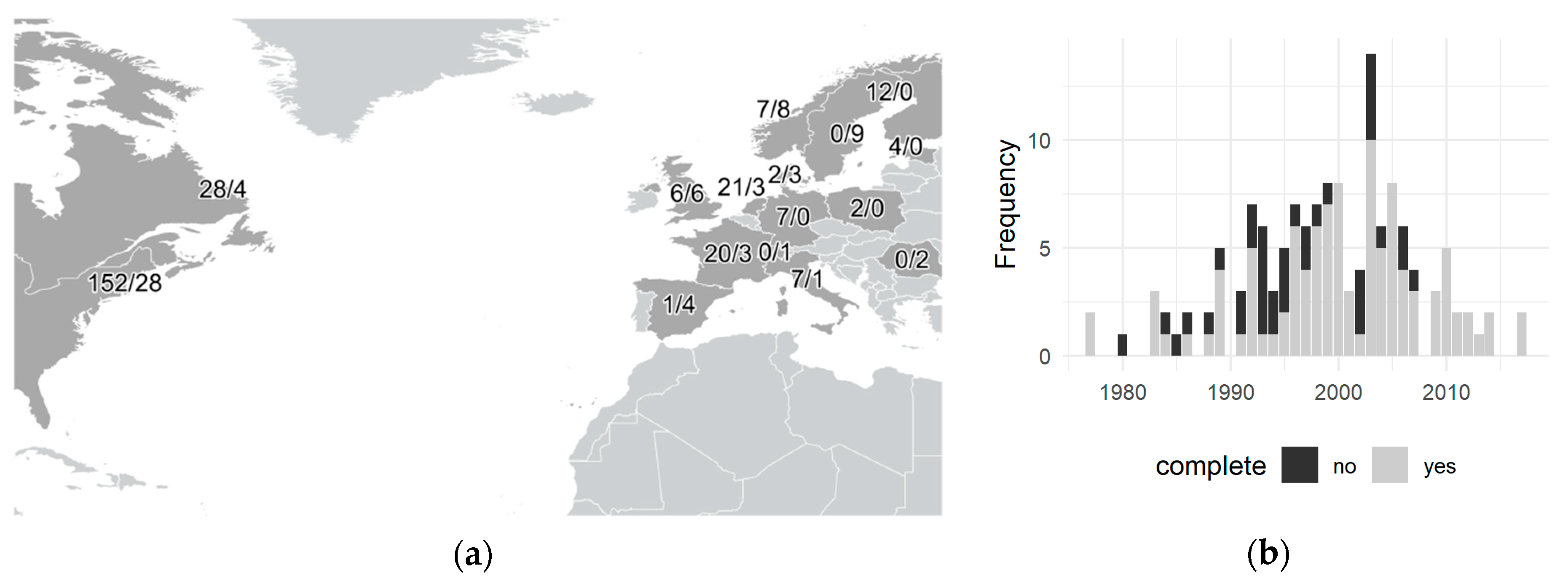
As far as possible, the measured RBZ efficacy values—preferably from mass (load or yield)—were extracted from the original studies to minimize compilation errors and to avoid double counting. From 139 studies, published between 1977 and 2017 (Figure 1b), we gathered 341 datasets with at least one efficacy value mainly located in North America and Western Europe (Figure 1a). Data from other continents as well as model outcomes, (constructed) wetlands, and ponds were not considered.
A total of 269 of the collected datasets were complete, i.e., with values for all variables shown in Table 1 (Table 2). The others missed RBZ slope (n = 52) and soil texture (n = 61). Slope was missing for 39 groundwater studies, i.e., 27% of all, thus shifting the dataset towards studies on surface flow. To increase the sample size, we calculated missing average values from ranges, e.g., the minimum and maximum efficacy given for RBZ of 10–15 m width was converted to an average value of 12.5 m width, and applied no quality criteria apart from data completeness.
Two thirds of the 580 efficacy values with complete data originated from plot studies and one third from field and watershed studies, with different experimental designs and time scales. Rainfall data was particularly inconsistently reported, e.g., as average values or intensities, and was therefore excluded from the data collection.
2.2. Aggregating the Nutrient Forms
We collected the efficacies for five nutrient forms and sediment. In order to reduce the number of states and increase the number of data sets for each state, we applied preliminary regression analyses to quantify the similarity of RBZ efficacy for particulates (mostly sediment) and total N and P (TN, TP) as well as the dissolved forms (DN, DP) before setting up the BN.
2.3. BN Design—Nodes and States
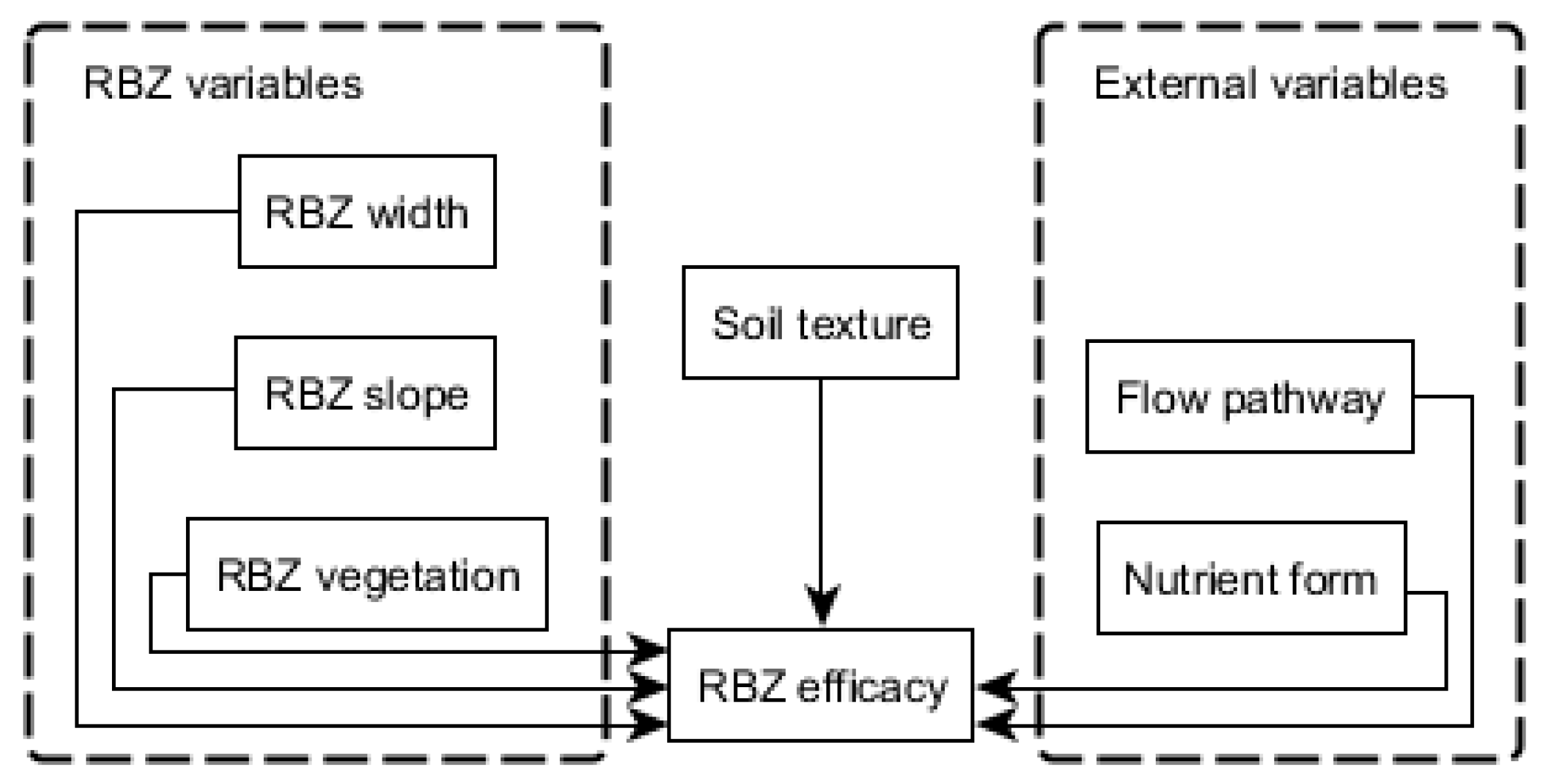
BN are directed acyclic graphs which link variables (called parent and child nodes) without feedback loops. The nodes and links of the BN were based on the literature listed above: the RBZ and external variables in the first column of Table 1 were considered as independent parent nodes directly influencing RBZ efficacy as the final child (output) node of the BN (Figure 2).
In a BN, discrete states have to be defined for each node. They have to be exhaustive and mutually exclusive. Apart from flow pathway, the states of the nominal variables were groups of the reported values (see columns three and four in Table 1). The original nutrient forms were aggregated to the three states “particulate”, “mixed”, and “dissolved” based on the preliminary regression analyses. The various values of soil texture were grouped into (i) the three states “fine” (clayey soils), “medium” (loamy and silty soils), and “coarse” (sandy soils), and (ii) only two states “fine” and “coarse” (comprising loamy, silty, and sandy soils). The plant species composition, structure, and management of RBZ varied widely in the literature and were simplified to “grass” (herbaceous) and “woody” (with shrubs and trees).
In contrast to the nominal variables, the three continuous variables had to be discretized. Different discretization approaches exist but seemingly no optimal one [59,60]. Given the uneven value distribution and to acknowledge the limited data availability for parent nodes, we used the common equal-frequency approach. For RBZ width, however, we slightly adjusted the quantiles to match legal regulations. Since one aim of this study was to assess the effect of state definition on model accuracy, different numbers of quantiles were used (see Table 1).
2.4. BN Training and Evaluation—Importance of Nodes and State Definition
BNs with different number of states were trained using efficacy values with data for all parent nodes (n = 580) and the Maximum Likelihood parameter estimation. The training filled the conditional probability tables (CPT) which describe the probability of each state of the child node considering all possible states of the parent nodes, based on Bayes’ theorem. The different state definitions of four nodes (see Table 1) resulted in 72 different BNs. A 10-fold cross-validation—i.e., 90% of the data used for training and 10% for validation—was repeated 10 times for each of these BNs to compare prediction (classification) errors [59,61], i.e., the share of wrongly predicted output states. Ten different probabilities and prediction errors were thus obtained for each BN, ranging from 0 (all predictions correct) to 1 (all predictions wrong).
In order to assess how the state definition (state number) of the parent and output nodes affected the model performance, we used the non-parametric Wilcoxon Signed Rank test to determine whether the prediction errors differed significantly for parent nodes with different numbers of states (p < 0.05).
We also compared the complete BNs with all parent nodes to simplified BNs where the least important nodes were removed. The node importance was evaluated in two ways. Firstly, we applied the non-parametric Kruskal–Wallis test to each parent node to assess whether the RBZ efficacy for at least one state significantly differs from the other states (p < 0.05). Following Moe et al. [62], we also performed a classification tree analysis for each of the 72 possible state combinations. For all parent nodes we compared their relative importance and their occurrence in the classification trees to a random binary variable. In the simplified BN, we did not consider nodes with an influence close to the random variable and with a low occurrence in the classification trees (≤33%). As the values of the random variable vary with each repetition, we averaged the outcomes of 10 analyses to avoid misclassifications. The cross-validation and state evaluation were repeated with the 72 simplified BNs. We discarded undefined output from validation data outside the training data.
2.5. Implementation
All statistical analyses were conducted with the software R [63]. For the training and cross-validation of the BNs we used the R package bnlearn [64], and rpart [65] for the classification tree analysis. To exemplarily show the influence of individual parent nodes on the output, we trained an “optimal” BN—based on the prediction errors and the CPT size—with the full dataset. For the node of interest, we determined the BN output for each possible state by setting its probability to 1 (“hard evidence”) while assuming an equal probability of all states of the other parent nodes (“soft evidence”). These calculations were conducted using the R package gRain [66].
3. Results
3.1. Aggregating the Nutrient Forms
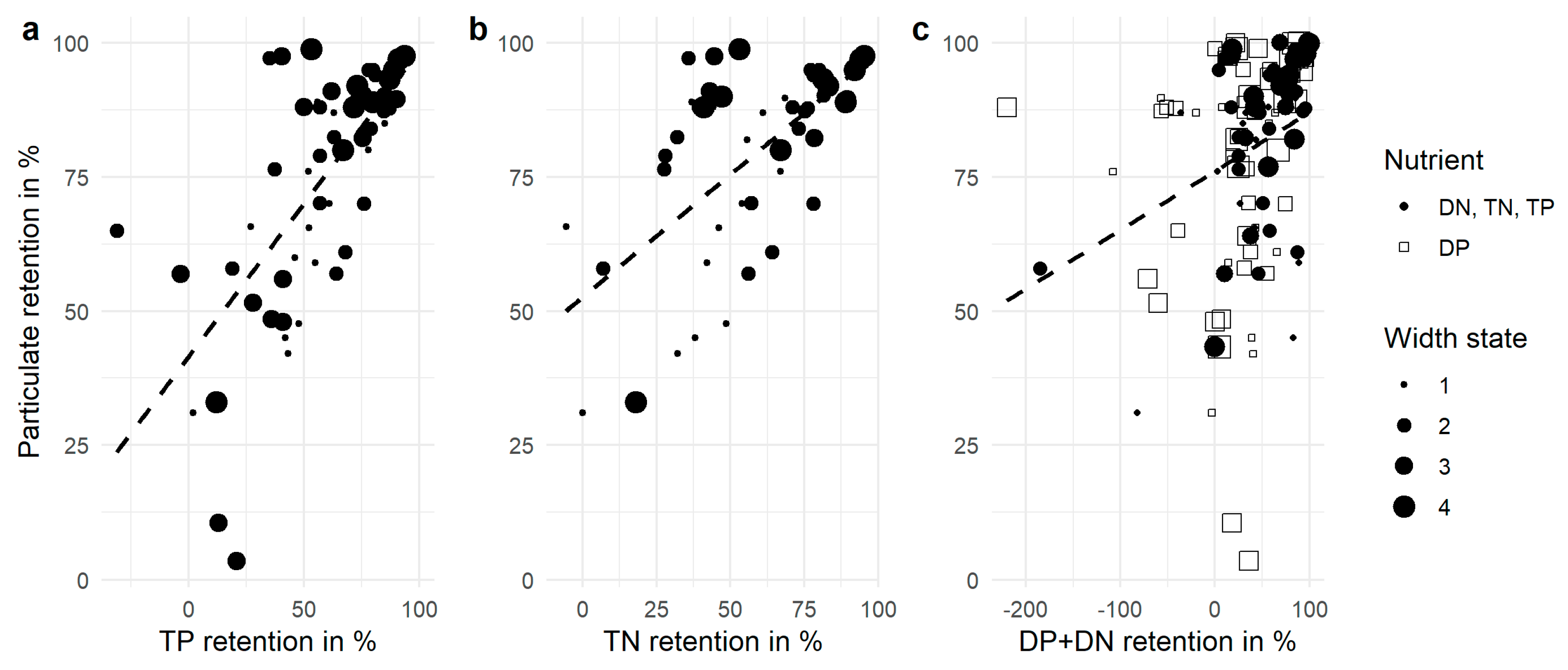
The retention of TN and TP were well correlated (r² = 0.64). Both were also more significantly correlated to sediment retention values (Figure 3, r² = 0.40–0.48, p < 0.0001) than the DN and DP retentions (r² = 0.09, p = 0.003). Based on these results, we considered TN and TP together as a separate “mixed” state of the node “nutrient form” and distinguished it from the “particulate” state (mainly sediment) and the “dissolved” nutrient forms, for which sedimentation is less important.
3.2. Variability of RBZ Efficacy and Importance of Nodes
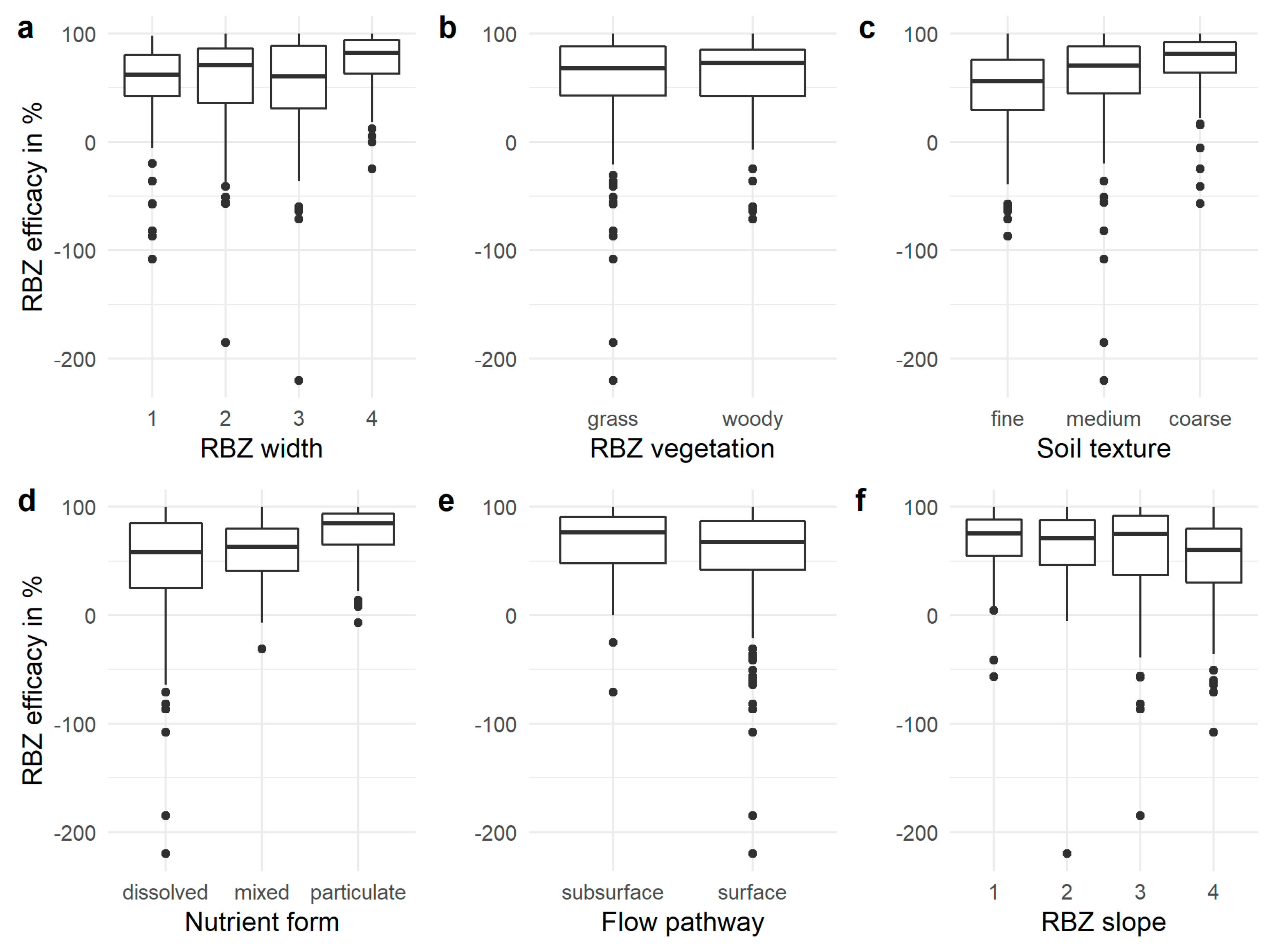
The reported RBZ efficacy ranged from complete retention to negative values, i.e., where the RBZ acted as sources. The distribution of all values was left-skewed with a median of 68% and a mode of 87%. This variability also resulted in a strong overlap between the states of the parent nodes (Figure 4). Therefore, even wide buffers can have a rather low efficacy (Figure 4a). However, the Kruskal–Wallis test revealed significant differences in RBZ efficacy among the states of all parent nodes (p ≤ 0.0003) except the flow pathway (p = 0.07) and RBZ vegetation (p = 0.8). For instance, RBZ are generally more effective with coarse soils than with fine and medium soils (Figure 4c) except for DP (not shown).
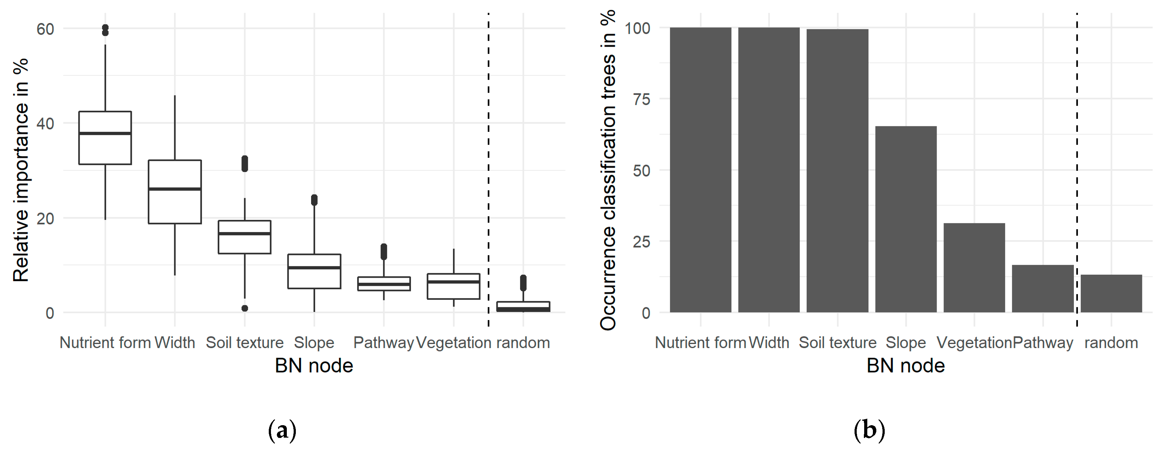
The classification tree analysis confirmed the strong influence of nutrient form, RBZ width, and soil texture on the RBZ efficacy (Figure 5). Despite its comparatively low importance (9%), RBZ slope occurred in 60% of the classification trees. The least important variables were RBZ vegetation and flow pathway (6%). Both variables rarely occurred in the trees, although they were more influential than a random variable (1.5%). This was especially the case for the flow pathway.
3.3. Cross-Validation and Evaluation of BNs
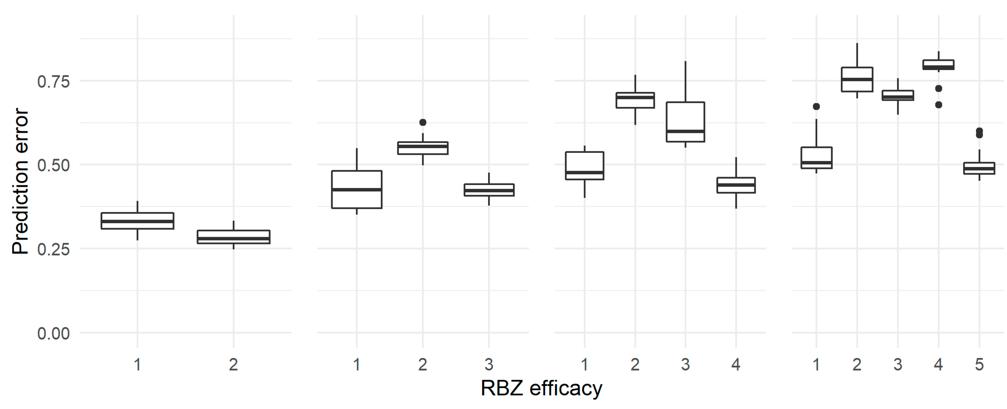
Fewer output states resulted in lower prediction errors, with average values over all BNs ranging from 0.31 (two states) to 0.66 (five states). However, the BNs predicted the lowest and highest output states significantly better than the intermediate states (Figure 6). These errors correspond to 62% of the expected error of a random predictor (E) for the two-state output (E = 0.5) up to 82% for the five-state output (E = 0.8). The values for the minimum and maximum states equaled on average 63% of E.
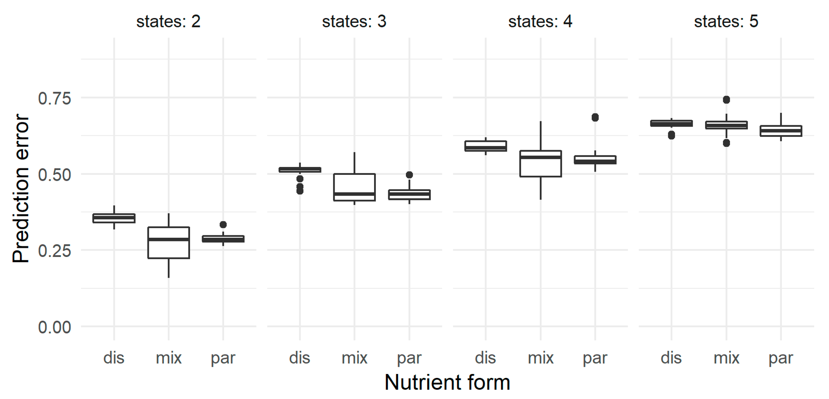
The prediction errors for RBZ efficacy were significantly lower when the nutrient form was “particulate” or “mixed” rather than “dissolved”, on average by 0.05 (−0.05–0.15, Figure 7). The impact of the flow pathway and the RBZ vegetation on the prediction error was negligible. The error even decreased on average by 0.01 after the BNs were simplified, i.e., by excluding the RBZ vegetation and the flow pathway. Limiting the database to the respective dominant state of these two nodes, i.e., to grassed RBZ and surface flow (n = 391), had no additional effect on the error.
The prediction errors were generally lowest when the parent nodes had three states (Table 3). However, for some BNs with all six parent nodes (“complete BN” in Table 3) choosing four states for the node “RBZ width” resulted in better predictions. Choosing two states, on the other hand, increased the predictions errors by up to 0.05 for RBZ width.
4. Discussion
4.1. BN Cross-Validation and Evaluation
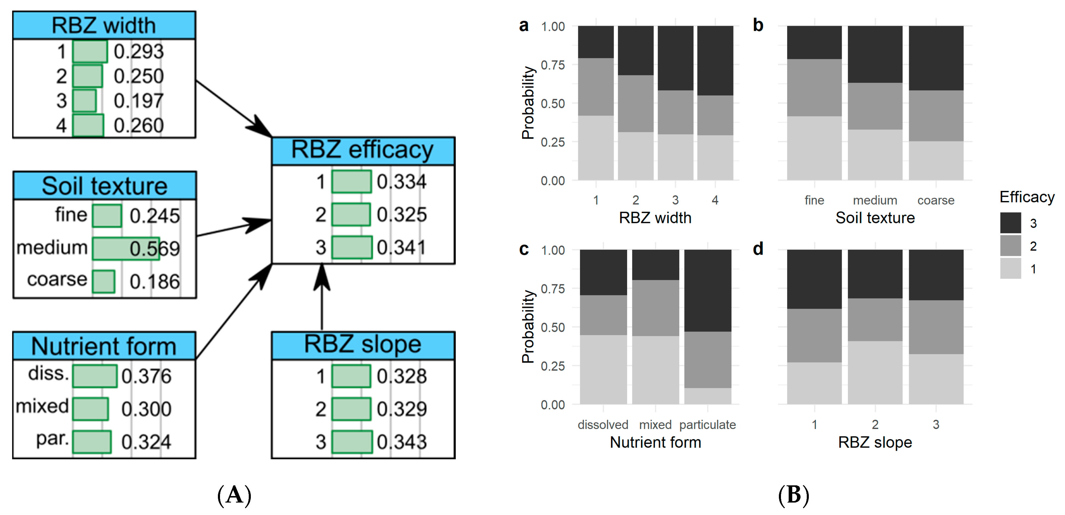
We tested the influence of nodes and states on RBZ efficacy in order to identify the minimum data requirement while ensuring no significant decrease in model performance and reliability. In this sense, the simplified BN with four out of the six considered parent nodes and with three (slope, soil texture) or four states (width) for the parent nodes as well as two to three output states can be considered as “optimal” among the tested alternatives (Figure 8A). The CPT size, i.e., the product of the state numbers, is 216 or 324 elements—which is manageable given the available input data [59]. Nonetheless, 0.3% or 0.9% of the predicted values during the cross-validation were undefined (compared to 0.2% for the smallest CPT size).
In accordance to the reviewed literature (cf. Methods), the BN reflects that a high RBZ efficacy was less probable for narrow than for broad RBZ (Figure 8B, a), for fine sediments than for coarse sediment (Figure 8B, b), and for dissolved nutrients than for particulate nutrients (Figure 8B, c). The more complex pattern for RBZ slope (Figure 8B, d) depended on the nutrient form (not shown). The higher probability of low RBZ efficacies for medium slopes occurred only for TN and TP. For particulate and dissolved nutrients, the efficacy of RBZ declined with increasing slope. Considering the dominance of studies on surface flow, this pattern can be explained by higher flow velocity and transport capacity on steeper slopes (cf. Methods). Nonetheless, it differs from findings of Zhang et al. [13], based on a smaller dataset, that sediment retention decreases with slopes steeper than 10% but increases with slopes below this threshold. At the plot scale—which dominates the collected data—flow resistance and other flow characteristics varies with slope gradient but also depends on the fragmentation of riparian vegetation [67] which is usually not available from RBZ studies. Following Zhang et al., more research on slope effects on RBZ efficacy is recommended to revise the inconsistent probabilities.
The use of these commonly available variables as nodes facilitates the envisaged application and validation of this first BN to estimate the retention efficacy of RBZ. This contributes to a better evaluation at medium to large scales of how RBZ can help to improve the water quality. The BN was significantly better in distinguishing effective (high state) from ineffective RBZ (low state) than between intermediate states (Figure 6). With two output states, the BN can for instance support or replace guidelines and design aids for effective RBZ based on single factors. For quantitative assessments, the discrete output states could be replaced by the average values of 45% and 90% efficacy in our database, or 30%, 70%, and 90% if a third state is needed. The high prediction errors hamper the use of more intermediate efficacy states at least in combination with our heterogeneous empirical dataset. Note that the BN is not intended to replace but rather complement other modelling approaches. For instance, Figure 8b illustrates that the BN can deal with uncertain evidence and provides probabilities of RBZ efficacy. Nonetheless, the high influence of RBZ width, soil texture, and slope emphasize the need of multivariate approaches in RBZ analyses.
Although the loss of information is a potential limitation of discrete BN [59], defining more than two states for parent nodes was only slightly helpful to improve the model accuracy. The prediction errors as well as the variability and the significant inconsistency among the reported efficacy values may indicate the need for supplementing BN nodes. Even with more input data than in previous studies, our analyses indicate that additional parent nodes are not necessarily useful to improve predictions if the data is biased and does not cover the variability of site conditions. For instance, the low influence of RBZ vegetation is in line with the similarity of woody and grassed RBZ as observed in previous studies (cf. Methods). However, the dominant grassed RBZ were on average narrower (9 m) than the woody RBZ (22.6 m). Moreover, the common distinction between grassed and woody RBZ does not consider the influence of different plant groups and species on the nutrient retention in RBZ [68,69]. Vegetation and root density seem to be promising to refine the state definition and to improve model predictions (cf. Methods), but such data is unavailable in existing RBZ studies.
4.2. Further BN Development
The current BN can be improved in different ways. The collection of training and validation data could be limited to specific experimental designs, scales, or site conditions. This simple approach would minimize the impact of some factors not explicitly considered in the BN at the expense of restricting our intended applicability at large scales. More nodes and states, on the other hand, require enough representative training data to fill the rapidly growing CPT. Expert knowledge can reduce the data demand (e.g., [70]) but its validation can be challenging [71]. We exemplarily discuss below constraints of the available data regarding the design and application of the BN (and other empirical models).
Firstly, only less than 20% of the datasets were on subsurface flow. The underrepresentation was most striking for DP (n = 10). Although limiting the dataset to surface flow did not reduce the prediction errors, the observed low influence of the flow pathway on RBZ efficacy and the (slightly) higher errors for dissolved nutrients (Figure 7) should be scrutinized with more (DP) data. However, revising the role of flow pathway may also require considering the contrasting effects of external factors like redox conditions on the retention of P (oxidation/reduction of iron oxides) and N (denitrification) either as separate node or as additional DN and DP states of the nutrient node.
Secondly, the current BN may overestimate the efficacy of “real-world” RBZ because most literature values were measured in rather short-term studies. However, aging buffer strips may turn from sinks to sources [34,53,72] and foster eutrophication if poorly maintained [72,73,74]. Negative values occurred in 26 datasets and comprised mostly DP (n = 16) and DN (n = 9), followed by TN (n = 3), TP (n = 2), and PP (n = 1). Given the variety of underlying processes and the small number of cases, they could not be considered as a separate state in the output node. Apart from the remobilization of P from saturated RBZ soils as DP [34,45], P-rich colluvium in RBZ can be remobilized during heavy rainfall or flood events. Detailed maps on water-soluble P, degree of P saturation, and residual soil P in agricultural areas (e.g., [7]) might be helpful to overcome this limitation in future BN. The data availability is, however, more challenging for other processes such as the decay of plants [74,75].
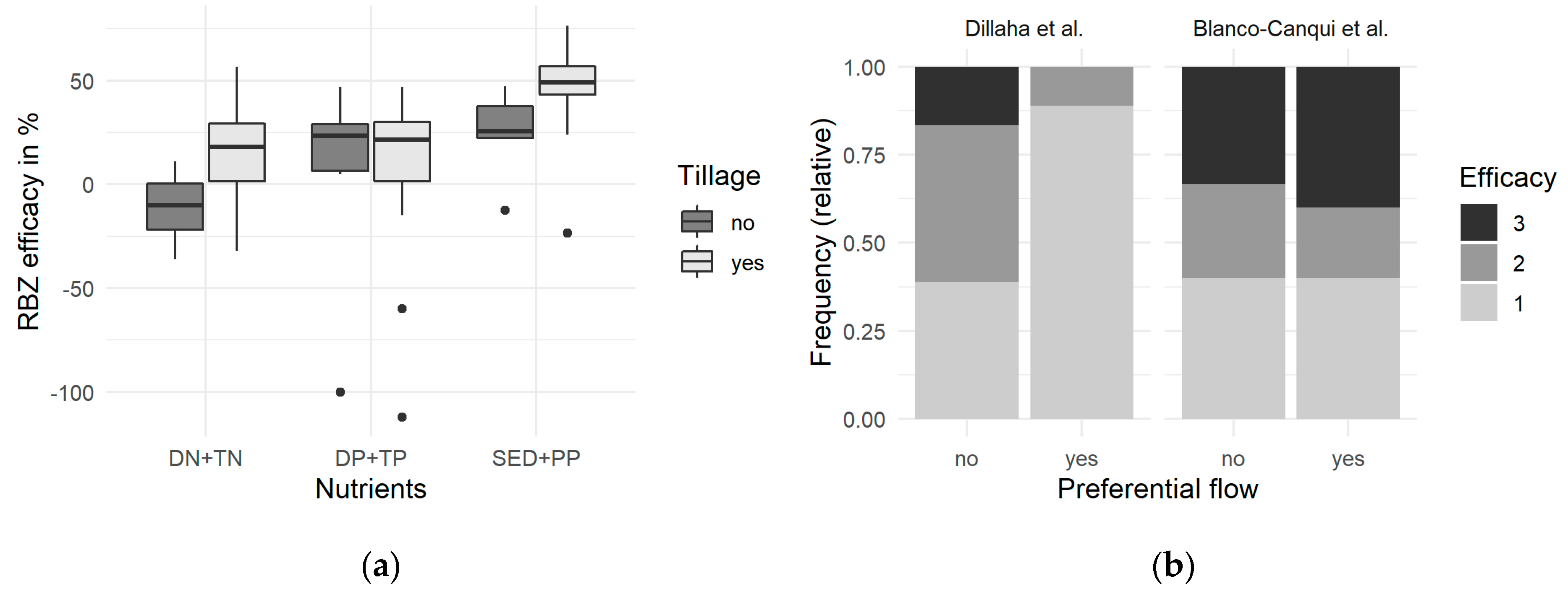
Thirdly, other below-average retention efficacies e.g., for sediment retention in our data collection were explained by conservation tillage (CT) [76,77] and preferential flow [78] in the catchment of RBZ. CT, i.e., minimum- and no-till, has increasingly been used worldwide during the last decade [79], and might do so in the future [80], to reduce sediment and PP losses from agricultural land. However, the accumulation of labile P pools in top soils and the development of preferential flow paths belowground can unintendedly impair the RBZ efficacy to retain soluble, immediately bioavailable P [34,81]. No-till can also increase the water and nitrate flux entering RBZ from adjacent fields [82]. While more water flux can reduce the nitrate retention in subsurface flow [46], higher (initial) concentrations favor its retention [47].
In the few available quantitative studies on CT, no-till reduced significantly the RBZ efficacy compared to conventional till, notably except for P (Figure 9a). However, most of the values already belonged to the lowest efficacy state (RBZ efficacy < 55%). Therefore, the influence of CT on the BN output would currently be rather low. It might also not be representative for other output states. By separating the soil texture in RBZ and their catchments, the BN could consider some of the complex impacts of CT together with nutrient form.
As a side effect, these two BN nodes can generally integrate the effects of hydrology [46,87], land use, and land management [16,21]. These variables affect the concentration [47,88], timing, amount, and composition of nutrient and sediment entering RBZ and have been used in other empirical RBZ models (e.g., [16,46]).
Fourthly, most published RBZ studies were plot studies which are typically constructed with uniform slopes to favor sheet-flow conditions under which RBZ work best [48,89]. However, they neglect the tendency of water to converge and develop preferential flow paths at larger scales and within natural terrain [90,91,92]. According to the very few available quantitative studies, preferential flow can reduce the efficiency of RBZ [78,85,86,93] (Figure 9b, left). Nonetheless, RBZ may perform equally well depending on RBZ width and structure as well as the runoff conditions [86,91] (Figure 9b, right). According to our data collection, plot studies reported on average less effective RBZ than field- and watershed studies which can be explained by the narrower RBZ in these plot studies. Therefore, more field studies are needed to reliably quantify how preferential flow affects the efficacy of RBZ.
In an extended BN, the current output state could be reduced based on the probability of preferential flow. The likelihood of preferential surface flow is often estimated from digital elevation models by applying area thresholds or variants thereof [94] or from linear anthropogenic features [95]. Similar slope–area relationships are known for e.g., the topographic index [96,97] and soil erosion [98] which also influence the variability and composition of nutrients.
5. Conclusions
The discrete, multivariate BNs to predict RBZ efficacy developed and evaluated in our study are flexible tools which e.g., provide probabilities instead of exact outcomes. They predict sufficiently well the RBZ efficacies collected from previous studies. The “optimal” BNs have four parent nodes (width, slope, nutrient form, and soil texture) with more than two states and up to three states for RBZ efficacy. The resulting CPTs are manageable with the available input data. RBZ vegetation and flow pathway are found to be not relevant.
The model performance is better for the highest and lowest states of RBZ efficacy compared to the intermediate states. The BNs could thus complement or replace existing design guidelines for RBZ. The expected limitations for more detailed predictions arise from missing data for other variables as discussed in the literature as well as the heterogeneous database which does not adequately represent all site conditions. This is relevant for the vegetation type which typical states “grass” and “woody” comprise different species. Additionally, most data are obtained from plot-scale studies which typically do not consider preferential flow. More field-scale studies are needed to better represent preferential flow in BNs. Future research should focus on the database to better cover the different state combinations and to provide new data to train and validate the relationships.
Supplementary Materials
The following are available online at https://www.mdpi.com/2073-4441/12/3/617/s1, Table S1: Data table, File S2: BN in Figure 8a as Hugin. net file.
Author Contributions
Conceptualization, A.G. and M.V.; methodology, A.G. and M.V.; software, A.G.; validation, A.G.; formal analysis, A.G.; investigation, A.G., P.F., and M.V.; resources, A.G. and P.F.; data curation, A.G. and M.V.; writing—original draft preparation, A.G.; writing—review and editing, A.G., H.H.N., P.F., J.K., and M.V.; visualization, A.G.; supervision, M.V.; project administration, J.K. and M.V.; funding acquisition, J.K. and M.V. All authors have read and agreed to the published version of the manuscript.
Funding
This research was funded by the German “Bundesministerium für Bildung und Forschung (Federal Ministry of Education and Research)”, grant number 01LC1618A within the 2015–2016 BiodivERsA COFUND call. Peter Fischer was financed by the “Ministerium für Umwelt, Klima und Energiewirtschaft (Ministry of the Environment, Climate Protection and the Energy Sector) Baden-Württemberg” within the project “Retention of sediments, nutrients, and pesticides in riparian buffer zones”.
Acknowledgments
We thank Daniela Pietras (University of Rennes) for assisting the data collection. We are thankful to three anonymous reviewers for their detailed and valuable comments.
Conflicts of Interest
The authors declare no conflict of interest. The funders had no role in the design of the study; in the collection, analyses, or interpretation of data; in the writing of the manuscript, or in the decision to publish the results.
References
- Le Moal, M.; Gascuel-Odoux, C.; Ménesguen, A.; Souchon, Y.; Étrillard, C.; Levain, A.; Moatar, F.; Pannard, A.; Souchu, P.; Lefebvre, A.; et al. Eutrophication: A new wine in an old bottle? Sci. Total Environ. 2019, 651, 1–11. [Google Scholar] [CrossRef] [PubMed] [Green Version]
- Evans, A.E.V.; Mateo-Sagasta, J.; Qadir, M.; Boelee, E.; Ippolito, A. Agricultural water pollution: Key knowledge gaps and research needs. Curr. Opin. Environ. Sust. 2019, 36, 20–27. [Google Scholar] [CrossRef]
- FAO; IMWI. More People, More Food, Worse Water? A Global Review of Water Pollution from Agriculture; Mateo-Sagasta, J., Marjani Zadeh, S., Turral, H., Eds.; FAO: Rome, Italy; IMWI: Colombo, Sri Lanka, 2018; p. 207. [Google Scholar]
- Diamantini, E.; Lutz, S.R.; Mallucci, S.; Majone, B.; Merz, R.; Bellin, A. Driver detection of water quality trends in three large European river basins. Sci. Total Environ. 2018, 612, 49–62. [Google Scholar] [CrossRef] [PubMed]
- Schwarzenbach, R.P.; Egli, T.; Hofstetter, T.B.; von Gunten, U.; Wehrli, B. Global Water Pollution and Human Health. Annu. Rev. Environ. Resour. 2010, 35, 109–136. [Google Scholar] [CrossRef]
- Withers, P.J.A.; Neal, C.; Jarvie, H.P.; Doody, D.G. Agriculture and Eutrophication: Where Do We Go from Here? Sustainability 2014, 6, 5853. [Google Scholar] [CrossRef] [Green Version]
- Fischer, P.; Pöthig, R.; Venohr, M. The degree of phosphorus saturation of agricultural soils in Germany: Current and future risk of diffuse P loss and implications for soil P management in Europe. Sci. Total Environ. 2017, 599, 1130–1139. [Google Scholar] [CrossRef] [PubMed]
- European Environment Agency. European Waters: Assessment of Status and Pressures 2018; Publications Office of the European Union: Luxembourg, Luxembourg, 2018; p. 85. [Google Scholar]
- Stutter, M.I.; Chardon, W.J.; Kronvang, B. Riparian Buffer Strips as a Multifunctional Management Tool in Agricultural Landscapes: Introduction. J. Environ. Qual. 2012, 41, 297–303. [Google Scholar] [CrossRef] [Green Version]
- Feld, C.K.; Fernandes, M.R.; Ferreira, M.T.; Hering, D.; Ormerod, S.J.; Venohr, M.; Gutiérrez-Cánovas, C. Evaluating riparian solutions to multiple stressor problems in river ecosystems-A conceptual study. Water Res. 2018, 139, 381–394. [Google Scholar] [CrossRef]
- Mander, Ü.; Tournebize, J.; Tonderski, K.; Verhoeven, J.T.A.; Mitsch, W.J. Planning and establishment principles for constructed wetlands and riparian buffer zones in agricultural catchments. Ecol. Eng. 2017, 103, 296–300. [Google Scholar] [CrossRef]
- Dorioz, J.-M.; Wang, D.; Poulenard, J.; Trevisan, D. The effect of grass buffer strips on phosphorus dynamics—A critical review and synthesis as a basis for application in agricultural landscapes in France. Agric. Ecosyst. Environ. 2006, 117, 4–21. [Google Scholar] [CrossRef]
- Zhang, X.; Liu, X.; Zhang, M.; Dahlgren, R.A.; Eitzel, M. A review of vegetated buffers and a meta-analysis of their mitigation efficacy in reducing nonpoint source pollution. J. Environ. Qual. 2010, 39, 76–84. [Google Scholar] [CrossRef] [PubMed]
- Muñoz-Carpena, R.; Parsons, J.E.; Gilliam, J.W. Modeling hydrology and sediment transport in vegetative filter strips. J. Hydrol. 1999, 214, 111–129. [Google Scholar] [CrossRef]
- Lowrance, R.; Altier, L.S.; Williams, R.G.; Inamdar, S.P.; Sheridan, J.M.; Bosch, D.D.; Hubbard, R.K.; Thomas, D.L. REMM: The Riparian Ecosystem Management Model. J. Soil Water Conserv. 2000, 55, 27–34. [Google Scholar]
- Hassanzadeh, Y.T.; Vidon, P.G.; Gold, A.J.; Pradhanang, S.M.; Addy Lowder, K. RZ-TRADEOFF: A New Model to Estimate Riparian Water and Air Quality Functions. Water 2019, 11, 769. [Google Scholar] [CrossRef] [Green Version]
- Weissteiner, C.J.; Bouraoui, F.; Aloe, A. Reduction of nitrogen and phosphorus loads to European rivers by riparian buffer zones. Knowl. Manag. Aquat. Ecosyst. 2013, 408, 15. [Google Scholar] [CrossRef]
- Hook, P.B. Sediment retention in rangeland riparian buffers. J. Environ. Qual. 2003, 32, 1130–1137. [Google Scholar] [CrossRef]
- Lee, P.; Smyth, C.; Boutin, S. Quantitative review of riparian buffer width guidelines from Canada and the United States. J. Environ. Manag. 2004, 70, 165–180. [Google Scholar] [CrossRef]
- Broadmeadow, S.; Nisbet, T.R. The effects of riparian forest management on the freshwater environment: A literature review of best management practice. HESS 2004, 8, 286–305. [Google Scholar] [CrossRef]
- Dosskey, M.G.; Helmers, M.J.; Eisenhauer, D.E. A design aid for determining width of filter strips. J. Soil Water Conserv. 2008, 63, 232–241. [Google Scholar] [CrossRef]
- Gumiere, S.J.; Le Bissonnais, Y.; Raclot, D.; Cheviron, B. Vegetated filter effects on sedimentological connectivity of agricultural catchments in erosion modelling: A review. ESPL 2011, 36, 3–19. [Google Scholar] [CrossRef]
- Liu, X.; Zhang, X.; Zhang, M. Major factors influencing the efficacy of vegetated buffers on sediment trapping: A review and analysis. J. Environ. Qual. 2008, 37, 1667–1674. [Google Scholar] [CrossRef] [PubMed]
- Yuan, Y.; Bingner, R.L.; Locke, M.A. A review of effectiveness of vegetative buffers on sediment trapping in agricultural areas. Ecohydrology 2009, 2, 321–336. [Google Scholar] [CrossRef]
- Mayer, P.M.; Reynolds, S.K.; McCutchen, M.D.; Canfield, T.J. Meta-analysis of nitrogen removal in riparian buffers. J. Environ. Qual. 2007, 36, 1172–1180. [Google Scholar] [CrossRef] [PubMed]
- Barton, D.N.; Kuikka, S.; Varis, O.; Uusitalo, L.; Henriksen, H.J.; Borsuk, M.; de la Hera, A.; Farmani, R.; Johnson, S.; Linnell, J.D. Bayesian networks in environmental and resource management. Integr. Environ. Assess. Manag. 2012, 8, 418–429. [Google Scholar] [CrossRef]
- Borsuk, M.E.; Stow, C.A.; Reckhow, K.H. A Bayesian network of eutrophication models for synthesis, prediction, and uncertainty analysis. Ecol. Model. 2004, 173, 219–239. [Google Scholar] [CrossRef]
- Kelly, R.A.; Jakeman, A.J.; Barreteau, O.; Borsuk, M.E.; ElSawah, S.; Hamilton, S.H.; Henriksen, H.J.; Kuikka, S.; Maier, H.R.; Rizzoli, A.E.; et al. Selecting among five common modelling approaches for integrated environmental assessment and management. Environ. Model. Softw. 2013, 47, 159–181. [Google Scholar] [CrossRef]
- Marcot, B.G.; Penman, T.D. Advances in Bayesian network modelling: Integration of modelling technologies. Environ. Model. Softw. 2019, 111, 386–393. [Google Scholar] [CrossRef]
- Phan, T.D.; Smart, J.C.R.; Capon, S.J.; Hadwen, W.L.; Sahin, O. Applications of Bayesian belief networks in water resource management: A systematic review. Environ. Model. Softw. 2016, 85, 98–111. [Google Scholar] [CrossRef]
- McVittie, A.; Norton, L.; Martin-Ortega, J.; Siameti, I.; Glenk, K.; Aalders, I. Operationalizing an ecosystem services-based approach using Bayesian Belief Networks: An application to riparian buffer strips. Ecol. Econ. 2015, 110, 15–27. [Google Scholar] [CrossRef] [Green Version]
- Castelle, A.J.; Johnson, A.W.; Conolly, C. Wetland and stream buffer size requirements-a review. J. Environ. Qual. 1994, 23, 878–882. [Google Scholar] [CrossRef] [Green Version]
- Collins, A.L.; Hughes, G.; Zhang, Y.; Whitehead, J. Mitigating diffuse water pollution from agriculture: Riparian buffer strip performance with width. CAB Rev. Perspect. Agric. Veter. Sci. Nutr. Nat. Resour. 2009, 4, 15. [Google Scholar] [CrossRef]
- Dodd, R.J.; Sharpley, A.N. Conservation practice effectiveness and adoption: Unintended consequences and implications for sustainable phosphorus management. Nutr. Cycl. Agroecosyst. 2016, 104, 373–392. [Google Scholar] [CrossRef]
- Dosskey, M.G. Toward quantifying water pollution abatement in response to installing buffers on crop land. Environ. Manag. 2001, 28, 577–598. [Google Scholar] [CrossRef] [PubMed]
- Dosskey, M.G.; Vidon, P.; Gurwick, N.P.; Allan, C.J.; Duval, T.P.; Lowrance, R. The Role of Riparian Vegetation in Protecting and Improving Chemical Water Quality in Streams. JAWRA 2010, 46, 261–277. [Google Scholar] [CrossRef]
- Hickey, M.B.C.; Doran, B. A review of the efficiency of buffer strips for the maintenance and enhancement of riparian ecosystems. Water Qual. Res. J. Can. 2004, 39, 311–317. [Google Scholar] [CrossRef]
- Hill, A.R. Nitrate removal in stream riparian zones. J. Environ. Qual. 1996, 25, 743–755. [Google Scholar] [CrossRef]
- Hill, A.R. Groundwater nitrate removal in riparian buffer zones: A review of research progress in the past 20 years. Biogeochemistry 2019, 143, 347–369. [Google Scholar] [CrossRef]
- Hoffmann, C.C.; Kjaergaard, C.; Uusi-Kämppä, J.; Hansen, H.C.B.; Kronvang, B. Phosphorus retention in riparian buffers: Review of their efficiency. J. Environ. Qual. 2009, 38, 1942–1955. [Google Scholar] [CrossRef]
- Krutz, L.J.; Senseman, S.A.; Zablotowicz, R.M.; Matocha, M.A. Reducing herbicide runoff from agricultural fields with vegetative filter strips: A review. Weed Sci. 2005, 53, 353–367. [Google Scholar] [CrossRef]
- Lacas, J.-G.; Voltz, M.; Gouy, V.; Carluer, N.; Gril, J.-J. Using grassed strips to limit pesticide transfer to surface water: A review. Agron. Sustain. Dev. 2005, 25, 253–266. [Google Scholar] [CrossRef] [Green Version]
- Mayer, P.M.; Reynolds, S.K., Jr.; Canfield, T.J. Riparian Buffer Width, Vegetative Cover, and Nitrogen Removal Effectiveness; EPA/600/R-05/118; U.S. Environmental Protection Agency: Washington, DC, USA, 2005; p. 27. [Google Scholar]
- Polyakov, V.; Fares, A.; Ryder, M.H. Precision riparian buffers for the control of nonpoint source pollutant loading into surface water: A review. Environ. Rev. 2005, 13, 129–144. [Google Scholar] [CrossRef]
- Roberts, W.M.; Stutter, M.I.; Haygarth, P.M. Phosphorus retention and remobilization in vegetated buffer strips: A review. J. Environ. Qual. 2012, 41, 389–399. [Google Scholar] [CrossRef] [PubMed]
- Sweeney, B.W.; Newbold, J.D. Streamside Forest Buffer Width Needed to Protect Stream Water Quality, Habitat, and Organisms: A Literature Review. JAWRA 2014, 50, 560–584. [Google Scholar] [CrossRef]
- Valkama, E.; Usva, K.; Saarinen, M.; Uusi-Kämppä, J. A Meta-Analysis on Nitrogen Retention by Buffer Zones. J. Environ. Qual. 2018. [Google Scholar] [CrossRef] [Green Version]
- Wenger, S. A Review of the Scientific Literature on Riparian Buffer Width, Extent and Vegetation; Office of Public Service and Outreach, Institute of Ecology: Athens, GA, USA, 1999; p. 59. [Google Scholar]
- Borin, M.; Vianello, M.; Morari, F.; Zanin, G. Effectiveness of buffer strips in removing pollutants in runoff from a cultivated field in North-East Italy. Agric. Ecosyst. Environ. 2005, 105, 101–114. [Google Scholar] [CrossRef]
- Fiener, P.; Auerswald, K. Effectiveness of grassed waterways in reducing runoff and sediment delivery from agricultural watersheds. J. Environ. Qual. 2003, 32, 927–936. [Google Scholar] [CrossRef] [PubMed]
- Pärn, J.; Pinay, G.; Mander, Ü. Indicators of nutrients transport from agricultural catchments under temperate climate: A review. Ecol. Indic. 2012, 22, 4–15. [Google Scholar] [CrossRef]
- King, S.E.; Osmond, D.L.; Smith, J.; Burchell, M.R.; Dukes, M.; Evans, R.O.; Knies, S.; Kunickis, S. Effects of Riparian Buffer Vegetation and Width: A 12-Year Longitudinal Study. J. Environ. Qual. 2016, 45, 1243–1251. [Google Scholar] [CrossRef] [Green Version]
- Osborne, L.L.; Kovacic, D.A. Riparian vegetated buffer strips in water-quality restoration and stream management. Freshw. Biol. 1993, 29, 243–258. [Google Scholar] [CrossRef]
- Yang, F.; Yang, Y.; Li, H.; Cao, M. Removal efficiencies of vegetation-specific filter strips on nonpoint source pollutants. Ecol. Eng. 2015, 82, 145–158. [Google Scholar] [CrossRef]
- Schauder, H.; Auerswald, K. Long-term trapping efficiency of a vegetated filter strip under agricultural use. J. Plant Nutr. Soil Sci. 1992, 155, 489–492. [Google Scholar] [CrossRef]
- Vidon, P.; Hill, A.R. Denitrification and patterns of electron donors and acceptors in eight riparian zones with contrasting hydrogeology. Biogeochemistry 2004, 71, 259–283. [Google Scholar] [CrossRef]
- Barling, R.D.; Moore, I.D. Role of buffer strips in management of waterway pollution: A review. Environ. Manag. 1994, 18, 543–558. [Google Scholar] [CrossRef]
- Darch, T.; Carswell, A.; Blackwell, M.S.A.; Hawkins, J.M.B.; Haygarth, P.M.; Chadwick, D. Dissolved Phosphorus Retention in Buffer Strips: Influence of Slope and Soil Type. J. Environ. Qual. 2015, 44, 1216–1224. [Google Scholar] [CrossRef] [PubMed] [Green Version]
- Chen, S.H.; Pollino, C.A. Good practice in Bayesian network modelling. Environ. Model. Softw. 2012, 37, 134–145. [Google Scholar] [CrossRef]
- Nojavan, A.F.; Qian, S.S.; Stow, C.A. Comparative analysis of discretization methods in Bayesian networks. Environ. Model. Softw. 2017, 87, 64–71. [Google Scholar] [CrossRef]
- Marcot, B.G. Metrics for evaluating performance and uncertainty of Bayesian network models. Ecol. Model. 2012, 230, 50–62. [Google Scholar] [CrossRef]
- Moe, S.J.; Haande, S.; Couture, R.-M. Climate change, cyanobacteria blooms and ecological status of lakes: A Bayesian network approach. Ecol. Model. 2016, 337, 330–347. [Google Scholar] [CrossRef] [Green Version]
- Team, R.C. R: A Language and Environment for Statistical Computing; R Foundation for Statistical Computing: Vienna, Austria, 2017. [Google Scholar]
- Scutari, M. Learning Bayesian Networks with the bnlearn R Package. J. Stat. Softw. 2010, 35, 1–22. [Google Scholar] [CrossRef] [Green Version]
- Therneau, T.; Atkinson, B.; Ripley, B. rpart: Recursive Partitioning and Regression Trees. 1–11 April 2017. Available online: https://cran.r-project.org/web/packages/rpart/index.html (accessed on 14 June 2019).
- Højsgaard, S. Graphical Independence Networks with the gRain Package for R. J. Stat. Softw. 2012, 1. [Google Scholar] [CrossRef] [Green Version]
- Zhao, Q.; Zhang, Y.; Xu, S.; Ji, X.; Wang, S.; Ding, S. Relationships between Riparian Vegetation Pattern and the Hydraulic Characteristics of Upslope Runoff. Sustainability 2019, 11. [Google Scholar] [CrossRef] [Green Version]
- Kelly, J.M.; Kovar, J.L.; Sokolowsky, R.; Moorman, T.B. Phosphorus uptake during four years by different vegetative cover types in a riparian buffer. Nutr. Cycl. Agroecosyst. 2007, 78, 239–251. [Google Scholar] [CrossRef]
- Missaoui, A.M.; Boerma, H.R.; Bouton, J.H. Genetic variation and heritability of phosphorus uptake in Alamo switchgrass grown in high phosphorus soils. Field Crops Res. 2005, 93, 186–198. [Google Scholar] [CrossRef]
- Oniśko, A.; Druzdzel, M.J.; Wasyluk, H. Learning Bayesian network parameters from small data sets: Application of Noisy-OR gates. Int. J. Approx. Reason. 2001, 27, 165–182. [Google Scholar] [CrossRef] [Green Version]
- Pitchforth, J.; Mengersen, K. A proposed validation framework for expert elicited Bayesian Networks. Expert Syst. Appl. 2013, 40, 162–167. [Google Scholar] [CrossRef] [Green Version]
- Cooper, J.R.; Gilliam, J.W. Phosphorus redistribution from cultivated fields into riparian areas. Soil Sci. Soc. Am. J. 1987, 51, 1600–1604. [Google Scholar] [CrossRef]
- Stutter, M.I.; Langan, S.J.; Lumsdon, D.G. Vegetated buffer strips can lead to increased release of phosphorus to waters: A biogeochemical assessment of the mechanisms. Environ. Sci. Technol. 2009, 43, 1858–1863. [Google Scholar] [CrossRef]
- Uusi-Kämppä, J.; Jauhiainen, L. Long-term monitoring of buffer zone efficiency under different cultivation techniques in boreal conditions. Agric. Ecosyst. Environ. 2010, 137, 75–85. [Google Scholar] [CrossRef]
- Uusi-Kämppä, J. Phosphorus purification in buffer zones in cold climates. Ecol. Eng. 2005, 24, 491–502. [Google Scholar] [CrossRef]
- Shipitalo, M.J.; Bonta, J.V.; Dayton, E.A.; Owens, L.B. Impact of Grassed Waterways and Compost Filter Socks on the Quality of Surface Runoff from Corn Fields. J. Environ. Qual. 2010, 39, 1009–1018. [Google Scholar] [CrossRef] [Green Version]
- Newbold, J.D.; Herbert, S.; Sweeney, B.W.; Kiry, P.; Alberts, S.J. Water Quality Functions of a 15-Year-Old Riparian Forest Buffer System. JAWRA 2010, 46, 299–310. [Google Scholar] [CrossRef]
- Dillaha, T.A.; Sherrard, J.H.; Lee, D.; Mostaghimi, S.; Shanholtz, V.O. Evaluation of vegetative filter strips as a best management practice for feed lots. J. Water Pollut. Control Fed. 1988, 60, 1231–1238. [Google Scholar]
- Kassam, A.; Friedrich, T.; Derpsch, R. Global spread of Conservation Agriculture. Int. J. Environ. Stud. 2019, 76, 29–51. [Google Scholar] [CrossRef]
- Prestele, R.; Hirsch, A.L.; Davin, E.L.; Seneviratne, S.I.; Verburg, P.H. A spatially explicit representation of conservation agriculture for application in global change studies. Glob. Chang. Biol. 2018, 24, 4038–4053. [Google Scholar] [CrossRef] [PubMed]
- Jarvie, H.P.; Johnson, L.T.; Sharpley, A.N.; Smith, D.R.; Baker, D.B.; Bruulsema, T.W.; Confesor, R. Increased Soluble Phosphorus Loads to Lake Erie: Unintended Consequences of Conservation Practices? J. Environ. Qual. 2017, 46, 123–132. [Google Scholar] [CrossRef] [PubMed] [Green Version]
- Daryanto, S.; Wang, L.; Jacinthe, P.-A. Impacts of no-tillage management on nitrate loss from corn, soybean and wheat cultivation: A meta-analysis. Sci. Rep. 2017, 7, 12117. [Google Scholar] [CrossRef]
- Eghball, B.; Gilley, J.E.; Kramer, L.A.; Moorman, T.B. Narrow grass hedge effects on phosphorus and nitrogen in runoff following manure and fertilizer application. J. Soil Water Conserv. 2000, 55, 172–176. [Google Scholar]
- Raffaelle, J.B., Jr.; McGregor, K.C.; Foster, G.R.; Cullum, R.F. Effect of narrow grass strips on conservation reserve land converted to cropland. Trans. ASAE 1997, 40, 1581–1587. [Google Scholar] [CrossRef]
- Dillaha, T.A.; Sherrard, J.H.; Lee, D.; Shanholtz, V.O.; Mostaghimi, S.; Magette, W.L. Use of Vegetative Filter Strips to Minimize Sediment and Phosphorus Losses from Feedlots; Phase 1, Experimental Plot Studies; Virginia Polytechnic Institute and State University Blacksburg: Blacksburg, VA, USA, 1986; p. 68. [Google Scholar]
- Blanco-Canqui, H.; Gantzer, C.J.; Anderson, S.H. Performance of grass barriers and filter strips under interrill and concentrated flow. J. Environ. Qual. 2006, 35, 1969–1974. [Google Scholar] [CrossRef]
- White, M.J.; Arnold, J.G. Development of a simplistic vegetative filter strip model for sediment and nutrient retention at the field scale. Hydrol. Process. 2009, 23, 1602–1616. [Google Scholar] [CrossRef] [Green Version]
- Vidon, P.G.F.; Hill, A.R. Landscape controls on nitrate removal in stream riparian zones. WRR 2004, 40. [Google Scholar] [CrossRef] [Green Version]
- Habibiandehkordi, R.; Lobb, D.A.; Sheppard, S.C.; Flaten, D.N.; Owens, P.N. Uncertainties in vegetated buffer strip function in controlling phosphorus export from agricultural land in the Canadian prairies. Environ. Sci. Pollut. Res. 2017, 24, 18372–18382. [Google Scholar] [CrossRef] [PubMed]
- Verstraeten, G.; Poesen, J.; Gillijns, K.; Govers, G. The use of riparian vegetated filter strips to reduce river sediment loads: An overestimated control measure? Hydrol. Process. 2006, 20, 4259–4267. [Google Scholar] [CrossRef]
- Helmers, M.J.; Eisenhauer, D.E.; Dosskey, M.G.; Franti, T.G.; Brothers, J.M.; McCullough, M.C. Flow pathways and sediment trapping in a field-scale vegetative filter. Trans. ASAE 2005, 48, 955–968. [Google Scholar] [CrossRef]
- Dosskey, M.G.; Helmers, M.J.; Eisenhauer, D.E.; Franti, T.G.; Hoagland, K.D. Assessment of concentrated flow through riparian buffers. J. Soil Water Conserv. 2002, 57, 336–343. [Google Scholar]
- Daniels, R.B.; Gilliam, J.W. Sediment and chemical load reduction by grass and riparian filters. Soil Sci. Soc. Am. J. 1996, 60, 246–251. [Google Scholar] [CrossRef]
- Yadav, B.; Hatfield, K. Stream network conflation with topographic DEMs. Environ. Model. Softw. 2018, 102, 241–249. [Google Scholar] [CrossRef]
- Hösl, R.; Strauss, P.; Glade, T. Man-made linear flow paths at catchment scale: Identification, factors and consequences for the efficiency of vegetated filter strips. Landsc. Urban Plan. 2012, 104, 245–252. [Google Scholar] [CrossRef]
- Beven, K.J.; Kirkby, M.J. A physically based, variable contributing area model of basin hydrology. Hydrol. Sci. B 1979, 24, 43–69. [Google Scholar] [CrossRef] [Green Version]
- Beven, K. TOPMODEL: A critique. Hydrol. Process. 1997, 11, 1069–1085. [Google Scholar] [CrossRef]
- De Vente, J.; Poesen, J.; Arabkhedri, M.; Verstraeten, G. The sediment delivery problem revisited. Prog. Phys. Geogr. 2007, 31, 155–178. [Google Scholar] [CrossRef] [Green Version]
Figure 1.
Overview of collected data; (a) complete/incomplete datasets per country (n = 341, cf. Table 2), (b) number of studies per publication year (n = 139).
Figure 1.
Overview of collected data; (a) complete/incomplete datasets per country (n = 341, cf. Table 2), (b) number of studies per publication year (n = 139).

Figure 2.
BN structure with nodes and links. We assumed that the reported soil textures are similar in the RBZ and their catchments.
Figure 2.
BN structure with nodes and links. We assumed that the reported soil textures are similar in the RBZ and their catchments.

Figure 3.
RBZ efficacy to retain total phosphorus (TP) (a), total nitrogen (TN) (b), as well as dissolved N and P (DP, DN) (c) compared to particulates as collected from the literature with (dashed) lines of best fit. Higher state numbers correspond to broader RBZ.
Figure 3.
RBZ efficacy to retain total phosphorus (TP) (a), total nitrogen (TN) (b), as well as dissolved N and P (DP, DN) (c) compared to particulates as collected from the literature with (dashed) lines of best fit. Higher state numbers correspond to broader RBZ.

Figure 4.
RBZ efficacy for the states of the parent nodes using the maximum number of states as given in Table 1. Higher state numbers correspond to broader RBZ (a) and steeper RBZ (f).
Figure 4.
RBZ efficacy for the states of the parent nodes using the maximum number of states as given in Table 1. Higher state numbers correspond to broader RBZ (a) and steeper RBZ (f).

Figure 5.
Relative importance (a) and occurrence of BN nodes (b) in the classification trees compared to a random binary variable. Note the changed order of (RBZ) vegetation and (flow) pathway.
Figure 5.
Relative importance (a) and occurrence of BN nodes (b) in the classification trees compared to a random binary variable. Note the changed order of (RBZ) vegetation and (flow) pathway.

Figure 6.
Cross-validation results for the different output states based on the 72 complete BNs with all nodes. Higher state numbers correspond to more effective RBZ.
Figure 6.
Cross-validation results for the different output states based on the 72 complete BNs with all nodes. Higher state numbers correspond to more effective RBZ.

Figure 7.
Cross-validation results for disaggregated (dis), particulate (par), and mixed (total, mix) nutrients and different numbers of output states.
Figure 7.
Cross-validation results for disaggregated (dis), particulate (par), and mixed (total, mix) nutrients and different numbers of output states.

Figure 8.
The “optimal” BN with three output states (A) influence diagram (Supplementary File S2, par. = particulate, diss. = dissolved), (B) probability of the output states (RBZ efficacy) given hard evidence of the parent node mentioned below the subfigures a–d (state with probability = 1 on x axes) and soft evidence (here equal probability of all states) of the other parent nodes. Higher state numbers correspond to broader RBZ (RBZ width), steeper RBZ (RBZ slope), and more efficient RBZ.

Figure 9.
Examples of non-representative and inconsistent effects on RBZ efficacy, (a) tillage (data from references [74,76,83,84], paired n = 30), (b) preferential flow (left: data from references [78,85], right: data from [86], without switchgrass barrier, paired n = 6).


Table 1.
List of riparian buffer zones (RBZ) and external variables used as nodes in the Bayesian networks (BN) and their discrete states. State definitions are shown as comma-separated lists. The variables (nodes) RBZ width, soil texture, RBZ slope, and RBZ efficacy were discretized using different numbers of states (given in separate lines, cf. section on BN design for details on the state definition).
| Variable (Node) | Unit | States | Definition | Data per State |
|---|---|---|---|---|
| RBZ width | m | 1, 2 | <10, 10–220 | 315, 265 |
| 1, 2, 3 | <5.1, <10.1, 10.1–220 | 170, 214, 196 | ||
| 1, 2, 3, 4 | <5.1, <10, <15, 15–220 | 170, 145, 114, 151 | ||
| RBZ vegetation | - | Grass | Including e.g., giant cane | 433 |
| Woody | With shrubs and trees | 147 | ||
| Soil texture | - | Fine, medium, coarse | Clayey (fL, CL, SiC, C, SC), silty-loamy (L, SiL, Si, SCL), sandy (SL, cL, S, SSi, LS) 1 | 142, 330, 108 |
| Fine, coarse | Clayey, silty to sandy | 142, 408 | ||
| Nutrient form | - | Particulate | Particulate P (PP), sediment | 188 (17 + 171) |
| Mixed | Total P (TP) and N (TN) | 174 (95 + 79) | ||
| Dissolved | Dissolved P (DP) 2 and N (DN) 3 | 218 (87 + 131) | ||
| Flow pathway | - | Surface | Surface runoff | 480 |
| Subsurface | (Including) groundwater | 100 | ||
| RBZ slope | % | 1, 2 | <5, 5–22 | 262, 318 |
| 1, 2, 3 | <3.1, <7.5, 7.5–22 | 190, 191, 199 | ||
| 1, 2, 3, 4 | <3, <5, <10, 10–22 | 124, 138, 157, 161 | ||
| RBZ efficacy | % | 1, 2 | <68.3, ≥68.3 | 290, 290 |
| 1, 2, 3 | <55, <82.3, ≥82.3 | 193, 193, 194 | ||
| 1, 2, 3, 4 | <42.6, <68.3, <87.5, ≥87.5 | 145, 145, 145, 145 | ||
| 1, 2, 3, 4, 5 | <35.5, <60.6, <78.5, <89.8, ≥89.8 | 116, 116, 115, 117, 116 |
1 Loam (L), clay (C), sand (S), silt (Si), fine (f), coarse (c), 2 including orthophosphate, 3 i.e., nitrate.
Table 2.
Completeness of literature values.
| Value | Complete (Count) | Incomplete (Count) |
|---|---|---|
| Studies 1 | 104 | 36 |
| Datasets | 269 | 72 |
| Efficacy values | 580 | 98 |
| Countries 2 | 13 | 12 |
| Variables (nodes) | All | Slope, soil texture |
1 One study with partly incomplete soil data, 2 three countries without complete data.
Table 3.
Effect of the state number of parent nodes on prediction errors for different BNs. Mean errors and p values based on the outcomes of six BNs (RBZ width, RBZ slope) and nine BNs (soil texture). The nodes “flow pathway” and “RBZ vegetation” in complete BNs have only two states and are not shown.
| BN | RBZ Efficacy | Node | Mean Prediction Error | Significance (p Value) 1 | |||
|---|---|---|---|---|---|---|---|
| Number of States | Two States | Three States | Four States | 2 < 3 2 | 3 < 4 | ||
| Complete | 2 | RBZ slope | 0.32 | 0.26 | 0.31 | 0.031* | 0.984 |
| 3 | 0.51 | 0.45 | 0.46 | 0.016* | 0.656 | ||
| 4 | 0.59 | 0.55 | 0.56 | 0.016* | 0.844 | ||
| 5 | 0.67 | 0.65 | 0.64 | 0.016* | 0.109 | ||
| 2 | RBZ width | 0.32 | 0.31 | 0.30 | 0.031* | 0.031* | |
| 3 | 0.47 | 0.47 | 0.47 | 0.719 | 0.109 | ||
| 4 | 0.59 | 0.55 | 0.55 | 0.016* | 0.922 | ||
| 5 | 0.67 | 0.66 | 0.64 | 0.281 | 0.016* | ||
| 2 | Soil texture | 0.32 | 0.30 | - | 0.002** | - | |
| 3 | 0.48 | 0.47 | - | 0.010** | - | ||
| 4 | 0.58 | 0.55 | - | 0.002** | - | ||
| 5 | 0.66 | 0.65 | - | 0.002** | - | ||
| Simplified | 2 | RBZ slope | 0.30 | 0.30 | 0.30 | 0.219 | 0.984 |
| 3 | 0.48 | 0.46 | 0.48 | 0.016* | 1 | ||
| 4 | 0.55 | 0.54 | 0.56 | 0.500 | 1 | ||
| 5 | 0.64 | 0.64 | 0.64 | 0.578 | 0.844 | ||
| 2 | RBZ width | 0.30 | 0.30 | 0.30 | 0.047* | 0.781 | |
| 3 | 0.48 | 0.47 | 0.47 | 0.047* | 0.953 | ||
| 4 | 0.58 | 0.53 | 0.54 | 0.016* | 0.844 | ||
| 5 | 0.64 | 0.64 | 0.64 | 0.656 | 0.219 | ||
| 2 | Soil texture | 0.30 | 0.30 | - | 0.963 | - | |
| 3 | 0.47 | 0.48 | - | 0.898 | - | ||
| 4 | 0.55 | 0.55 | - | 0.980 | - | ||
| 5 | 0.64 | 0.64 | - | 0.590 | - | ||
1 One-sided Mann–Whitney U test, symbols: p < 0.001 (***), < 0.01 (**), < 0.05 (*), 2 prediction error smaller with two states than with three states.
© 2020 by the authors. Licensee MDPI, Basel, Switzerland. This article is an open access article distributed under the terms and conditions of the Creative Commons Attribution (CC BY) license (http://creativecommons.org/licenses/by/4.0/).
Share and Cite
MDPI and ACS Style
Gericke, A.; Nguyen, H.H.; Fischer, P.; Kail, J.; Venohr, M. Deriving a Bayesian Network to Assess the Retention Efficacy of Riparian Buffer Zones. Water 2020, 12, 617. https://doi.org/10.3390/w12030617
AMA Style
Gericke A, Nguyen HH, Fischer P, Kail J, Venohr M. Deriving a Bayesian Network to Assess the Retention Efficacy of Riparian Buffer Zones. Water. 2020; 12(3):617. https://doi.org/10.3390/w12030617
Chicago/Turabian StyleGericke, Andreas, Hong Hanh Nguyen, Peter Fischer, Jochem Kail, and Markus Venohr. 2020. "Deriving a Bayesian Network to Assess the Retention Efficacy of Riparian Buffer Zones" Water 12, no. 3: 617. https://doi.org/10.3390/w12030617
Note that from the first issue of 2016, this journal uses article numbers instead of page numbers. See further details here.