Feasibility of the Use of Variable Speed Drives in Center Pivot Systems Installed in Plots with Variable Topography

Abstract

Pumping systems are the largest energy consumers in center pivot irrigation systems. One action to reduce energy consumption is to adjust the pumping pressure to that which is strictly needed by using variable speed drives (VSDs). The objective of this study was to determine the feasibility of including VSDs in pumping systems that feed center pivot systems operating in an area with variable topography. The VSPM (Variable Speed Pivot Model) was developed to perform hydraulic and energy analyses of center pivot systems using the EPANET hydraulics engine. This tool is able to determine the elevation of each tower for each position of the center pivot using any type of digital elevation model. It is also capable of simulating, in an accurate manner, the performance of the center pivot controlled with a VSD. The tool was applied to a real case study, located in Albacete, Spain. The results show a reduction in energy consumption of 12.2%, with specific energy consumptions of 0.214 and 0.244 kWh m⁻³ of distributed water obtained for the variable speed and fixed speed of the pumping station, respectively. The results also show that for an irrigation season, to meet the water requirements of the maize crop in the region of the study (627 mm), an average annual savings of 14,107.35 kWh was obtained, which resulted in an economic savings of 2821.47€.

1. Introduction

The quantity and quality of food needed to satisfy all the demands of the population will become a major concern worldwide in the following years. It is expected that by the year 2050, there will be a world population of 9.15 billion people [1]. The increase of food production to satisfy demand is a challenge for agricultural professionals, who require the use of techniques focused on increasing production efficiency. Increasing use efficiency in food production requires the use of improved technology in all production processes, as well as improving the efficiency of irrigation systems. Irrigated agriculture accounts for 16% of the world’s cultivated area and is expected to produce 44% of world food by 2050 [1,2,3].

Sustainable use of water resources could be accomplished increasing the efficiency of irrigation systems, thereby reducing the amount of water and energy to satisfy crop water requirements. In this regard, technological developments in the infrastructures of irrigation systems contribute to increasing water use efficiency. However, this efficiency increase is related to a significant increase in energy consumption in recent years [4].

According to [5], sprinkler irrigation systems represent around 11% (35 million hectares) of the total irrigated areas in the world. Within this method, the most outstanding systems are conventional sprinklers, traveling guns, center pivots, and linear-moving laterals. With eight million hectares of irrigated area, the center pivot system represents 23% of the area irrigated by sprinkler irrigation systems.

Center pivot irrigation consists of the application of water through a moving lateral line with several water outlets supported on moving towers, which revolve around a fixed pivot point (center tower) and irrigate a circular area [6,7]. This equipment is considered a highly efficient system compared to other irrigation systems. It is flexible and easily operable, which reduces labor and maintenance costs. It can also be operated on surfaces with variable topography, resulting in conservation of water, energy, and time [8]. However, the initial cost of the equipment and the required energy demands at the pumping station are some of its main limitations.

The reduction of the energy consumption of pumping stations that feed irrigation systems has been studied by several researchers. Pumping stations are the largest consumers of energy in pressurized irrigation systems, especially in situations where underground water resources are used.

Gilley et al. [9] suggested several changes in center pivot systems: switching high and medium pressure sprinklers to low pressure emitters, changing nozzle size and spacing, or changing irrigation intervals and maintenance to increase pumping station efficiency. Moreno et al. [10] developed a new methodology to obtain the characteristic curves of the pump, thereby minimizing the costs of the pumping station. In a later study, Moreno et al. [11] stated that the energy consumption of the center pivot, which irrigates an area of 75 ha, can be minimized by adopting measures like increasing the lateral line’s diameter, reducing the equipment’s operating time, and increasing the flow per unit of area. Barbosa et al. [12] concluded that constant center pivot monitoring is essential to maintaining adequate energy efficiency levels when assessing the behavior of different energy efficiency indicators for a center pivot operating in variable topography.

In center pivot equipment, the pumping station is designed to meet the most critical situation, i.e., the position of the lateral line where there is the highest elevation point and the greatest need for higher pumping pressure [13]. However, this situation is variable along with the lateral line rotation in the irrigated area due to topographic differences. This means that the pumping station is oversized during most of the lateral line rotation, and the energy is wasted. Pressure regulating valves are installed before the emitters, so pressure fluctuations that are due to topographical differences and oversizing of the pumping station do not influence the flow rate of the emitters [14].

An option to adjust the pumping pressure of this equipment is the use of variable speed drives (VSDs) to control the speed of these pumps [15,16]. This control provides a substantial reduction in power in relation to the reduction of flow and pressure in pressurized irrigation systems [13,17].

Several researchers have used variable speed drives to control pumping stations to reduce energy consumption. Hanson et al. [18], in a center pivot system with a well pumping unit, concluded that variable speed pumps save about 32% of the energy. Lamaddalena et al. [19] showed that 27% to 35% of energy savings can be achieved using VSD in two Italian irrigation districts operating with three parallel horizontal axis pumps. Brar et al. [20] concluded that a 9.6% energy reduction is possible for a 13.6 m difference in the irrigated area for a study containing 100 center pivots in Nebraska (USA), with each pivot containing a pumping station. In this study, digital elevation models (DEMs) with a spatial resolution of 10 m × 10 m were used to obtain the topographic characteristics of the irrigated areas.

King et al. [13] stated that the optimum efficiency in terms of energy and water use can be achieved when the pumping station is able to maintain the required minimum pressure regardless of the operating conditions. Scaloppi et al. [21] stated that the point of minimum pressure is constantly moving along the lateral line because it is influenced by the topography of the irrigated area. They also presented theoretical bases for the calculation of this movement.

However, working with the minimum pressure does not always guarantee the lowest power consumption due to variations in the operating point of the pump and variable performance when working at low frequencies [17,22]. In addition, most of these studies did not take into account the effect of the VSD efficiency on the final result. Therefore, it is important to consider VSD efficiency in energy savings accounting and not assume that this efficiency will always be constant and high [17].

In a study on VSD efficiency, King et al. [13] reported that a pumping station with a VSD can save 15.8% and 20.2% of its energy compared to fixed speed pumping (for uniform and variable rate irrigation, respectively) without considering the inefficiency of the VSD. When the efficiency of the VSD is accounted for, there are 7.5% and 12.4% energy savings, respectively.

The main novelty of the present study is developing a simulation model of hydraulic behavior by considering the hydraulic elements of the irrigation system in detail and integrating the energy characteristics of the pumping station and topographic characteristics through digital elevation models (DEMs). In this way, energy efficient technologies and management strategies can be developed to reduce energy use to ensure sustainable irrigation without reductions in the efficiency of water application.

The objective of the present study was to determine the feasibility of including variable speed drives in pumping systems that feed center pivot irrigation systems operating in areas with variable topography. Considering this objective, the VSPM (Variable Speed Pivot Model) tool was developed, in which the hydraulic simulation model of the pivot was integrated into a simulation model of the pumping station so that, with data related to topography, flow rate, and pressure, the power supply could be adjusted to the actual demand of the system. In addition, it is useful to determine the potential of reduction from the perspective of the energy, economics, and sustainability of the installation of the VSDs in these irrigation systems.

2. Material and Methods

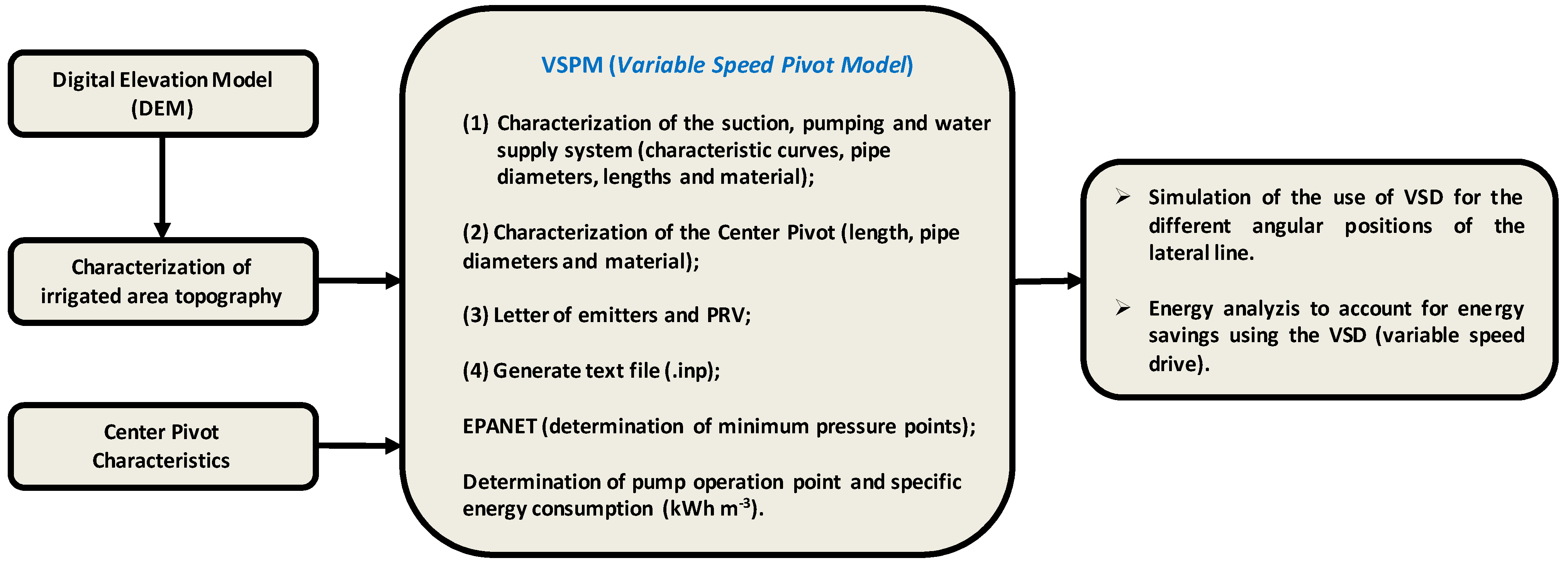
2.1. Proposed Procedure

The proposed methodology has the following steps, as presented in 1. For the development of this model and data acquisition, a real center pivot was used. However, this model can be used for pivots of different sizes and with different numbers of towers.

The characterization of the irrigated area, along with the characteristics of the pumping station and irrigation system from the manufacturers’ technical data, were inserted into the VSPM (Variable Speed Pivot Model) tool to process and edit the input data. Subsequently, the hydraulic simulation was calculated using the EPANET hydraulic engine. The hydraulic simulation results were then used to determine the energy consumption of the irrigation system under study.

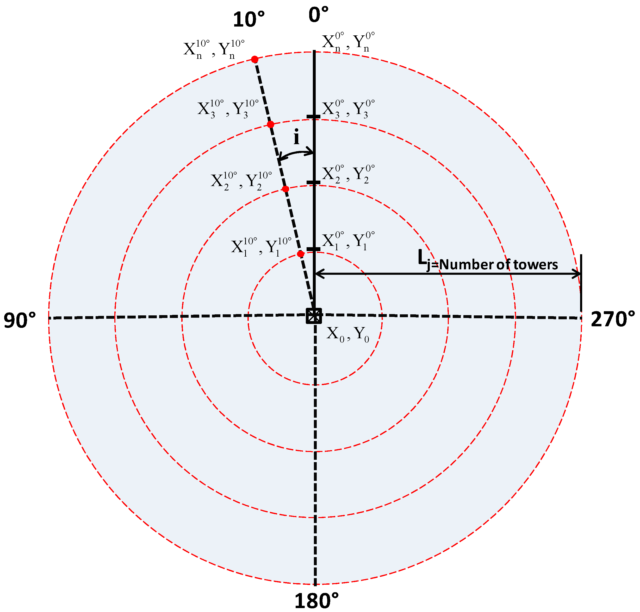
2.2. Topography of the Irrigated Area

As shown in Figure 1, the elevation values of the moving towers were obtained through Digital Elevation Models (DEMs) (with a spatial resolution of 5 m × 5 m), which were freely obtained from the PNOA (Spanish National Program of aerial photogrammetry). These products are freely available for any location in Spain. The developed tool is able to use any type of DEM.

The utilized DEMs (.tif formatted images) were loaded into the QGIS^® Desktop 3.2.1 software (QGIS Development Team, Open Source Geospatial Foundation). In this software, the geographical coordinates (X, Y) of the point referring to the center of the pivot (X₀, Y₀) were defined.

To obtain the X and Y coordinates of all moving towers in different angular positions relative to the center pivot’s lateral line, a computational routine was developed in the MATLAB^® 2018b software. Automatically, with the values of the geographic coordinates and the distance between towers, the elevation values were determined for 36 angular positions of the lateral line, equally spaced by 10°, with the North position of the lateral line as the position of angle 0°, as in Figure 2.

The calculation of the geographical coordinates X, Y of each moving tower (j) was carried out as follows:

$${\mathrm{X}}_{\mathrm{j}}^{\mathrm{i}}={\mathrm{X}}_0+{\mathrm{L}}_{\mathrm{j}}·\cos (\mathrm{i}),\mathrm{with}1\le \mathrm{j}\le \mathrm{Number}\mathrm{of}\mathrm{towers}$$

(1)

$${\mathrm{Y}}_{\mathrm{j}}^{\mathrm{i}}={\mathrm{Y}}_0+{\mathrm{L}}_{\mathrm{j}}·\sin (\mathrm{i}),\mathrm{with}1\le \mathrm{j}\le \mathrm{Number}\mathrm{of}\mathrm{towers}$$

(2)

where i is the angular position of the lateral line (0°, 10°, …, 350°), j is the number of moving towers, in this case, 1 ≤ j < ≤ 9, and L_j is the distance from the center tower to the index tower j, m.

Thus, for the center pivot under study, the dimensions of the nine moving towers were obtained in 36 different angular positions of the lateral line, resulting in 324 elevation values.

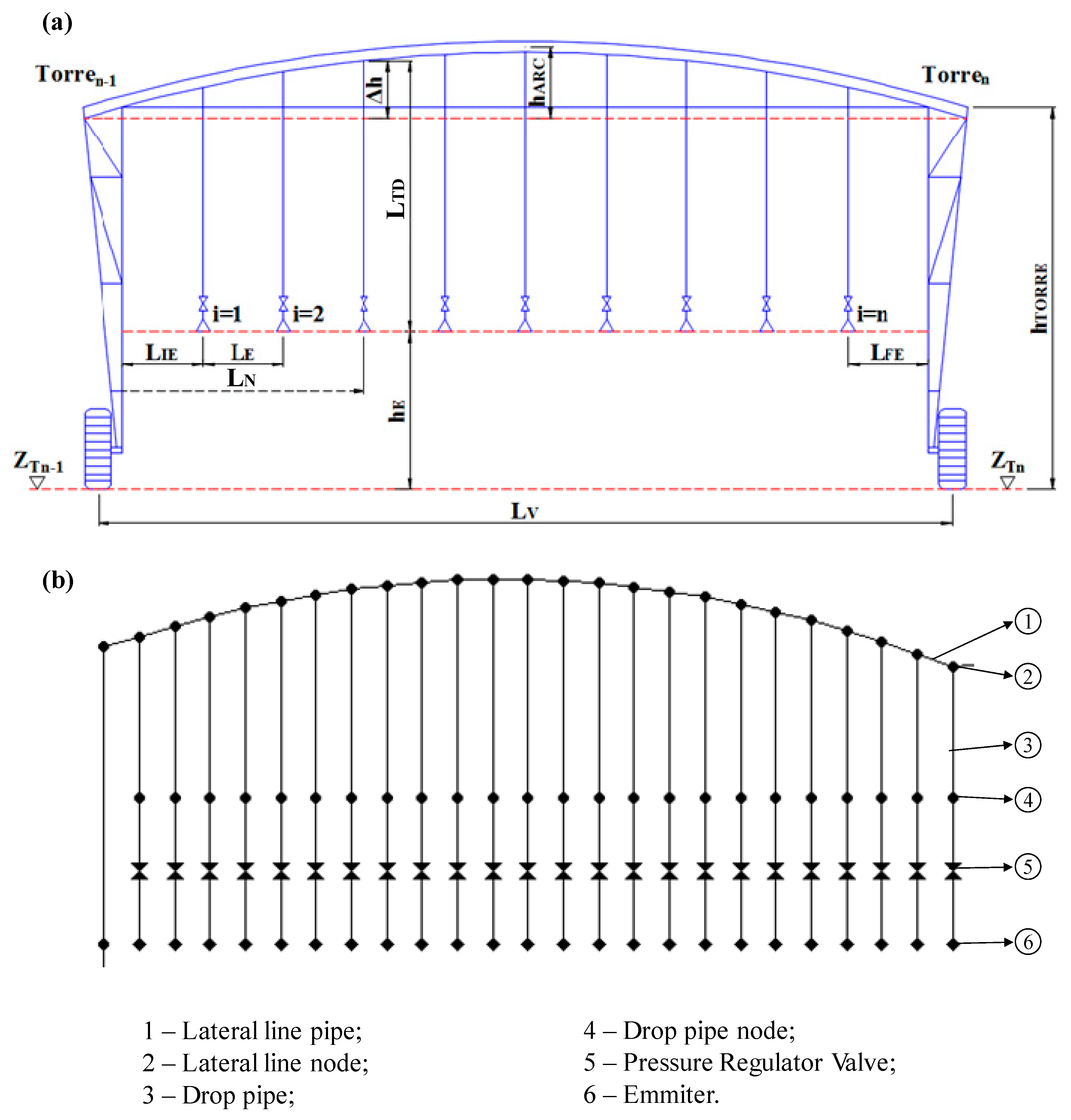
2.3. Hydraulic Model Description

The simulation of the operation of the center pivot irrigation system, for different angular positions of the lateral line of the center pivot, was carried out using EPANET software [23]. With this aim, the VSPM tool was developed. The function of this tool is to edit the input data required by the EPANET software in addition to energy analysis, as shown in Figure 1.

Center pivot irrigation system simulations, for different lateral line angular positions, was carried out using EPANET software [23]. With this aim, the VSPM tool was developed. The function of this tool is to edit the input data required by the EPANET software in addition to energy analysis, as shown in Figure 1. Figure 3a shows the dimensions of the lateral line span and Figure 3b shows the EPANET network map of the first span of the center pivot lateral line.

The VSPM tool has four steps: (1) characterization of the suction, pumping, and water supply systems, (2) characterization of the center pivot, (3) emitters and pressure regulating valves (PRV), (4) generation of the text file in the EPANET format.

The system that includes suction, pumping, and water supply was pre-determined containing the following hydraulic elements: a fixed level reservoir (water source), a pumping station, and a supply pipe composed of three different links. The required information for these components are: elevation of the water level in the reservoir, elevation of the ground where the pumping station is located, length, pipe diameter and roughness coefficient (depending on the selected head loss equation) of all links, and the pairs of values (Q-H) constituting the pump characteristic curve, as taken from the manufacturer’s technical data.

In the center pivot characterization module, the center pivot’s equipment information is inserted: the elevation of the pivot point and the elevation of the moving towers, as well as pipe lengths, pipe diameters, and the roughness coefficient of the pivot point, lateral line, and drop pipes.

In the module related to emitters and pressure regulating valves (PRVs), the emission coefficients of the emitters and the working pressure of the PRVs are inserted. If information about the emitter’s distribution on the pivot is not available, it remains possible to generate and simulate a commonly used commercial emitter distribution with this tool.

Finally, the VSPM tool generates a text file (in .inp format) with all the hydraulic model information entered by the user. This file consists of input data, which is required by EPANET to perform the hydraulic simulation. In the VSPM modules, the flow rate and discharge coefficient of each emitter, the node elevations, and the pipe lengths were determined.

2.3.1. Flow Rate of the Emitters

The total flow of the irrigation system is the sum of the flow rate of each emitter along the lateral line. The flow rate of the emitters (in m³ h⁻¹) was calculated according to the area corresponding to each water outlet, and the gross depth to be applied to the rotation time was specified by the manufacturer, as proposed by Valiantzas et al. [24]. The flow rate for the first outlet of each span (Equation (3)) and the remainder of each outlet (Equation (4)) was calculated. The lengths used are shown in Figure 3a:

$${\mathrm{q}}_{\mathrm{x}=1}=\frac{2\pi {\mathrm{L}}_{\mathrm{I}\mathrm{E}}^2}{1000}\frac{\mathrm{L}\mathrm{b}}{\mathrm{T}\mathrm{g}},\mathrm{for}\mathrm{x}=1$$

(3)

$${\mathrm{q}}_{\mathrm{x}}=\frac{2\pi {\mathrm{R}}_{\mathrm{inst}}{\mathrm{L}}_{\mathrm{E}}}{1000}\frac{\mathrm{L}\mathrm{b}}{\mathrm{T}\mathrm{g}},\mathrm{for}2\le \mathrm{x}\le \mathrm{n}$$

(4)

where q_x is the flow rate of the outlet with order number x (1 ≤ x ≤ n), m³ h⁻¹, L_IE is spacing between the tower and the first emitter (x = 1), m, L_E is the spacing between the emitters with order number x (2 ≤ x ≤ n), m, R_inst is the radius of the installation of the emitter, relative to the center tower, m, Lb is the gross irrigation depth (9 mm), and Tg is the rotation time (21 h).

After the acquisition of the flow rate values at each water outlet (q_x), the discharge coefficient (k_e, Equation (5)) of each emitter was determined. The value of the pressure in the emitter was the same as the value of the PRV nominal pressure (H_prv), assuming an ideal valve:

$${\mathrm{k}}_{\mathrm{e}}=\frac{{\mathrm{q}}_{\mathrm{i}}}{{\mathrm{H}}_{\mathrm{p}\mathrm{r}\mathrm{v}}^{\mathsf{\beta }}}$$

(5)

where k_e is emitter discharge coefficient, m^2.5 h⁻¹, H_prv is the PRV nominal pressure, m, and β is the pressure exponent, in this case with a value of 0.5.

2.3.2. Determination of Elevations and Lengths

The spans lengths (Equation (6)) and the water outlet relative distance to the previous moving tower (Equation (7)) were calculated:

$${\mathrm{L}}_{\mathrm{S}}{=\mathrm{L}}_{\mathrm{IE}}{+\mathrm{L}}_{\mathrm{FE}}+\left[\left({\mathrm{N}}_{\mathrm{O}}-1\right){\mathrm{L}}_{\mathrm{E}}\right]$$

(6)

$${\mathrm{L}}_{\mathrm{N}}=\{\begin{array}{l}\mathrm{N}=1\Rightarrow {\mathrm{R}}_{\mathrm{T}}+{\mathrm{L}}_{\mathrm{IE}}\\ 2\le \mathrm{N}<\mathrm{n}\Rightarrow {\mathrm{L}}_{\mathrm{N}=1}+{\mathrm{L}}_{\mathrm{E}}\\ \mathrm{N}=\mathrm{n}\Rightarrow {\mathrm{L}}_{2\le \mathrm{N}<\mathrm{n}}+{\mathrm{L}}_{\mathrm{F}\mathrm{E}}\end{array}$$

(7)

where L_S is the length of span (m), L_FE is the distance between the last emitter and next tower of the span (m), N_O is the number of water outlets in the span, L_N is the distance of the node referring to the water outlet in relation to the previous tower (m), N is the water outlet in the span, and R_T is the radius of rotation of the tower relative to the centre tower (m).

The irrigation system is composed of nodes, which are the connections between the links. Each water outlet was determined as a set of six hydraulic components, as shown in Figure 3b. Elevation is the main feature required for the nodes (Equation (8)). The slope between the towers (Equation (9)), the variable height between the lateral line and the height of the tower (Equation (10)), and the length of the drop pipe (Equation (11)) were also calculated:

$${\mathrm{Z}}_{\mathrm{n}=\mathrm{x}}={\mathrm{Z}}_{\mathrm{T}\mathrm{n}-1}+\left({\mathrm{S}}_{\mathrm{T}}{\mathrm{L}}_{\mathrm{N}}\right)+\Delta \mathrm{h}$$

(8)

$${\mathrm{S}}_{\mathrm{T}}=\frac{{\mathrm{Z}}_{\mathrm{T}\mathrm{n}}-{\mathrm{Z}}_{\mathrm{T}\mathrm{n}-1}}{{\mathrm{L}}_{\mathrm{S}}}$$

(9)

$$\Delta \mathrm{h}=\frac{4{\mathrm{h}}_{\mathrm{a}\mathrm{r}\mathrm{c}}{\mathrm{L}}_{\mathrm{N}}^2}{{\mathrm{L}}_{\mathrm{S}}^2}\left(\frac{{\mathrm{L}}_{\mathrm{S}}}{{\mathrm{L}}_{\mathrm{N}}}-1\right)$$

(10)

$${\mathrm{L}}_{\mathrm{DP}}={\mathrm{h}}_{\mathrm{T}}-{\mathrm{h}}_{\mathrm{E}}+\Delta \mathrm{h}$$

(11)

where Z_n=x is the node elevation x, m. Z_Tn-1 is the tower elevation previous to node n (m). Z_Tn is the tower elevation posterior to node n (m). S_T is the slope between towers n e n-1. Δh is the length of the drop pipe between the lateral line and the tower are variable for each lateral line water outlet (m). h_arc is the maximum height of the lateral line arc (m). L_DP is the total length of the drop pipe, which is variable for each lateral line water outlet (m). h_T is the height of the moving towers (m). h_E is the height of the emitter relative to the ground (m).

For the case of the overhanging nodes, the same slope (S_T) of the last span of the lateral line was assumed in the calculation of the dimensions (Z_n=x).

2.4. Calculation of the Pumping Operation Point and Energy Consumption

Hydraulic Model

Using EPANET, the hydraulic simulation was performed at each angular position of the center pivot lateral line with the pumping station operating at a maximum fixed speed. The head loss was computed based on the Hazen–Williams roughness coefficient (C_HW) values of 100 (for the lateral line and water supply pipe) and 140 (for drop pipes).

Head and efficiency curves of the pump are considered. Affinity laws were implemented to the regulation of variable frequency drive. For an accurate analysis of the efficiency, all the components of the pumping station were considered, as proposed by Fernández García et al. [17]. Also, energy losses in cables were computed.

$${\mathsf{\eta }}_{\mathrm{t}}={\mathsf{\eta }}_{\mathrm{p}}·{\mathsf{\eta }}_{\mathrm{m}}·{\mathsf{\eta }}_{\mathrm{v}}·{\mathsf{\eta }}_{\mathrm{c}}$$

(12)

where η_t is the total efficiency of the pumping station, η_p is the pump efficiency, η_m is the motor efficiency, η_v is the VSD efficiency, and η_c is the cable efficiency.

The motor efficiency for each angular position i was determined through the exponential model proposed by Bernier et al. [25].

$${\mathsf{\eta }}_{{\mathrm{m}}_{\mathrm{i}}}=0.94187·\left(1-{\mathrm{e}}^{-0.0904·\left(\frac{{\mathrm{P}}_{\mathrm{Abs}(\mathrm{i})}}{{\mathrm{P}}_{\mathrm{Nom}}}\right)}\right)$$

(13)

where P_Nom is the nominal power in kW and P_Abs(i) is the absorbed power in kW.

To compute the VSD efficiency values at each angular position i of the lateral line, Equation (14) was used. This value should be supplied by the VSD manufacturer but is commonly not supplied. In this case study, we utilized the value obtained by Moreno et al. [22] for a pump with a similar power:

$${\mathsf{\eta }}_{{\mathrm{v}}_{\mathrm{i}}}=70.126-232.47\mathsf{\alpha }+582.032{\mathsf{\alpha }}^2-323.134{\mathsf{\alpha }}^3$$

(14)

where α is the ratio between the speed of the variable speed drive and the maximum speed as a fixed speed drive (n_v/n_f)

2.5. Determination of Specific Energy Consumption (CEE)

At each angular position of the lateral line (36 angular positions spaced 10°) the minimum pressure required to pressurize the irrigation system was determined. Therefore, at each position, the adequate pumping pressure head (H_i) was estimated:

$${\mathrm{H}}_{\mathrm{i}}={\mathrm{H}}_{\mathrm{p}}-\left({\mathrm{H}}_{\min (\mathrm{i})}+{\mathrm{H}}_{\mathrm{prv}}^{*}\right)$$

(15)

where H_p is the pressure head at the fixed pumping speed (m), H_min(i) is the minimum pressure head along the lateral line at each angular position i, m (obtained in EPANET), and ${\mathrm{H}}_{\mathrm{prv}}^{*}$ is the PRV pressure head, including the pressure regulator loss (69 kPa + 34 kPa).

The specific energy consumption using the VSD at each angular position i of the lateral line (${\mathrm{CEE}}_{\mathrm{i}}^{\mathrm{v}}$, em kWh m⁻³, Equation (16)) for 0° ≤ i ≤ 350° was calculated by the values of the pumping pressure head (H_i, m), the water specific weight (γ, N m⁻³), and the efficiencies (η) of the pump, motor, VSD, and cable:

$${\mathrm{CEE}}_{\mathrm{i}}^{\mathrm{v}}=\frac{{\mathrm{H}}_{\mathrm{i}}\mathsf{\gamma }}{3600({\mathsf{\eta }}_{{\mathrm{b}}_{\mathrm{i}}}{\mathsf{\eta }}_{{\mathrm{m}}_{\mathrm{i}}}{\mathsf{\eta }}_{{\mathrm{v}}_{\mathrm{i}}}{\mathsf{\eta }}_{{\mathrm{c}}_{\mathrm{i}}})}$$

(16)

The specific energy consumption of the equipment, considering a pumping station with a fixed speed (CEE^f, em kWh m⁻³), was determined through Equation (17):

$${\mathrm{CEE}}^{\mathrm{f}}=\frac{{\mathrm{H}}_{\mathrm{p}}\mathsf{\gamma }}{3600({\mathsf{\eta }}_{\mathrm{b}}{\mathsf{\eta }}_{\mathrm{m}}{\mathsf{\eta }}_{\mathrm{c}})}$$

(17)

The energy reduction (ER, %) was determined by Equation (18). The energy consumption (EC, kWh) in the pump station for each position (fixed speed and variable speed) was determined from Equations (19) and (20), respectively.

$$\mathrm{E}\mathrm{R}=\left(\frac{\mathrm{C}\mathrm{E}{\mathrm{E}}^{\mathrm{f}}-{\left({\mathrm{CEE}}_{\mathrm{i}}^{\mathrm{v}}\right)}_{\mathrm{av}}}{\mathrm{C}\mathrm{E}{\mathrm{E}}^{\mathrm{f}}}\right)\times 100$$

(18)

$$\mathrm{E}{\mathrm{C}}_{\mathrm{f}}=\mathrm{Q}\times {\mathrm{T}}_{\mathrm{o}}\times \mathrm{C}\mathrm{E}{\mathrm{E}}^{\mathrm{f}}$$

(19)

$$\mathrm{E}{\mathrm{C}}_{\mathrm{v}}=\mathrm{Q}\times {\mathrm{T}}_{\mathrm{o}}\times {\left({\mathrm{CEE}}_{\mathrm{i}}^{\mathrm{v}}\right)}_{\mathrm{av}}$$

(20)

where (${\mathrm{CEE}}_{\mathrm{i}}^{\mathrm{v}}$)_av is the average of the specific energy consumption in the different angular positions of the lateral line, and T_o is the operating time of the irrigation system.

2.6. Case Study

This study was developed in a center pivot irrigation system located in the “La Felipa” district, which belongs to Chinchilla de Monte-Aragón (Albacete) in the Castilla La-Mancha region (Spain). The geographical coordinates of the latitude and longitude of the center point of the pivot are 39° 4′44.43″ N and 1°39′35.27″ W. The elevations of the water level in the reservoir, the pumping station, and the center pivot point are, 675.91 m, 676.91 m, and 661.91 m, respectively.

With regard to the center pivot, the lateral line of this equipment operates without an end gun, irrigating an area with a total radius of 488.6 m, equivalent to a surface area of 76 ha. The lateral line is composed of nine spans, comprising four spans with a length of 57 m, five spans with a length of 51 m, and an overhang of 5.6 m. The lateral line has an internal pipe diameter of 162.27 mm to the last tower, and the overhang has an internal pipe diameter of 108.74 mm. Along the lateral line, there are 164 emitters (type SP4 + PL / R), which are all equipped with pressure regulator valves (69 kPa) that have a pressure regulator loss of 34 kPa, with 3 m spacing. The first outlet is located 2.10 m from the pivot point, mounted at the end of flexible drop pipes, with an internal pipe diameter of 19.05 mm at a height of 1.80 m from the ground surface. The towers have a fixed height of 3.54 m, and the largest arc of the spans has a value of 0.7 m in height. The highest elevation of the irrigated area is 667.60 m, and the lowest value is 652.29 m.

According to the specifications of the pivot model, the model’s total flow rate is 326.61 m³ h⁻¹ and has a supply pipe with a length of 920 m made of PVC with a nominal pipe diameter of 300 mm, which leads to the pivot point’s water from a fixed level reservoir with a capacity of approximately 7000 m³. The pumping station is composed of a pump (from the brand KSB, model WKL 150/1), with rotor 360 mm in size, which is driven by a three phase electric motor whose nominal voltage, power, and rotation values are 400V, 90 kW, and 1750 rpm, respectively. The electrical installation, with a power factor of 0.85, has electric copper cables with a length of 50 m and a cross-section of 16 mm².

The time of operation of the center pivot was determined to supply the water requirements of a maize crop in the study region (Domínguez et al., 2012). The gross irrigation water requirement (GIWR) applied in this period was 627 mm, with an operating time (T_o) of 1440 h.

In order to perform an economic analysis of the use of VSD in center pivot irrigation system pumping stations, the average value of 0.2 € kWh⁻¹ was adopted as the reference price of the electric energy in the study region.

3. Results and Discussion

3.1. Hydraulic Model

The use of the VSPM tool made it possible to accurately characterize the irrigation system in EPANET (Figure 4). Hence, the hydraulic simulation was performed at each angular position of the center pivot lateral line, thereby obtaining the pressure distribution.

In Figure 4, two angular positions of the lateral line, 250° and 40°, are represented. These positions are those with the highest level of differences in relation to the pivot point, representing 5.68 m uphill and 9.62 m downhill, respectively.

It can be seen that the hydraulic simulations were not performed with constant topographic slopes, as done in other works [13,20,21,24,26]. This fact allowed a greater precision in the determination of the speed of the pumping station to guarantee the lowest energy consumption with the appropriate pressurization of the lateral line in different angular positions.

The EPANET nodes and links corresponding to the fixed-level reservoir, pumping station, suction pipe, and supply pipe are highlighted in Figure 4. It should be noted that these hydraulic elements with their characteristics are constant in all angular positions of the lateral line of the center pivot. The pipe in the overhang is also highlighted in Figure 4, showing that the slope at the end of the lateral line is maintained with the same slope value of the last span. In addition, the correct characterization of the topography of the irrigated area allowed precise characterization of the energy consumption of the irrigation system operating with a maximum fixed and variable speed for the pumping station.

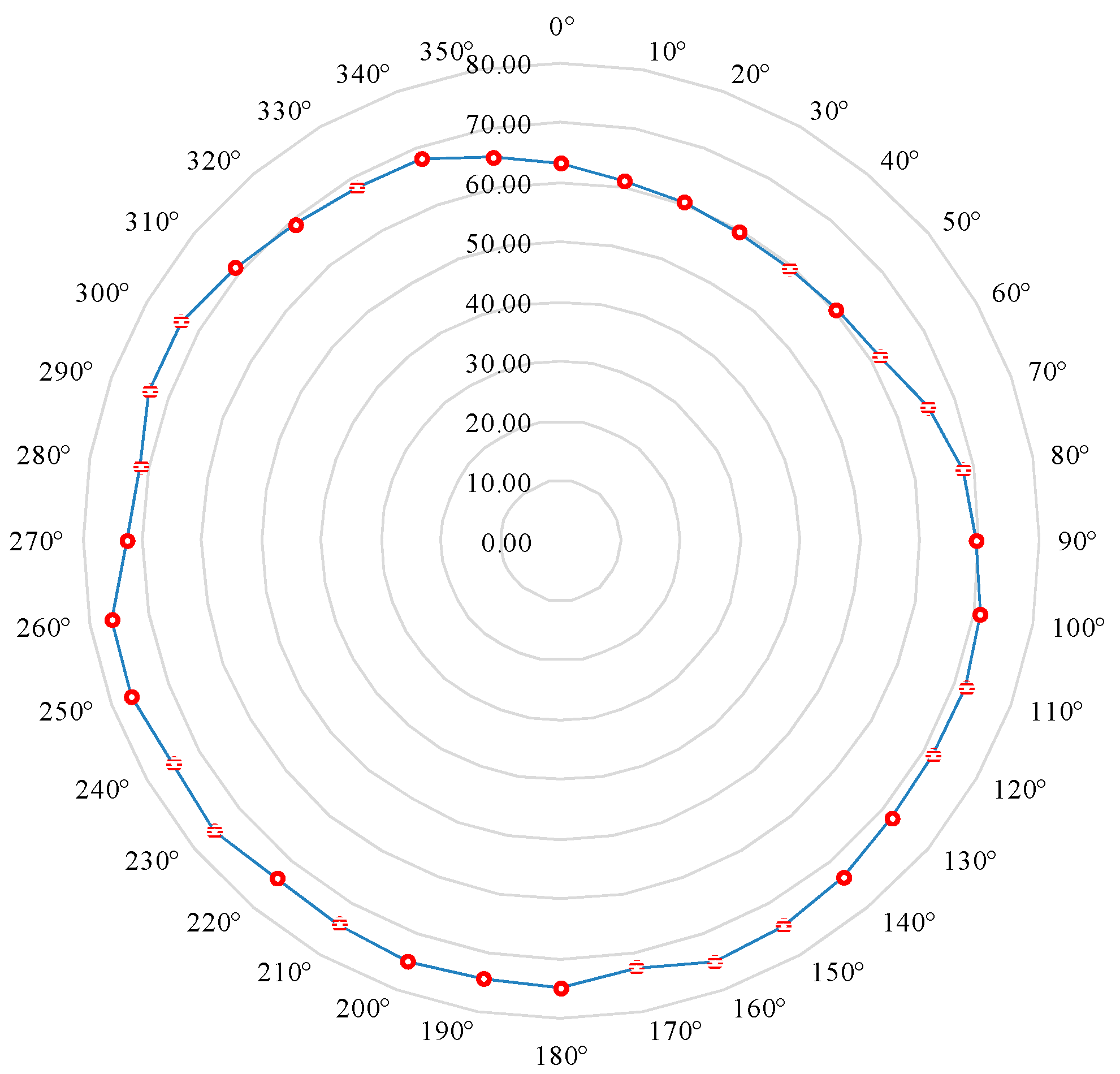
3.2. Operating Point

The characteristic curves of the pumping station (Q-H_p, Q-η_p, and Q-P_Abs), adjusted through data taken from the manufacturer, are shown in Figure 5. The operating point of the index characteristic curve “f”, relative to the configuration of the pumping unit with a fixed speed is shown. In addition, the operating point of the index characteristic curve “v” refers to the configuration with a variable speed. In both cases, the angular position of the lateral line of 40° was represented with the fixed speed (n_f = 1750 rpm and α = 1.00) and variable speed pump (n_v = 1523 rpm and α = 0.85). This position was chosen because it has a minor pressure head value.

In Figure 5, it can be seen that the displacement of curves (Q-H_p)_v and (Q-P_Abs)_v to (Q-H_p)_f and (Q-P_Abs)_f did not result in significant differences in pump efficiency (Q-η_p)_f,v. This result demonstrates that the use of the VSD in the irrigation system does not significantly interfere with the pump efficiency, whose high and low values were close to 80.26% (α = 0.85) and 78.54% (α = 1.00). This displacement also demonstrates the reduction of energy consumption (12.2%) through the influence of the VSD on the pumping station of the irrigation system under study. This same behavior of curve displacement was reported by Brar et al. [20] in a study on energy efficiency in center pivots. They determined that by reducing the speed of the pumping station’s rotation through the VSD, it was possible to reduce its head pressure, thereby maintaining the efficiency of the pump. Also, as described by Córcoles et al. [27], the ratio (in kWh m⁻³) can be higher at lower frequencies than the nominal value, thus presenting another source of energy saving.

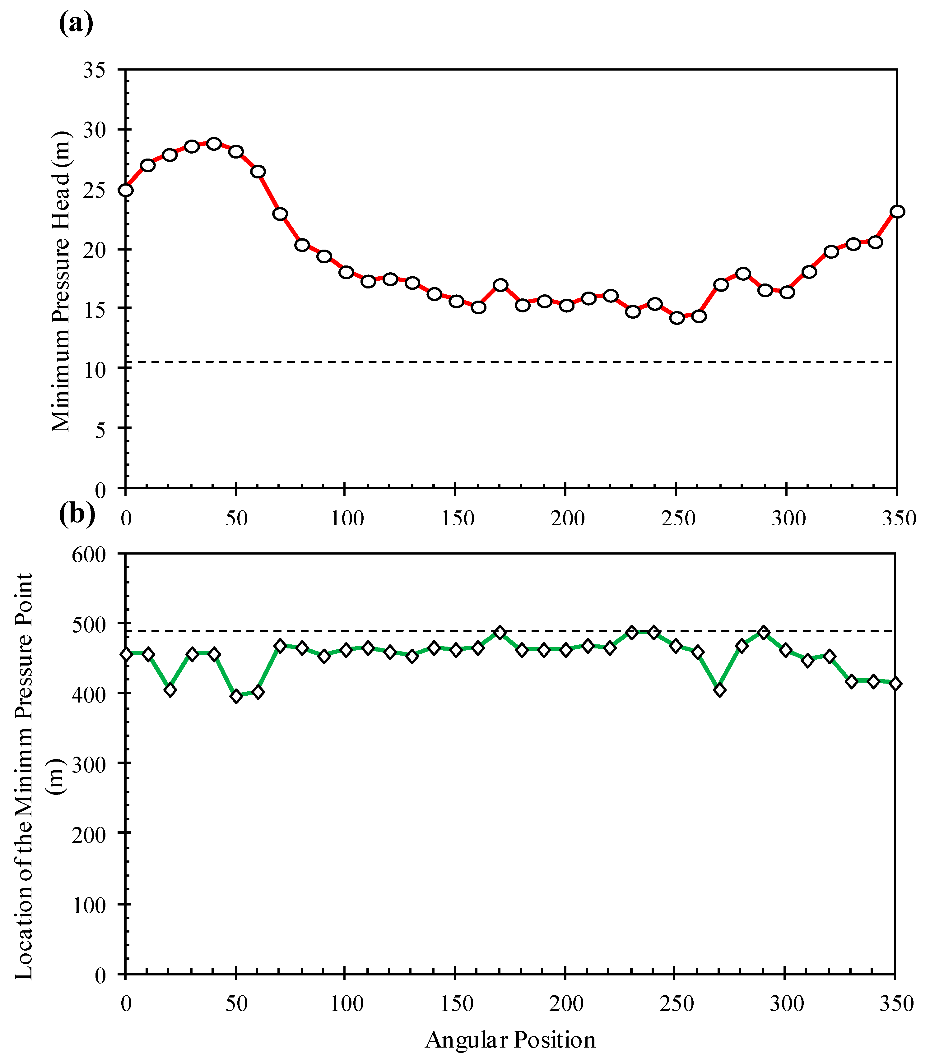
3.3. Pressure Distribution Along the Lateral Line

After the hydraulic simulation of the center pivot, the pressure values at the top of the lateral line were obtained for each angular position at the nodes referring to the water outlets. Thus, the minimum pressure head value corresponds to the minor value of the pressure distribution. The pump speed computed at each angular position was the minimum pump speed that was able to keep pressure values at the downstream node of every PRV equal to the setting pressure (ie keeping every PRV at the Partially closed state). So, according to EPANET PRV rules described above, this condition was achieved when pressure values at every PRV upstream node were above the setting pressure. The minimum pressure head values and the location of the minimum pressure head along the lateral line are shown in Figure 6.

According to [13,20,21], the point of minimum pressure is located between the end of the lateral line and the center of the pivot according to the topographic changes of the irrigated area.

King et al. [13], studying the spatial distribution of pressure on the lateral portion of a center pivot (with a length of 392 m and a difference in the level of 18 m), reported that the point of minor pressure on the lateral line was not necessarily situated at the end. The location of that point was variable according to the different slopes of the irrigated area. This fact made it difficult to install pressure sensors to control the speed of the pumping station with a VSD.

Figure 6 also shows the location of the point of minimum pressure with respect to the end of the lateral line. In some angular positions, the minimum pressure value is located exactly at the end of the lateral line. This result shows the influence of the small topographic differences of the irrigated area on the location of the minimum pressure point and, consequently, on the potential reduction of energy consumption.

3.4. Energy Analysis

Pumping stations are designed for the lateral line’s most critical angular position, i.e., the position where the lateral line has the largest positive level difference. Thus, the minimum pressure head is located at the lateral end. Pumping station values for the different lateral line angular positions and values for the fixed speed pump are shown in

Table 1. Flow rate (Q), pumping pressure head (H_i), hydraulic power (P_H), speed of the pumping station (n), variable speed ratio (α), efficiencies (η), and specific energy consumption (CEE) in the different angular positions of the lateral line.

Angular Position	Q (m3 h−1)	Hi (m)	PH (kW)	n	α	ηp (%)	ηm (%)	ηv (%)	ηc (%)	ηt 1 (%)	CEE (kWh m−3)
Fixed	326.61	65.23	58.04	1750	1.00	78.54	94.13		98.60	72.90	0.244*
0°	326.61	50.72	45.12	1574	0.90	80.08	93.86	96.75	98.65	71.74	0.193
10°	326.61	48.64	43.27	1547	0.88	80.20	93.77	96.21	98.66	71.38	0.186
20°	326.61	47.77	42.50	1535	0.88	80.23	93.73	95.95	98.66	71.19	0.183
30°	326.61	47.07	41.88	1526	0.87	80.26	93.69	95.71	98.66	71.01	0.181
40°	326.61	46.84	41.67	1523	0.87	80.26	93.68	95.63	98.67	70.94	0.180
50°	326.61	47.49	42.25	1531	0.88	80.24	93.71	95.86	98.66	71.12	0.182
60°	326.61	49.16	43.74	1553	0.89	80.17	93.79	96.36	98.66	71.48	0.187
70°	326.61	52.69	46.88	1599	0.91	79.93	93.93	97.13	98.64	71.93	0.200
80°	326.61	55.29	49.20	1631	0.93	79.70	94.00	97.43	98.63	72.00	0.209
90°	326.61	56.24	50.04	1643	0.94	79.61	94.02	97.48	98.63	71.96	0.213
100°	326.61	57.57	51.22	1659	0.95	79.47	94.04	97.51	98.63	71.88	0.218
110°	326.61	58.33	51.90	1669	0.95	79.39	94.05	97.50	98.62	71.80	0.221
120°	326.61	58.15	51.73	1666	0.95	79.41	94.05	97.50	98.62	71.82	0.221
130°	326.61	58.45	52.01	1670	0.95	79.38	94.06	97.50	98.62	71.79	0.222
140°	326.61	59.38	52.83	1681	0.96	79.27	94.07	97.45	98.62	71.67	0.226
150°	326.61	60.00	53.38	1689	0.96	79.20	94.08	97.41	98.62	71.58	0.228
160°	326.61	60.49	53.82	1695	0.97	79.14	94.09	97.37	98.62	71.49	0.230
170°	326.61	58.63	52.16	1672	0.96	79.36	94.06	97.49	98.62	71.77	0.223
180°	326.61	60.33	53.67	1693	0.97	79.16	94.08	97.38	98.62	71.52	0.230
190°	326.61	59.99	53.37	1688	0.96	79.20	94.08	97.41	98.62	71.58	0.228
200°	326.61	60.35	53.69	1693	0.97	79.16	94.08	97.38	98.62	71.52	0.230
210°	326.61	59.75	53.16	1686	0.96	79.23	94.08	97.43	98.62	71.61	0.227
220°	326.61	59.52	52.96	1683	0.96	79.25	94.07	97.44	98.62	71.65	0.226
230°	326.61	60.86	54.15	1699	0.97	79.10	94.09	97.33	98.62	71.43	0.232
240°	326.61	60.21	53.57	1691	0.97	79.17	94.08	97.39	98.62	71.54	0.229
250°	326.61	61.37	54.60	1705	0.97	79.03	94.10	97.27	98.61	71.33	0.234
260°	326.61	61.24	54.48	1703	0.97	79.05	94.09	97.28	98.61	71.36	0.234
270°	326.61	58.61	52.15	1672	0.96	79.36	94.06	97.49	98.62	71.77	0.222
280°	326.61	57.68	51.32	1661	0.95	79.46	94.04	97.51	98.63	71.87	0.219
290°	326.61	59.07	52.56	1677	0.96	79.31	94.07	97.47	98.62	71.71	0.224
300°	326.61	59.24	52.70	1679	0.96	79.29	94.07	97.46	98.62	71.69	0.225
310°	326.61	57.53	51.19	1659	0.95	79.48	94.04	97.51	98.63	71.88	0.218
320°	326.61	55.85	49.69	1638	0.94	79.65	94.01	97.47	98.63	71.98	0.211
330°	326.61	55.22	49.13	1630	0.93	79.71	93.99	97.42	98.63	72.00	0.209
340°	326.61	55.05	48.98	1628	0.93	79.73	93.99	97.41	98.63	72.00	0.208
350°	326.61	52.50	46.71	1596	0.91	79.95	93.92	97.10	98.64	71.92	0.199

¹ Total efficiency * variable speed drives (VSDs) efficiency not considered.

.

In Table 1, it can be sheen that the i = 40° position (Figure 4) has the lowest pumping pressure head value (46.84 m) and, consequently, a lower specific energy consumption value (0.180 kWh m⁻³). On the other hand, position I = 250° presents the highest values−61.37 m and 0.234 kWh m⁻³, respectively. It should be noted that for these positions, the determination of the CEE with the variable speed of the pump is different from the CEE with a fixed speed, because, in this configuration, the value of VSD efficiency is not considered.

Specific energy consumption (kWh m⁻³) values for the fixed speed (without VSD) and variable speed (with VSD) pumping stations were determined. The specific energy consumption using the VSD was computed as the average values considering all the angular positions of the lateral line. In general, due to the small variations in the topography of the irrigated area, the average value of the CEE with variable speed of the pumping station was close to the value of the CEE with a fixed speed (0.214 and 0.244 kWh m⁻³, respectively), resulting in an energy reduction value of 12.2%. This percentage is lower than the values found by [18] (32% energy savings using variable speed well pumps in a center pivot system), [19] (27% to 35% of energy savings can be achieved using VSD in two Italian irrigation districts operating with three parallel horizontal axis pumps), and higher than those found by Brar et al. [20] (9.6% energy reduction is possible for 13.6 m difference in the irrigated area for a study containing 100 center pivots in Nebraska (USA), with each pivot containing a pumping station). However, these studies did not take into account the efficiency of VSD. The energy reduction value of this study is close to that found by King et al. [13] (7.5% to 15.8%), who considered the variable speed drive efficiency of a center pivot pumping unit. This result demonstrates that using VSD can reduce energy consumption in pumping units for water distribution.

In the present study, the center pivot system is equipped with a single pump. The use of VSDs in situations where multiple pumps supply several irrigation systems can result in greater energy savings, as can be seen in the studies conducted by [18,19].

The values of the absorbed power (the relation of the hydraulic power and total efficiency, in kW) at the pumping station at each of the angular positions of the center pivot’s lateral line are shown in Figure 7.

In Figure 7, the lowest values of the absorbed power (51.92 kW) were reached in the angular positions where the lateral line assumes a downward slope (i = 40°) from the center to the end. In the same way, when the lateral line presents an ascending slope (i = 250°), it results in higher values of absorbed power (69.09 kW). This difference in values results in a reduction of 28.5% between these two angular positions. It should be noted that the total efficiency of these two positions is very close (70.9% (for i = 40°) and 71.3% (for i = 250°)). These results are directly related to the movement of the point of minimum pressure along the lateral line according to topographic variations of the irrigated area. The same type of behavior for the minimum pressure point was reported by Brar et al. [20] and King et al. [13] in studies with energy conservation in the center pivot systems using variable speed drives at the pumping station.

3.5. Economic Analysis

To analyze the operation costs with the use of VSDs in this center pivot, the values of energy consumption and costs, considering the two configurations (fixed and variable speed) for an irrigation season with maize crop in the region of Albacete (Spain), are presented in

Table 2. The consumption and cost of energy for the pumping stations with fixed and variable speeds.

Crop		Maize
GIWR (gross irrigation water requirement)	mm	627.00
Flow rate	m3 h−1	326.61
Operation time	h	1440.00
ECf	kWh	114739.03
ECv	kWh	100632.47
Average cost	€ kW h−1	0.20
Cf	€	22947.96
Cv	€	20126.49
Energy Savings	€ year−1	2821.47

.

For an irrigated area with a maximum elevation difference of 15.3 m, and considering the use of a VSD with a fixed speed, the annual average energy savings is close to 14107.35 kWh (Table 2), representing an annual average energy cost savings of 2821.47€.

In a similar study, [13] presented an average annual saving of 18100.00 kWh, applying a requirement of 635 mm of gross water irrigation and an area with an elevation difference of 18 m. They concluded that the VSD installation would not be economically viable. This result can be explained due to the low performance of the utility’s equipment and the low cost of energy (0.031 kWh⁻¹) in the region where the study was conducted, which resulted in a low average annual saving (564.30 €). The average annual energy savings (kWh) presented by [13] were similar to those determined in the present study. However, due to the unit cost of energy consumption, the financial savings were lower. This fact shows that the cost of energy, besides the topography of the irrigated area, must be taken into account for this type of analysis.

Working with several center pivots for the maize crop, Brar et al. [20] presented an average annual saving of 4155 kWh, applying a requirement of 284 mm of gross water irrigation to an average irrigated area of 49 ha with a height difference of 13.6 m. The average pumping cost was 0.098 kWh⁻¹, resulting in average annual savings of 407.40€. The difference of the values in this study can be explained by the smaller difference in elevation, their low energy cost, and their lower gross irrigation requirements.

4. Conclusions

This study presented a proposal to vary the pressure supplied to a center pivot irrigation system according to the angular position of the lateral line by adjusting the speed of the pumping station with a variable speed drive (VSD). A model was developed to simulate the possible reduction in energy consumption when using a VSD in a center pivot pumping station in Albacete (Spain). For topographic characterization, DEMs from satellite images (with 5 × 5 m spatial accuracy) were used, and it was concluded that the topographic precision for this type of study is essential to determine the required pressure values at each angular position of the center pivot’s lateral line.

The present study showed a saving of 12.2% of energy when using speed control at the pumping station in comparison with the commonly used fixed speed. This reduction in energy allowed economic savings close to 2821.47 €, in an area irrigated by a center pivot with a difference in maximum elevation of 15.3 m and the major part of the lateral line on the ascending slope.

The VSPM tool, which added topographic, hydraulic, and energy characteristics to the irrigation system, facilitated the simulation of the center pivot irrigation system in the EPANET software, along with the analyses of the use of VSD in the speed control of the pumping station. This tool demonstrates the possible financial return when using a VSD in a center pivot pumping station that operates in areas of variable topography. This center pivot represents the greater part of the irrigated area in the ascending slope during the movement of the lateral line. Therefore, for an irrigated area where the lateral line remains in a descending slope during the greater part of its rotation, the energy savings would be greater. Thus, this tool seems to be useful for users to achieve better precision in energy and economic analyses of center pivot irrigation systems.

The use of VSD to control the speed of the pumping station of the irrigation system showed a greater reduction in energy consumption when the different angular positions of the lateral line along the irrigated area were in an ascending slope. In these positions, the point of minimum pressure tends to migrate from the extremity to the center of the pivot.

This study aimed to quantify the energy saving potential of VSDs, providing irrigation producers and professionals results that show the benefits of installing VSDs in the pumping stations of center pivot irrigation systems.

References

1. Alexandratos, N.; Bruinsma, J. World Agriculture Towards 2030/2050: The 2012 Revision; ESA Work. Pap. No. 12–03; FAO: Rome, Italy, 2012; p. 153. [Google Scholar]
2. Pereira, L.S. Water, Agriculture and Food: Challenges and Issues. Water Resour. Manag. 2017, 31, 2985–2999. [Google Scholar] [CrossRef]
3. World Business Council for Sustainable Development. Water, Food and Energy Nexus Challenges; World Business Council for Sustainable Development: Geneve, Switzlerand, 2014. [Google Scholar]
4. Tarjuelo, J.M.; Rodriguez-diaz, J.A.; Abadía, R.; Camacho, E.; Rocamora, C.; Moreno, M.A. Efficient water and energy use in irrigation modernization: Lessons from Spanish case studies. Agric. Water Manag. 2015, 162, 67–77. [Google Scholar] [CrossRef]
5. AQUASTAT Database. FAO’s Global Water Information System: Area Equipped for Irrigation; FAO: Rome, Italy, 2014. [Google Scholar]
6. Frizzone, J.A.; Rezende, R.; Camargo, A.P.; Colombo, A. Irrigação por Aspersão: Sistema Pivô Central, 1st ed.; Editora UEM: Maringá, PR, Brazil, 2018. [Google Scholar]
7. Keller, J.; Bliesner, R.D. Sprinkle and Trickle Irrigation; Van Nostrand Reinholh: New York, NY, USA, 1990. [Google Scholar]
8. Folegatti, M.V.; Pessoa, P.C.S.; Paz, V.P.S. Avaliação do desempenho de um Pivô Central de Grande Porte e Baixa Pressão. Sci. Agric. 1998, 55, 119–127. [Google Scholar] [CrossRef]
9. Gilley, J.R.; Watts, D.G. Possible Energy Savings in Irrigation. J. Irrig. Drain. Div. 1977, 103, 445–457. [Google Scholar]
10. Moreno, M.A.; Planells, P.; Córcoles, J.I.; Tarjuelo, J.M.; Carrión, P.A. Development of a new methodology to obtain the characteristic pump curves that minimize the total cost at pumping stations. Biosyst. Eng. 2008, 102, 95–105. [Google Scholar] [CrossRef]
11. Moreno, M.A.; Medina, D.; Ortega, J.F.; Tarjuelo, J.M. Optimal design of center pivot systems with water supplied from wells. Agric. Water Manag. 2012, 107, 112–121. [Google Scholar] [CrossRef]
12. Barbosa, B.D.S.; Colombo, A.; de Souza, J.G.N.; da Baptista, V.B.; de Araújo, A.C.S. Energy Efficiency of a Center Pivot Irrigation System. Eng. Agrícola 2018, 38, 284–292. [Google Scholar] [CrossRef]
13. King, B.A.; Wall, R.W. Distributed Instrumentation for Optimum Control of Variable Speed Eletric Pumping Plants with Center Pivots. Appl. Eng. Agric. 2000, 16, 45–50. [Google Scholar] [CrossRef]
14. Kranz, W.L.; Irmak, S.; Martin, D.L.; Yonts, C.D. Flow Control Devices for Center Pivot Irrigation Systems. Univ. Neb. Linc. Ext. Inst. Agric. Nat. Resour. 2007, 888, 1–3. [Google Scholar]
15. Alandi, P.P.; Pérez, P.C.; Álvarez, J.F.O.; Moreno, M.Á.; Tarjuelo, J.M. Pumping Selection and Regulation for Water-Distribution Networks. J. Irrig. Drain. Eng. 2005, 131, 273–281. [Google Scholar] [CrossRef]
16. Khadra, R.; Moreno, M.A.; Awada, H.; Lamaddalena, N. Energy and Hydraulic Performance-Based Management of Large-Scale Pressurized Irrigation Systems. Water Resour. Manag. 2016, 30, 3493–3506. [Google Scholar] [CrossRef]
17. Fernández García, I.; Moreno, M.A.; Rodríguez Díaz, J.A. Optimum pumping station management for irrigation networks sectoring: Case of Bembezar MI (Spain). Agric. Water Manag. 2014, 144, 150–158. [Google Scholar] [CrossRef]
18. Hanson, B.R.; Weigand, C.; Orloff, S. Variable-frequency drives for electric irrigation pumping plants save energy. Calif. Agric. 1996, 50, 36–39. [Google Scholar] [CrossRef]
19. Lamaddalena, N.; Khila, S. Energy saving with variable speed pumps in on-demand irrigation systems. Irrig. Sci. 2012, 30, 157–166. [Google Scholar] [CrossRef]
20. Brar, D.; Kranz, W.L.; Lo, T.; Irmak, S.; Martin, D.L. Energy Conservation Using Variable-Frequency Drives for Center-Pivot Irrigation: Standard Systems. Trans. ASABE 2017, 60, 95–106. [Google Scholar] [CrossRef]
21. Scaloppi, E.J.; Allen, R.G. Hydraulics of Center Pivot Laterals. J. Irrig. Drain. Eng. 1993, 119, 554–567. [Google Scholar] [CrossRef]
22. Moreno, M.A.; Córcoles, J.I.; Tarjuelo, J.M.; Ortega, J.F. Energy efficiency of pressurised irrigation networks managed on-demand and under a rotation schedule. Biosyst. Eng. 2010, 107, 349–363. [Google Scholar] [CrossRef]
23. Rossman, L.A. EPANET 2: User Manual; National Risk Management Research Laboratory Office of Research and Development, U.S. Environmental Protection Agency: Cincinnati, OH, USA, 2000.
24. Valiantzas, J.D.; Dercas, N. Hydraulic Analysis of Multidiameter Center-Pivot Sprinkler Laterals. J. Irrig. Drain. Eng. 2005, 131, 137–146. [Google Scholar] [CrossRef]
25. Bernier, M.A.; Bourret, B. Pumping energy and variable frequency drives. ASHRAE J. 1999, 41, 37–40. [Google Scholar]
26. Alazba, A.A.; Asce, M.; Mattar, M.A.; Elnesr, M.N.; Amin, M.T. Field Assessment of Friction Head Loss and Friction Correction Factor Equations. J. Irrig. Drain. Eng. 2012, 138, 166–176. [Google Scholar] [CrossRef] [Green Version]
27. Córcoles, J.; Gonzalez Perea, R.; Izquiel, A.; Moreno, M. Decision Support System Tool to Reduce the Energy Consumption of Water Abstraction from Aquifers for Irrigation. Water 2019, 11, 323. [Google Scholar] [CrossRef]
Figure 1. Diagram of the proposed procedure.
Water 11 02192 g001
Figure 2. The geographic coordinates during the rotation of the lateral line at the center pivot.
Water 11 02192 g002
Figure 3. (a) Center pivot lateral line span dimensions, (b) EPANET network map of the first span of the center pivot lateral line.
Water 11 02192 g003
Figure 4. Network maps of the center pivot system from EPANET inp files generated by the VSPM (Variable Speed Pivot Model) tool considering two different lateral line angular positions (a) 250° uphill and (b) 40° downhill.
Water 11 02192 g004
Figure 5. Pumping station characteristic curves for the 40° angular position lateral line with a fixed speed (f) and variable speed (v), (a) (Q-H) and (Q-η) curves, (b) (Q-PAbs) curve.
Water 11 02192 g005
Figure 6. (a) Value and (b) location of the point of minimum pressure head in the different angular positions of the center pivot lateral line.
Water 11 02192 g006
Figure 7. Absorbed power at the pumping station for the different angular positions of the lateral line.
Water 11 02192 g007