Dewatering Characteristics and Inflow Prediction of Deep Foundation Pits with Partial Penetrating Curtains in Sand and Gravel Strata


1
School of Civil Engineering, Central South University, Changsha 410075, China
2
Key Laboratory of Engineering Structure of Heavy Haul Railway, Central South University, Changsha 410075, China
*
Authors to whom correspondence should be addressed.
Water 2019, 11(10), 2182; https://doi.org/10.3390/w11102182
Submission received: 2 September 2019
/
Revised: 15 October 2019
/
Accepted: 17 October 2019
/
Published: 19 October 2019
(This article belongs to the Special Issue Modeling of Flow and Transport in Saturated and Unsaturated Porous Media)
Abstract
:The dewatering of deep foundation pits excavated in highly permeable geology usually requires waterproofing technologies to relieve groundwater flow. However, no effective prediction formula is yet available for determining water inflow in the presence of partial penetrating curtains. In this study, a dewatering project with partial penetrating curtains is analyzed via a finite difference method to show evident three-dimensional (3D) seepage characteristics. The standard curve and distortion functions are established under the assumption of an equivalent well by quantifying the blocking effects; thus, the empirical inflow prediction formulas for steady flow are further developed. Moreover, a dewatering design method based on the prediction formulas is proposed and applied to the field dewatering project in sand and gravel strata. Measured results show that dewatering efficiency is considerably enhanced by 3D flow, forming appropriate pressure distributions for dewatering construction. The uplift pressure below the pit bottom is controlled within a 25% safety margin to verify the reliability of the design method.
1. Introduction
Social problems caused by the accelerated urbanization process, such as ground space congestion and rapid population growth, have persistently afflicted urban development. To solve these issues, numerous underground infrastructures (e.g., metro tunnels, stations) have been built using deep foundation pit technology [1]. Most excavation depths in urban areas have reached more than 20 m at present [2,3]. In the eastern coastal areas of China (e.g., Shanghai, Tianjin, and Hangzhou), considerable amounts of Quaternary marine and estuarine sediments have been alternately deposited, forming an alternating multi-aquifer system (MAS) composed of low-permeability clay, silt, saturated sand, and gravel layers [4,5,6,7]. Besides, these deposits frequently have high water tables as approaching the coast [8,9]. Thus, the excavation surface is commonly below the groundwater surface in such areas. For excavation stability, a dry construction environment is necessary, so groundwater control measures are supposed to be adopted during construction. However, the stratigraphic distribution of several MAS regions (such as Fuzhou City) is heterogeneous and discontinuous [10,11]. The voids or deficiencies of aquitards form hydraulic connections among aquifers and provide strong recharge capacity; in such cases, maintaining dry excavation conditions may be extremely difficult. Furthermore, the high water pressure may cause engineering disasters; for example, when overlying layers are excavated, the exposed pit bottom may suffer from groundwater uplift action, resulting in bottom uplift failure and even water inflowing towards the excavation [12,13]. Thus, groundwater pressure around a pit must be controlled by reasonable methods.
The dewatering decompression method has been commonly applied to the groundwater pressure control so far [14]; however, drawdowns caused by excessive pumping may lead to the development of a depression cone around a pit that further induces pore compression of the aquitard and forms ground settlements [15,16,17,18,19]. Thus, waterproofing technology has been used to alleviate water flow during dewatering by utilizing low-permeability curtains, such as deep mixing piles [20,21], jet grouting piles [22,23], diaphragm walls [24], and other structures that can fully or partially block seepage. However, defects frequently occur at the full penetrating wall with a long penetrating length [25,26] and lead to partial leakage, causing ground collapse and endangering the safety of surrounding buildings. Thick aquifers limit the utilization of the full penetrating wall and other partial penetrating wall schemes are accepted in the field.
The dewatering design of deep foundation pits with partial penetrating curtains has been widely researched in recent years. Many studies have focused on settlement control and blocking effects via numerical and field test methods [27,28,29,30,31,32]. Studies have shown that curtains in the seepage field change flow direction, path, and section and also increase the hydraulic gradient. The combination of partial penetrating wells and curtains can form a complex three-dimensional (3D) seepage field, and the coupled non-Darcy flow further consumes seepage energy [33,34]. The anisotropy of aquifer permeability can also enhance dewatering efficiency [35]. The coupled wall–well effect has been further studied with the maturity of experimental methods [36,37], and scale experiments have been performed to verify the coupled effect and explore optimal wall–well locations. These studies have gradually explored the seepage mechanism of partial penetrating curtains and provided scientific design recommendations. At present, the numerical method is commonly applied to dewatering designs of deep excavations with partial penetrating walls. However, this design method is not efficient due to its modeling complexity that requires considerable calculation effort. Formalized inflow prediction formulas are necessary to ensure the reliability of designs. However, no analytical solution is yet available because of the complex 3D seepage field caused by partial penetrating curtains. Thus, the current study aims to quantify the blocking effect and propose inflow prediction formulas for foundation pits with partial penetrating curtains. Furthermore, a corresponding design method is presented in this paper.
2. Problem Description
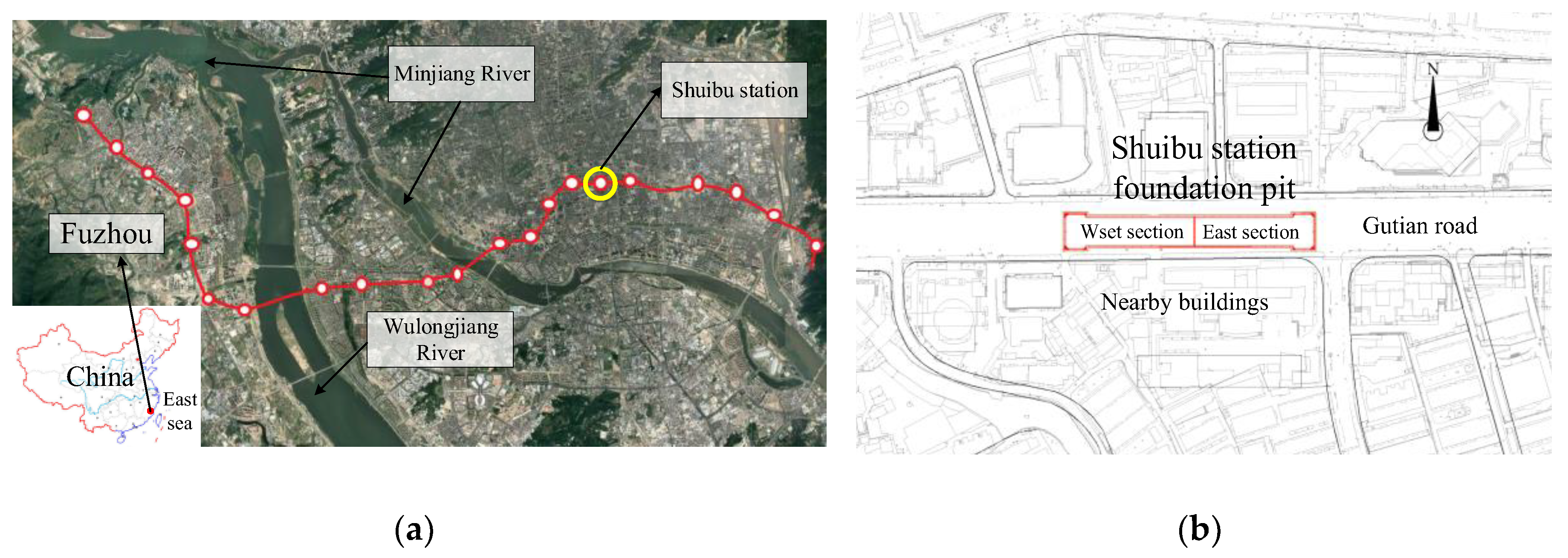
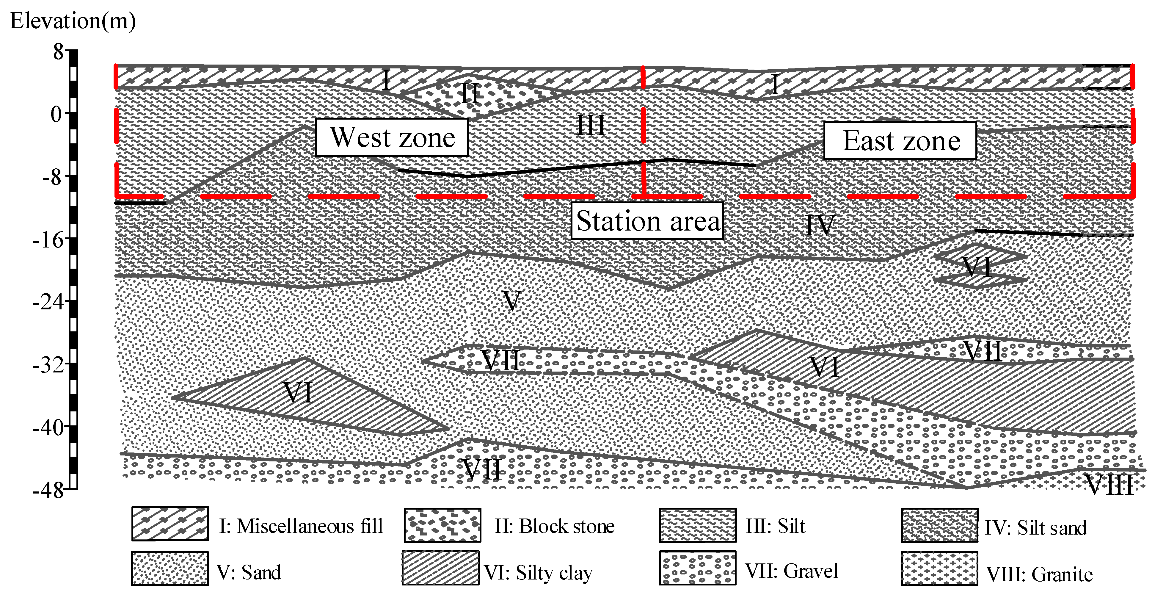
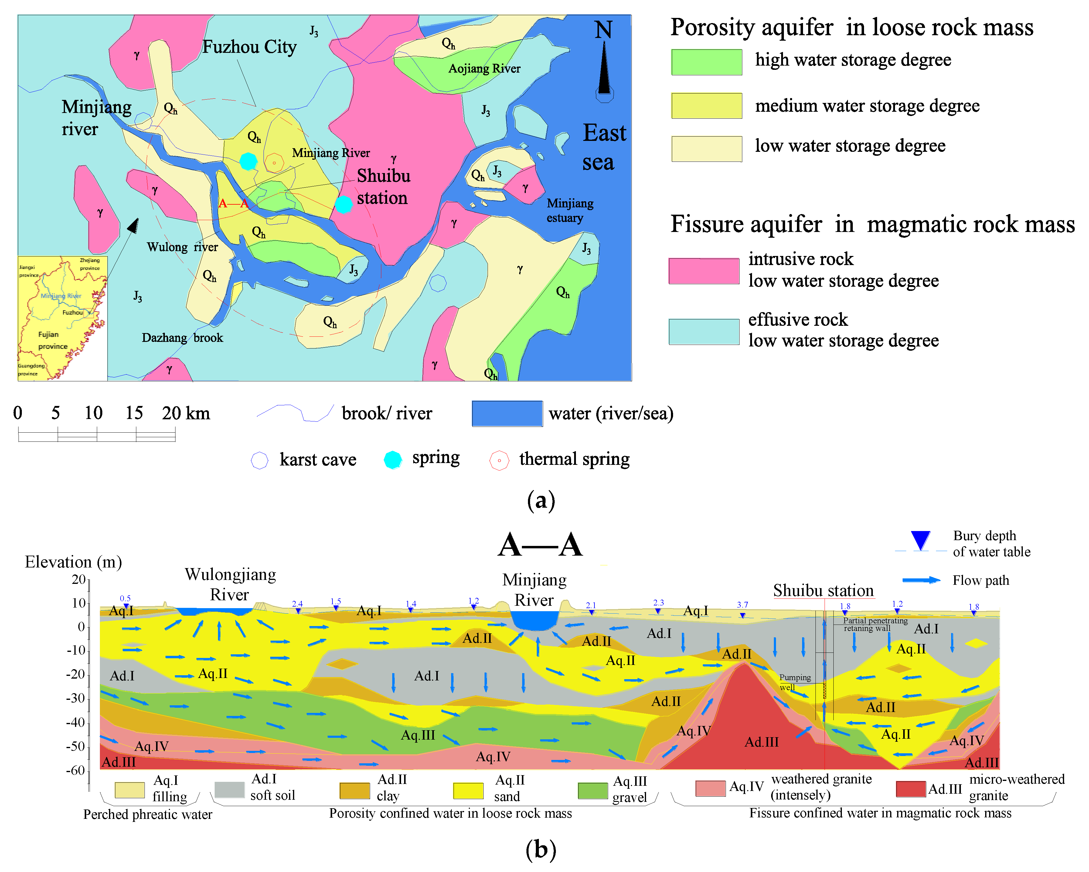
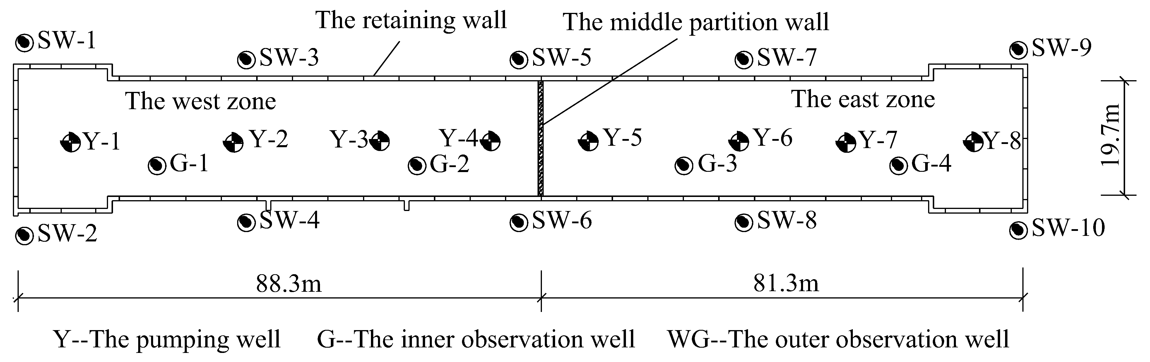
This investigation is performed on typical layered strata in Fuzhou City. The geographical location of the study area is presented in Figure 1. Figure 2 shows the longitudinal sectional view of the strata distribution of the station. The confined and phreatic aquifers within regions with an overall thickness of 56 m are separated by the upper aquitard (III: silt). The phreatic layer is mostly composed of miscellaneous fill with blocked hydraulic connections to confined aquifers. A confined aquifer is composed of layered sand (V) and gravel (VII) layers. The gravel layer generates a hydraulic connection with the sand layer through the ‘connected area’ of the incompletely sealed lower aquitard (VI: silty clay). This area is intermittently distributed at the bottom of the sand layer, and it produces a strong hydraulic recharge that exerts considerable impact on excavations. All of the formation parameters in the field are listed in Table 1. The metro station foundation pit is 169.6 m long and 19.7 m wide, with a pit bottom bury depth of 16.5 m. This foundation pit is long and narrow but equally divided into two sections by the middle wall. The pit bottom is located in the silty sand (IV) layer above the confined aquifers. The overlying soil pressure decreases with an increase in excavation depth, posing a risk of uplift failure below the excavation surface.
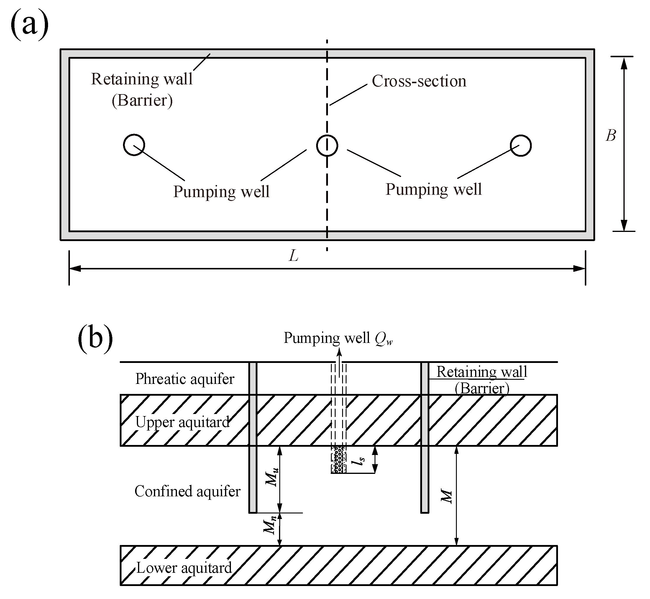
To investigate seepage characteristics, the pit section is simplified into a rectangular section. Figure 3 shows the problem sketch. In general, the 4th dewatering model (ls < Mu) is selected for dewatering projects in deep aquifers [24]. With a fixed Qw and increasing elapsed time t, the hydraulic head dramatically decreases from its initial position until it finally reaches a stable value [35]. This study aims to explore steady seepage characteristics under partial penetrating curtains in the 4th dewatering model and to establish formalized Qw prediction formulas for a dewatering design. Furthermore, the corresponding dewatering design method shall be presented on the basis of these formulas.
3. Numerical Simulation
3.1. Governing Equation
To obtain the conservative inflow design value, non-Darcy flow is disregarded, but the assumption of Darcy’s law and the continuity condition are adopted. The governing equation and boundary conditions of 3D groundwater seepage in the saturated media of confined aquifers are established as follows [38]:
where ∇ is the Laplace operator; kij is the permeability coefficient, and i, j, = 1, 2, 3; h is the hydraulic head; Q is the external source–sink flux; Ss is the specific storage; t is the elapsed time; h0(x, y, z) is the initial head at point (x, y, z); h1(x, y, z, t) is the constant head on boundary Γ1; nx, ny, and nz are the unit normal vector on boundary Γ2 along the x, y, and z directions, respectively; q(x, y, z, t) is the lateral recharge per unit area on boundary Γ2; Γ1 is the boundary condition of the water table; and Γ2 is the flux boundary condition.
When the 3D seepage field approaches a steady state, the flow rate of boundary elements tends to be 0. The governing equation of Equation (1) can be written as follows:
Aquifers are commonly heterogeneous along the vertical direction and homogeneous along the horizontal direction. Therefore, Equation (2) is rewritten as:
where kh is the horizontal permeability coefficient, and kv is the vertical permeability coefficient.
At present, the preceding governing equations have no analytic solution yet because of the blocking effect. Hence, a finite difference method (FDM) can be applied. The seepage field is discretized into 3D cells, and then the difference equation is established at the cell (i, j, k) as follows [39]:
where is the head of the cell (i, j, k) at the time step m, (L); CR, CC, and CV are the hydraulic conductivity between adjacent nodes (L2 T−1); Pi, j, k is the sum of the head coefficients between the source and the sink (L2/T); and Qi, j, k is the sum of the constants of the source and the sink (L3/T). When Qi, j, k < 0, groundwater is exiting the system (e.g., pumping); when Qi, j, k > 0, groundwater is entering the system (e.g., injection). Si, j, k is the cell’s specific storage. ∆rj, ∆cj, and ∆vj are the 3D dimensions of the cube cell (i, j, k). tm is the time in time step m (T). To represent the hydraulic gradient between nodes rather than the hydraulic gradient between cells, the subscript symbol “1/2” is adopted. For the steady flow that governs Equation (2), the storage term at the right side of the difference equation, i.e., Equation (4), is set to 0 to establish the corresponding difference equation.
The calculation domain of seepage is discretized into a difference grid on the basis of Equation (4), and then the head of each element can be solved using an iterative algorithm [40].
3.2. Simplification of Model Parameters
The numerical model is established on the basis of Equation (4). To investigate seepage characteristics, all of the field strata are summarized as three main layers in the model: The phreatic, aquitard, and confined aquifers. Table 2 provides the simplified parameters in the calculation model on the basis of the Fuzhou strata. The typical size of a rectangle station pit section is adopted in the calculation: L = 60 m, B = 20 m, and the depth of the retaining wall is 42 m (Mu = 18 m) with a short screen length of 8 m. Notably, the aforementioned parameters can be changed individually in accordance with the requirement.
3.3. Initial/Boundary Conditions
To avoid the boundary effect, Siechardt’s empirical formula is applied to calculate the pumping influence radius, as follows [38]:
where sw is the drawdown of the pumping well, and k is the aquifer’s permeability coefficient.
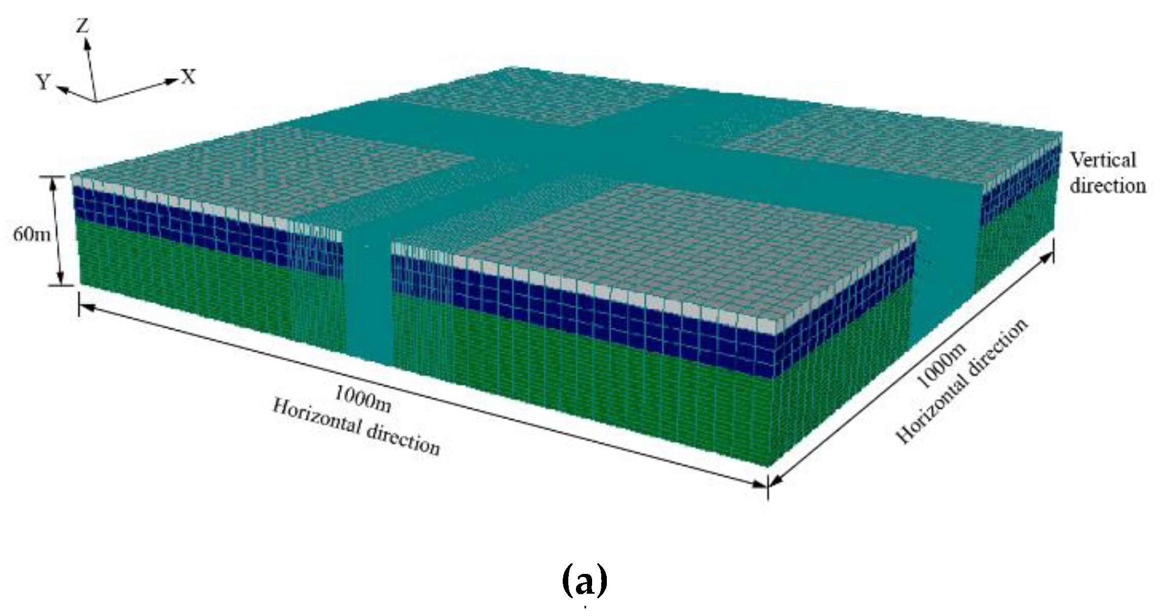
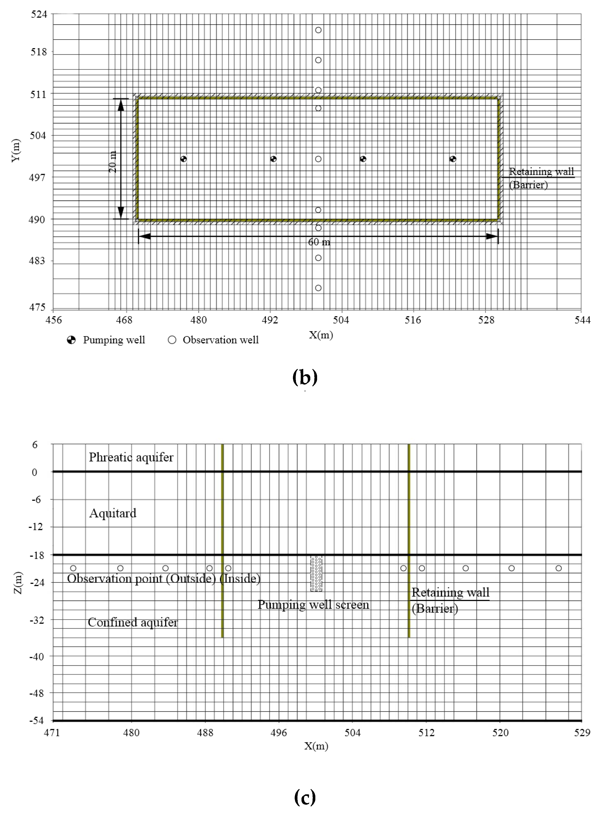
Assume that the required sw is approximately 8 m and the maximum permeability coefficient of a confined aquifer k is 36 m/d based on field conditions. The influence radius R is calculated as 480 m using Equation (5). The model range is supposed to extend to more than 480 m from the pit center. Then, a 1000-m-long, 1000-m-wide, and 60-m-deep FDM mesh is obtained. As shown in Figure 4, the horizontal direction has 129 rows and 141 columns. A fine mesh is found around the excavation area and gradually becomes a coarse mesh from the excavation center outward. In the vertical direction, the model of the three strata is divided into 22 layers and the confined aquifer is calculated in 18 layers.
Taking the ground surface as the reference datum, the initial hydraulic head of the phreatic aquifer and aquitards is located at 2 m below the ground surface (BGS); for the head of the confined aquifer, it is 7.0 m BGS. Constant head boundaries are set in the calculation edge elements to simulate hydraulic recharge, which is equal to the initial head of each layer. The rectangle barrier is simulated by the impermeability elements (10−5 m/d) in the model. The location of the pumping wells and the observation points are shown in Figure 4b,c. The pressure heads of the aquifer top are measured for seepage field observation, and four pumping wells are located at the pit center as flux boundaries.
3.4. Seepage Characteristics
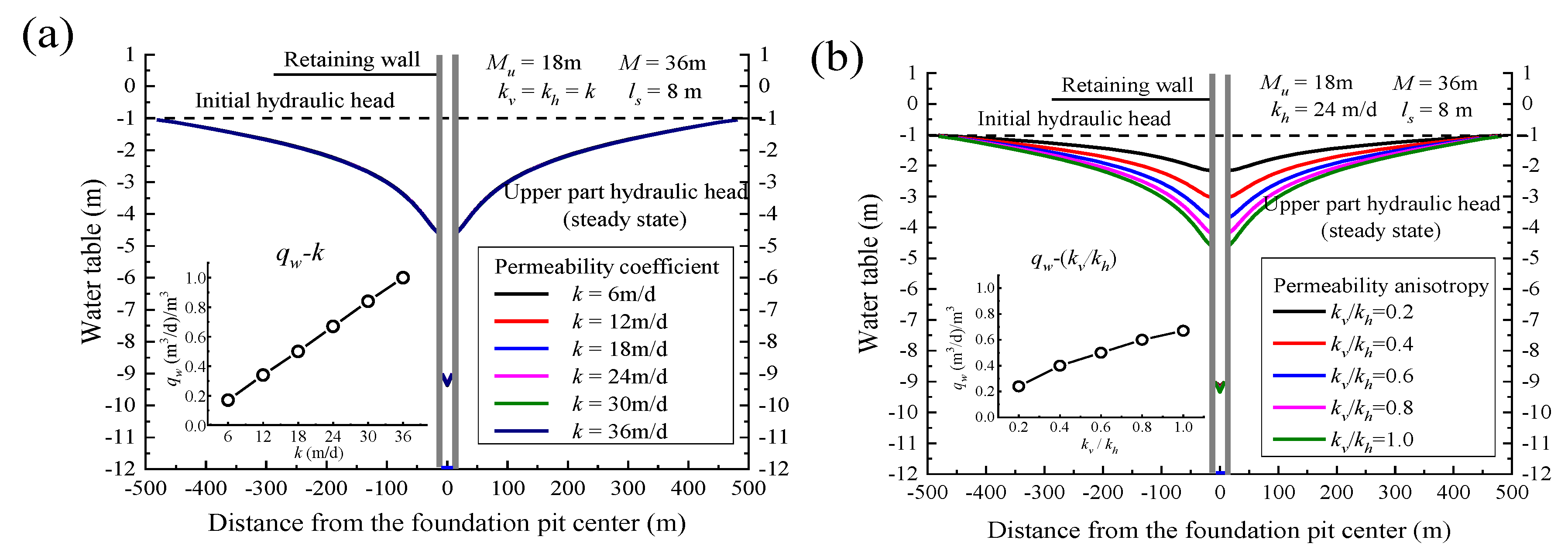
The link between the seepage field distribution and dewatering efficiency is obtained by adjusting Qw until sw reaches 8 m and by changing the dewatering parameters individually within a reasonable range, as shown in Figure 5. The seepage field distribution is reflected by the measured drawdowns, and the improved dewatering efficiency is defined by a less qw ((m3/d)/(m2∙m)), as follows:
(1) Permeability coefficient (k): k is applied to homogeneous aquifers. As shown in Figure 5a, water table remains unchanged when k increases but qw increases linearly. In addition, this coefficient satisfies the linear relationship between k and qw in Darcy’s law. The result indicates that k affects dewatering efficiency only by changing flow velocities instead of the seepage field distribution.
(2) Permeability anisotropy (kv/kh): The sedimentary process forms a thin sticky layer that prevents vertical flow, and seepage velocity varies in different directions [41]; thus, seepage pressure distribution and vertical velocity change. The increasing anisotropy causes qw to decline nonlinearly with rising water table due to an increase in vertical hydraulic gradient and the inevitable detour flow. Consequently, dewatering efficiency is enhanced.
(3) Aquifer thickness (M): Water table rises as M increases, and the Mu/M ratio remains fixed (0.5), while qw also increases. A large hydraulic recharge area and a long flow path are obtained when the 3D seepage field is stretched vertically, enhancing hydraulic recharge and raising the groundwater head to the aquifer top.
(4) Insertion depth of the barrier (Mu): The penetration of curtains generates the blocking effects (i.e., flow direction transfer, flow path lengthening, and seepage area reduction). Water table rises, and qw is reduced gradually when Mu increases. The superposition of the wall–well effect has been proved to affect the distribution of seepage field in simulations; that is, upper-part flows slow down and turn downward, whereas flow velocities below the wall increase [42]. Besides, numerical results in Figure 5d show the minor dewatering effort requirement with the squeezing deformation of wall-bottom seepage field. The phenomena in simulations indicate that the squeezed seepage field produces additional vertical flows and results in substantial energy consumption and enhanced dewatering efficiency. However, flow velocity increases may also bring about erosive phenomena [42].
(5) Pumping well screen length (ls): The design value of ls relies on field conditions, such that a small ls will produce a small qw with the water table maintained outside. Thus, minimal influence is exerted on the seepage field distribution outside with various ls values, but a long flow path is produced inside.
From the analysis of the different seepage characteristics, the effects of the parameters on the seepage field can be summarized as follows: (1) The variation of flow velocities and (2) the deformation of the 3D seepage field. When a single parameter changes, flow velocity (k) or seepage field distribution (M, Mu, ls) changes separately or both factors are influenced (kv/kh); thus, dewatering efficiency is significantly affected.
4. Quantification of Blocking Effects
The wall–well design of the dewatering control scheme must obtain Qw in advance. The formalized inflow prediction formulas are established on the basis of seepage characteristic analysis by quantifying the link between dewatering parameters with Qw.
4.1. Equivalent Pumping Well Inflow
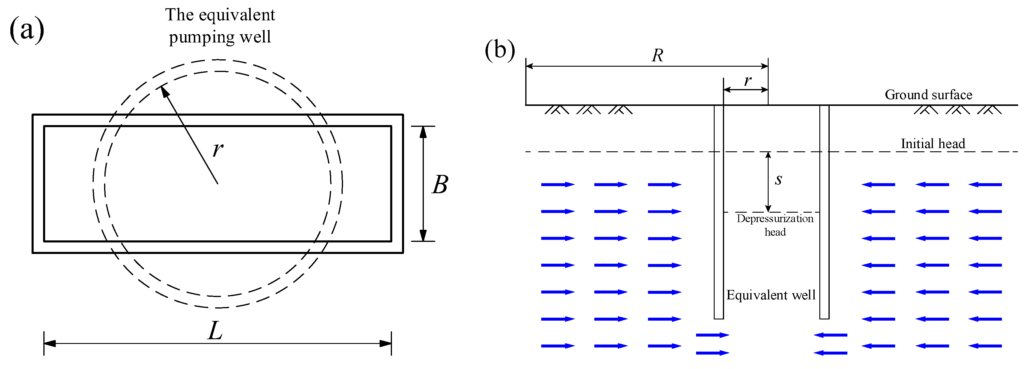
For reference, equivalent inflow QT is proposed under the hypothesis of parallel flow, in which the pit is regarded as a full penetrating pumping well in the absence of 3D flow, as shown in Figure 6.
Then, the following Thiem equation [43] is selected to calculate the QT value of the equivalent pumping well:
where k is the permeability coefficient under Dupuit’s assumption for the equivalent well and inhomogeneous aquifer, k = kh; s is the drawdown inside the equivalent well and is substituted by the average drawdown on the confined aquifer’s top inside the pit, as shown in Figure 6b; r is the inner radius of the equivalent well that can be determined using the formula L × B = 2πr2, as shown in Figure 6a; and T is the transmissivity of the aquifer.
However, Thiem equation reflects the influence of flow velocity (k) but not of seepage field distortion. The parallel flow is transferred to the 3D flow near the curtains and causes seepage field deformation. Thus, the distortion of the 3D seepage field should be quantified.
4.2. 3D Seepage Field Distortion Function
Dewatering under the barriers is divided into four stages [35]—that is, stage I: Groundwater withdrawals only come from aquifers inside pits and drawdown develops with no barrier influence; stage II: Groundwater withdrawals come from aquifers inside and outside pits and drawdown is in influenced by the presence of barriers; stage III: Groundwater withdrawals are supplied by outside aquifer only and drawdown−time curve is parallel to the no barrier condition; stage IV: Pumping reaches the stable state and drawdown becomes constant. On the basis of the empirical dewatering scheme, when t = 100 d, the transient flow enters Stage IV. At this point, it closely approaches the steady state (error <5%). The numerical results of the Qc–s curve are obtained under various conditions by adjusting inflow in the numerical model. The inflow modification factor Qd of the equivalent well with barriers can be calculated under a particular drawdown s as follows:
4.2.1. Normalized Form
To generalize the calculation results, the parameters affecting the seepage field distributions are converted to their normalized form. This form contains the relative barrier ratio bd (Mu/M), non-standard thickness coefficient Md (36/M), permeability anisotropy coefficient kd (kd/kh), and well screen insertion ratio ld (ls/Mu). In the standard state, the normalized parameters are set as kd = 1, ld = 1, and Md = 1 (M = 36 m).
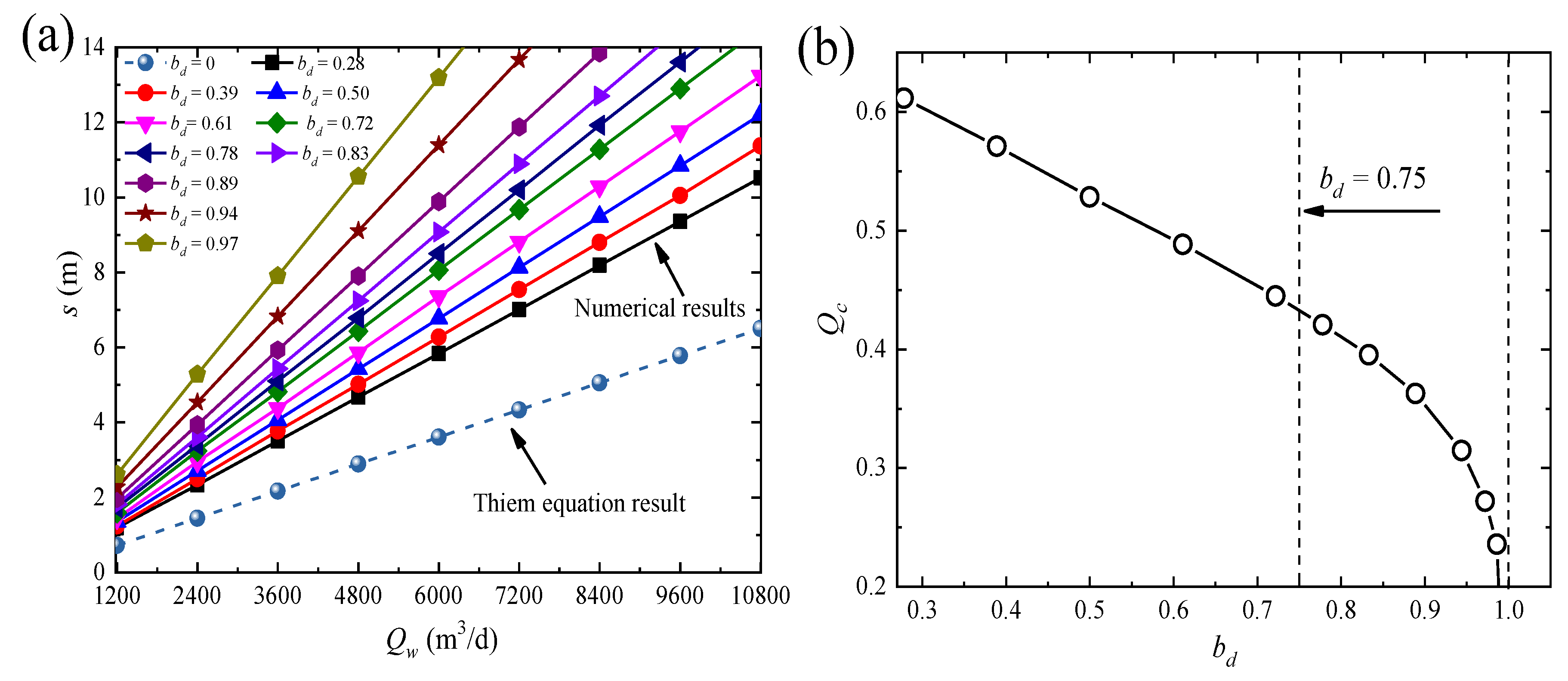
4.2.2. Standard Curve
In the standard state, the numerical results (Qc–s) with different bd and Thiem results (QT–s) can be obtained by specifying an inflow set, as shown in Figure 7a. The resulting curves show the linear distribution but with different slopes. All the slopes of the numerical result curves are greater than that of the Thiem result curve. An increase in bd gradually increases the curve slope of the numerical results. Such increase shows that a large bd will enhance sensitivity between inflow and drawdowns. The Qd–bd curves can be calculated using Equation (8) by setting different s values, and all the curves under different s values converge to a single curve, as shown in Figure 7b. Such convergence indicates that the inflow reduction caused by the 3D flow is uniform under different drawdowns in a particular state. By regarding this converged curve as the standard curve and writing Qd as Qs in this state, a separate nonlinear function of the standard curve can be expressed by artificially defining the line type boundary (bd = 0.75) as follows:
However, this formula can only be applied to the standard state but not to conditions with non-standard parameters (Md, kd, and ld). Thus, additional distortion functions are required.
4.2.3. Distortion Function
(a) Permeability coefficient (k): The Qd–bd curves with different k values are presented in Figure 8a using the same analysis method as that for the standard curve. The results show that all the curves are consistent with those of the standard curve, indicating that k is a non-disturbing factor for the seepage field distribution. Modification is unnecessary because only flow velocity is changed.
(b) Permeability anisotropy coefficient (kd): Similarly, the Qd–bd curves under different kd values are established and shown in Figure 8b. A decrease in kd increases the deviation between Qd and Qs, but linear deviations (the offset value <10%) occur as kd approaches 0.2 and below. By disregarding this linear deviation and modifying Qs to Qd under the corresponding kd, the distortion function of permeability anisotropy is constructed as follows:
(c) Non-standard thickness coefficient (Md): Figure 8c presents the Qd–bd curves under different Md values. The figure shows that the Qd–bd curves diverge as Md changes with a similar line type. When Md > 1, the curve moves upward; otherwise, it shifts downward. By quantifying the variation of the standard curve, the distortion function of aquifer thickness is given as:
(d) Well screen insertion ratio (ld): To utilize the wall–well effects, a short screen length is provided in the field to lengthen flow path. The Qd–bd curves at different ld values are shown in Figure 8d. The line type of the curves remains, but the curves move downward with decreasing ld values. The variation can be quantified using the following distortion function of screen length:
4.2.4. Inflow Prediction with Partial Penetrating Curtains
To increase the similarity between inflow prediction and actual conditions, Qs can be approximately modified to Qd by multiplying it to the normalized distortion function as follows:
Furthermore, the empirical inflow prediction formula of the overall station pit that is suitable for the sand and gravel strata (i.e., MAS) with high permeability is established as follows:
Combined with Equations (13) and (14), the inflow of steady flow can be effectively calculated using the formalized equations with the determined predesign parameters.
5. Field Application
5.1. Design Method of the Dewatering Scheme
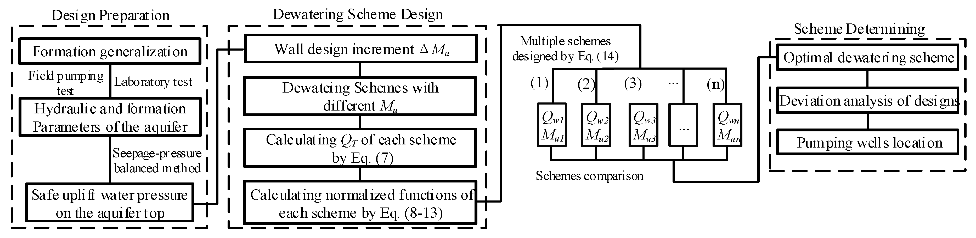
On the basis of the preceding empirical prediction equations, the design method of the dewatering scheme with barriers in the sand and gravel strata is presented in Figure 9, where the increment in ∆Mu is determined through design precision and hydraulic conditions.
5.2. Dewatering Design of the Shuibu Metro Station
5.2.1. Hydrogeological Conditions of the Area
The dewatering scheme combining partial penetrating curtains and wells is selected for groundwater control during the excavation of this case. The hydrogeological conditions of the area are presented in Figure 10. Possible connection regions in the silty clay layers are blocked via grouting to reduce hydraulic recharge from the aquifers. Then, the strata are generalized again during the design period, as shown in Figure 11. Before curtain construction, field pumping and laboratory tests are conducted to obtain permeability in various directions as follows: kh = 24.5 m/d and kv = 15 m/d.
5.2.2. Depressurization Requirements
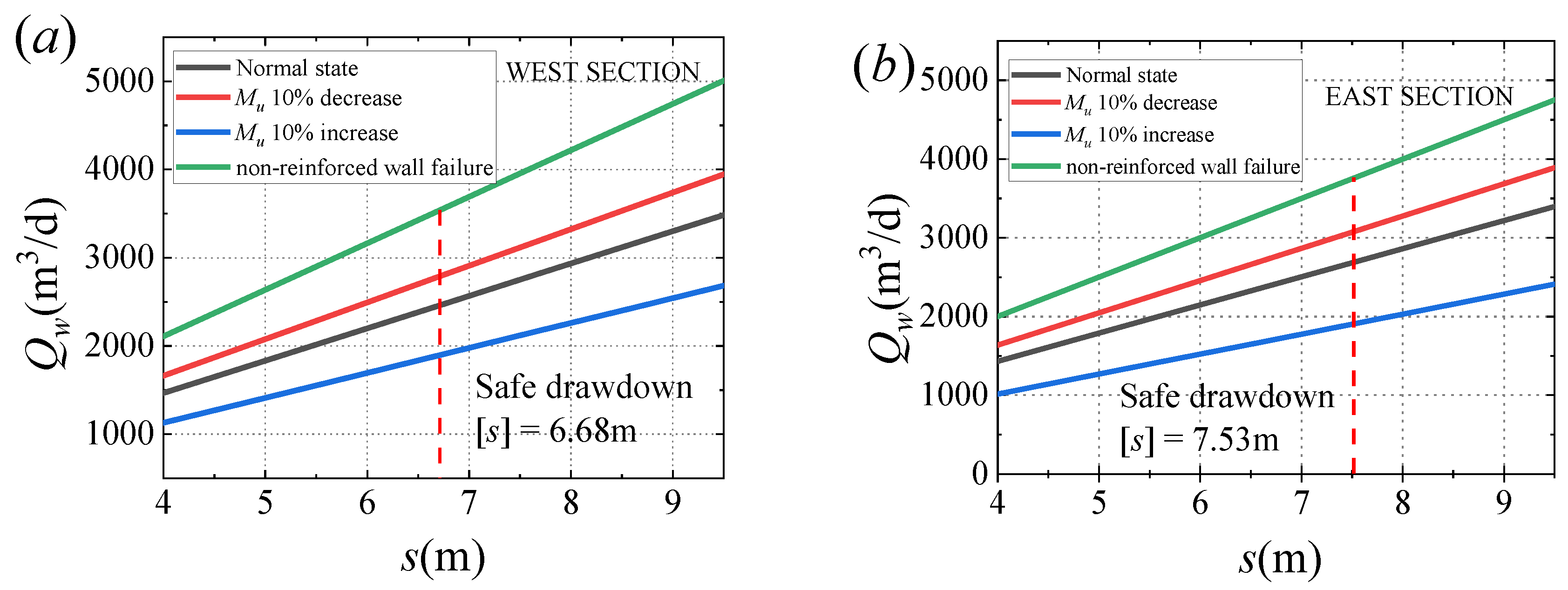
The depressurization requirements of uplift pressure can be calculated using the classic soil–pressure balanced method [33]. The calculated safe drawdown (s) of the west and east sections is 6.68 m and 7.53 m, respectively.
5.2.3. Dewatering Scheme Design
The designed length of the reinforced diaphragm wall for load bearing is 31.5 m in engineering applications. For groundwater blocking, non-reinforced concrete curtains should be added at the wall’s bottom. The multiple schemes and corresponding inflow are determined as follows. (a) On the basis of ∆Mu (2 m), as set by construction organizations, various alternative schemes with different Mu (integers) are presented in Figure 11. (b) The short well screen (ls = Mu/3) is selected to enhance the wall–well effect. (c) R is set as 330 m (west) and 370 m (east) on the basis of the field pumping tests and Equation (5). (d) QT is calculated using Equation (7) with a value of 4328 m3/d (west) and 5187 m3/d (east). (e) The distortion functions (normalized) and inflow of each scheme are presented in Table 3 and Figure 12, respectively.
5.2.4. Comparison of Dewatering Control Schemes
Completely blocking seepage using the 12.5 m non-reinforced concrete curtain is impossible due to the layer fluctuations and dispersions of aquitards. The inevitable partial blocking leads to an uncertain inflow with large errors. Moreover, the microflow with a large flow velocity poses a risk of formation damage. The water pressure difference of curtains is difficult to release without sufficient groundwater flow and may cause leakage at vulnerable points of the curtains. Therefore, a scheme of 10.5 m non-reinforced concrete curtain with a controllable prediction Qw of 2450 m3/d (west) and 2694 m3/d (east) is selected.
5.2.5. Deviation Control Curves
Two types of design deviations are proposed by considering field conditions. (a) The layer fluctuation may cause changes in the actual Mu, and 10% deviations are set in this study. (b) The partial failure of non-reinforced concrete curtains changes the blocking effects, and curtains with half-part failure (5 m) are assumed to be the limit state. Hence, deviation control curves are calculated using the inflow prediction formulas shown in Figure 13. On this basis, three levels of dewatering system states are presented: Wall-failure, layer-fluctuation, and normal states. The upper limits of the deviation control curves are presented in Figure 13. Cautious schemes are then adopted on the basis of the crossover points of the deviation control curves and safe drawdown lines. In this project, the corresponding control inflow is 3600, 3000, and 2400 m3/d under safe drawdowns.
5.2.6. Location of Pumping Wells
Pumping wells are located in accordance with the control inflow of the three level states. As shown in Figure 14, four pumping wells (Y: 600 m3/d) are located inside each section of the pit to ensure its construction safety under normal state (2400 m3/d). For the wall-failure state, two reserved pumping and observation wells (G: 600 m3/d) are added (total of 3600 m3/d). Given the high porosity and compressibility of the silty sand layer, observation wells (SW) outside the pit are installed to observe head changes in the silty sand layer with high external sensitivity.
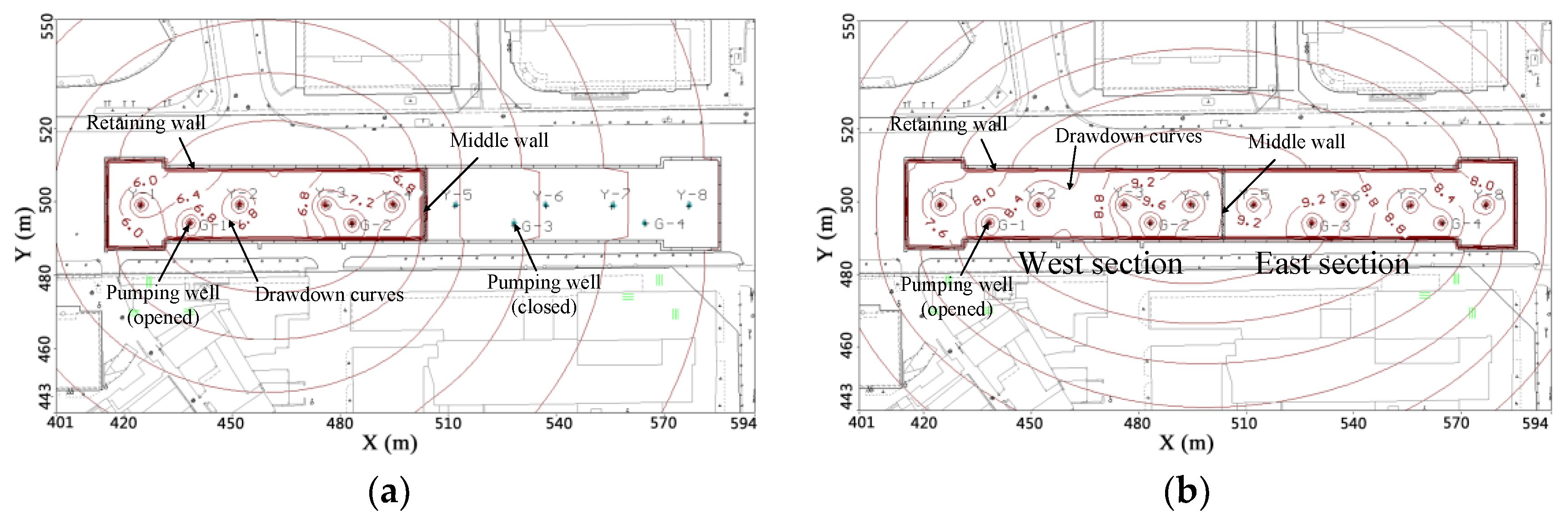
A numerical model was performed to check the effectiveness of the designed dewatering system. Considering the possible adverse conditions caused by the wall construction defects, the failure and leaking of 6 m non-reinforced bottom wall was taken into consideration in the numerical model. The simulation of two-stage dewatering with wall-failure state was conducted according to the actual excavation sequences (west to east), as presented in Figure 15. The numerical results show the calculated average drawdown (6.8 m) was almost consistent with prediction results during dewatering inside the west-subsection excavation. With the development of the subsequent dewatering inside east-subsection excavation, all the wells were gradually activated. The excessive drawdowns were caused by dewatering inside the two subsection excavations, which may induce large settlements outside. Thus, the control of both the amount of pumping wells and dewatering time needs to be carried out during the actual excavation dewatering.
5.3. Field Verification
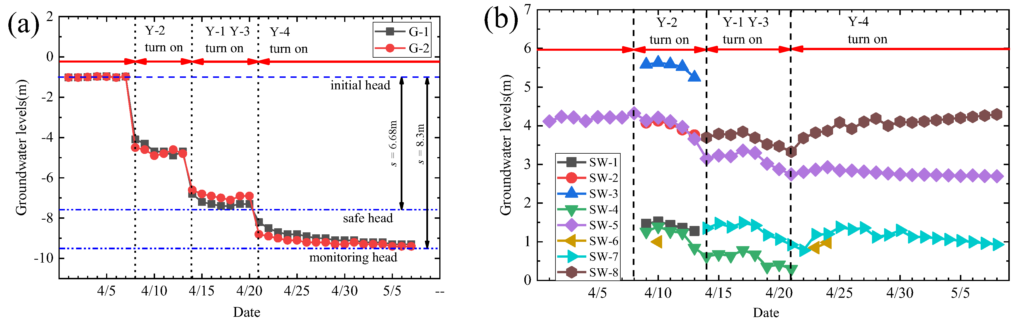
The observation data inside the west section are gathered for analysis due to the impervious dewatering process, the inflow and corresponding head variations are shown in Figure 16. With the pumping wells successively turning on, the uplift head inside the west section exhibits a segmented downward trend during pumping, as shown in Figure 16a, and displays evident depressurization effect. Meanwhile, the measured heads at (G-1) and (G-2) are approximately uniform throughout the entire dewatering process. Thus, introducing the average drawdown s inside is reasonable. When seepage approaches a steady state, s finally reaches 8.3 m with an inflow of 2400 m3/d (four wells) to ensure the stability of the pit bottom. The dewatering system is within the range of the normal state curve and the (Mu + 10%) deviation control curve shown in Figure 13a. Hence, a 25% design safe margin is set for the west section dewatering design. For the head variations in the upper aquitard outside the pit, Figure 16b shows the measured data during pumping. Drawdowns are around 1 m and 0.5 m near the west and east sides, respectively. These findings satisfy the control value (2 m) required by construction safety. Moreover, several heads outside return to their initial states due to the powerful recharge of aquifers. The constant stability of the excavation surface in the entire construction process verifies the reliability of the design method.
6. Discussion
Partially penetrating curtains in the seepage field generate considerable head differences between the outside and inside of the aquifer. Such differences indicate that the 3D seepage field formed by the wall–well effects plays an important role in groundwater control during excavation. Drawdowns are concentrated in the aquifer bottom and the curtain-enclosing scopes because of the vertical flow anisotropy of the aquifer. The distribution induces the water pressure to satisfy the uplift pressure requirement outside and the decompression requirement inside. Furthermore, water pressure differences are reduced at the bottom of curtains to prevent damages and leaks. Thus, the 3D flow enables the appropriate distribution of the pressure head in dewatering construction.
However, an empirical prediction may not completely fit the observation data. The following simplified hypotheses should be further discussed in establishing inflow formulas that result in uncertain deviations between predictions and reality.
- A quantitative analysis is based on the assumption that aquifer permeability is uniformly distributed at each point in the influence domain. However, many deep structures (e.g., pile foundations and high-rise building basements) have dispersed clay and grouting structures around the pumping influence area; this condition reduces the regional permeability of aquifers [35]. When these obstructions are located in regions with dense flows (e.g., foundation pit scope and curtain bottom), dewatering efficiency is substantially improved due to flow blocking.
- Non-Darcy flow occurs with a fast flow velocity [34] that is evident at the wall bottom and near the pumping well. Moreover, the wall–well effects enhance the non-Darcy flow effect and further promote dewatering efficiency.
- The parameter coupling effect is not considered in formula establishment. For example, when kd decreases and the other parameters vary to extend the vertical flow path, groundwater control efficiency may be improved rather than the multiplication of distortion functions caused by the separate variation of parameters.
Thus, the aforementioned cumulative effects lead to conservative prediction values. Consequently, the measured drawdowns are nearly 1.6 m higher than the prediction in the field. However, detecting a particular distribution of the overall strata at limited cost is nearly impossible using existing technologies. Moreover, the exact range of non-Darcy flow is uncertain because of the unclear boundaries of the nonlinear laminar and the laminar [36]. Hence, quantifying the non-Darcy flow effect is difficult. For the algorithm that considers multi-parameter coupling, a complex algorithm is inappropriate for field application. To ensure safety, the preceding simplified hypotheses are applied to field dewatering design, in which they are reasonable and provide safe construction conditions within engineering accuracy.
7. Conclusions
This study presents a formalized inflow formula for pits with partial penetrating curtains based on seepage characteristic analysis. The corresponding design method is further developed for the dewatering scheme design in sand and gravel strata and applied to a field case for verification. The following conclusions are drawn.
- FDM is adopted to analyze dewatering seepage characteristics with curtains. The results show that the seepage field with various parameters exhibits different distributions and flow velocities that affect steady inflow Qw. Among the parameters, k plays a key role in flow velocity. Meanwhile, the other parameters, such as kv/kh, M, Mu, and ls, change the seepage field distribution.
- Inflow prediction formulas for pits with partial penetrating curtains in high-permeability aquifers are proposed under the assumption of an equivalent well by establishing the function of the Qd–bd curve and quantifying seepage deformation.
- A design method for dewatering schemes is proposed and applied to the dewatering design of the Shuibu Metro Station. The scheme of a 31.5 m reinforced concrete diaphragm wall combined with a 10.5 m non-reinforced concrete wall is adopted. Considering the design deviation of the formation generalization and curtain leakage, four main pumping wells combined with two reserved pumping wells are located in each subsection of the excavation for groundwater control. This design scheme maintains a safe margin of 25%, and the external drawdown is controlled within 1 m in the field to ensure safety during inside and outside excavations.
Author Contributions
Conceptualization, L.L.; investigation, L.L.; methodology, C.C.; resources, C.S.; writing—original draft, L.L.; writing—review and editing, M.L.
Funding
Projects funded by the National Natural Science Foundation of China (No. 51978669, U1734208), the Natural Science Foundation of Hunan Province, China (No. 2018JJ3657), and the Fundamental Research Funds for the Central Universities of Central South University (No. 2019zzts294) are gratefully acknowledged.
Acknowledgments
The authors are grateful for the funds provided by Guangzhou Metro Design & Research Institute Co., Ltd. and CCCC Strait Construction Investment and Development Co., Ltd. The authors also thank the 2nd Harbor Engineering Co., Ltd., of CCCC for cooperation in the field tests and data collection for this study.
Conflicts of Interest
The authors declare no conflict of interest.
References
- Lei, M.; Lin, D.; Huang, Q.; Shi, C.; Huang, L. Research on the construction risk control technology of shield tunnel underneath an operational railway in sand pebble formation: A case study. Eur. J. Environ. Civ. Eng. 2018, 22, 1–15. [Google Scholar] [CrossRef]
- Luo, Z.J.; Zhang, Y.Y.; Wu, Y.X. Finite element numerical simulation of three-dimensional seepage control for deep foundation pit dewatering. J. Hydrodyn. 2008, 20, 596–602. [Google Scholar] [CrossRef]
- Xu, Y.S.; Ma, L.; Du, Y.J.; Shen, S.L. Analysis of urbanisation-induced land subsidence in Shanghai. Nat. Hazards 2012, 63, 1255–1267. [Google Scholar] [CrossRef]
- Xu, Y.S.; Wu, H.N.; Wang, B.Z.F.; Yang, T.L. Dewatering induced subsidence during excavation in a Shanghai soft deposit. Environ. Earth Sci. 2017, 76. [Google Scholar] [CrossRef]
- Lei, M.; Liu, J.; Lin, Y.; Shi, C.; Liu, C. Deformation Characteristics and Influence Factors of a Shallow Tunnel Excavated in Soft Clay with High Plasticity. Adv. Civ. Eng. 2019, 2019, 7483628. [Google Scholar] [CrossRef]
- Xu, Y.S.; Shen, J.S.; Zhou, A.N.; Arulrajah, A. Geological and hydrogeological environment with geohazards during underground construction in Hangzhou: A review. Arab. J. Geosci. 2018, 11, 544. [Google Scholar] [CrossRef]
- Wu, Y.X.; Lyu, H.M.; Han, J.; Shen, S.L. Dewatering-induced building settlement around a deep excavation in soft deposit in Tianjin, China. J. Geotech. Geoenviron. Eng. 2019, 145, 5019003. [Google Scholar] [CrossRef]
- Shen, S.L.; Wu, Y.X.; Xu, Y.S.; Hino, T.; Wu, H.N. Evaluation of hydraulic parameters from pumping tests in multi-aquifers with vertical leakage in Tianjin. Comput. Geotech. 2015, 68, 196–207. [Google Scholar] [CrossRef]
- Wang, Y.; Jiao, J.J. Origin of groundwater salinity and hydrogeochemical processes in the confined Quaternary aquifer of the Pearl River Delta, China. J. Hydrol. 2012, 438–439, 112–124. [Google Scholar] [CrossRef]
- Cao, C.; Shi, C.; Lei, M. A simplified approach to design jet-grouted bottom sealing barriers for deep excavations in deep aquifers. Appl. Sci. 2019, 9, 2307. [Google Scholar] [CrossRef]
- Cao, C.; Shi, C.; Liu, L.; Liu, J.; Lei, M.; Lin, Y.; Ye, Y. Novel excavation and construction method for a deep shaft excavation in Ultrathick aquifers. Adv. Civ. Eng. 2019, 2019, 1827479. [Google Scholar] [CrossRef]
- Jurado, A.; De Gaspari, F.; Vilarrasa, V.; Bolster, D.; Sánchez-Vila, X.; Fernàndez-Garcia, D.; Tartakovsky, D.M. Probabilistic analysis of groundwater-related risks at subsurface excavation sites. Eng. Geol. 2012, 125, 35–44. [Google Scholar] [CrossRef]
- Huang, Y.; Bao, Y.; Wang, Y. Analysis of geoenvironmental hazards in urban underground space development in Shanghai. Nat. Hazards 2014, 75, 2067–2079. [Google Scholar] [CrossRef]
- Shi, C.; Cao, C.; Lei, M.; Peng, L.; Jiang, J. Optimal design and dynamic control of construction dewatering with the consideration of dewatering process. KSCE J. Civ. Eng. 2017, 21, 1161–1169. [Google Scholar] [CrossRef]
- Roy, D.; Robinson, K.E. Surface settlements at a soft soil site due to bedrock dewatering. Eng. Geol. 2009, 107, 109–117. [Google Scholar] [CrossRef]
- Pujades, E.; Vàzquez-Suñé, E.; Carrera, J.; Jurado, A. Dewatering of a deep excavation undertaken in a layered soil. Eng. Geol. 2014, 178, 15–27. [Google Scholar] [CrossRef]
- Pujades, E.; Vázquez-Suñé, E.; Carrera, J.; Vilarrasa, V.; De Simone, S.; Jurado, A.; Ledesma, A.; Ramos, G.; Lloret, A. Deep enclosures versus pumping to reduce settlements during shaft excavations. Eng. Geol. 2014, 169, 100–111. [Google Scholar] [CrossRef]
- Wu, Y.X.; Shen, S.L.; Wu, H.N.; Xu, Y.S.; Yin, Z.Y.; Sun, W.J. Environmental protection using dewatering technology in a deep confined aquifer beneath a shallow aquifer. Eng. Geol. 2015, 196, 59–70. [Google Scholar] [CrossRef]
- Pujades, E.; De Simone, S.; Carrera, J.; Vázquez-Suñé, E.; Jurado, A. Settlements around pumping wells: Analysis of influential factors and a simple calculation procedure. J. Hydrol. 2017, 548, 225–236. [Google Scholar] [CrossRef]
- Shen, S.L.; Han, J.; Du, Y.J. Deep mixing induced property changes in surrounding sensitive marine clays. J. Geotech. Geoenviron. Eng. 2008, 134, 845–854. [Google Scholar] [CrossRef]
- Chen, J.J.; Zhang, L.; Zhang, J.F.; Zhu, Y.F.; Wang, J.H. Field tests, modification, and application of deep soil mixing method in soft clay. J. Geotech. Geoenviron. Eng. 2013, 139, 24–34. [Google Scholar] [CrossRef]
- Shen, S.L.; Wang, Z.F.; Horpibulsuk, S.; Kim, Y.H. Jet grouting with a newly developed technology: The Twin-Jet method. Eng. Geol. 2013, 152, 87–95. [Google Scholar] [CrossRef]
- Wang, Z.F.; Shen, S.L.; Ho, C.E.; Kim, Y.H. Investigation of field-installation effects of horizontal twin-jet grouting in Shanghai soft soil deposits. Can. Geotech. J. 2013, 50, 288–297. [Google Scholar] [CrossRef]
- Xu, Y.S.; Shen, S.L.; Ma, L.; Sun, W.J.; Yin, Z.Y. Evaluation of the blocking effect of retaining walls on groundwater seepage in aquifers with different insertion depths. Eng. Geol. 2014, 183, 254–264. [Google Scholar] [CrossRef]
- Vilarrasa, V.; Carrera, J.; Jurado, A.; Pujades, E.; Vázquez-Suné, E. A methodology for characterizing the hydraulic effectiveness of an annular low-permeability barrier. Eng. Geol. 2011, 120, 68–80. [Google Scholar] [CrossRef]
- Pujades, E.; Jurado, A.; Carrera, J.; Vázquez-Suñé, E.; Dassargues, A. Hydrogeological assessment of non-linear underground enclosures. Eng. Geol. 2016, 207, 91–102. [Google Scholar] [CrossRef]
- Pujades, E.; López, A.; Carrera, J.; Vázquez-Suñé, E.; Jurado, A. Barrier effect of underground structures on aquifers. Eng. Geol. 2012, 144–145, 41–49. [Google Scholar] [CrossRef]
- Wu, Y.X.; Shen, S.L.; Xu, Y.S.; Yin, Z.Y. Characteristics of groundwater seepage with cut-off wall in gravel aquifer. I: Field observations. Can. Geotech. J. 2015, 52, 1526–1538. [Google Scholar] [CrossRef]
- Wu, Y.X.; Shen, S.L.; Yin, Z.Y.; Xu, Y.S. Characteristics of groundwater seepage with cut-off wall in gravel aquifer. II: Numerical analysis. Can. Geotech. J. 2015, 52, 1539–1549. [Google Scholar] [CrossRef]
- Wu, Y.X.; Shen, J.S.; Cheng, W.C.; Hino, T. Semi-analytical solution to pumping test data with barrier, wellbore storage, and partial penetration effects. Eng. Geol. 2017, 226, 44–51. [Google Scholar] [CrossRef]
- Shen, S.L.; Wu, Y.X.; Misra, A. Calculation of head difference at two sides of a cut-off barrier during excavation dewatering. Comput. Geotech. 2017, 91, 192–202. [Google Scholar] [CrossRef]
- Zhou, N.; Vermeer, P.A.; Lou, R.; Tang, Y.; Jiang, S. Numerical simulation of deep foundation pit dewatering and optimization of controlling land subsidence. Eng. Geol. 2010, 114, 251–260. [Google Scholar] [CrossRef]
- Wang, J.; Feng, B.; Guo, T.; Wu, L.; Lou, R.; Zhou, Z. Using partial penetrating wells and curtains to lower the water level of confined aquifer of gravel. Eng. Geol. 2013, 161, 16–25. [Google Scholar] [CrossRef]
- Wang, J.; Liu, X.; Wu, Y.; Liu, S.; Wu, L.; Lou, R.; Lu, J.; Yin, Y. Field experiment and numerical simulation of coupling non-Darcy flow caused by curtain and pumping well in foundation pit dewatering. J. Hydrol. 2017, 549, 277–293. [Google Scholar] [CrossRef]
- Wu, Y.X.; Shen, S.L.; Yuan, D.J. Characteristics of dewatering induced drawdown curve under blocking effect of retaining wall in aquifer. J. Hydrol. 2016, 539, 554–566. [Google Scholar] [CrossRef]
- Wang, J.; Liu, X.; Liu, S.; Zhu, Y.; Pan, W.; Zhou, J. Physical model test of transparent soil on coupling effect of cut-off wall and pumping wells during foundation pit dewatering. Acta Geotech. 2019, 14, 141–162. [Google Scholar] [CrossRef]
- Xu, Y.S.; Yan, X.X.; Shen, S.L.; Zhou, A.N. Experimental investigation on the blocking of groundwater seepage from a waterproof curtain during pumped dewatering in an excavation. Hydrogeol. J. 2019, 27, 1–14. [Google Scholar] [CrossRef]
- Bear, J. Hydraulics of Groundwater; McGraw-Hill: New York, NY, USA, 2012. [Google Scholar]
- McDonald, M.G.; Harbaugh, A.W. A Modular Three-Dimensional Finite-Difference Groundwater Flow Model; US Geological Survey: Reston, VA, USA, 1984.
- Harbaugh, B.A.W.; Banta, E.R.; Hill, M.C.; Mcdonald, M.G. MODFLOW-2000, The U.S. Geological Survey Modular Graound-Water Model—User Guide to Modularization Concepts and the Ground-Water Flow Process; U.S. Geological Survey: Reston, VA, USA, 2000; Volumn 130.
- Wilson, A.M.; Huettel, M.; Klein, S. Grain size and depositional environment as predictors of permeability in coastal marine sands. Estuar. Coast. Shelf Sci. 2008, 80, 193–199. [Google Scholar] [CrossRef]
- Colombo, L.; Gattinoni, P.; Scesi, L. Influence of underground structures and infrastructures on the groundwater level in the urban area of Milan. Int. J. Sustain. Dev. Plann. 2017, 12, 176–184. [Google Scholar] [CrossRef]
- Thiem, G. Hydrologische Methoden; Gebhardt: Leipzig, Germany, 1906. [Google Scholar]
Figure 1.
(a) Geographical location of the study site. (b) Plan view of the foundation pit.

Figure 2.
Geological profile of the Shuibu Metro Station.

Figure 3.
Problem sketch: (a) plan view of the rectangle excavation pit; (b) cross-section view of barriers and aquifers. Note: Qw = pumping rate of wells; L = inner length of the retaining wall; B = inner width of the retaining wall; M = thickness of the confined aquifer; Mu = insertion depth of the barrier; Mn = distance from bottom of barrier to the lower aquitard; ls = screen length.

Figure 4.
Finite difference mesh: (a) Three-dimensional (3D) view of the mesh; (b) plan view of the mesh around the pit; (c) central cross-section of the mesh.
Figure 4.
Finite difference mesh: (a) Three-dimensional (3D) view of the mesh; (b) plan view of the mesh around the pit; (c) central cross-section of the mesh.


Figure 5.
Water table on the central cross-section with variation dewatering parameters: (a) Permeability; (b) permeability anisotropy; (c) aquifer thickness; (d) insertion depth of barriers; (e) screen length of pumping well.
Figure 5.
Water table on the central cross-section with variation dewatering parameters: (a) Permeability; (b) permeability anisotropy; (c) aquifer thickness; (d) insertion depth of barriers; (e) screen length of pumping well.


Figure 6.
The equivalent pumping well: (a) Cross-section; (b) vertical section.

Figure 7.
Variation results in the standard state: (a) Qw–s curve with different bd; (b) standard curve.
Figure 7.
Variation results in the standard state: (a) Qw–s curve with different bd; (b) standard curve.

Figure 8.
Variation curve of Qd–bd with varying dewatering parameters: (a) Permeability coefficient; (b) permeability anisotropy coefficient; (c) non-standard thickness coefficient; (d) well screen insertion ratio.
Figure 8.
Variation curve of Qd–bd with varying dewatering parameters: (a) Permeability coefficient; (b) permeability anisotropy coefficient; (c) non-standard thickness coefficient; (d) well screen insertion ratio.

Figure 9.
Dewatering scheme design method with partial penetrating curtains.

Figure 10.
Hydrogeological conditions of the area: (a) Hydrogeological map of Fuzhou basin and coastal plain; (b) hydrogeological profile of the metro line.
Figure 10.
Hydrogeological conditions of the area: (a) Hydrogeological map of Fuzhou basin and coastal plain; (b) hydrogeological profile of the metro line.

Figure 11.
Strata generalization and designed curtain schemes.

Figure 12.
Pumping rate prediction of various schemes.

Figure 13.
Deviation control curves: (a) West section; (b) east section.

Figure 14.
Location of the wells.

Figure 15.
Numerical simulation of the dewatering system: (a) West section dewatering; (b) overall pit dewatering.
Figure 15.
Numerical simulation of the dewatering system: (a) West section dewatering; (b) overall pit dewatering.

Figure 16.
Groundwater level variation during excavation: (a) Aquifer top within the pit; (b) upper aquitard outside the pit.
Figure 16.
Groundwater level variation during excavation: (a) Aquifer top within the pit; (b) upper aquitard outside the pit.


Table 1.
Hydraulic parameters in geological exploration data.
| Layer | Soil Layer | Type | Thickness (m) | kh (m/d) | kv (m/d) | Ss (1/m) | e | rw (kN/m3) |
|---|---|---|---|---|---|---|---|---|
| I and II | Fill and block stone | Phreatic aquifer | 4.0~6.0 | 8.64 | 8.64 | - | - | 18.5 |
| III | Silt | Upper aquitard | 8.0~12.0 | 0.0055 | 0.0015 | 5 × 10⁻⁴ | 1.67 | 15.7 |
| IV | Silt with sand | Upper aquitard | 10.0~12.0 | 0.54 | 0.3 | 5 × 10⁻⁴ | - | 16.2 |
| V | Sand | Confined aquifer | 16.0~18.0 | 24 (Isotropy) | 2 × 10⁻⁴ | 1.50 | 19.0 | |
| VI | Silty clay (dispersive) | Aquitard (partial) | 0.0~6.0 | 0.003 | 0.002 | 5 × 10⁻⁴ | 0.71 | 19.5 |
| VII | Gravel | Confined aquifer | 4.0~6.0 | 40 | 40 | - | - | 17.0 |
| IV | Granite | Aquitard | Bottom | - | - | - | - | 21.0 |
Table 2.
Simplified parameters in the calculation model.
| No. | Soil Layer | M (m) | kh (m/d) | kv (m/d) | Ss (1/m) |
|---|---|---|---|---|---|
| 1 | Phreatic aquifer | 6 | 8.64 | 8.64 | - |
| 2 | Aquitard | 18 | 0.005 | 0.001 | 5 × 10⁻⁴ |
| 3 | Confined aquifer | 36 | 24 | 24 | 2 × 10⁻⁴ |
Table 3.
Normalized seepage field distortion function.
| Section | Lp | Qs | α | β | η | Qd | Section | Lp | Qs | α | β | η | Qd |
|---|---|---|---|---|---|---|---|---|---|---|---|---|---|
| West | 0 | 0.634 | 0.76 | 1.60 | 1.18 | 0.916 | East | 0 | 0.601 | 0.76 | 1.52 | 1.02 | 0.711 |
| 2.5 | 0.575 | 0.76 | 1.60 | 0.99 | 0.699 | 2.5 | 0.549 | 0.76 | 1.52 | 0.94 | 0.598 | ||
| 4.5 | 0.529 | 0.76 | 1.60 | 0.94 | 0.604 | 4.5 | 0.507 | 0.76 | 1.52 | 0.90 | 0.533 | ||
| 6.5 | 0.482 | 0.76 | 1.60 | 0.90 | 0.531 | 6.5 | 0.466 | 0.76 | 1.52 | 0.88 | 0.478 | ||
| 8.5 | 0.435 | 0.76 | 1.60 | 0.88 | 0.468 | 8.5 | 0.424 | 0.76 | 1.52 | 0.87 | 0.427 | ||
| 10.5 | 0.372 | 0.76 | 1.60 | 0.87 | 0.393 | 10.5 | 0.363 | 0.76 | 1.52 | 0.86 | 0.361 | ||
| 12.5 | 0 | 0.76 | 1.60 | 0.86 | 0 | 12.5 | 0 | 0.76 | 1.52 | 0.85 | 0 |
© 2019 by the authors. Licensee MDPI, Basel, Switzerland. This article is an open access article distributed under the terms and conditions of the Creative Commons Attribution (CC BY) license (http://creativecommons.org/licenses/by/4.0/).
Share and Cite
MDPI and ACS Style
Liu, L.; Lei, M.; Cao, C.; Shi, C. Dewatering Characteristics and Inflow Prediction of Deep Foundation Pits with Partial Penetrating Curtains in Sand and Gravel Strata. Water 2019, 11, 2182. https://doi.org/10.3390/w11102182
AMA Style
Liu L, Lei M, Cao C, Shi C. Dewatering Characteristics and Inflow Prediction of Deep Foundation Pits with Partial Penetrating Curtains in Sand and Gravel Strata. Water. 2019; 11(10):2182. https://doi.org/10.3390/w11102182
Chicago/Turabian StyleLiu, Linghui, Mingfeng Lei, Chengyong Cao, and Chenghua Shi. 2019. "Dewatering Characteristics and Inflow Prediction of Deep Foundation Pits with Partial Penetrating Curtains in Sand and Gravel Strata" Water 11, no. 10: 2182. https://doi.org/10.3390/w11102182
Note that from the first issue of 2016, this journal uses article numbers instead of page numbers. See further details here.