Article

Addressing Long-Term Operational Risk Management in Port Docks under Climate Change Scenarios—A Spanish Case Study

by
Álvaro Campos
1,*,
José María García-Valdecasas
2,
Rafael Molina
1,
Carmen Castillo
3,
Enrique Álvarez-Fanjul
2 and
Joanna Staneva
4
1
ETSI de Caminos, Canales y Puertos, Universidad Politécnica de Madrid (UPM), HRL-UPM & CEHINAV-UPM, 28040 Madrid, Spain
2
Organismo Público de Puertos del Estado (OPPE), 28042 Madrid, Spain
3
ETSI de Caminos, Canales y Puertos, Universidad de Castilla-La Mancha (UCLM), 13071 Ciudad Real, Spain
4
Helmholtz-Zentrum Geesthacht (HZG), 21502 Geesthacht, Germany
*
Author to whom correspondence should be addressed.
Water 2019, 11(10), 2153; https://doi.org/10.3390/w11102153
Submission received: 13 September 2019 / Revised: 10 October 2019 / Accepted: 11 October 2019 / Published: 16 October 2019
(This article belongs to the Special Issue Effect of Climate Change on Coastal Hydrodynamics)

Abstract

:
Ports are strategic hubs of the logistic chain and are likely to be exposed to natural hazard events. Variation of metocean agents derived from climate change, such as sea level rise or changes in the magnitude, frequency, duration, and direction of storms, can modify the infrastructural and operational vulnerability of port areas and activities, demanding the development of adaptation or mitigation strategies. In this context, the present paper is aimed to propose a downscaling methodology for addressing local effects at port scale. In addition, based on previously identifying and defining the Areas of Operational Interest (AOIs) inside ports, an approach towards the evaluation of operational vulnerability is offered. The whole process is applied, as a practical case, to the Port of Gijón (Spain) for different General Circulation Models (GCMs), concentration scenarios, and time horizons. The results highlight, in line with other publications, that inter-model differences are, so far, more significant than intra-model differences from dissimilar time horizons or concentration scenarios.

1. Introduction

Presently, most of the world’s freight is moved by sea and, consequently, ports represent one of the most strategic infrastructures in the logistic chain. The economy of scale has pushed towards larger vessels demanding deeper sheltered areas for their operations, increasing their exposition to metocean agents. Most ports regularly experience natural hazard events and their vulnerability might not only be seen from a local or regional point of view but from a global perspective in terms of logistics and trade-dependent industries. In this context, sea level rise and changes in the magnitude, frequency, duration, and direction of storms due to climate change are likely to modify wave-structure interactions patterns and agitation conditions inside ports or, in other words, to alter their infrastructural and operational vulnerability. Addressing this issue is, therefore, of high relevance and can be regarded as a four-step process:
  • Identification and prediction of metocean variables at global level for different climate change scenarios.
  • Downscaling predictions to local high-resolution level inside port areas.
  • Vulnerability analysis (or risk analysis when including costs) of infrastructures and port activities.
  • Development of action plans based on adaptation or mitigation strategies.
The first step is the most addressed so far, with several working groups pushing worldwide for a better understanding of the possible trends, regularly updated in the reports of the Intergovernmental Panel on Climate Change (IPCC). As a reference, Chapter 9 of the IPCC Fifth Assessment Report (AR5) [1] summarizes main General Circulation Models (CGMs) and Earth System Models (ESMs) which took part in the Coupled Model Intercomparison Project Phase 5 (CMIP5, see Taylor et al. 2012 [2]). These numerical models represent physical processes in the atmosphere, ocean, cryosphere and land surface and are one of the most advanced tools currently available for assessing the global response to increasing greenhouse gas concentrations from different scenarios and time horizons. Their predictions are usually open for public access at resolutions up to 1° × 1°. This mesh scale, however, is not enough for considering local effects which, in the case of wave propagation, are fundamental regarding wave transformation non-linear processes at shallow water. Therefore, before facing the last step, which is probably less addressed so far (Becker et al., 2013 [3], Ng et al., 2013 [4]), it is necessary to increase the resolution of the predictions at coastal areas. The present paper is enclosed on this aim, proposing a methodology for downscaling GCMs at port scale and offering an approach to evaluate operational vulnerability based on previously identifying and defining the Areas of Operational Interest (AOIs, explained in depth in Section 1.3) of the port. It is expectable that both climate change scenarios and GCMs will be rapidly evolving in the following years, as the forthcoming CMIP6 (Eyring et al. 2016 [5]) suggests. Under this hypothesis, the authors aimed the present paper at the methodology and at providing an agile and systematic analysis process, offering a still photography in an application context of general interest by connecting global models with port management and operations.
This work is part of the Spanish sub-project CGL2014-54246-C2-2-R (CLIMPACT2). The main objective of the coordinated project was the quantification of the physical, environmental, and economic impacts of climate change on the Spanish coasts and ports. CLIMPACT2 was focused on providing tools for evaluating the sensitivity of risk management in Spanish ports due to climate change, following an approach aligned and inspired in Gómez & Molina et al. (2018) [6]. The risk analysis methodology proposed by Gómez & Molina was intended to support port authorities in the decision-making-process and it is applicable both to infrastructural and operational aspects. However, CLIMPACT2 has focused just on those considered least developed: operational vulnerabilities. To achieve this objective, there has been a direct collaboration with main agents involved, such as the Spanish Office of Climate Change or different port authorities located at each of the main maritime facades of the country.
The document is structured as follows:
  • The conceptual background, in which the researchers are focused as one of their main investigation lines, is exposed in the subsequent sub-sections of the Introduction. The concept of geo-probability is presented, together with a brief description of its two main components: the probabilistic formulation of risk and how to address the inherent spatiality of ports environments by means of the identification and definition of the AOIs.
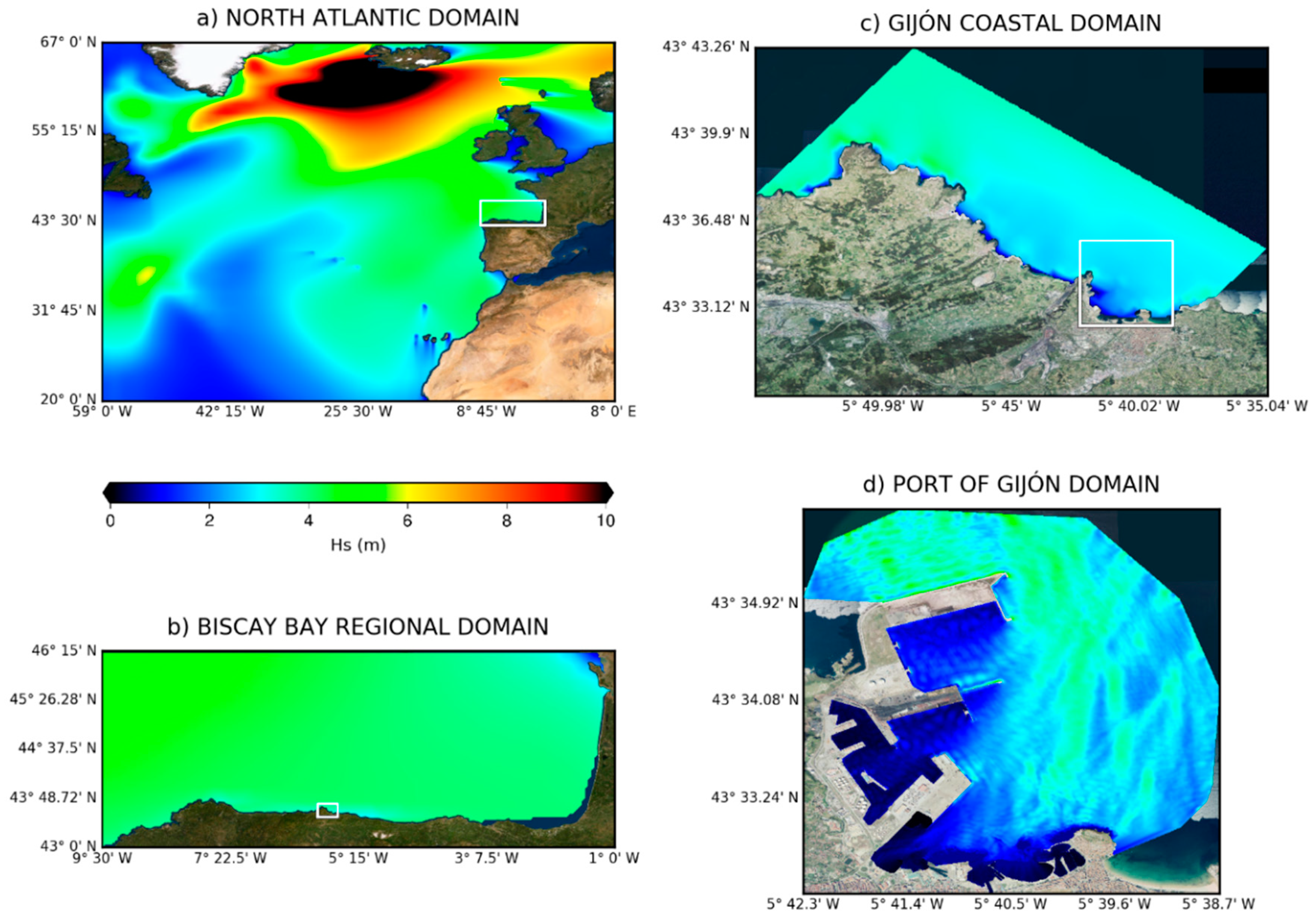
  • In Section 2, as part of the materials and methods, the downscaling approach for the climate characterization at deep waters and internal waters is described. It also contains the GCMs, concentration scenarios, and time horizons selected for assessing the impacts that changes in magnitude, frequency, duration, and direction of metocean agents can generate, as a practical application, on the Port of Gijón. This port, located in the north of Spain, was selected for being exposed to the severe wave climate of the North Atlantic domain. Strategies for the evaluation of the operability at the AOIs are also provided as well as the approaches for the identification and definition of the AOIs and operative thresholds at the Port of Gijón for the purpose of this study.
  • The results of metocean variables at deep waters and the evaluation of the operability at the Port of Gijón (Spain) are summarized in Section 3, also providing a comparative analysis of intra-model and inter-model variations.
  • Finally, a discussion of the methodology and results is presented in Section 4, together with main conclusions.

1.1. Towards the Concept of Geo-Probability: Characterization of Port Areas

Maritime and coastal engineering has addressed the knowledge and characterization of the maritime climate from the large scale and linearity to the scale of detail and highly non-linear processes.
In Spain, the first wave measurement system was installed in 1978 at deep waters (>100m) within the state REMRO program (Martinez, 2001 [7]). Since then, a network of instrumental control points has been gradually built and enhanced within the REDEXT program. This large and valuable source of information allows us to characterize and infer metocean variables in deep waters and, thanks to the REDCOS program, also in coastal environments. This data has been used, among others, to calibrate numerical models, to successfully design and build sheltering infrastructures and, ultimately, to favor port activity, which is one of the main strategic axes of the country. Monitoring inside ports started at an earlier stage (the first tide gauge of Spain was placed in Alicante in 1874), although its objective was initially to provide a reference for the elaboration of topographic maps. Later on, this instrumental information, unified inside REDMAR network (Pérez and Rodríguez, 1994 [8]), was used for a local characterization of the tidal regime. Recently, the new version of NIVMAR storm surge forecasting system (Álvarez-Fanjul et al., 2001 [9] and García-Valdecasas et al., 2019 [10]) has made it possible to further take advantage of this data for addressing in situ wave agitation or even infra-gravitational waves such as resonance events, seiches, or tsunamis. Thanks to the increase in computational capacity and the improvements in wave propagation models, the Organismo Público de Puertos del Estado (OPPE, the Spanish public organism in charge of managing state-owned ports) is offering predictions and real-time information of metocean variables at high resolution inside Spanish ports. This information is available for some pilot ports since the completion of the project SAMOA in 2017 and will be provided for most state-owned ports after finishing the second implementation of the project in 2021 (Álvarez-Fanjul et al., 2019 [11]).
Thus, we are presently on the way towards a 4.0 Port model (Molina, 2018 [12]), highly monitored not only in terms of metocean agents, but also in relation to the infrastructure and each single port operation. A model in which the physical environment is constantly measured, the infrastructure is permanently auscultated and the Key Performance Indicators (KPIs) of the operations are continuously supervised. A model in which design transcends beyond structural safety and focuses as well on the conservation, maintenance, and operability during the useful life. A model in which the whole system is deeply understood and so are their structural and operational risks. It is in this context where the concept of geo-probability is arising, as it brings together two key aspects of risk management and decision-making in ports: the probabilistic nature of the risk itself and the inherent spatiality inside port environments. The following sub-sections are aimed to expound on these two aspects.

1.2. Risk Indicators: Probability, Vulnerability, and Costs

The term “risk” has a varied number of definitions and approaches (Kaplan and Garrick, 1981 [13], Covello and Mumpower (1985) [14], Al-Bahar and Crandall, 1990 [15], Cano and Cruz, 2002 [16], NASA, 2011 [17].). As shown in Välilä (2005) [18], up to ten types of risks can be identified in projects: design, construction, service quality, demand, operational, payment, financial, political, environmental, and force majeure. Its formulation varies depending on the type of risk, but also on the economic sector. In Gómez & Molina et al. (2018) [6], a review of the concept of risk and the terms that comprise it is provided, identifying and defining two fundamental types in the port sector: infrastructural risk and operational risk:
  • Infrastructural risk is an indicator that quantifies the deviation from the objectives of reliability and functionality of the infrastructure, derived from the occurrence of failure modes.
  • Operational risk is an indicator that quantifies the deviation on the economic objectives or quality of service provision of an activity, derived from the occurrence of failure and/or stoppage modes in an area of operational interest.
Likewise, the latter reference proposes a general formulation of risk:
R = [P|V|C]
which depends on three interconnected concepts: probability (P), vulnerability (V) and consequences (C). This definition is based on the probabilistic view introduced in the Spanish Recommendation for Maritime Works ROM 0.0-01 [19] and begins with the characterization of the stochastic nature of all the elements that are part of the evaluation of the probability of failure or operational stoppage (mainly parameters and agents or threats). The vulnerability refers to how threats interact with the system and can be defined as “the degree of affection to which an element or group of elements at risk are subjected as a result of the occurrence of an event that interferes with the normal functioning of the activity for which they were designed, expressed on a scale of 0 to 1, where 0 corresponds to the non-existence of damage, and 1 to a total loss” (Molina et al., 2017 [20]). It requires, therefore, a deep knowledge of the mechanisms associated with failure/stoppage modes and the possible relationships between them, typically addressed by means of fault trees (e.g., Campos et al., 2010 [21]). A threshold approach is a simplified vision of the vulnerability: in a Boolean approach the vulnerability would be 0 when threats do not exceed a certain value and 1 when this value is overcome. Finally, addressing risk is also addressing consequences, usually quantified in terms of costs, i.e., in terms of the economic losses associated with the system response to threats. In the simplified Boolean approach, that would mean estimating the costs provoked by the exceedance of the threshold.
Risk estimation implies a high degree of particularization for each infrastructure and activity, which goes beyond the purpose of this study. In a generic and simplified way, the methodological approach proposed in Section 2 was oriented to evaluate how agitation in docks could affect the operability of port operations, excluding the economic aspect. Therefore, strictly speaking, the case study is an assessment of operational vulnerability which, applied to different climate change scenarios, allows analyzing the sensitivity of the vulnerability against different prediction horizons.

1.3. Definition of Areas of Operational Interest (AOIs)

The spatiality inside the geo-probability concept not only has to do with the local effects and how metocean agents particularly interact with the different port areas, but also with the heterogeneity of uses, typologies, means of manipulation and, ultimately, with the vulnerability of each element or system. As a reference, the importance of the spatial component is considered in the aforementioned ROM 00-0.1 [19] by means of the identification of the subsets of the structure during the design and construction phases. Extrapolating this structural approach towards an operational perspective, Molina et al. (2017) [20] and Gómez & Molina et al. (2018) [6] proposed the term AOIs to refer to “port spaces with the same functional activity, sharing infrastructural typologies, means of manipulation, land uses, etc., and which are subjected homogenously by metocean agents”.
Despite the heterogeneity of activities inside ports, Monfort et al. (2001) [22] identified six subsystems: berthing/mooring, loading/unloading, storage, handling, internal transportation and delivery/reception. The AOIs are closely related to these subsystems and can be classified into two types: terrestrial or maritime. The definition of the AOIs offers the opportunity to identify and characterize, not only each subsystem, but also the specific stoppage modes and their interconnections, as well as it permits the highlighting of which agents need to be monitored and/or modeled for being predominant in the development of these failure/stoppage modes (notice that the conceptualization of the AOIs is strongly linked to the aforementioned investment in high-resolution prediction of metocean agents inside port areas). Finally, it allows a systematic approach towards risk management, establishing a spatial structure for gathering knowledge and experience, in which the accuracy on the evaluation of each specific vulnerability and its associated costs can be gradually enhanced.
As a practical example, Section 2.4 details the process for the identification and definition of the maritime AOIs at the Port of Gijón (Spain). This subdivision of port spaces allows, for the present case study, the assessment of the vulnerability of operations at the port as well as the comparison between different GCMs, concentration scenarios, and time horizons.

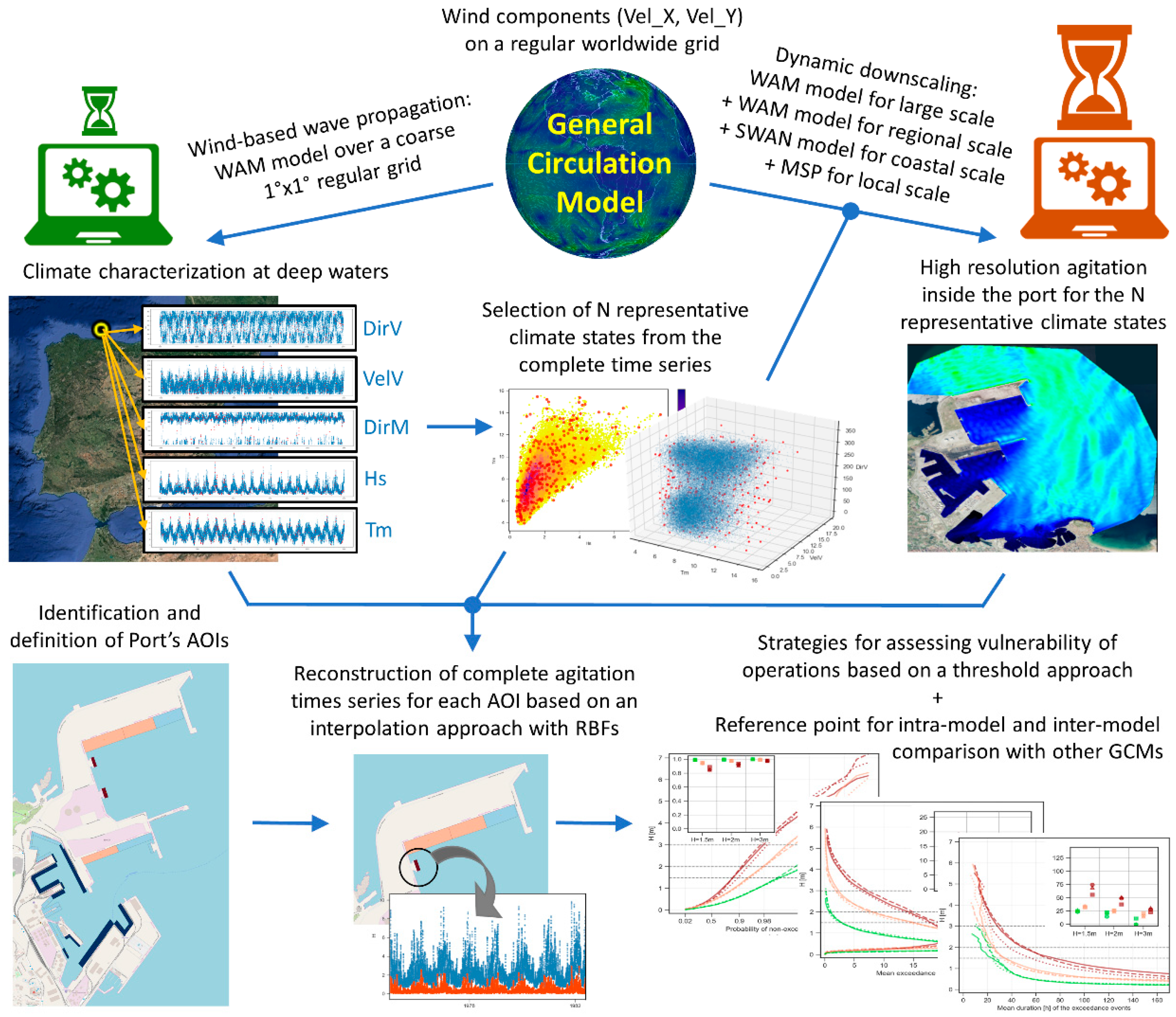
2. Materials and Methods

The first step in the evaluation of operational vulnerability in port docks under climate change scenarios is to identify potential impacts, main metocean agents involved and sources of information (Sánchez-Arcilla et al., 2016 [23]). Studies addressing the impact of climate change on ports operability are few in comparison with the ones focused on coastal areas. Some of them present strategies for assessing the vulnerability of operations with respect to overtopping (Sierra et al., 2016 [24], Camus et al., 2017 [25]). Others, such as Gracia et al. (2019) [26], relate operability with sea level rise (SLR). In addition, others, assess operability impacts considering changes in wave agitation (Sierra et al., 2015 [27]) or in the combination of wave agitation and SLR (Sierra et al., 2017 [28]). The present paper also relates downtimes with wave agitation and SLR, offering a strategy for connecting wind components from GCMs with operability indicators at each AOI of the port. These indicators are calculated using a threshold approach, based on the high-resolution wave agitation values downscaled at port areas.
The methodology applied for addressing long-term operational vulnerability in port docks under climate change scenarios is schematized in Figure 1. It can be divided into the 4 steps expounded on in the following sub-sections:
  • Climate characterization at deep waters (see Section 2.1, in which the selection of GCMs, concentration scenarios, and time horizons is also detailed).
  • Propagation to internal waters (see Section 2.2), following the hybrid downscaling method from Camus et al. (2011) [29] for reducing computational costs.
  • Evaluation of the operability at the AOIs (see Section 2.3), proposing operability indicators based on a Peaks Over Threshold (POT) approach.
  • Identification and definition of AOIs, in which the Port of Gijón, as a practical case, is divided into homogeneous areas for assessing the vulnerability of operations (see Section 2.4).

2.1. Climate Characterization at Deep Waters

To allow an inter-model/inter-scenario comparison of the results in accordance with the resources available at CLIMPACT project, three different atmospheric GCMs were selected, together with two Representative Concentration Pathways (RCPs) and three time horizons (see Table 1):
  • GCMs were selected from CMPI5 (Taylor et al., 2012 [2]), ensemble r1i1p1, an ambitious coordinated model intercomparison exercise involving most of the climate modeling groups worldwide. CMIP5 has served as an input for numerous assessments on climate change such as the IPCC Fifth Assessment Report, AR5 [1]. For this study, global wind components were downloaded from the web servers of the World Climate Research Program (WCRP) from the Working Group on Coupled Modeling (WGCM). To pick up three representative GCM, waves projections from the Commonwealth Scientific and Industrial Research Organization (CSIRO, see Hemer et al., 2015 [30]) were compared at a location close to the Port of Gijón (Spain): the point with geographical coordinates (44.5°, −5°). Based on CSIRO’s waves projections, built with atmospheric GCMs from CMIP5, a GCM with high severity of wave action was chosen, together with another one with mean severity and a third one with low severity. The selected GCMs were, respectively, the model MRI-CGCM3 (Yukimoto et al., 2012 [31]) from the Meteorological Research Institute, the model MIROC5 (Watanabe et al., 2010 [32]) from the group formed by the Atmosphere and Ocean Research Institute (The University of Tokyo), the National Institute for Environmental Studies and the Japan Agency for Marine-Earth Science and Technology and the model CNRM-CM5 (Voldoire et al., 2013 [33]) from the group formed by the Centre National de Recherches Météorologiques and the Centre Européen de Recherche et Formation Avancée en Calcul Scientifique. Other GCMs analyzed for this selection were ACCESS10, BCC-CSM11, HadGEM2-ES, and INMCM4.
  • RCP4.5 and RCP8.5 were the two concentration scenarios chosen which, as described in depth in AR5 [1], represent an intermediate climate mitigation scenario and a high greenhouse gas emissions pathway, respectively.
  • Three further 20-years spans were selected as time horizons. In line with other publications such as the aforementioned AR5 [1], the control scenario for each model was defined to be from 1986 to 2005, the short-term or mid-century scenario from 2026 to 2045, and the long-term or end-century scenario from 2081 to 2100.
For each GCM, concentration scenario and time horizon, a full global simulation with a coarse regular grid of 1 degree is computed, using wind fields as an input and obtaining a complete time series of metocean parameters near the area of study, at the deep-water location with geographical coordinates (44°, −5°). These time series, with a 3-h resolution, are then analyzed from an annual and seasonal perspective focusing both on the mean and extremal regimes.

2.2. Propagation to Internal Waters

As exposed in Section 1, mesh scale of GCMs is too coarse for considering local effects which, in the case of wave propagation, are fundamental regarding wave transformation non-linear processes derived from local interactions with the bathymetry and contours. In addition, GCMs do not simulate ocean waves and, therefore, a downscaling approach is needed to project future wave conditions. Classical methodologies for achieving high-resolution local wave climate use either mathematical tools to calculate near-shore values (also known as statistical downscaling, e.g., Casas-Prat & Sierra, 2014 [34] and Martínez-Asensio et al., 2016 [35]) or dynamic simulation of near-shore high-resolution models (e.g., Sierra et al., 2015 [27] and 2017 [28]). The latter provides better results, but at the expense of more time and resources consumption. A third methodology using a hybrid statistical-dynamic downscaling was proposed by Camus et al. (2011) [29]. Due to its efficiency and good quality of the results, the methodology applied in this study is derived from the one proposed by Camus et al.
From the time series simulated at the deep-water location, several representative climate states are selected taking into account two wind parameters (wind direction, DirV, and wind velocity, VelV) and three wave parameters (wave direction, DirM, significant wave height, Hs, and mean wave period, Tm). The multi-parametric selection of the representative cases was accomplished by applying a maximum dissimilarity algorithm: the MaxMin version described by Camus et al., 2011 [36]. This approach, proved to be quite efficient by other authors, such as Gouldby et al. (2017) [37], ensures the representation of all possible climate states in the subsequent interpolation of dynamic downscaling simulations, including extreme events. After some initial tests, 300 cases were chosen as a balance between the computational costs of the dynamic downscaling simulations and the quality of the reconstructed results at the AOIs. Notice that 300 cases represent just about 0.5% of all 3-h climate states from the 20-years spans and, thus, the computational effort of the dynamic simulations is significantly reduced.
For each of the selected metocean states, dynamic downscaling simulation is carried out with a warm-up time of 4 days. In this way, a complete propagation and simulation of sea and swell waves in the port area is achieved taking into account the past sea states capable of influencing the agitation results at the AOIs. To obtain wave interaction inside the port, a nesting methodology is required (see Table 2). The complete North Atlantic is simulated at a resolution of 25 km, nesting to a 4 km regional grid, which is then downscaled to a 300 m grid for the coastal model and to an unstructured grid resolving the port area. Figure 2 shows a schematic view of the dynamic downscaling approach that has been applied in this study. The Spanish national models from the OPPE were computed for the simulations: WAM models (WADMI Group, 1988 [38], Guenther et al., 1992 [39]) for large and regional scales, a SWAN model (Booij et al., 1996 [40]) for the coastal area and a MSP model (Berkhoff, 1976 [41], Porter, 2003 [42]) for the local area.
As sea level influences the propagation of waves near-shore, it needs to be taken into account. As with Sierra et al. (2017) [28], a mean level is assumed for the calculation of operational descriptors and SLR was considered to be the mean value along each time horizon. SLR time series were analyzed from the regional sea level data considered in AR5 (distributed by the Integrated Climate Data Center of the University of Hamburg, Hamburg, Germany) at the point with geographical coordinates (44.5°, −5.5°). The control scenario was assumed to be associated with a zero value of SLR, whereas the short-term and long-term scenarios were propagated respectively considering a SLR of 0.155 m and 0.438 for the scenario RCP4.5 and a SLR of 0.164 m and 0.587 m for the scenario RCP8.5.
Once the dynamic downscaling simulations are completed, several agitation values from the high-resolution local domain are enclosed within each AOI. The percentile 98 is then calculated as a stable indicator of the upper tail and, thus, of the most unfavorable agitation conditions (rather than using the maximum value, typically subjected to a lesser numerical certainty, especially a model’s contours). Finally, the complete agitation time series at each AOI is reconstructed by means of an interpolation approach with Radial Basis Functions, RBFs (Camus et al., 2011 [29]), relating all the multidimensional metocean states (DirV, VelV, DirM, Hs, Tm) at the deep-water location with the mono-parametric agitation outputs (H) calculated for each of the selected cases.

2.3. Evaluation of the Operability at the AOIs

Operability is defined in the Spanish Recommendation for Maritime Works ROM 0.0-01 [19] as the “complementary value of the overall probability of stoppage in the project phase against the principal stoppage modes, ascribed to all of the stoppage limit states”. Therefore, the first step to its evaluation is to characterize all stoppage modes and combinations between them for each operation carried out at each AOI. For a cargo loading/unloading operation, this would depend on the cargo type, handling means, vessel type, vessel size, load level, movements induced by metocean agents and expertise of human factors, among others. It is, therefore, a multidimensional problem with many degrees of freedom and a high level of particularization (ROM 2.0-11 [43], PIANC [44,45] and Molina, 2014 [46]). The monitoring trend towards a 4.0 Port model exposed in Section 1.1 will presumably shed further light on this challenge that, so far, has been faced combining a mono-parametric perspective regarding metocean agents (mainly wind velocity and wave agitation) and a threshold approach. Notice that defining, for example, a wave agitation threshold of 1 m for forecasting whether a cargo loading/unloading operation will be carried out or not is quite a simplistic approach and, at the same time, it requires expert criteria and deep knowledge about that operation in particular. Indeed, most studies found in the literature applying a threshold approach to maritime operations are focused on singular maneuvers (Cabrerizo-Morales et al., 2012 [47] and Cabrerizo-Morales et al., 2018 [48]).
Being the accurate characterization of the operability out of the scope of this work, a slight enhancement complementing the traditional threshold approach is proposed. Usually, the probability of a stoppage of a maritime operation is linked to the probability of exceedance of a certain agitation value. However, in a real case (assuming that exceeding that threshold always triggers the stoppage), there is another variable to take into account: the maximum duration between exceedance events for being considered inside the same downtime case. In other words, an operation will not be resumed if the threshold is forecasted to be exceeded again soon. Therefore, lower agitation values than the threshold can be part of a stoppage and, thus, a POT analysis might be more adequate. POT analysis offers the possibility of counting the number of events and the duration of each of them. It also allows consideration of two exceedance events inside the same episode if the span between them does not overcome a certain limit duration.
If a POT is applied to each of the unique values of an agitation time series, graphs such as the ones in Figure 3 are obtained. This approach presents the advantage of providing operational information for every agitation value and, thus, it is flexible for any threshold defined. Furthermore, this approach can also be helpful as a port management decision-making tool, especially when assessing metocean variations due to climate change: if applied to every AOI inside a port, it offers a complete vulnerability map opening up doors to promote adaptation strategies (such as re-allocating activities according to the desired operability) or mitigation strategies (such as investing in new sheltering infrastructures) when the economic activities are not compatible with the conditions to come.

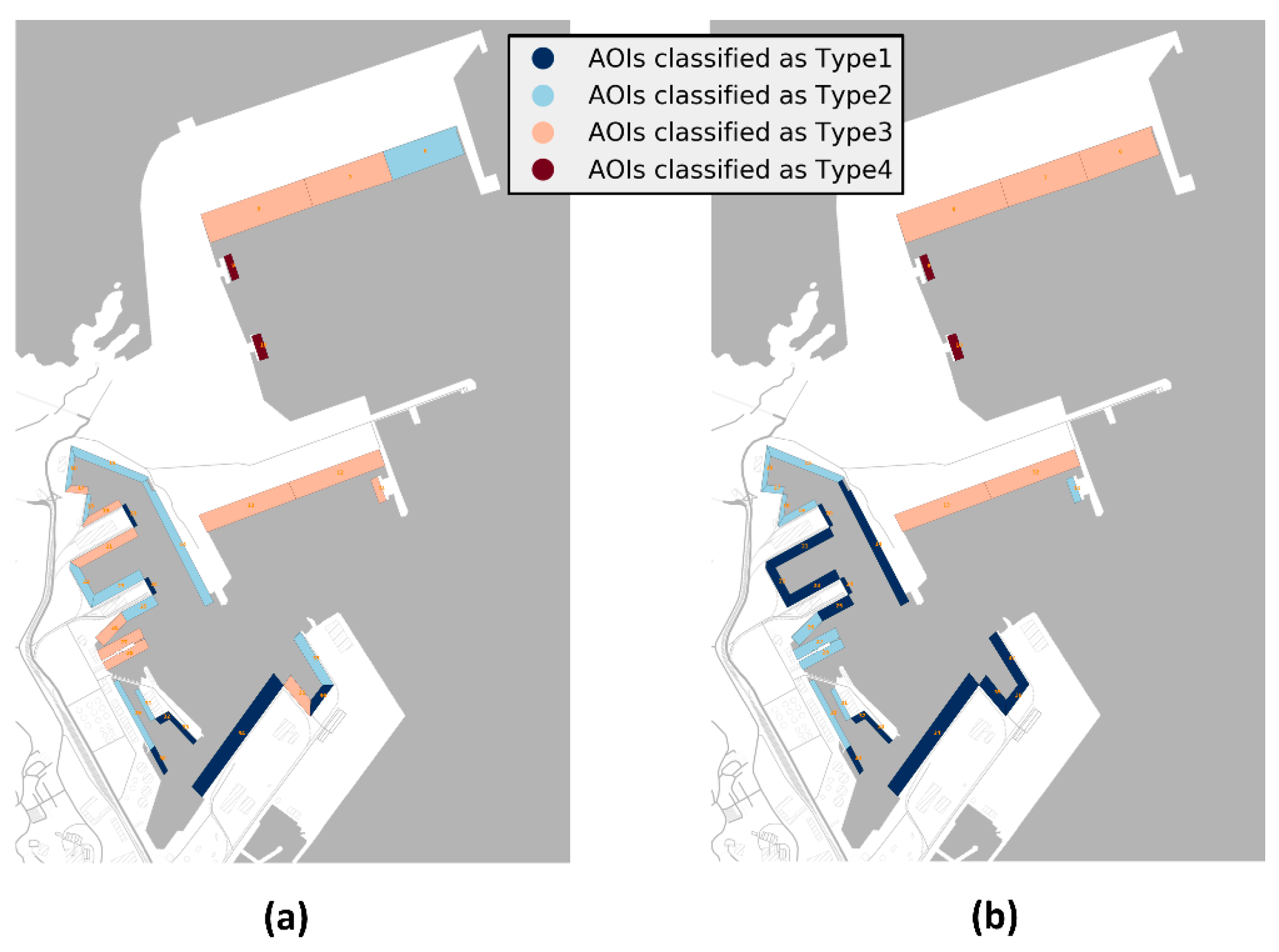
2.4. Identification and Definition of AOIs: Application to the Case Study

As has been exposed in Section 1, one of the contributions of this study is to propose an approach towards the concept of geo-probability in ports management based on previously identifying the AOIs of the port. Dealing presently with the opportunity of increasing the accuracy and spatial resolution of metocean predictions, this approach allows spatial analysis of the interaction of metocean conditions with the particular operations and activities carried out inside ports.
For the sake of simplicity, terrestrial AOIs are dismissed in this study and, thus, the spatial characterization of the Port of Gijón is focused on main maritime areas. These areas are linked to economic activities in which operations such as mooring/unmooring of vessels, embarking/disembarking of passengers or loading/unloading of goods are carried out. A total of 32 AOIs were proposed after a cross analysis of infrastructures, handling means, economical activities, type of vessels, bathymetry, and exposure conditions to metocean agents. Therefore, the relatively complex and heterogeneous structure of the whole port is split into homogeneous areas in which operational vulnerability analysis can be individually addressed. The length of each AOI is related to all the aforementioned factors, whereas the width of each AOI was defined to be 2.5 times the mean beam of the ships that are identified to be operating in the area. Combining both sizes, the proposed AOIs go from 2000 m2 for the smaller ones up to 80,000 m2 for the biggest one located at the northern enlargement.
Not only is the approach towards the concept of geo-probability in ports management one of the aims of this study, but it is also to provide a methodology to implement the latter together with strategies for addressing long-term operational vulnerabilities under different climate change scenarios. Taking into account that 3 different models were propagated, together with 2 concentration scenarios and 3 time horizons (see Section 2.1), adding further 32 AOIs to the present case study was likely to jeopardize the visualization and interpretation of annual and seasonal operational results due to the high amount of information. Therefore, it was decided to simplify this example by classifying AOIs into four types to be able to focus the analysis on four mean operability trends. Two possible classification strategies were identified (see Figure 4):
(a)
Attending to the operational vulnerability of their current real activities to wave agitation by taking into account the thresholds proposed in the Spanish Recommendations for Maritime Works ROM 3.1-99 [49]. The most vulnerable activities were classified as “Type1” and included any of the following vessel typologies: liners, cruises, ferries, Ro-Ros, container ships, or fresh-fish fishing boats. “Type2” grouped all AOIs with general cargo merchant ships or deep-sea fishing boats. “Type3” involved bulk carriers, liquid gas carriers, or small oil tankers. Finally, AOIs with least vulnerable activities against wave agitation, carried out by larger oil tankers, were grouped into “Type4”. This approach, despite being realistic, was rejected for not being homogeneous from the point of view of the operability. For example, assuming that loading/unloading stoppage is caused by overcoming a certain wave agitation threshold, the fact of allocating activities classified as “Type3” in highly sheltered basins allows avoiding downtimes. However, at the same time, the most exposed basins are just compatible with “Type3” or “Type4” activities, being likely to undergo operative stoppages despite their lesser vulnerability in comparison with “Type 1” or “Type 2”. Consequently, the mean value of the number of stoppages for all “Type3” AOIs would not be representative of the trend at the most exposed AOIs nor at the most sheltered ones.
(b)
Attending to a homogenous wave agitation criterion by considering all the propagated metocean scenarios described in Section 2.1, to avoid the latter constraint. For each scenario, different percentiles (50, 98 and 100) of the propagated wave agitation inside the contours of each AOI were calculated and, based on that, AOIs were classified into four groups. After evaluating all scenarios, each AOI was assigned the class with more matches, being “Type1” the least exposed and “Type4” the most exposed. In this way, when calculating operability trends for each typology, mean values are indeed representative of the particular trends of each AOI in the group, as shown in Figure 5.
Three different thresholds were assigned to each AOI (see Table 3). Despite been based on the limit operating conditions at quays and jetties from ROM 3.1-99 [49], these thresholds are not intended to be representative of real operations at every single AOI. They are established for the sole purpose of providing references for an inter-model and intra-model comparison between the propagated results from the scenarios selected in Section 2.1.

3. Results and Discussion

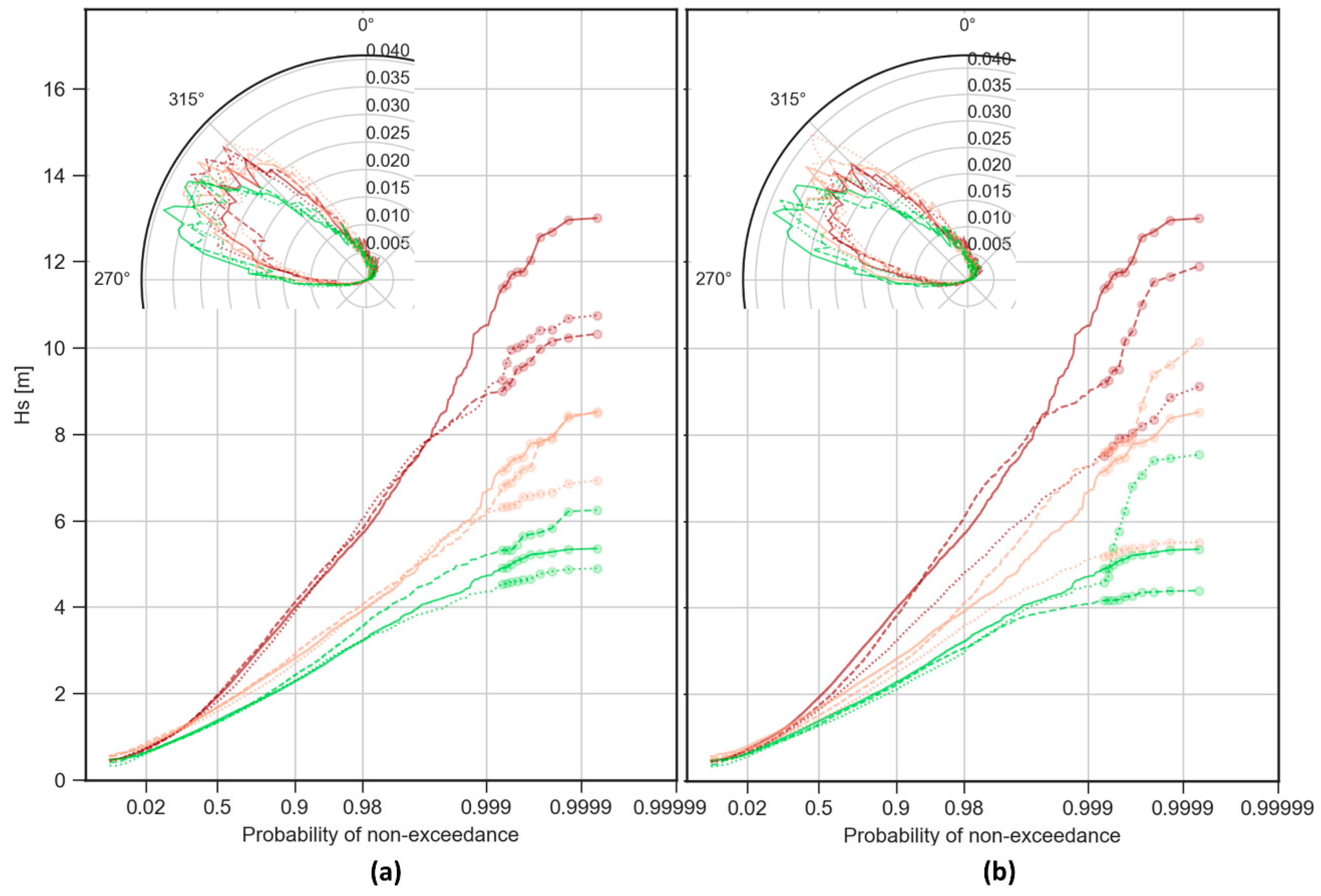
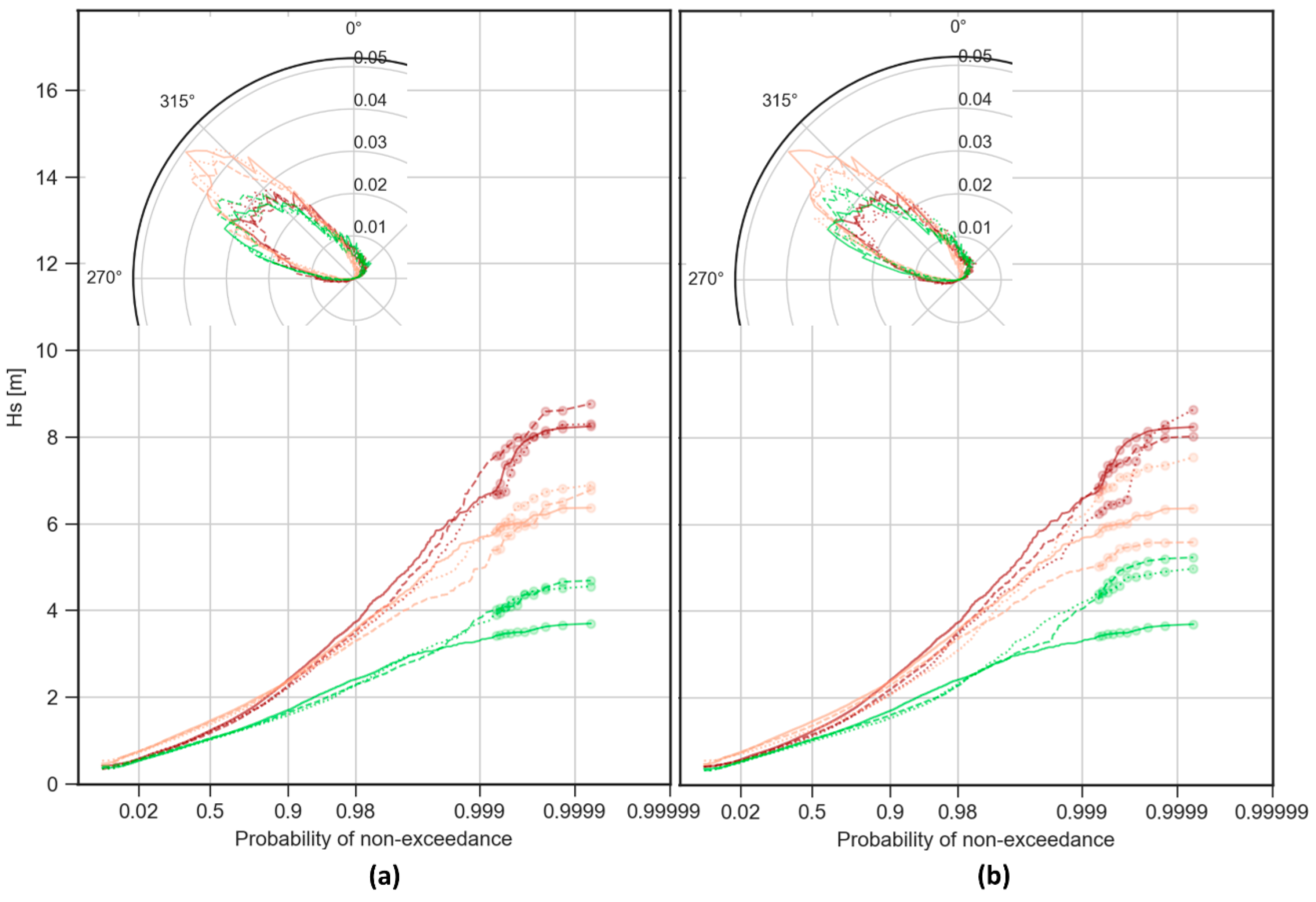
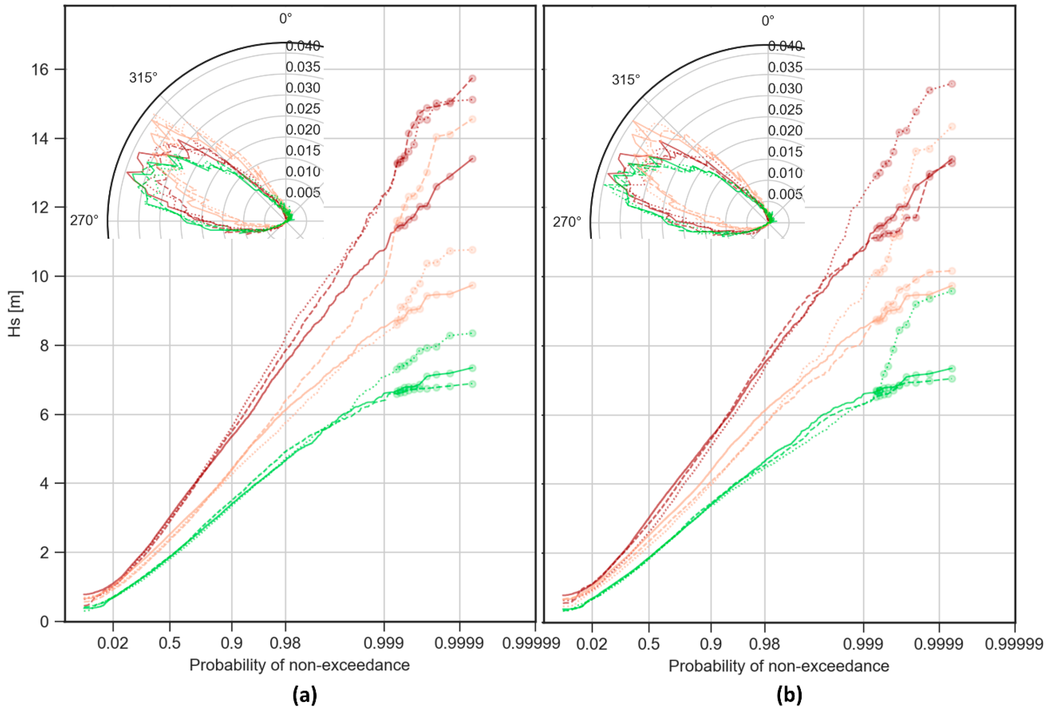
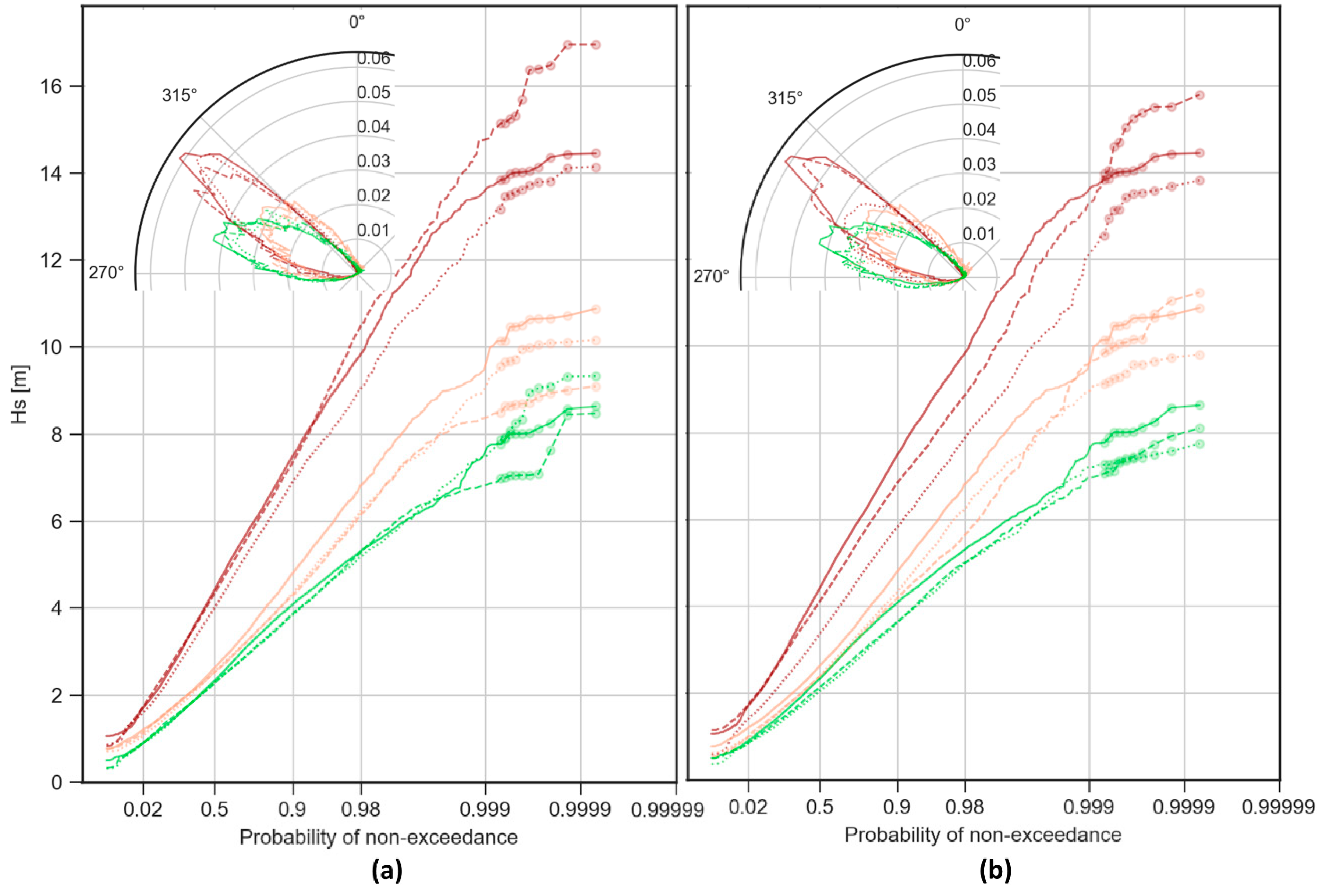
3.1. Inter-Model and Intra-Model Comparison of Significant Wave Height (HS) at the Deep-Water Control Point Outside the Port of Gijón (Spain)

Before addressing the operative descriptors inside port AOIs (see Section 3.2), an initial analysis of the propagated values of the significant wave height (HS) at the deep-water control point with coordinates (44°, −5°) for the different GCMs, concentration scenarios, and time horizons is accomplished. Table 4 presents annual and seasonal statistics for the control scenarios of each GCM, whereas Table 5 summarizes the variations of all the other propagated scenarios in comparison with the control ones:
The first conclusion, which is in line with other publications (Sierra et al., 2015 [27]), is the large inter-model variability, more noticeable than the intra-model variability regarding the different concentration scenarios and time horizons. This variability is especially evident for the highest values of HS, with differences between control scenarios up to 3 m for the maxima. In general, mean values and all other descriptors except maxima tend to decrease in future scenarios, being more remarkable at long-term and RCP8.5 scenarios, with a maximum reduction of 16% for the most severe GCM. These results agree with other regional studies applied in the North Atlantic sub-basin, such as the ones based on statistical downscaling and weather types from Pérez et al., 2015 [50]. Their conclusion about this finding was that “this decrease is due to a higher occurrence of dominant and moderate Azores high pressure systems over the North Atlantic Ocean and a decrease in the persistence of intense low-pressure systems at high latitudes”. This trend is also present from a seasonal point of view, in which the highest reductions seem to be concentrated in winter with a maximum decrease of 22% for the most severe GCM. When analyzing maximum values, trends are more unstable, as so is the reliability of this statistical descriptor, likely to be able to substantially differ between different realizations of the same forcing scenario. Maxima tend to increase for most future scenarios, with up to 34% for the most severe GCM. From a seasonal point of view, the two most severe GCMs tend to increase maxima in autumn, with up to 49% increase for the medium model, and tend to decrease maxima in spring, especially for the RCP8.5 scenario. The least severe GCM shows more erratic trends of the maxima, with the solely identification of a clear increase during summer.
The analysis of the statistics is complemented with Cumulative Distribution Functions (CDFs) of HS and details of the polar Probability Density Functions (PDFs) of wave directions for short-term scenarios and for long-term scenarios. In Figure 6 the complete datasets are presented, whereas a seasonal analysis is provided in Appendix A (see Figure A1, Figure A2, Figure A3 and Figure A4). CDFs are represented in Gumbel probability paper for maxima and, to provide information about the dispersion of the upper tail, the 10 most extreme values are highlighted with dots. Polar PDFs of wave directions are aimed to illustrate inter-model and intra-model differences, as changes in wave direction are also likely to modify wave agitation inside ports. In line with the aforementioned conclusion after addressing the variations of HS, wave direction also shows a dominant inter-model variability. Seasonally speaking, most wave directions are concentrated between W and NW in autumn and, especially, in winter. In spring, and more manifest in summer, the probability of directions between NW and NE are also of relevance. No clear trend in the variation of wave direction due to the different concentration scenarios or time horizons was identified.

3.2. Characterization of Wave Agitation in the AOIs of the Port of Gijón (Spain). Inter-Model and Intra-Model Comparison of Operational Descriptors Based on a Mono-Parametric Thresholding Approach

Following the methodology described in Section 2.2, wave agitation (H) is calculated for each of the GCMs and scenarios specified in Section 2.1. Three different analysis were accomplished for the unique values of H at each AOI: probability of non-exceedance (PROB), mean number of exceedance events per year (N) and mean duration of the exceedance events (T). The individual trends of PROB, N and T for each AOI were grouped afterwards in a mean trend for each of the four typologies defined in Section 2.4 and compared annually and seasonally among the different GCMs, concentration scenarios, and time horizons.
Exceedance events are calculated through a POT technique (see Section 2.3), assuming a minimum of 48 h for independence between events. POT is a commonly used technique when addressing operability, as stoppages might not only be linked to overcoming a certain wave threshold, but they are also likely to include the span between non-independent overcoming events. Following this approach, N represents the mean number of stoppages per year when considering as an operative threshold each unique value of the time series of H. Similarly, T represents the mean duration of the stoppages when considering as an operative threshold each unique value of the time series of H. Graphical results from a short-term and long-term analysis of the three operability indicators (PROB, N and T) are provided in Appendix A for the four different AOIs typologies defined in Section 2.4 (see Figure A5, Figure A6, Figure A7 and Figure A8).

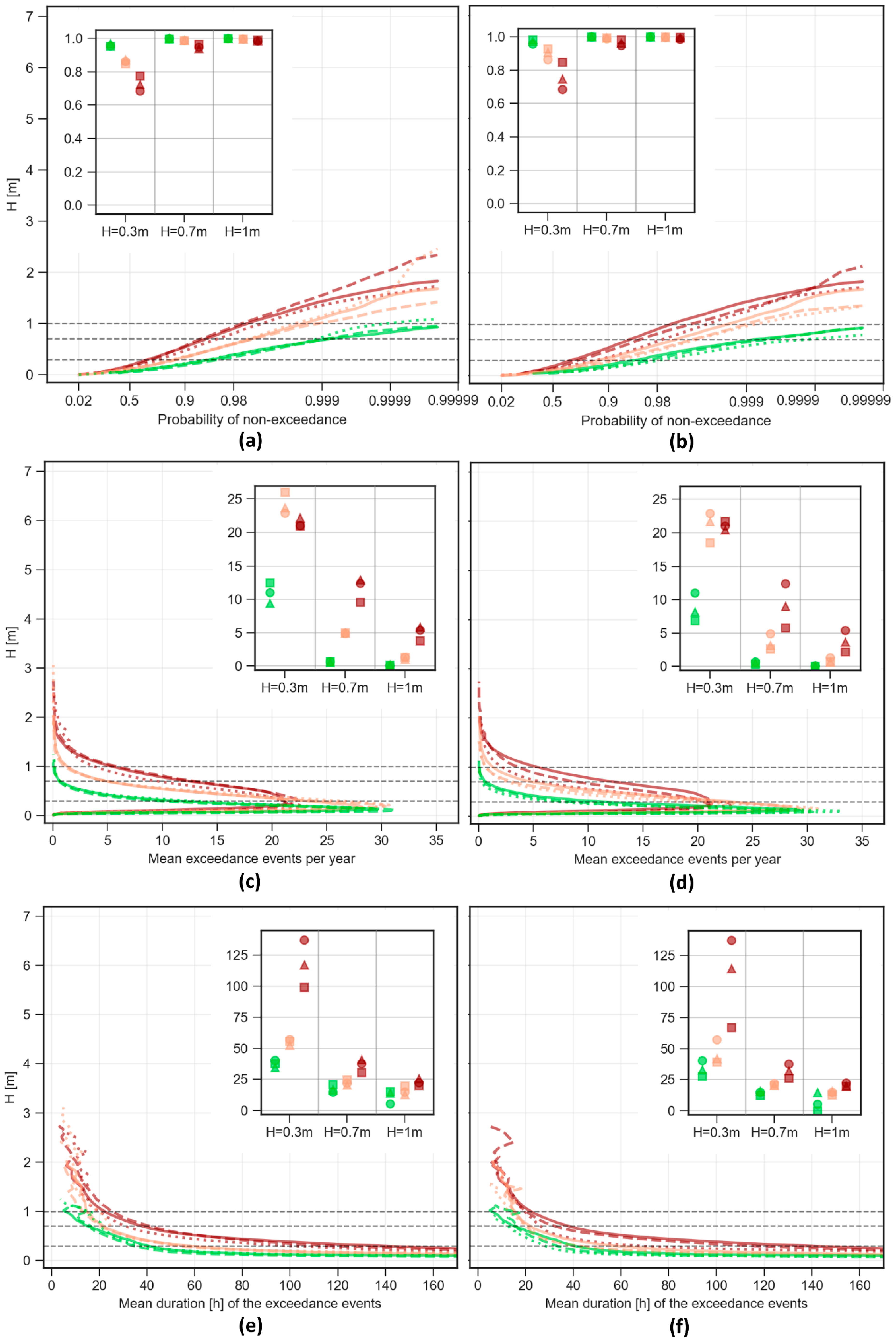
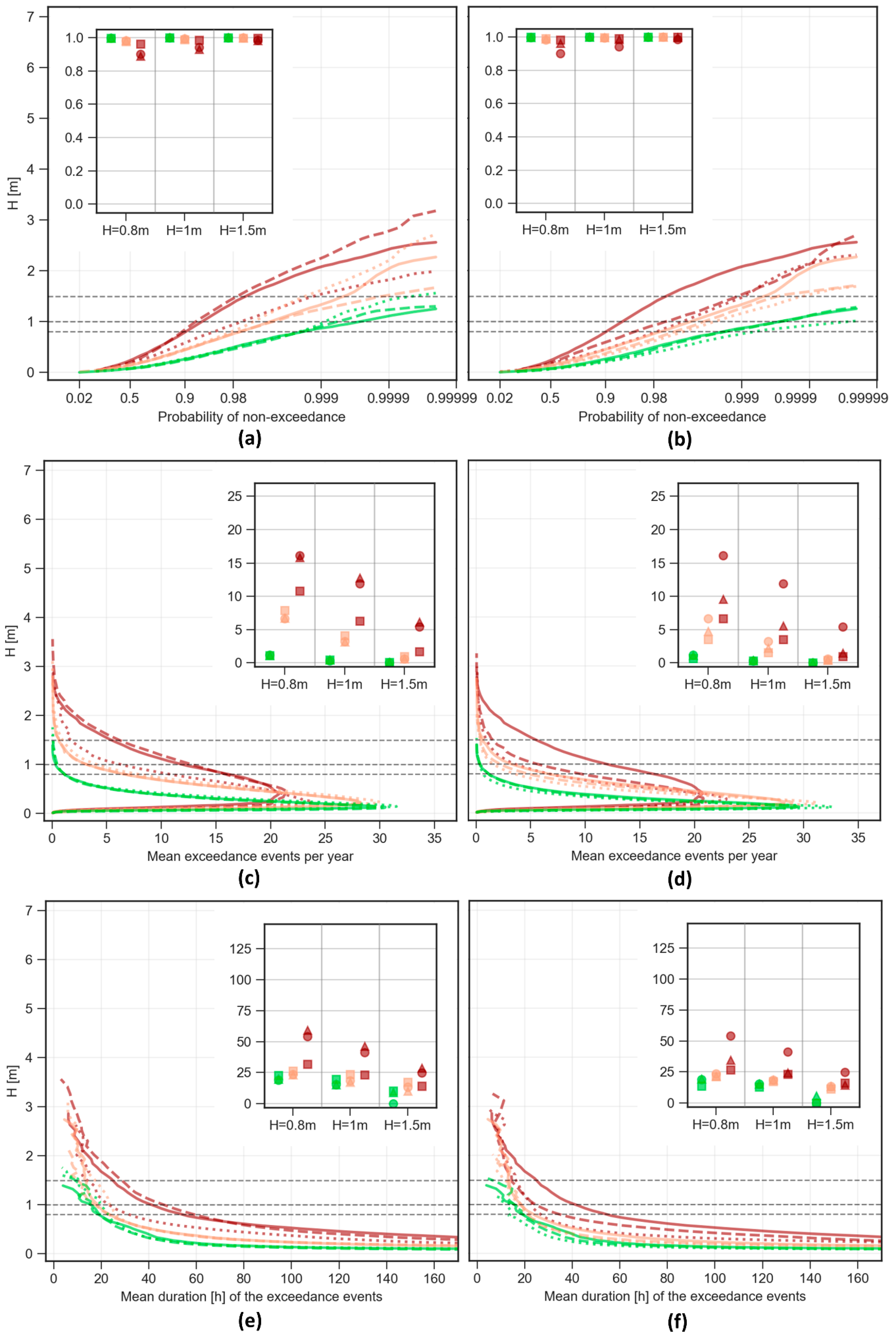
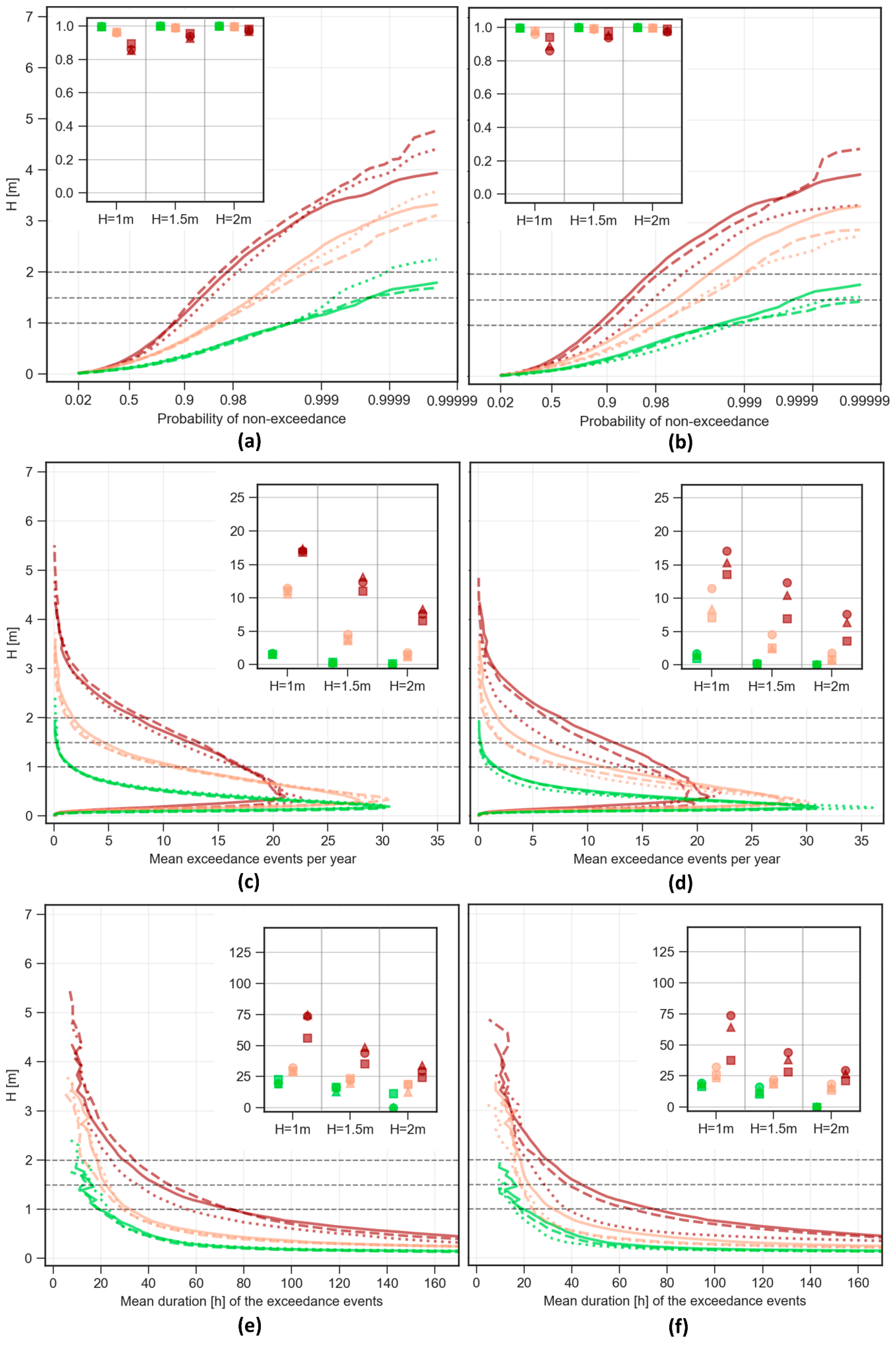
3.2.1. Operability Indicator 1: Probability of Non-Exceedance, PROB

Regarding PROB results, the first conclusion is in line with the one derived from the results at the deep-water control point: there is a large inter-model variability, especially evident for the highest values of H. As expected, the interaction with sheltering structures and bathymetry leads to differences between deep-water scenarios and the ones at the AOIs. Yet, as a similarity, values not belonging to the upper tail tend to decrease in future scenarios, which is more remarkable at long-term and RCP8.5 scenarios. Again, maxima and upper tail trends present noticeable inter-model and intra-model differences. For long-term RCP8.5, the upper tail is below the control scenario for all GCMs and typologies. Notice that, due to the high inter-model variability, thresholds assigned to each AOI group (see Table 3) perform differently for each GCM. For example, whereas the highest threshold is associated with an operability of about 98% for all scenarios of the most severe GCM, in most cases the mildest GCM is unlikely to reach that value. (Notice that the probability of non-exceedance is likely to underestimate the concept of operability, as it is not considering spans between non-independent overcoming events.)

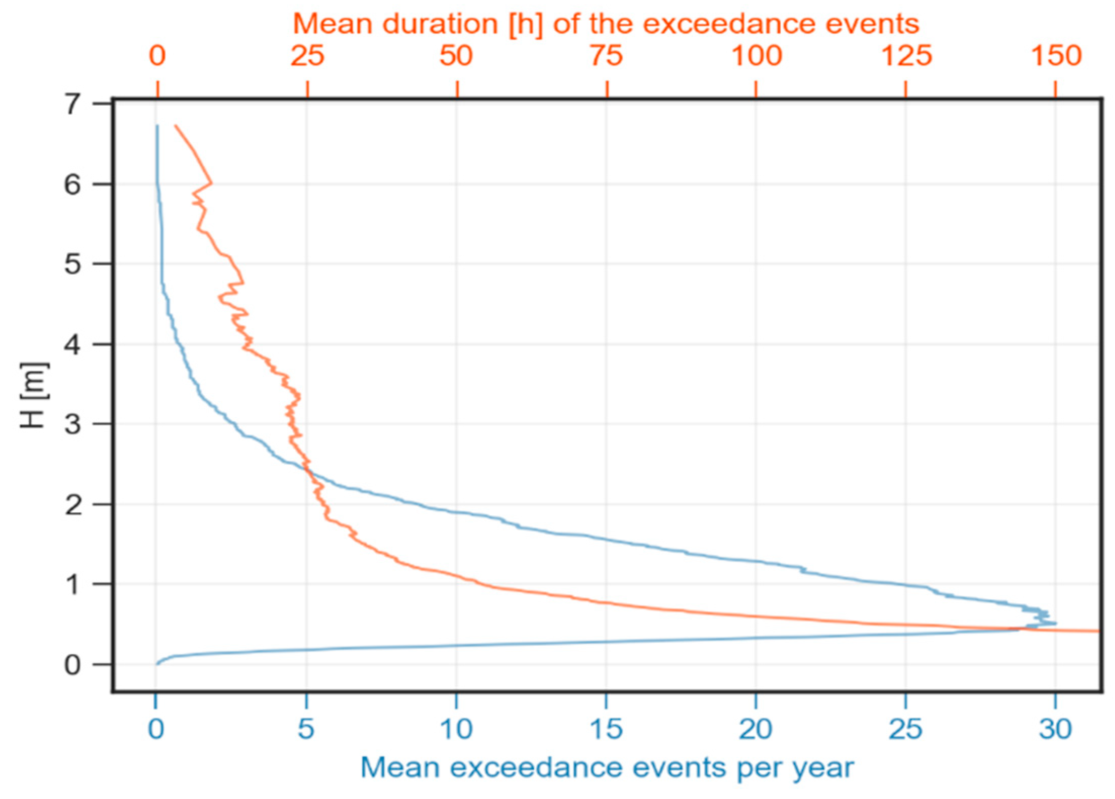
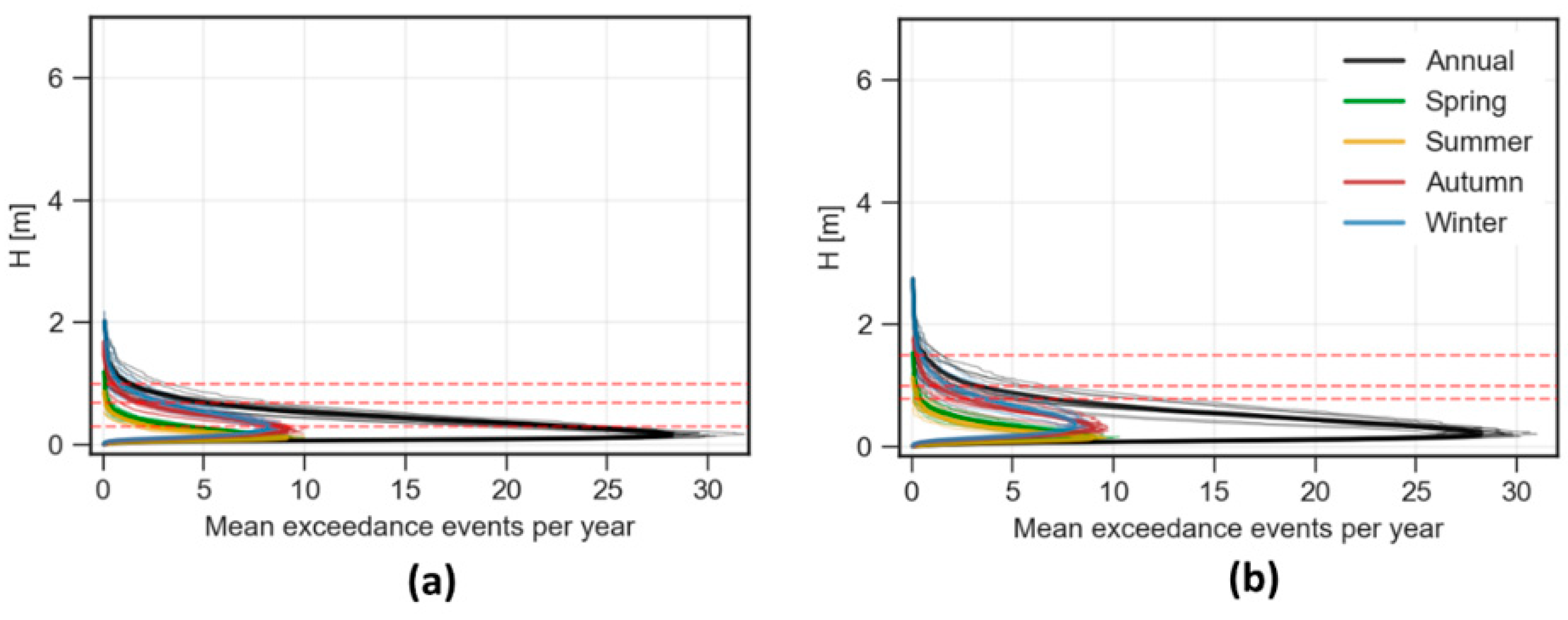
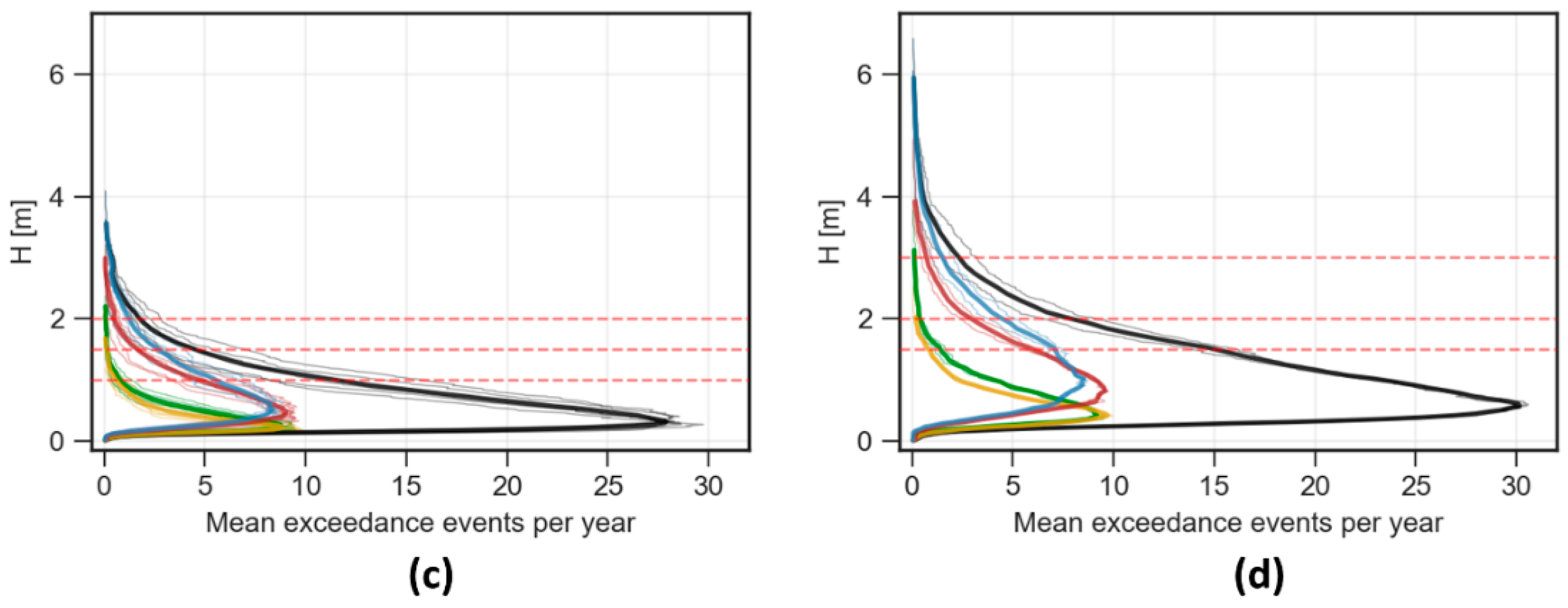
3.2.2. Operability Indicator 2: Mean Number of Exceedance Events per Year, N

Moving forward to N results, it is identified, as expected, that the number of mean stoppages per year is inversely proportional to the agitation threshold. However, there is always an inflection point at the bottom tail since lower agitation values are permanently or frequently exceeded (i.e., N is equal to 1/20 for the minimum agitation value as it represents one permanently exceeded event during the 20-year span). The inter-model variability is also noticeable for N results. Focusing on a threshold analysis:
  • Long-term scenarios show a similar pattern for most GCMs and typologies: control scenarios are related to the highest values of N, RCP8.5 scenarios with the lowest and RCP4.5 scenarios between the two of them. The mildest GCM barely overcomes, in most cases, the established thresholds for each AOI group. For the control scenario of the most energetic one, N goes from 16 to 21 for Threshold1 (for all AOI groups), from 12 to 14 for Threshold 2 and from 5 to 8 for Threshold3. The results of the aforementioned control scenario are reduced for the most energetic GCM at a mean rate of 24% in RCP4.5 scenario and a mean rate of 46% in RCP8.5 scenario. For the control scenario of the intermediate GCM, N is mostly between a half and a quarter of the ones from the most energetic GCM. A reduction of 35% for RCP4.5 scenario and 44% for RCP8.5 scenario is found for this intermediate GCM with respect to its own control scenario.
  • Short-term scenarios show a higher variability between the intra-model trends for each GCM. Again, the mildest GCM has the lowest exceedance events, close to 0 for the second and third thresholds and up to a maximum of 12 events for the first threshold at Type1 AOIs. In line with long-term results, RCP8.5 values are also reduced in comparison with the control scenario for the most energetic GCM, in this case at a mean rate of 20%. On the contrary, RCP4.5 values are usually higher than the control scenario, with a mean rate of 6%. For the intermediate GCM, two behaviors are identified. For Types 1 and 2, RCP4.5 is very similar to the control scenario whereas RCP8.5 tends to be 10% higher as an average. However, for Types 3 and 4 both scenarios tend to have fewer stoppages in comparison with the control scenario, with a mean rate of 6% for RCP4.5 and 7% for RCP8.5.

3.2.3. Operability Indicator 3: Mean Duration of the Exceedance Events, T

Finally, regarding T results, it is shown that mean duration of exceedance events is inversely proportional to the agitation threshold, although there are some peaks at the upper tail, where the differences between each independent event are able to condition the calculation of the mean value. Once again, the inter-model differences are larger than the intra-model differences. Focusing on the threshold analysis, the results from the control scenario of the most severe GCM are about two times the ones from the intermediate one and about three times the one from the mildest. As a reference, the control scenario from the most severe GCM is associated with durations between 54 h and 137 h for Thresholds1 (for all AOI groups), between 38 h and 49 h for Thresholds2 and between 22 h and 30 h for Thresholds3.
  • For long-term scenarios, control results are reduced in all models for RCP8.5 scenario at a mean rate of 37% for the most energetic GCM, 16% for the intermediate GCM and 12% for the mildest GCM. For RCP4.5 scenario, control results are reduced at a mean rate of 21% for the most energetic GCM, 10% for the intermediate GCM but are increased at a mean rate of 12% for the mildest GCM.
  • Again, for short-term scenarios there is a higher variability between the intra-model trends for each GCM. For RCP8.5 scenario, control values are always reduced at a mean rate of 27% for the most energetic model but tend to increase at a mean rate of 12% and 17% for the intermediate and the mildest GCM, respectively. For RCP4.5 scenario, control values tend to be reduced at a mean rate of 10% for the intermediate GCM but tend to increase at a mean rate of 7% and 17% for the most and the least energetic GCM, respectively.

4. Conclusions

The present paper summarizes the works from the Spanish sub-project CGL2014-54246-C2-2-R (CLIMPACT2). This sub-project was developed for assessing operational risk management at port scale in the present and future scenarios. A general methodology was proposed and applied to a pilot case at Gijón (Spain) to address an initial sensitivity of the results. The hybrid downscaling methodology, based on Camus et al. (2011) [29], has proven to be highly efficient to reduce the computational costs of the numerical propagations fed with wind velocities and directions from GCMs. In line with Sierra et al. (2017) [28], sea level was introduced as a mean value on each simulated span regarding SLR and as a mean level regarding astronomical tide. This approach can be enhanced by considering a variable SLR on each propagated sea state related to the different prediction models. As a shortcoming of this methodology, variations of sea level due to storm surge or set-ups cannot be considered in the propagation model so far. Finally, the concept of geo-probability was introduced in the study of port operability by means of the spatial characterization of AOIs. Notice that, despite this study is not considering changes in the bathymetry or geometry of the harbor, nor variations in vessel operational capabilities, these changes (indeed likely to occur) can be easily updated in the methodology by revising the contours of the numerical model and modifying the operative thresholds respectively.
Three GCMs were selected for applying the methodology to the case study: one with severe wave action at the pilot location (MRI-CGCM3), an intermediate one (MIROC5) and a mildest one (CNRM-CM5). Two concentration scenarios were added (RCP4.5 and RCP8.5), as well as three time horizons: a control scenario (1986–2005), a short-term scenario (2026–2045) and a long-term scenario (2081–2100). Wave agitation was calculated at 32 AOIs inside the Port of Gijón (Spain) and their results were analyzed and grouped in four typologies. The results show, in line with other publications such as Sierra et al. (2015) [27], that inter-model differences are more significant than intra-model differences derived from the evaluation of dissimilar time horizons or concentration scenarios. This highlight, beyond the results themselves, the importance of a concise and systematic methodology for being able to compare operational risk management results. It also emphasizes the need for a modular/flexible approach, such as the one presented herein, to be able to automatically update the process together with future GCMs.
Wave height results at the deep-water control point close to Gijón (Spain) reveal that, in general, mean values of significant height and other statistical descriptors (such as H1/3, H1/10 or H98), tend to decrease in future scenarios. This decrease is more remarkable at long-term and RCP8.5 scenarios. This is in line with other regional studies applied in the North Atlantic sub-basin, such as the ones based on statistical downscaling and weather types from Pérez et al. (2015) [50]. Maxima trends are more erratic but tend to increase according to the evaluated future scenarios; however, maxima are usually not of interest from the point of view of the operability. Assuming the generally extended hypothesis that operability inside a port depends on overcoming a certain wave agitation threshold, the aforementioned wave height reduction outside the port could be expected to increase operability inside the port. However, wave period and wave direction also play an important role in the downscaling process and in how wave action may affect operations at quays and jetties (i.e., changes in wave direction can lead to a higher wave penetration at unsheltered directions). Indeed, in short-term scenarios, increases in the mean number of operative stoppages per year were identified, as well as increases in the mean duration of these stoppages in comparison with control scenarios. In long-term scenarios most results seem to be associated with a reduction of operative stoppages and, thus, with an increase in operability, although the reliability of these predictions is lesser in comparison with short-term ones.
Regarding the aforesaid inter-model variability, the challenges and uncertainties faced presently by GCMs suggest being cautious in the interpretation of operational results inside harbors, at least for the present case study. Nevertheless, it is expected that the methodology proposed herein, connecting global models with an approach to address the vulnerability of operations at port scale, would help to update and include new criteria for the evaluation of failure modes and stoppage modes under future scenarios in a systematic and agile way.

Author Contributions

Á.C.: Data curation, Formal analysis, Investigation, Methodology, Project administration, Resources, Software, Validation, Visualization, Writing—original draft, Writing—review and editing; J.M.G.-V.: Data curation, Investigation, Methodology, Software, Validation, Writing—original draft, Writing—review and editing; R.M.: Conceptualization, Funding acquisition, Methodology, Supervision, Writing—original draft, Writing—review and editing; C.C.: Conceptualization, Funding acquisition, Methodology, Supervision, Writing—original draft, Writing—review and editing; E.Á.-F.: Conceptualization, Funding acquisition, Methodology, Supervision, Writing—review and editing; J.S.: Writing—review and editing.

Funding

This research was partially funded by the Spanish Ministry of Economy and Competitiveness, grant number CGL2014-54246-C2-2-R, under CLIMPACT Project, Sub-project 2: Economical and environmental impacts on coast and ports due to climate change: sensitivity of risk management in ports due to climate change.

Acknowledgments

Authors are indebted in first place to the Spanish Ministry of Economy and Competitiveness for funding CLIMPACT Project Sub-project 2. They are also indebted to the University of Hamburg (Germany) for the Regional sea level data from IPCC AR5 distributed in netCDF format by the ICDC (icdc.cen.uni-hamburg.de), to the CSIRO for the waves projections next to Gijón (Spain) and, last but not least, to the WGCM for the GCMs distributed in netCDF format as part of the CMIP5 of the WCRP.

Conflicts of Interest

The authors declare no conflict of interest. The funders had no role in the design of the study; in the collection, analyses, or interpretation of data; in the writing of the manuscript, or in the decision to publish the results.

Acronyms

AOIArea of Operational Interest
AR5Fifth Assessment Report from the IPCC
CDFCumulative Distribution Function
CMIP5Phase 5 of the Coupled Model Intercomparison Project
CNRM-CM5CMIP5 Coupled Model from the Centre National de Recherches Météorologiques
CSIROCommonwealth Scientific and Industrial Research Organization
DirMWave direction
DirVWind direction
DWTDead Weight Tonnage
ESMEarth System Model
GCMGeneral Circulation Model (also referred as Global Climate Model)
hHour
HWave agitation (inside port areas)
HSSignificant wave height (average height of the highest third of all waves)
HS, 1/XAverage height of the highest 1/X of all values of HS
HS, XPercentile X of all values of HS
HS, maxMaximum all values of HS
ICDCIntegrated Climate Data Center
IPCCIntergovernmental Panel on Climate Change
KmKilometers
KPIKey Performance Indicator
mmeters
MIROC5CMIP5 Model for Interdisciplinary Research on Climate
MRI-CGCM3CMIP5 Coupled General Circulation Model from the Meteorological Research Institute
MSPMild Slope Program (wave model)
NMean exceedance events per year (after applying a POT analysis)
NetCDFNetwork Common Data Form
NIVMARSistema de previsión a corto plazo del NIVel del MAR del OPPE (Spanish storm surge forecasting system)
OPPEOrganismo Público de Puertos del Estado (Spanish public organism in charge of managing state-owned ports)
PDFProbability Density Function
PIANCPermanent International Association of Navigation Congresses
POTPeaks Over Threshold
PROBProbability of non-exceedance
RBFRadial Basis Functions
REDCOSRED COStera de boyas de oleaje del OPPE (Spanish Coastal buoy network)
REDEXTRED EXTerior del OPPE (Spanish deep-water buoy network)
REDMARRED de MAReógrafos del OPPE (Spanish harbor tide gauge network)
REMRORed Española de Medida y Registro de Oleaje (Spanish network for measuring and recording waves)
RCPRepresentative Concentration Pathway
ROMRecomendaciones de Obras Marítimas (Spanish Recommendations for Maritime Works)
SAMOASistema de Apoyo Meteorológico y Oceanográfico de la Autoridad portuaria del OPPE (Spanish system for supporting port authorities on meteorology and oceanography)
SLRSea Level Rise
SWANSimulating WAves Near-shore (third generation wave model)
TMean duration of exceedance events (after applying a POT analysis)
TmMean wave period
UCLMUniversidad de Castilla-La Mancha (University of Castilla-La Mancha, Spain)
UPMUniversidad Politécnica de Madrid (Technical University of Madrid, Spain)
VelVWind velocity
WAMWAve Model (third generation prognostic wave model)
WCRPWorld Climate Research Program
WGCMWorking Group on Coupled Modeling

Appendix A

This Appendix complements the paper by adding several graphs, already referred in the main text, with information of relevance for allowing a complete vision of the study. A seasonal analysis of the propagated values of HS at deep waters is provided in Figure A1, Figure A2, Figure A3 and Figure A4, together with a detail of the polar PDFs of wave directions. In addition, a comparative of the three operability indicators discussed in Section 3.2 (PROB: probability of non-exceedance, N: mean number of exceedance events per year and T: mean duration of the exceedance events) is presented in Figure A5, Figure A6, Figure A7 and Figure A8 for each of the four typologies of AOIs respectively, including a detail of the threshold overcoming analysis. All the graphs follow the unified legend in Table A1:
Table A1. Unified legend for all the graphs in Appendix A. The color code represents each of the three GCMs studied. Normal lines are used for control scenarios, dashed lines for RCP4.5 scenarios and dotted lines for RCP8.5 scenarios. In the threshold analysis, circles are used for control scenarios, triangles for RCP4.5 scenarios and squares for RCP8.5 scenarios.
Main GraphsThreshold Exceedance Graphs
MRI-CGCM3MIROC5CNRM-CM5MRI-CGCM3MIROC5CNRM-CM5
Control simulation Water 11 02153 i001 Water 11 02153 i002 Water 11 02153 i003 Water 11 02153 i004 Water 11 02153 i005 Water 11 02153 i006
RCP 4.5 simulation Water 11 02153 i007 Water 11 02153 i008 Water 11 02153 i009 Water 11 02153 i010 Water 11 02153 i011 Water 11 02153 i012
RCP 8.5 simulation Water 11 02153 i013 Water 11 02153 i014 Water 11 02153 i015 Water 11 02153 i016 Water 11 02153 i017 Water 11 02153 i018
Figure A1. CDFs of the propagated values of HS at deep waters (spring dataset) with a detail of the polar PDFs of wave directions for: (a) Control simulations and short-term simulations (2026–2045) of all models and concentration scenarios; (b) Control simulations and long-term simulations (2081–2100) of all models and concentration scenarios.
Water 11 02153 g0a1
Figure A2. CDFs of the propagated values of HS at deep waters (summer dataset) with a detail of the polar PDFs of wave directions for: (a) Control simulations and short-term simulations (2026–2045) of all models and concentration scenarios; (b) Control simulations and long-term simulations (2081–2100) of all models and concentration scenarios.
Water 11 02153 g0a2
Figure A3. CDFs of the propagated values of HS at deep waters (autumn dataset) with a detail of the polar PDFs of wave directions for: (a) Control simulations and short-term simulations (2026–2045) of all models and concentration scenarios; (b) Control simulations and long-term simulations (2081–2100) of all models and concentration scenarios.
Water 11 02153 g0a3
Figure A4. CDFs of the propagated values of HS at deep waters (winter dataset) with a detail of the polar PDFs of wave directions for: (a) Control simulations and short-term simulations (2026–2045) of all models and concentration scenarios; (b) Control simulations and long-term simulations (2081–2100) of all models and concentration scenarios.
Water 11 02153 g0a4
Figure A5. Comparative of operability indicators for Type 1 AOIs, including a detail of a threshold overcoming analysis for the complete sets of: (a) PROB, short-term; (b) PROB, long-term; (c) N, short-term; (d) N, long-term; (e) T, short-term; (f) T, long-term.
Water 11 02153 g0a5
Figure A6. Comparative of operability indicators for Type 2 AOIs, including a detail of a threshold overcoming analysis for the complete sets of: (a) PROB, short-term; (b) PROB, long-term; (c) N, short-term; (d) N, long-term; (e) T, short-term; (f) T, long-term.
Water 11 02153 g0a6
Figure A7. Comparative of operability indicators for Type 3 AOIs, including a detail of a threshold overcoming analysis for the complete sets of: (a) PROB, short-term; (b) PROB, long-term; (c) N, short-term; (d) N, long-term; (e) T, short-term; (f) T, long-term.
Water 11 02153 g0a7
Figure A8. Comparative of operability indicators for Type 4 AOIs, including a detail of a threshold overcoming analysis for the complete sets of: (a) PROB, short-term; (b) PROB, long-term; (c) N, short-term; (d) N, long-term; (e) T, short-term; (f) T, long-term.
Water 11 02153 g0a8

References

  1. IPCC. Climate Change 2014: Synthesis Report. Contribution of Working Groups I, II and III to the Fifth Assessment Report of the Intergovernmental Panel on Climate Change; Pachauri, R.K., Meyer, L.A., Eds.; IPCC: Geneva, Switzerland, 2014. [Google Scholar]
  2. Taylor, K.E.; Stouffer, R.J.; Meehl, G.A. An Overview of CMIP5 and the Experiment Design. Am. Meteorol. Soc. 2012, 93, 485–498. [Google Scholar] [CrossRef] [Green Version]
  3. Becker, A.H.; Acciaro, M.; Asariotis, R.; Cabrera, E.; Cretegny, L.; Crist, P.; Esteban, M.; Mather, A.; Messner, S.; Naruse, S.; et al. A Note on Climate Change Adaptation for Seaports: A Challenge for Global Ports, a Challenge for Global Society. Clim. Chang. 2013, 120, 683–695. [Google Scholar] [CrossRef]
  4. Ng, A.K.Y.; Chen, S.L.; Cahoon, S.; Brooks, B.; Yang, Z. Climate Change and the Adaptation Strategies of Ports: The Australian Experiences. Res. Transp. Bus. Manag. 2013, 8, 186–194. [Google Scholar] [CrossRef]
  5. Eyring, V.; Bony, S.; Meehl, G.A.; Senior, C.A.; Stevens, B.; Stouffer, R.J.; Taylor, K.E. Overview of the Coupled Model Intercomparison Project Phase 6 (CMIP6) Experimental Design and Organization. Geosci. Model Dev. 2016, 9, 1937–1958. [Google Scholar] [CrossRef]
  6. Gómez, R.; Molina, R.; Castillo, C.; Rodríguez, I.; López, J.D. Conceptos y Herramientas Probabilísticas Para El Cálculo Del Riesgo En El Ámbito Portuario; Organismo Público Puertos del Estado: Madrid, Spain, 2018. [Google Scholar]
  7. Martinez, M. La Red Española de Medida y Registro de Oleaje (REMRO). Un Proyecto En Continuo Desarrollo. Ing. Civ. 2001, 121, 117–126. [Google Scholar]
  8. Sea level monitoring and forecasting activities of Puertos del Estado. Available online: https://www.adaptecca.es/documento/sea-level-monitoring-and-forecasting-activities-puertos-del-estado (accessed on 10 September 2019).
  9. Álvarez-Fanjul, E.; Pérez, B.; Rodríguez, I. NIVMAR: A Storm Surge Forecasting System for Spanish Waters. Sci. Mar. 2001, 65, 145–154. [Google Scholar] [CrossRef]
  10. García-Valdecasas, J.; Molina, R.; Pérez, B.; Rodríguez, A.; Rodríguez, D.; Terrés-Nicoli, J.M.; Álvarez-Fanjul, E.; De los Santos, F.J.; Rodríguez-Rubio, P. Sistema Para El Análisis En Tiempo Real de Las Variaciones Del Nivel Del Mar En Alta Frecuencia En El Sistema Portuario Español. In XV Jornadas Españolas de Ingeniería de Costas y Puertos; Universitat Politècnica de Valencia: Málaga, Spain, 2019. [Google Scholar]
  11. Álvarez-Fanjul, E.; García-Sotillo, M.; Pérez-Gómez, B.; García-Valdecasas, J.M.; Pérez-Rubio, S.; Ruiz Gil de la Serena, M.I.; Alonso-Muñoyerro, M.A.; Rodríguez-Dapena, A.; Martínez-Marco, I.; Luna, Y.; et al. Impacto Del Proyecto SAMOA En Las AAPP: Hacia Un SAMOA 2. In XV Jornadas Españolas de Ingeniería de Costas y Puertos; Universitat Politècnica de Valencia: Málaga, Spain, 2019. [Google Scholar]
  12. Molina, R. La Revolución Digital Del Mar: Los Puertos Del Futuro. Rev. Obras Públicas 2018, 3604, 66–71. [Google Scholar]
  13. Kaplan, S.; Garrick, B.J. On the Quantitative Definition of Risk. Risk Anal. 1981, 1, 11–37. [Google Scholar] [CrossRef]
  14. Covello, V.T.; Mumpower, J. Risk Analysis and Risk Management: An Historical Perspective. Risk Anal. 1985, 5, 103–120. [Google Scholar] [CrossRef]
  15. Al-Bahar, J.F.; Crandall, K.C. Systematic Risk Management Approach for Construction Projects. J. Constr. Eng. Manag. 1990, 116, 533–546. [Google Scholar] [CrossRef] [Green Version]
  16. del Caño, A.; de la Cruz, M.P. Integrated Methodology for Project Risk Management. J. Constr. Eng. Manag. 2002, 128, 473–485. [Google Scholar] [CrossRef]
  17. NASA. Probabilistic Risk Assessment Procedures Guide for NASA Managers and Practitioners; NASA: Houston, TX, USA, 2011.
  18. Välilä, T. How Expensive Are Cost Savings? On the Economics of Public-Private Partnerships. EIB Pap. 2005, 10, 95–119. [Google Scholar]
  19. Del Estado, P. (Ed.) ROM 0.0-01. General Procedure and Requirements in the Design of Harbor and Maritime Structures. PART I; Organismo Público Puertos del Estado: Madrid, Spain, 2001. [Google Scholar]
  20. Molina, R.; Rodríguez-Rubio, P.; Carmona, M.Á.; De los Santos, F.J. Guía Para La Aplicación de Un Sistema de Gestión de Riesgos Océano-Meteorológicos En El Ámbito Portuario y Su Evaluación; Autoridad Portuaria Bahía de Algeciras: Cádiz, Spain, 2017. [Google Scholar]
  21. Campos, A.; Castillo, C.; Molina, R. Optimizing Breakwater Design Considering the System of Failure Modes. In Proceedings of the 32nd International Conference on Coastal Engineering; ASCE: Shanghai, China, 2011. [Google Scholar]
  22. Monfort, A.; Aguilar, J.; Gómez-Ferrer, R.; Arnau, E.; Martínez, J.; Monterde, N.; Palomo, P. Terminales Marítimas de Contenedores: El Desarrollo de La Automatización; Ministerio de Fomento: Valencia, Spain, 2001. [Google Scholar]
  23. Sánchez-Arcilla, A.; Sierra, J.P.; Brown, S.; Casas-Prat, M.; Nicholls, R.J.; Lionello, P.; Conte, D. A Review of Potential Physical Impacts on Harbours in the Mediterranean Sea under Climate Change. Reg. Environ. Chang. 2016, 16, 2471–2484. [Google Scholar] [CrossRef]
  24. Sierra, J.P.; Casanovas, I.; Mösso, C.; Mestres, M.; Sánchez-Arcilla, A. Vulnerability of Catalan (NW Mediterranean) Ports to Wave Overtopping Due to Different Scenarios of Sea Level Rise. Reg. Environ. Chang. 2016, 16, 1457–1468. [Google Scholar] [CrossRef]
  25. Camus, P.; Losada, I.J.; Izaguirre, C.; Espejo, A.; Menéndez, M.; Pérez, J. Statistical Wave Climate Projections for Coastal Impact Assessments. Earth’s Future 2017, 5, 918–933. [Google Scholar] [CrossRef]
  26. Gracia, V.; Sierra, J.P.; Gómez, M.; Pedrol, M.; Sampé, S.; García-León, M.; Gironella, X. Assessing the Impact of Sea Level Rise on Port Operability Using LiDAR-Derived Digital Elevation Models. Remote Sens. Environ. 2019, 232, 111318. [Google Scholar] [CrossRef]
  27. Sierra, J.P.; Casas-Prat, M.; Virgili, M.; Mösso, C.; Sánchez-Arcilla, A. Impacts on Wave-Driven Harbour Agitation Due to Climate Change in Catalan Ports. Nat. Hazards Earth Syst. Sci. 2015, 15, 1695–1709. [Google Scholar] [CrossRef]
  28. Sierra, J.P.; Genius, A.; Lionello, P.; Mestres, M.; Mösso, C.; Marzo, L. Modelling the Impact of Climate Change on Harbour Operability: The Barcelona Port Case Study. Ocean Eng. 2017, 141, 64–78. [Google Scholar] [CrossRef]
  29. Camus, P.; Mendez, F.J.; Medina, R. A Hybrid Efficient Method to Downscale Wave Climate to Coastal Areas. Coast. Eng. 2011, 58, 851–862. [Google Scholar] [CrossRef]
  30. Hemer, M.; Trenham, C.; Durrant, T.; Greenslade, D. CAWCR Global Wind-Wave 21st Century Climate Projections. v2; CSIRO: Melbourne, Australia, 2015. [Google Scholar]
  31. Yukimoto, S.; Adachi, Y.; Hosaka, M.; Sakami, T.; Yoshimura, H.; Hirabara, M.; Tanaka, T.Y.; Shindo, E.; Tsujino, H.; Deushi, M.; et al. A New Global Climate Model of the Meteorological Research Institute: MRI-CGCM3—Model Description and Basic Performance. J. Meteorol. Soc. Jpn. 2012, 90, 23–64. [Google Scholar] [CrossRef]
  32. Watanabe, M.; Suzuki, T.; O’ishi, R.; Komuro, Y.; Watanabe, S.; Emori, S.; Takemura, T.; Chikira, M.; Ogura, T.; Sekiguchi, M.; et al. Improved Climate Simulation by MIROC5: Mean States, Variability, and Climate Sensitivity. J. Clim. 2010, 23, 6312–6335. [Google Scholar] [CrossRef]
  33. Voldoire, A.; Sanchez-Gomez, E.; Salas y Mélia, D.; Decharme, B.; Cassou, C.; Sénési, S.; Valcke, S.; Beau, I.; Alias, A.; Chevallier, M.; et al. The CNRM-CM5.1 Global Climate Model: Description and Basic Evaluation. Clim. Dyn. 2013, 40, 2091–2121. [Google Scholar] [CrossRef]
  34. Casas-Prat, M.; Wang, X.L.; Sierra, J.P. A Physical-Based Statistical Method for Modeling Ocean Wave Heights. Ocean Model. 2014, 73, 59–75. [Google Scholar] [CrossRef]
  35. Martínez-Asensio, A.; Marcos, M.; Tsimplis, M.N.; Jordà, G.; Feng, X.; Gomis, D. On the Ability of Statistical Wind-Wave Models to Capture the Variability and Long-Term Trends of the North Atlantic Winter Wave Climate. Ocean Model. 2016, 103, 177–189. [Google Scholar] [CrossRef]
  36. Camus, P.; Mendez, F.J.; Medina, R.; Cofiño, A.S. Analysis of Clustering and Selection Algorithms for the Study of Multivariate Wave Climate. Coast. Eng. 2011, 58, 453–462. [Google Scholar] [CrossRef]
  37. Gouldby, B.; Wyncoll, D.; Panzeri, M.; Franklin, M.; Hunt, T.; Hames, D.; Tozer, N.; Hawkes, P.; Dornbusch, U.; Pullen, T. Multivariate Extreme Value Modelling of Sea Conditions around the Coast of England. Proc. Inst. Civ. Eng.-Marit. Eng. 2017, 170, 3–20. [Google Scholar] [CrossRef]
  38. The WADMI group. The WAM Model—A Third Generation Ocean Wave Prediction Model. J. Phys. Oceanogr. 1988, 18, 1775–1810. [Google Scholar] [CrossRef]
  39. Guenther, H.; Hasselmann, S.; Janssen, P.A.E.M. The WAM Model Cycle 4; Deutsch. Klim. Rechenzentrum, Techn. Rep. No. 4; Deutsches Klimarechenzentrum: Hamburg, Germany, 1992. [Google Scholar]
  40. Booij, N.; Holthuijsen, L.H.; Ris, R.C. The SWAN Wave Model for Shallow Water. In Proceedings of the 25th International Conference on Coastal Engineering, Orlando, FL, USA, 2–6 September 1996. [Google Scholar]
  41. Berkhoff, J.C.W. Mathematical Models for Simple Harmonic Linear Water Waves: Wave Diffraction and Refraction. Ph.D. Thesis, Delft Univeristy of Technology, Delft, The Netherlands, 1976. [Google Scholar]
  42. Porter, D. The Mild-Slope Equations. J. Fluid Mech. 2003, 494, 51–63. [Google Scholar] [CrossRef]
  43. Del Estado, P. (Ed.) ROM 2.0-11. Design and Construction of Berthing & Mooring Structures (Volume I and II); Organismo Público Puertos del Estado: Madrid, Spain, 2012. [Google Scholar]
  44. PIANC MarCom WG 24. Criteria for Movements of Moored Ships in Harbours—A Practical Guide; PIANC: Bruxelles, Belgium, 1995. [Google Scholar]
  45. PIANC MarCom Working Group 115. Criteria for the (Un)Loading of Container Vessels; PIANC: Bruxelles, Belgium, 2012. [Google Scholar]
  46. Molina, R. Caracterización de La Agitación Local y La Respuesta Oscilatoria de Un Buque Mediante El Uso de Técnicas de Visión Artificial: Aplicación Al Análisis de Los Umbrales Operativos En Líneas de Atraque y Amarre. Ph.D. Thesis, Universidad Politécnica de Madrid, Madrid, Spain, 2014. [Google Scholar]
  47. Cabrerizo-Morales, M.Á.; Molina, R.; De los Santos, F.; Camarero, A. Optimization of Operationality Thresholds Using a Maneuver Simulator. Case Study: Floating Gate at Campamento Shipyard. In Proceedings of the 33rd International Conference on Coastal Engineering; ASCE: Santander, Spain, 2012. [Google Scholar]
  48. Cabrerizo-Morales, M.Á.; Molina, R.; Valdecasas, J.G.; Abanades, J.; Pérez-Rojas, L. Mooring Line Load Thresholds Definition Based on Impulsive Load Analysis during Wind Turbine+gbf Instalation. H2020—DemoGravi3. In Proceedings of the 7th International Conference on the Application of Physical Modelling to Port and Coastal Protection, Santander, Spain, 22–26 May 2018. [Google Scholar]
  49. Del Estado, P. (Ed.) ROM 3.1-99. Design of the Martitime Configuration of Ports, Approach Channels and Harbour Basins; Organismo Público Puertos del Estado: Madrid, Spain, 2007. [Google Scholar]
  50. Perez, J.; Menendez, M.; Camus, P.; Mendez, F.J.; Losada, I.J. Statistical Multi-Model Climate Projections of Surface Ocean Waves in Europe. Ocean Model. 2015, 96, 161–170. [Google Scholar] [CrossRef]
Figure 1. Scheme of the different stages of the methodology for assessing the vulnerability of operations inside a port using, as main input, wind components from a GCM.
Water 11 02153 g001
Figure 2. Wave model downscaling approach. White rectangles indicate nested domains; (a) large domain covering the North Atlantic; (b) Regional domain covering the Biscay Bay; (c) Coastal domain covering the near-shore area of Gijón; (d) Local domain covering the Port of Gijón.
Water 11 02153 g002
Figure 3. Mean exceedance events per year (N) and mean duration of exceedance events (T) for every unique value of a 25 years agitation time series (H) after applying a POT analysis, assuming 48 h between independent events. Notice that, for the lowest values of H, the values of N are also low since they are exceeded most of the time; indeed, the minimum agitation value is associated with N = 1/25.
Water 11 02153 g003
Figure 4. Classification of the AOIs at the Port of Gijón (Spain) into four typologies: (a) According to the current real uses; (b) According to a homogenous wave agitation criterion based on the results from all the propagated metocean scenarios.
Water 11 02153 g004
Figure 5. Complete and seasonal curves of mean number of exceedance events per year for each unique value of wave agitation propagated from the control scenario of the GCM MIROC5. Bold lines represent mean trends for each AOI typology, whereas pale lines represent the individual trends of the AOIs belonging to each typology (notice that mean trends are indeed representative of these individual trends). Red dashed lines represent the thresholds assigned to each typology as stated in Table 3: (a) Type1; (b) Type2; (c) Type3; (d) Type 4.
Water 11 02153 g005aWater 11 02153 g005b
Figure 6. CDFs of the propagated values of HS at deep waters with a detail of the polar PDFs of wave directions for: (a) Control simulations and short-term simulations (2026–2045) of all models and concentration scenarios; (b) Control simulations and long-term simulations (2081–2100) of all models and concentration scenarios.
Water 11 02153 g006
Table 1. Models, concentration scenarios, and time horizons selected for the present study.
General Circulation ModelConcentration ScenariosTime HorizonsSeverity of Wave ActionNumber of Propagated Scenarios
MRI-CGCM3Control, RCP4.5, RCP8.5Control (1986–2005), Short-term (2026–2045), Long-term (2081–2100)High5
MIROC5Control, RCP4.5, RCP8.5Control (1986–2005), Short-term (2026–2045), Long-term (2081–2100)Medium5
CNRM-CM5Control, RCP4.5, RCP8.5Control (1986–2005), Short-term (2026–2045), Long-term (2081–2100)Low5
Table 2. Wave model domains, spatial resolution, and wave model from the downscaling scheme.
Domain IDRegion AnalyzedMesh TypeSpatial ResolutionWave Model
ATLNorth Atlantic OceanRegular grid~25 kmWAM
CNTGulf of Biscay. Northern Coast of SpainRegular grid~4 kmWAM
S01Coastal area of GijónRegular grid~300 mSWAN
A01Port of Gijón local areaUnstructured grid100 to 1 mMSP
Table 3. Threshold assignment to each AOI typology based on the limit operating conditions at quays and jetties from ROM3.1-99 [49].
TypologyVessel TypologyThreshold 1Threshold 2Threshold 3
Type1Container ships, Ro-Ros, Ferries, Liners, Cruise vessels, and Fresh-fish fishing boats0.3 m0.7 m1.0 m
Type2General cargo, Merchant ships, Deep-sea fishing boats, and refrigerated vessels0.8 m1.0 m1.5 m
Type3Bulk carriers, Liquid Gas Carriers and Oil Tankers (<30,000 DWT)1.0 m1.5 m2.0 m
Type4Oil Tankers (>30,000 DWT)1.5 m2.0 m3.0 m
Table 4. Annual and seasonal statistics of the propagated values of HS at deep waters for the control scenarios (1986–2005) of all models analyzed (values in meters).
MRI-CGCM3MIROC5CNRM-CM5
An.1Sp.2Su.3Au.4Wi.5An.Sp.Su.Au.Wi.An.Sp.Su.Au.Wi.
HS,mean2.92.31.43.34.82.31.81.62.83.01.81.51.12.12.6
HS,1/35.23.72.35.17.13.62.72.34.14.52.92.21.63.23.8
HS,1/107.25.13.36.69.05.03.53.15.56.04.02.92.14.24.8
HS,988.25.73.77.59.95.73.93.66.16.84.53.22.44.75.3
HS,max14.513.08.313.414.510.98.56.49.710.98.65.43.77.48.6
1 Annual, 2 Spring, 3 Summer, 4 Autumn, 5 Winter.
Table 5. Variations (in percentage) of the annual and seasonal statistics of the propagated values of HS at deep waters for the different concentration scenarios and time horizons of all models analyzed in comparison with each respective control scenario.
MRI-CGCM3MIROC5CNRM-CM5
An.1Sp.2Su.3Au.4Wi.5An.Sp.Su.Au.Wi.An.Sp.Su.Au.Wi.
Concentration Scenario RCP4.5, Time Horizon 2026–2045
HS,mean−1%2−5−10−3%2−3−4−60%1−12−3
HS,1/30%2−520−4%2−30−9−1%5−33−5
HS,1/101%2−552−4%3−63−11−1%9−53−3
HS,980%2−556−5%4−85−100%10−560
HS,max17%−216171734%0649−16−2%1727−6−2
Concentration Scenario RCP8.5, Time Horizon 2026–2045
HS,mean−4%−3−41−8−5%−5−4−4−6−3%−2−3−3−3
HS,1/3−4%−2−65−8−5%−4−3−3−8−3%0−5−2−5
HS,1/10−4%1−89−8−6%−2−2−5−9−3%0−60−3
HS,98−5%6−810−8−7%0−3−6−9−3%0−61−2
HS,max5%−17113−2−1%−19811−78%−923148
Concentration Scenario RCP4.5, Time Horizon 2081–2100
HS,mean−5%−6−6−3−7−8%−7−5−7−11−4%−4−10−9
HS,1/3−5%−4−8−1−9−8%−4−5−7−12−5%−3−41−10
HS,1/10−6%1−81−9−9%1−6−7−14−6%−4−5−1−7
HS,98−7%7−62−10−11%5−6−7−17−6%−5−5−2−6
HS,max9%−8−3−193%19−1243−6%−1842−4−6
Concentration Scenario RCP8.5, Time Horizon 2081–2100
HS,mean−16%−16−9−10−22−11%−14−12−11−9−7%−7−5−2−12
HS,1/3−17%−18−11−6−22−9%−13−13−8−8−7%−7−7−1−12
HS,1/10−17%−18−12−2−21−8%−11−11−6−9−7%−6−6−3−8
HS,98−18%−16−8−2−20−8%−9−13−6−8−7%−7−4−4−6
HS,max8%−30516−432%−351947−1011%413530−10
1 Annual, 2 Spring, 3 Summer, 4 Autumn, 5 Winter.

