Causal Inference of Optimal Control Water Level and Inflow in Reservoir Optimal Operation Using Fuzzy Cognitive Map

 , , , , and
Abstract
:1. Introduction
- (1)
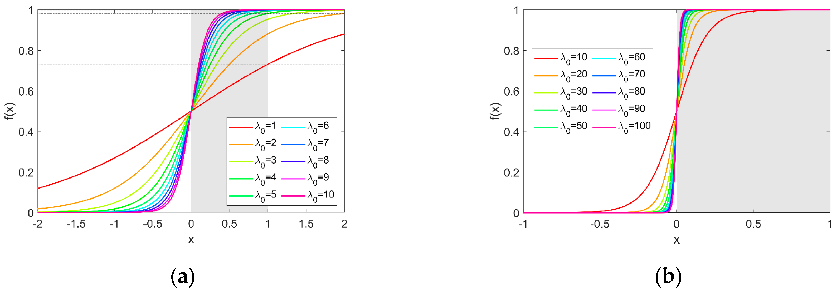
- FCM-O is proposed to overcome the causal inference error caused by non-linear mapping of the activation function. In FCM-O, the activation function is not used, and the offset is introduced to better train directed weighted graphs to illustrate the specific relationship between any pair of elements.
- (2)
- The FCM-O of ROO for the Three Gorges Reservoir (TGR) is established. The causal relationships between optimal control water level and inflow are inferred using FCM-O, and they are presented as intuitive graphical forms. In addition, some relevant conclusions are obtained.
2. Problem Formulation
2.1. Objective Function
2.2. Constraints
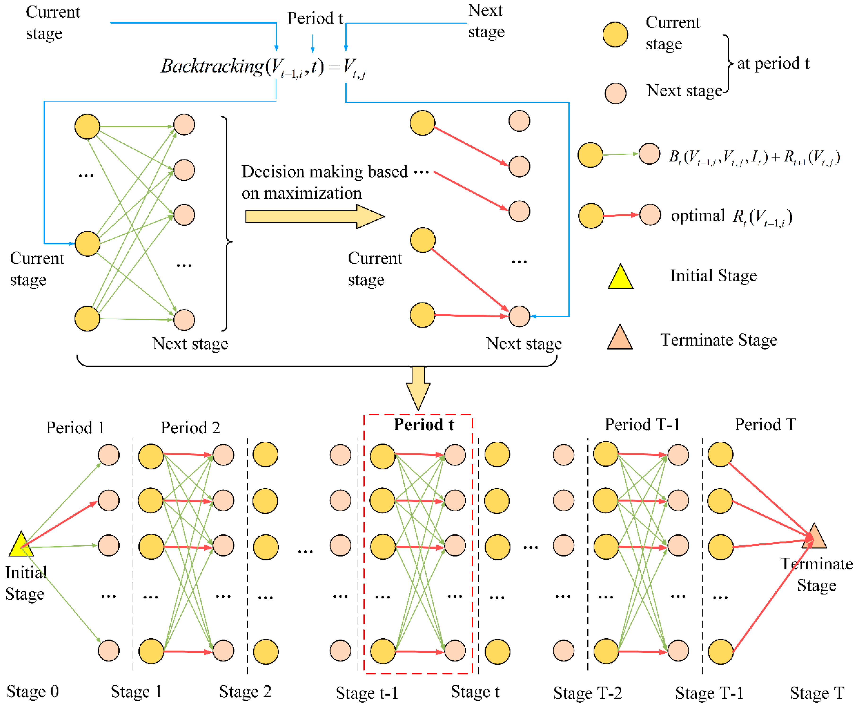
3. Obtaining the Optimal Control Water Level of Reservoir Optimal Operation Using Dynamic Programming
| Algorithm 1 DP for reservoir operation |
| Input: |
| 1: set Vbegin and Vend; select inflow series {It}. |
| Initialization: |
| 1: the states (reservoir capacity) are discretized |
| 2: generate discrete set of states {} |
| Calculation: |
| 1: for t = T to 1 |
| 2: for i = 1 to n select state from {} |
| 3: select optimal decision from { } to obtain the optimal Rt() |
| 4: save the backtracking relationship Backtracking(, t) = |
| 5: end for |
| 6: end for |
| Output: |
| the optimal benefit R1(Vbegin) and optimal state (decision) process {} |
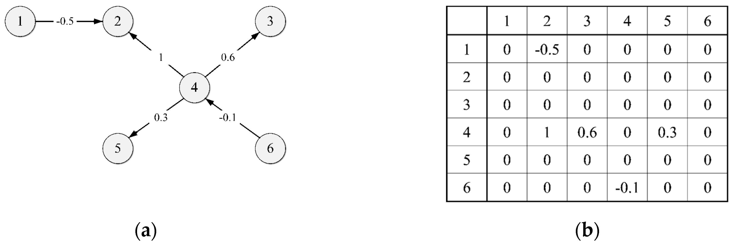
4. Fuzzy Cognitive Map with Offset
4.1. Fuzzy Cognitive Map
4.2. Fuzzy Cognitive Map with Offset
4.3. Algorithm for Learning the Structure of FCM: Differential Evolution Algorithm
5. Case Study
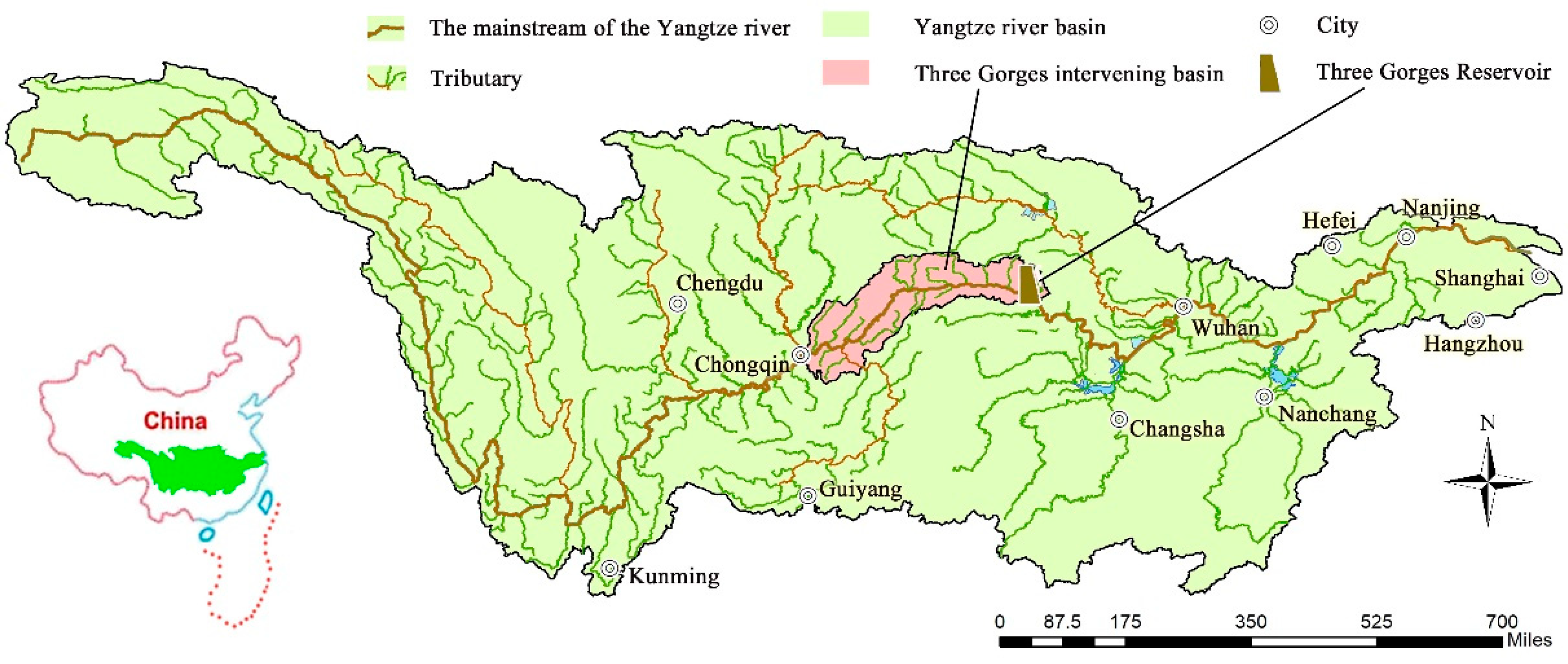
5.1. Description of Research Area
5.2. Dataset Acquisition and Preprocessing
- (1)
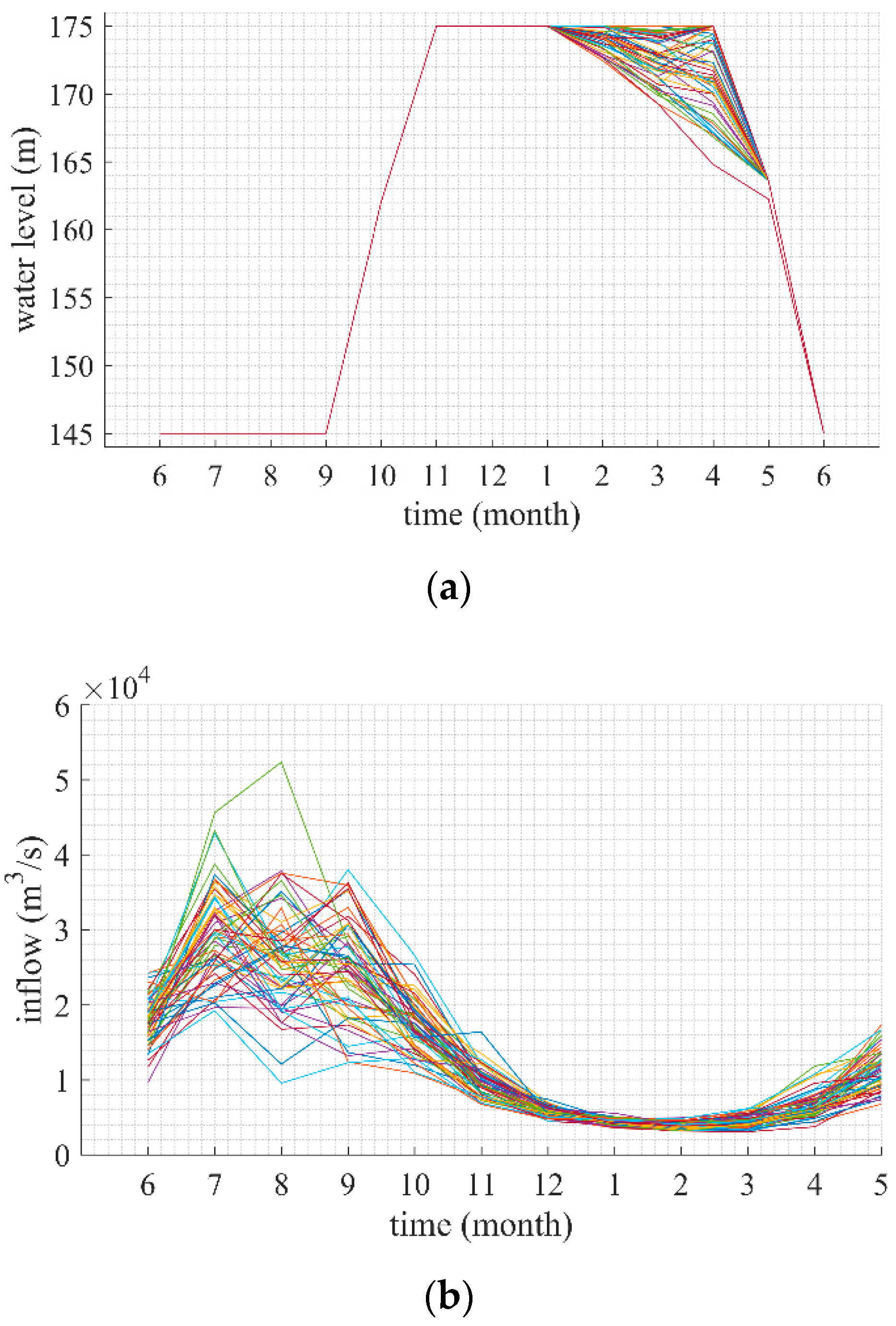
- For power generation, the water level of TGR should be higher than 145 m, which is the dead water level. In addition, TGR should keep lower than the normal water level 175 m.
- (2)
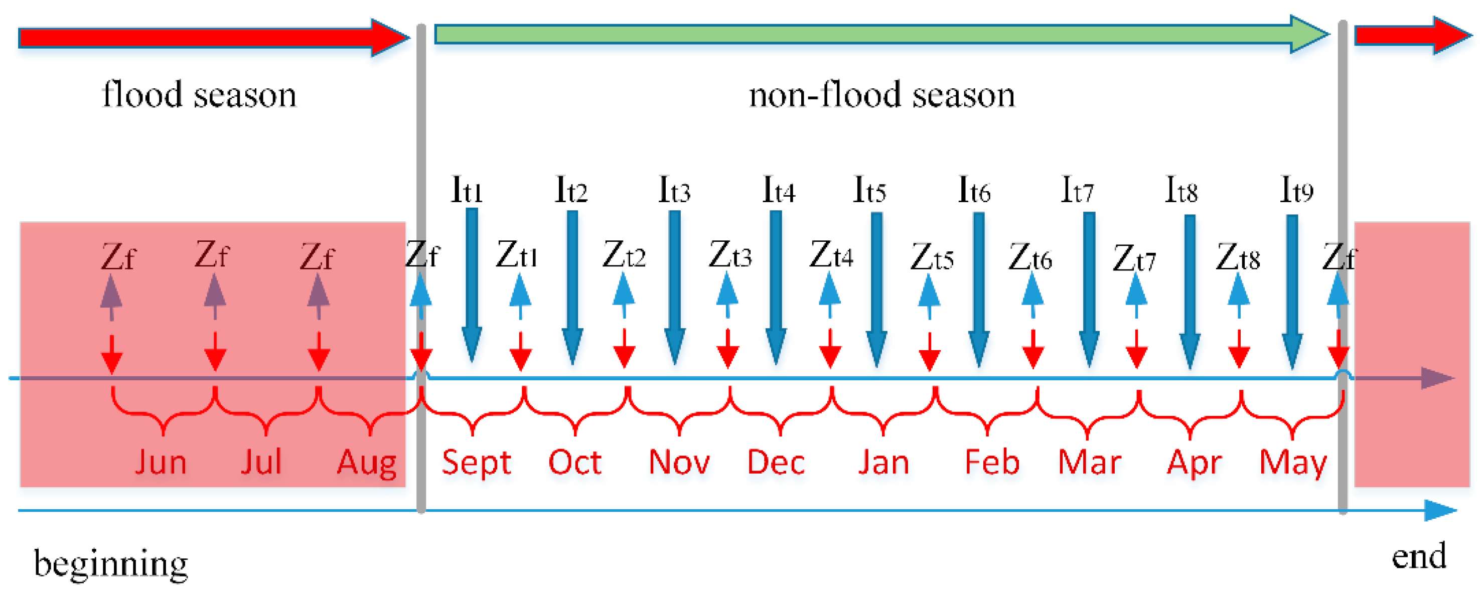
- From July to early September, the TGR runs according to the flood control mode.
- (3)
- TGR begins to store water in September, and reaches 175 m by late October. TGR had better fill up quickly to improve the efficiency of power generation.
5.3. Case Study and Discussion
6. Conclusions
Author Contributions
Funding
Acknowledgments
Conflicts of Interest
References
- Wang, H.; Yang, Z.; Saito, Y.; Liu, J.P.; Sun, X. Interannual and seasonal variation of the Huanghe (Yellow River) water discharge over the past 50 years: Connections to impacts from ENSO events and dams. Glob. Planet. Chang. 2006, 50, 212–225. [Google Scholar] [CrossRef]
- Feng, Z.; Niu, W.; Cheng, C. China’s large-scale hydropower system: Operation characteristics, modeling challenge and dimensionality reduction possibilities. Renew. Energy 2019, 136, 805–818. [Google Scholar] [CrossRef]
- Babel, M.S.; Dinh, C.N.; Mullick, M.R.A.; Nanduri, U.V. Operation of a hydropower system considering environmental flow requirements: A case study in La Nga river basin, Vietnam. J. Hydro-Environ. Res. 2012, 6, 63–73. [Google Scholar] [CrossRef]
- Feng, Z.K.; Niu, W.J.; Wang, W.C.; Zhou, J.Z.; Cheng, C.T. A mixed integer linear programming model for unit commitment of thermal plants with peak shaving operation aspect in regional power grid lack of flexible hydropower energy. Energy 2019, 175, 618–629. [Google Scholar] [CrossRef]
- Zhao, T.; Zhao, J.; Yang, D. Improved dynamic programming for hydropower reservoir operation. J. Water Resour. Plan. Manag. 2012, 140, 365–374. [Google Scholar] [CrossRef]
- Zhao, T.; Cai, X.; Lei, X.; Wang, H. Improved dynamic programming for reservoir operation optimization with a concave objective function. J. Water Resour. Plan. Manag. 2011, 138, 590–596. [Google Scholar] [CrossRef]
- He, Z.; Zhou, J.; Qin, H.; Jia, B.; Lu, C. Long-term joint scheduling of hydropower station group in the upper reaches of the Yangtze River using partition parameter adaptation differential evolution. Eng. Appl. Artif. Intell. 2019, 81, 1–13. [Google Scholar] [CrossRef]
- Liu, Y.; Qin, H.; Mo, L.; Wang, Y.; Chen, D.; Pang, S.; Yin, X. Hierarchical Flood Operation Rules Optimization Using Multi-Objective Cultured Evolutionary Algorithm Based on Decomposition. Water Resour. Manag. 2019, 33, 337–354. [Google Scholar] [CrossRef]
- Wang, Q.; Zhou, J.; Huang, K.; Dai, L.; Zha, G.; Chen, L.; Qin, H. Risk assessment and decision-making based on mean-CVaR-entropy for flood control operation of large scale reservoirs. Water 2019, 11, 649. [Google Scholar] [CrossRef]
- Huang, K.; Ye, L.; Chen, L.; Wang, Q.; Dai, L.; Zhou, J.; Singh, V.P.; Huang, M.; Zhang, J. Risk analysis of flood control reservoir operation considering multiple uncertainties. J. Hydrol. 2018, 565, 672–684. [Google Scholar] [CrossRef]
- Liu, P.; Li, L.; Guo, S.; Xiong, L.; Zhang, W.; Zhang, J.; Xu, C.Y. Optimal design of seasonal flood limited water levels and its application for the Three Gorges Reservoir. J. Hydrol. 2015, 527, 1045–1053. [Google Scholar] [CrossRef]
- Chen, D.; Chen, Q.; Leon, A.S.; Li, R. A Genetic Algorithm Parallel Strategy for Optimizing the Operation of Reservoir with Multiple Eco-environmental Objectives. Water Resour. Manag. 2016, 30, 2127–2142. [Google Scholar] [CrossRef]
- Giuliani, M.; Castelletti, A.; Pianosi, F.; Mason, E.; Reed, P.M. Curses, tradeoffs, and scalable management: Advancing evolutionary multiobjective direct policy search to improve water reservoir operations. J. Water Resour. Plan. Manag. 2015, 142, 4015050. [Google Scholar] [CrossRef]
- Feng, Z.; Niu, W.; Cheng, C. Optimization of hydropower reservoirs operation balancing generation benefit and ecological requirement with parallel multi-objective genetic algorithm. Energy 2018, 153, 706–718. [Google Scholar] [CrossRef]
- He, Z.; Zhou, J.; Mo, L.; Qin, H.; Xiao, X.; Jia, B.; Wang, C. Multiobjective reservoir operation optimization using improved multiobjective dynamic programming based on reference lines. IEEE Access 2019, 7, 103473–103484. [Google Scholar] [CrossRef]
- Bai, T.; Wei, J.; Chang, F.J.; Yang, W.; Huang, Q. Optimize multi-objective transformation rules of water-sediment regulation for cascade reservoirs in the Upper Yellow River of China. J. Hydrol. 2019, 577, 123987. [Google Scholar] [CrossRef]
- Tsai, W.P.; Chang, F.J.; Chang, L.C.; Herricks, E.E. AI techniques for optimizing multi-objective reservoir operation upon human and riverine ecosystem demands. J. Hydrol. 2015, 530, 634–644. [Google Scholar] [CrossRef]
- Chang, L.C.; Chang, F.J. Multi-objective evolutionary algorithm for operating parallel reservoir system. J. Hydrol. 2009, 377, 12–20. [Google Scholar] [CrossRef]
- Jiang, Z.; Qin, H.; Ji, C.; Hu, D.; Zhou, J. Effect Analysis of Operation Stage Difference on Energy Storage Operation Chart of Cascade Reservoirs. Water Resour. Manag. 2019, 33, 1349–1365. [Google Scholar] [CrossRef]
- Jiang, Z.; Qiao, Y.; Chen, Y.; Ji, C. A New Reservoir Operation Chart Drawing Method Based on Dynamic Programming. Energies 2018, 11, 3355. [Google Scholar] [CrossRef]
- Feng, Z.K.; Niu, W.J.; Zhang, R.; Wang, S.; Cheng, C.T. Operation rule derivation of hydropower reservoir by k-means clustering method and extreme learning machine based on particle swarm optimization. J. Hydrol. 2019, 576, 229–238. [Google Scholar] [CrossRef]
- Niu, W.J.; Feng, Z.K.; Feng, B.F.; Min, Y.W.; Cheng, C.T.; Zhou, J.Z. Comparison of multiple linear regression, artificial neural network, extreme learning machine, and support vector machine in deriving operation rule of hydropower reservoir. Water 2019, 11, 88. [Google Scholar] [CrossRef]
- Feng, M.; Liu, P.; Guo, S.; Gui, Z.; Zhang, X.; Zhang, W.; Xiong, L. Identifying changing patterns of reservoir operating rules under various inflow alteration scenarios. Adv. Water Resour. 2017, 104, 23–36. [Google Scholar] [CrossRef]
- Fu, W.; Wang, K.; Zhang, C.; Tan, J. A hybrid approach for measuring the vibrational trend of hydroelectric unit with enhanced multi-scale chaotic series analysis and optimized least squares support vector machine. Trans. Inst. Meas. Control 2019, 41, 4436–4449. [Google Scholar] [CrossRef]
- He, Z.; Zhou, J.; Sun, N.; Jia, B.; Qin, H. Integrated scheduling of hydro, thermal and wind power with spinning reserve. Energy Procedia 2019, 158, 6302–6308. [Google Scholar] [CrossRef]
- Chang, L.; Chang, F. Intelligent control for modelling of real-time reservoir operation. Hydrol. Process. 2001, 15, 1621–1634. [Google Scholar] [CrossRef]
- Jiang, Z.; Li, A.; Ji, C.; Qin, H.; Yu, S.; Li, Y. Research and application of key technologies in drawing energy storage operation chart by discriminant coefficient method. Energy 2016, 114, 774–786. [Google Scholar] [CrossRef]
- Yoo, J.H. Maximization of hydropower generation through the application of a linear programming model. J. Hydrol. 2009, 376, 182–187. [Google Scholar] [CrossRef]
- Catalão, J.P.; Pousinho, H.M.I.; Mendes, V.M.F. Scheduling of head-dependent cascaded hydro systems: Mixed-integer quadratic programming approach. Energy Convers. Manag. 2010, 51, 524–530. [Google Scholar] [CrossRef]
- Jiang, Z.; Qin, H.; Ji, C.; Feng, Z.; Zhou, J. Two dimension reduction methods for multi-dimensional dynamic programming and its application in cascade reservoirs operation optimization. Water 2017, 9, 634. [Google Scholar] [CrossRef]
- Nanda, J.; Bijwe, P.R. Optimal Hydrothermal Scheduling with Cascaded Plants Using Progressive Optimality Algorithm. IEEE Trans. Power Appar. Syst. 1981, PAS-100, 2093–2099. [Google Scholar] [CrossRef]
- Wang, C.; Zhou, J.; Lu, P.; Yuan, L. Long-term scheduling of large cascade hydropower stations in Jinsha River, China. Energy Convers. Manag. 2015, 90, 476–487. [Google Scholar] [CrossRef]
- Lee, J.; Labadie, J.W. Stochastic optimization of multireservoir systems via reinforcement learning. Water Resour. Res. 2007, 43, W11408. [Google Scholar] [CrossRef]
- Cheng, C.T.; Liao, S.L.; Tang, Z.T.; Zhao, M.Y. Comparison of particle swarm optimization and dynamic programming for large scale hydro unit load dispatch. Energy Convers. Manag. 2009, 50, 3007–3014. [Google Scholar] [CrossRef]
- Yuan, X.; Yuan, Y. Application of cultural algorithm to generation scheduling of hydrothermal systems. Energy Convers. Manag. 2006, 47, 2192–2201. [Google Scholar] [CrossRef]
- Arvanitidits, N.V.; Rosing, J. Composite representation of a multireservoir hydroelectric power system. IEEE Trans. Power Appar. Syst. 1970, PAS-89, 319–326. [Google Scholar] [CrossRef]
- Brandao, J.L.B. Performance of the equivalent reservoir modelling technique for multi-reservoir hydropower systems. Water Resour. Manag. 2010, 24, 3101–3114. [Google Scholar] [CrossRef]
- Zhao, T.; Zhao, J.; Liu, P.; Lei, X. Evaluating the marginal utility principle for long-term hydropower scheduling. Energy Convers. Manag. 2015, 106, 213–223. [Google Scholar] [CrossRef] [Green Version]
- Zhao, T.; Zhao, J.; Lei, X.; Wang, X.; Wu, B. Improved Dynamic Programming for Reservoir Flood Control Operation. Water Resour. Manag. 2017, 31, 2047–2063. [Google Scholar] [CrossRef]
- Kosko, B. Fuzzy cognitive maps. Int. J. Man Mach. Stud. 1986, 24, 65–75. [Google Scholar] [CrossRef]
- Papakostas, G.A.; Koulouriotis, D.E.; Polydoros, A.S.; Tourassis, V.D. Towards Hebbian learning of Fuzzy Cognitive Maps in pattern classification problems. Expert Syst. Appl. 2012, 39, 10620–10629. [Google Scholar] [CrossRef]
- Papageorgiou, E.; Stylios, C.; Groumpos, P. Fuzzy cognitive map learning based on nonlinear Hebbian rule. In Proceedings of the Australasian Joint Conference on Artificial Intelligence, Perth, WA, Australia, 3–5 December 2003; pp. 256–268. [Google Scholar]
- Salmeron, J.L.; Mansouri, T.; Moghadam, M.R.S.; Mardani, A. Learning Fuzzy Cognitive Maps with modified asexual reproduction optimisation algorithm. Knowl. Based Syst. 2019, 163, 723–735. [Google Scholar] [CrossRef]
- Poczeta, K.; Kubuś, Ł.; Yastrebov, A. Analysis of an evolutionary algorithm for complex fuzzy cognitive map learning based on graph theory metrics and output concepts. Biosystems 2019, 179, 39–47. [Google Scholar] [CrossRef] [PubMed]
- Chen, Y.; Mazlack, L.J.; Minai, A.A.; Lu, L.J. Inferring causal networks using fuzzy cognitive maps and evolutionary algorithms with application to gene regulatory network reconstruction. Appl. Soft Comput. 2015, 37, 667–679. [Google Scholar] [CrossRef]
- Mendonça, M.; Angelico, B.; Arruda, L.V.R.; Neves, F., Jr. A dynamic fuzzy cognitive map applied to chemical process supervision. Eng. Appl. Artif. Intell. 2013, 26, 1199–1210. [Google Scholar] [CrossRef]
- Stylios, C.D.; Groumpos, P.P. Modeling complex systems using fuzzy cognitive maps. IEEE Trans. Syst. Man Cybern. Part A Syst. Hum. 2004, 34, 155–162. [Google Scholar] [CrossRef]
- Hossain, S.; Brooks, L. Fuzzy cognitive map modelling educational software adoption. Comput. Educ. 2008, 51, 1569–1588. [Google Scholar] [CrossRef]
- Kok, K. The potential of Fuzzy Cognitive Maps for semi-quantitative scenario development, with an example from Brazil. Glob. Environ. Chang. 2009, 19, 122–133. [Google Scholar] [CrossRef]
- Zhang, K.; Pan, Q.; Yu, D.; Wang, L.; Liu, Z.; Li, X.; Liu, X. Systemically modeling the relationship between climate change and wheat aphid abundance. Sci. Total Environ. 2019, 674, 392–400. [Google Scholar] [CrossRef]
- Wen, X.; Zhou, J.; He, Z.; Wang, C. Long-term scheduling of large-scale cascade hydropower stations using improved differential evolution algorithm. Water 2018, 10, 383. [Google Scholar] [CrossRef]
- Bellman, R.E.; Dreyfus, S.E. Applied Dynamic Programming; Princeton University Press: Princeton, NJ, USA, 2015; Volume 2050, ISBN 1400874653. [Google Scholar]
- Yakowitz, S. Dynamic programming applications in water resources. Water Resour. Res. 1982, 18, 673–696. [Google Scholar] [CrossRef]
- Labadie, J.W. Optimal operation of multireservoir systems: State-of-the-art review. J. Water Resour. Plan. Manag. 2004, 130, 93–111. [Google Scholar] [CrossRef]
- Loucks, D.P.; Van Beek, E.; Stedinger, J.R.; Dijkman, J.P.M.; Villars, M.T. Water Resources Systems Planning and Management: An Introduction to Methods, Models and Applications; Unesco: Paris, France, 2005; ISBN 9231039989. [Google Scholar]
- Wu, K.; Liu, J. Robust learning of large-scale fuzzy cognitive maps via the lasso from noisy time series. Knowl. Based Syst. 2016, 113, 23–38. [Google Scholar] [CrossRef]
- Tsadiras, A.K. Comparing the inference capabilities of binary, trivalent and sigmoid fuzzy cognitive maps. Inf. Sci. 2008, 178, 3880–3894. [Google Scholar] [CrossRef]
- Bueno, S.; Salmeron, J.L. Benchmarking main activation functions in fuzzy cognitive maps. Expert Syst. Appl. 2009, 36, 5221–5229. [Google Scholar] [CrossRef]
- Stach, W.; Pedrycz, W.; Kurgan, L.A. Learning of fuzzy cognitive maps using density estimate. IEEE Trans. Syst. Man Cybern. Part B (Cybern.) 2012, 42, 900–912. [Google Scholar] [CrossRef] [PubMed]
- Chen, Y.; Mazlack, L.; Lu, L. Learning fuzzy cognitive maps from data by ant colony optimization. In Proceedings of the 14th Annual Conference on Genetic and Evolutionary Computation, Philadelphia, PA, USA, 7–11 July 2012; pp. 9–16. [Google Scholar]
- Papageorgiou, E.I. Learning algorithms for fuzzy cognitive maps—A review study. IEEE Trans. Syst. Man Cybern. Part C (Appl. Rev.) 2011, 42, 150–163. [Google Scholar] [CrossRef]
- Stach, W.; Kurgan, L.; Pedrycz, W. A divide and conquer method for learning large fuzzy cognitive maps. Fuzzy Sets Syst. 2010, 161, 2515–2532. [Google Scholar] [CrossRef]
- Stach, W.; Kurgan, L.; Pedrycz, W.; Reformat, M. Evolutionary development of fuzzy cognitive maps. In Proceedings of the The 14th IEEE International Conference on Fuzzy Systems, Reno, NV, USA, 25 May 2005; pp. 619–624. [Google Scholar]
- Das, S.; Suganthan, P.N. Differential evolution: A survey of the state-of-the-art. IEEE Trans. Evol. Comput. 2011, 15, 4–31. [Google Scholar] [CrossRef]
- Storn, R.; Price, K. Differential Evolution—A Simple and Efficient Heuristic for global Optimization over Continuous Spaces. J. Glob. Optim. 1997, 11, 341–359. [Google Scholar] [CrossRef]
- Li, J.Q.; Sang, H.Y.; Han, Y.Y.; Wang, C.G.; Gao, K.Z. Efficient multi-objective optimization algorithm for hybrid flow shop scheduling problems with setup energy consumptions. J. Clean. Prod. 2018, 181, 584–598. [Google Scholar] [CrossRef]
- Tey, K.S.; Mekhilef, S.; Seyedmahmoudian, M.; Horan, B.; Oo, A.T.; Stojcevski, A. Improved differential evolution-based MPPT algorithm using SEPIC for PV systems under partial shading conditions and load variation. IEEE Trans. Ind. Inform. 2018, 14, 4322–4333. [Google Scholar] [CrossRef]
- Tanabe, R.; Fukunaga, A.S. Improving the search performance of SHADE using linear population size reduction. In Proceedings of the Evolutionary Computation, Beijing, China, 6–11 July 2014; pp. 1658–1665. [Google Scholar]
- Zhang, J.; Sanderson, A.C. JADE: Adaptive Differential Evolution With Optional External Archive. IEEE Trans. Evol. Comput. 2009, 13, 945–958. [Google Scholar] [CrossRef]
- Tanabe, R.; Fukunaga, A. Success-history based parameter adaptation for Differential Evolution. In Proceedings of the Evolutionary Computation, Cancun, Mexico, 20–23 June 2013; pp. 71–78. [Google Scholar]
- Liang, J.J.; Qu, B.Y.; Suganthan, P.N. Problem Definitions and Evaluation Criteria for the CEC 2014 Special Session and Competition on Single Objective Real-Parameter Numerical Optimization; Technical Report 201311; Zhengzhou University and Nanyang Technological University: Singapore, 2013. [Google Scholar]
- Piotrowski, A.P.; Napiorkowski, J.J. Step-by-step improvement of JADE and SHADE-based algorithms: Success or failure? Swarm Evol. Comput. 2018, 43, 88–108. [Google Scholar] [CrossRef]
- Peng, F.; Tang, K.; Chen, G.; Yao, X. Multi-start JADE with knowledge transfer for numerical optimization. In Proceedings of the Eleventh Conference on Congress on Evolutionary Computation, Trondheim, Norway, 18–21 May 2009; pp. 1889–1895. [Google Scholar]
- Zhou, J.; Xie, M.; He, Z.; Qin, H.; Yuan, L. Medium-Term Hydro Generation Scheduling (MTHGS) with Chance Constrained Model (CCM) and Dynamic Control Model (DCM). Water Resour. Manag. 2017, 31, 3543–3555. [Google Scholar] [CrossRef]


| Parameter | TGR |
|---|---|
| Adjustment ability | Season |
| Total reservoir capacity (billion m3) | 39.30 |
| Regulating storage (billion m3) | 16.50 |
| Hydro plant discharge range(m3/s) | (98, 800, 4500) |
| Upriver water level range (m) | (175, 145) |
| Installed capacity (MW) | 22,400 |
| Normal water level (m) | 175 |
| Maximum water level amplitude(m/d) | 0.6 |
| t | t1 | ||||||||
| month | 9 | 10 | 11 | 12 | 1 | 2 | 3 | 4 | 5 |
| Sept | Oct | Nov | Dec | Jan | Feb | Mar | Apr | May |
| Method | Training | Testing | |
|---|---|---|---|
| min data error | FCM | 0.0045 | 0.0056 |
| FCM-O | 0.0040 | 0.0052 | |
| FCM-O vs. FCM in the reduction of min data error | 11.11% | 7.14% | |
| Z9 | Z10 | Z11 | Z12 | Z1 | Z2 | Z3 | Z4 | |
|---|---|---|---|---|---|---|---|---|
| I9 | −1.00 | 1.00 | 1.00 | 1.00 | 0.20 | −0.03 | −0.30 | −0.24 |
| I10 | −1.00 | 1.00 | 1.00 | 1.00 | −0.09 | −0.13 | −0.07 | −0.16 |
| I11 | −1.00 | 1.00 | 1.00 | 1.00 | 1.00 | 1.00 | 0.72 | −0.16 |
| I12 | −1.00 | 1.00 | 1.00 | 1.00 | 1.00 | 0.62 | 0.79 | −0.40 |
| I1 | −1.00 | 1.00 | 1.00 | 1.00 | 1.00 | 1.00 | 1.00 | −1.00 |
| I2 | −1.00 | 1.00 | 1.00 | 1.00 | 1.00 | 1.00 | 1.00 | 0.36 |
| I3 | −1.00 | 1.00 | 1.00 | 1.00 | 1.00 | 1.00 | 1.00 | −1.00 |
| I4 | −1.00 | 1.00 | 1.00 | 1.00 | 1.00 | 1.00 | 1.00 | 0.09 |
| I5 | −1.00 | 1.00 | 1.00 | 1.00 | 0.01 | −0.29 | 0.10 | −0.34 |
| λ0 | 5.00 | 5.00 | 5.00 | 5.00 | 5.00 | 5.00 | 5.00 | 5.00 |
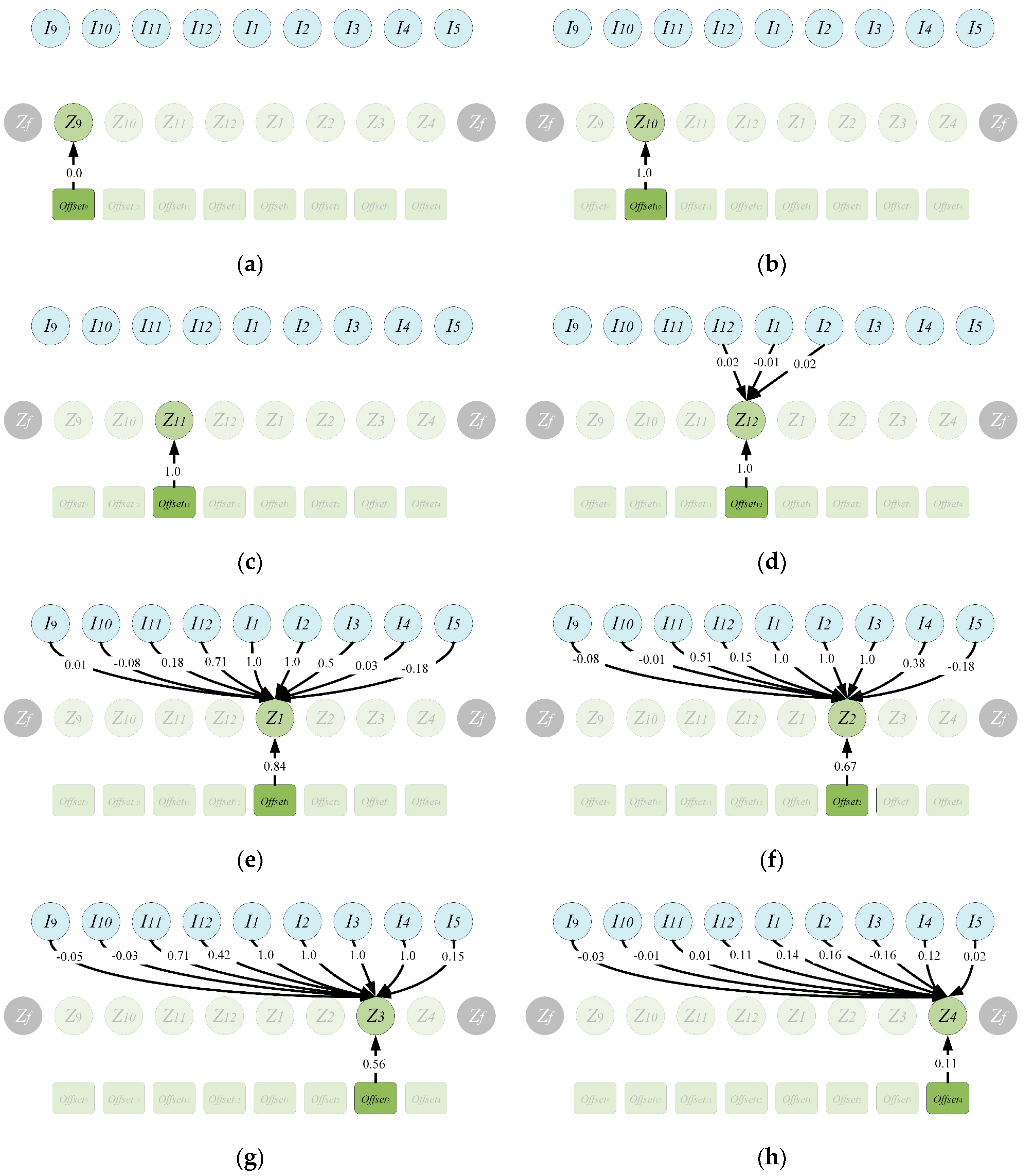
| Z9 | Z10 | Z11 | Z12 | Z1 | Z2 | Z3 | Z4 | |
|---|---|---|---|---|---|---|---|---|
| I9 | 0.00 | 0.00 | 0.00 | 0.00 | 0.01 | −0.08 | −0.05 | −0.03 |
| I10 | 0.00 | 0.00 | 0.00 | 0.00 | −0.08 | −0.01 | −0.03 | −0.01 |
| I11 | 0.00 | 0.00 | 0.00 | 0.00 | 0.18 | 0.51 | 0.71 | 0.01 |
| I12 | 0.00 | 0.00 | 0.00 | 0.02 | 0.71 | 0.15 | 0.42 | 0.11 |
| I1 | 0.00 | 0.00 | 0.00 | −0.01 | 1.00 | 1.00 | 1.00 | 0.14 |
| I2 | 0.00 | 0.00 | 0.00 | 0.02 | 1.00 | 1.00 | 1.00 | 0.16 |
| I3 | 0.00 | 0.00 | 0.00 | 0.00 | 0.50 | 1.00 | 1.00 | −0.16 |
| I4 | 0.00 | 0.00 | 0.00 | 0.00 | 0.03 | 0.38 | 1.00 | 0.12 |
| I5 | 0.00 | 0.00 | 0.00 | 0.00 | −0.18 | −0.18 | 0.15 | 0.02 |
| 0.00 | 1.00 | 1.00 | 1.00 | 0.84 | 0.67 | 0.56 | 0.11 |
| In Degree | In Element | ||
|---|---|---|---|
| Z9 | 0 | 0 | |
| Z10 | 0 | 1 | |
| Z11 | 0 | 1 | |
| Z12 | 3 | I12, I1, I2 | 1 |
| Z1 | 9 | I9, I10, I11, I12, I1, I2, I3, I4, I5 | 0.84 |
| Z2 | 9 | I9, I10, I11, I12, I1, I2, I3, I4, I5 | 0.67 |
| Z3 | 9 | I9, I10, I11, I12, I1, I2, I3, I4, I5 | 0.56 |
| Z4 | 9 | I9, I10, I11, I12, I1, I2, I3, I4, I5 | 0.11 |
© 2019 by the authors. Licensee MDPI, Basel, Switzerland. This article is an open access article distributed under the terms and conditions of the Creative Commons Attribution (CC BY) license (http://creativecommons.org/licenses/by/4.0/).
Share and Cite
Liu, Y.; Zhou, J.; He, Z.; Lu, C.; Jia, B.; Qin, H.; Feng, K.; He, F.; Liu, G. Causal Inference of Optimal Control Water Level and Inflow in Reservoir Optimal Operation Using Fuzzy Cognitive Map. Water 2019, 11, 2147. https://doi.org/10.3390/w11102147
Liu Y, Zhou J, He Z, Lu C, Jia B, Qin H, Feng K, He F, Liu G. Causal Inference of Optimal Control Water Level and Inflow in Reservoir Optimal Operation Using Fuzzy Cognitive Map. Water. 2019; 11(10):2147. https://doi.org/10.3390/w11102147
Chicago/Turabian StyleLiu, Yi, Jianzhong Zhou, Zhongzheng He, Chengwei Lu, Benjun Jia, Hui Qin, Kuaile Feng, Feifei He, and Guangbiao Liu. 2019. "Causal Inference of Optimal Control Water Level and Inflow in Reservoir Optimal Operation Using Fuzzy Cognitive Map" Water 11, no. 10: 2147. https://doi.org/10.3390/w11102147