Simulating the Impact of Climate Change on the Hydrological Regimes of a Sparsely Gauged Mountainous Basin, Northern Pakistan


1
Institute of Hydrology and Meteorology, Technische Universität Dresden, 01062 Dresden, Germany
2
Department of Remote Sensing Am Hubland, Institute of Geography and Geology, University of Wurzburg, 97080 Würzburg, Germany
3
Department of Irrigation and Drainage, University of Agriculture, Faisalabad 38000, Pakistan
*
Author to whom correspondence should be addressed.
Water 2019, 11(10), 2141; https://doi.org/10.3390/w11102141
Submission received: 18 September 2019
/
Revised: 11 October 2019
/
Accepted: 12 October 2019
/
Published: 15 October 2019
(This article belongs to the Section Hydrology)
Abstract
:Projected climate changes for the 21st century may cause great uncertainties on the hydrology of a river basin. This study explored the impacts of climate change on the water balance and hydrological regime of the Jhelum River Basin using the Soil and Water Assessment Tool (SWAT). Two downscaling methods (SDSM, Statistical Downscaling Model and LARS-WG, Long Ashton Research Station Weather Generator), three Global Circulation Models (GCMs), and two representative concentration pathways (RCP4.5 and RCP8.5) for three future periods (2030s, 2050s, and 2090s) were used to assess the climate change impacts on flow regimes. The results exhibited that both downscaling methods suggested an increase in annual streamflow over the river basin. There is generally an increasing trend of winter and autumn discharge, whereas it is complicated for summer and spring to conclude if the trend is increasing or decreasing depending on the downscaling methods. Therefore, the uncertainty associated with the downscaling of climate simulation needs to consider, for the best estimate, the impact of climate change, with its uncertainty, on a particular basin. The study also resulted that water yield and evapotranspiration in the eastern part of the basin (sub-basins at high elevation) would be most affected by climate change. The outcomes of this study would be useful for providing guidance in water management and planning for the river basin under climate change.
1. Introduction
The fifth assessment report of the Intergovernmental Panel on Climate Change (IPCC, AR5) points out that the earth air temperature has increased by 0.85 °C for 1881–2012 and for each of the recent past three decades. More temperature has been recorded for every consecutive decade. More specifically, it has been projected that the mean temperature will increase over 1 °C under the low emission scenario (RCP2.6) and over 4 °C under the high emission scenario (RCP8.5) [1]. In many studies, an increasing temperature trend has been observed in the Himalayan basins [2,3,4]. For instance, a study conducted by Immerzeel et al. in the Himalayas catchment concluded that the availability of water in the 21st century is not likely to decrease due to the rise in glacier melt and increasing rainfall [5].
The most often used method for impact assessment of climate change on hydrological cycles is by forcing the outputs of Global Circulation Models (GCMs) into hydrological models [6]. Generally, an ensemble approach of different GCMs, which could show various scenarios, is recommended that provide a better foresight into future climate than just using single GCM [7]. Many studies have utilized climate projections using an ensemble approach employing three to six GCMs [8,9,10,11]. Nevertheless, GCMs have a very coarse spatial resolution, which makes it inconsistent with the hydrological boundaries of the models. To fill this gap, the statistical or dynamical downscaling method can be involved as a bridge.
Uncertainties associated with the impact of climate change on hydrological regimes may arise from each of these four processes: GCMs, climate change scenarios, downscaling methods, and hydrological simulations. For instance, according to Chen et al., impact studies based on a single downscaling approach should be carefully assessed due to associated output uncertainties [12]. Wilby and Haris found that the more uncertainties emerge from the choice of GCMs and downscaling methods than the selection of hydrological models and climate scenarios [13]. Meaurio et al. concluded that the downscaling methods result in higher uncertainty than GCMs itself [14]. The uncertainty of hydrological models is cumulative as the inherent uncertainties of the downscaling methods used at each level keep on propagating to the next level and finally to the ultimate hydrological output [15].
For the simulation of future water cycles, hydrological models are used, GCMs project precipitation, and temperature data are used to force these models. The selection of the most suitable hydrological model to be employed depends on the spatial scale of the model, characteristics of basin, data availability, required accuracy and the objective of the study, and the ease of calibration [16]. The efficiency of the hydrological models is less in high-elevated and scarcely gauged basins, where snowmelt is a substantial part of water flow [17]. Therefore, it is quite challenging to estimate the runoff in such catchments.
The Soil and Water Assessment Tool (SWAT) is a physically-based, semi-distributed hydrologic model, which has been proved to be an effective tool for assessing the climate change impacts on water resources, and non-point source pollution problems for a wide range of spatial-temporal scales and ecosystems across the entire globe [18]. For example, Perazzoli et al. concluded the climate change impacts on the river flow changes and sediment production in a river basin located in southern Brazil [19]. Shi et al. analyzed the changes in land-use and climate and assessed their effects on the Huai River in China [20]. Yin et al. applied the Coupled Model Intercomparison Project 5 (CMIP5) model’s outputs and SWAT to project the impacts of climate change on the Jinsha River Basin [21]. They observed a decrease in streamflow by 2% to 5% in response to a 1 °C rise in temperature. Furthermore, Bajracharya et al. quantified the impact of climate change on the hydrological regime and water balance using the SWAT model under Representative Concentration Pathways (RCPs) scenarios [7]. The results showed that water balance components (water yield, snowmelt, and evapotranspiration) would be affected by climate change.
The overall objective of the current study was to disintegrate the contribution of precipitation, snowmelt, and evapotranspiration for water yield, considering the water balance of the Jhelum River Basin. It is all valuable to understand the impact of future hydro-climatic variability due to its importance for flood management and energy production. Previous studies had mainly focused only on the impact of climate change on streamflow, often ignoring other water balance components [22]. The most notable objectives of this study were: (i) to calibrate and validate the SWAT for simulating daily streamflow in the basin using snow parameters at sub-basin scale, (ii) projecting future precipitation and temperature from the data of three GCMs by using SDSM (Statistical Downscaling Model) and LARS-WG (Long Ashton Research Station Weather Generator), (iii) to analyze uncertainties in streamflow results obtained under different climate scenarios, and (iv) to quantify the impacts of future climate projections on the basin’s water balance components.
2. Study Area
Description of the Study Area
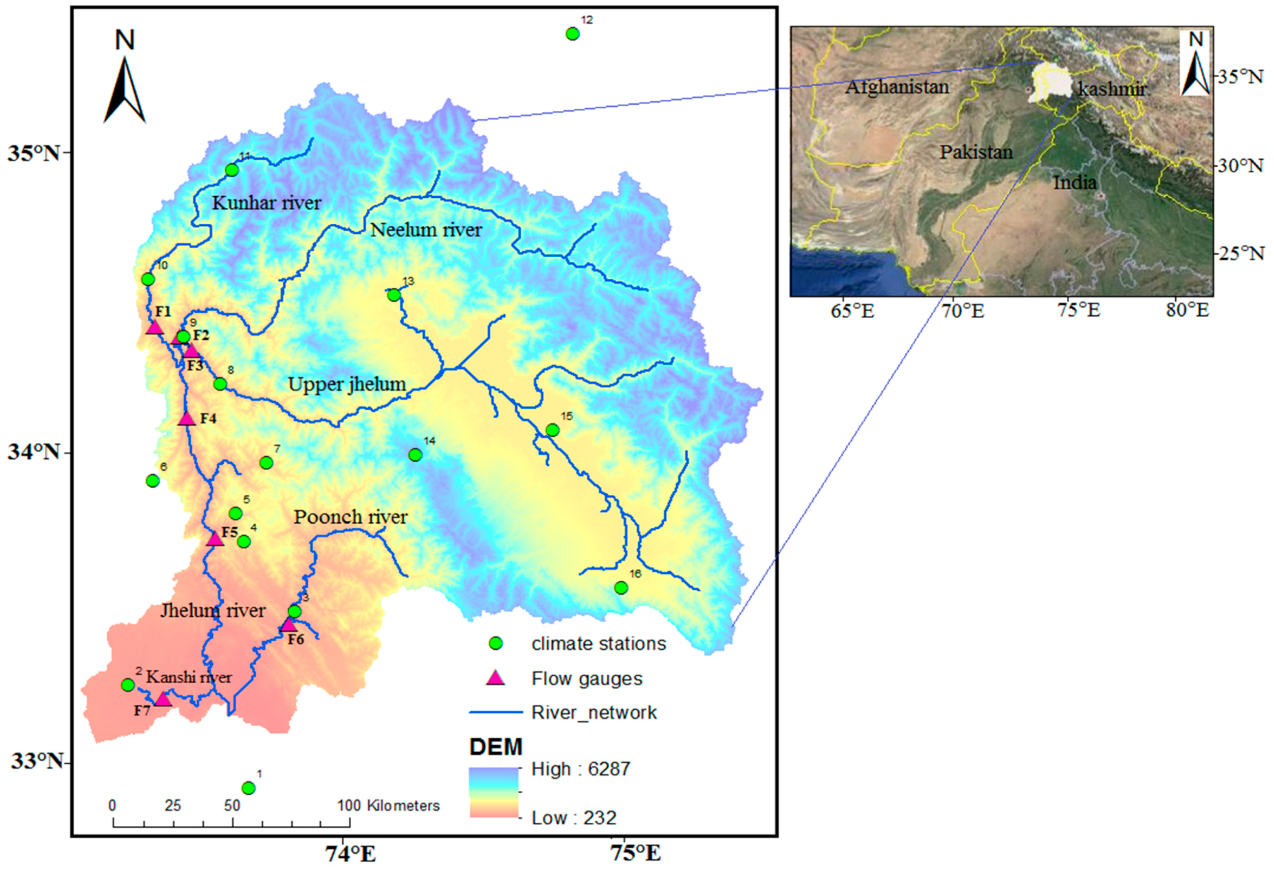
The Jhelum River Basin (JRB) (33,397 Km2) is a principal tributary of the Indus Basin after the Indus River. The JRB is around 725 km long and lying between 73–75.62 °E and 33–35 °N. The elevation stretches from 232 m to 6287 m with permanent snow-capped mountains in the north. The Kunhar, Neelum, and Poonch are three main tributaries of JRB. The basin drains its water in the Mangla reservoir, the country’s second-largest reservoir. More than 75% of the water flows to the reservoir from March to August. Mangla reservoir has a total command area of 6 Mha, and it serves two key purposes: supply water to irrigate the agricultural land and contribute 6% share in total electricity generation of the country [23].
It is very common to have a low-density network of climatic stations in developing countries like Pakistan. Due to the very complex topography of JRB, there are only 16 meteorological stations (Figure 1). The basin’s annual average maximum temperature is 30.8 °C (June and July), and the mean minimum temperature is 0.3 °C (December and January). The extremely cold station of the basin is Naran, where average air temperature goes below 0 °C in the winter season and does not exceed 16 °C in summer. The mean annual precipitation of the basin is about 1196 mm/year from 1961 to 2012 [24]. The annual mean runoff of JRB at Azad Pattan is 833 m3/s that is calculated from 1976 to 2005 (Table 1). The maximum discharge at Azad Pattan is 1741 m3/s, which occurs in June, while the minimum runoff is 223 m3/s, which happens in January.
3. Data Description
3.1. Hydro-Metrological Data
Table 2 gives the geographic and basic information of meteorological stations. The measured daily data of precipitation, maximum and minimum temperature were acquired from the Pakistan Meteorological Department (PMD), Water and Power Development Authority (WAPDA) of Pakistan, and the India Meteorological Department (IMD). The hydrological data of seven stations were obtained from the WAPDA (Table 1). All hydrological and meteorological data are available on a daily time scale.
3.2. Digital Elevation Data
The topography is an integral part of hydrological studies and is employed for watershed delineation, analysis of topographical features, and exploring drainage patterns [25,26]. It influences the movement rate and flow direction over the land surface [27]. In the present study, Digital Elevation Model (DEM) from the Shuttle Radar Topography Mission (SRTM) of National Aeronautics and Space Administration (NASA) with 30 m spatial resolution was used.
3.3. Land-Use and Soil Data
The land cover map was generated from the 30 m resolution Landsat 7 Enhanced Thematic Mapper (+ETM) data acquired in 2001. For the Land use/land cover (LULC) classification, the Random Forest machine learning algorithm in R language was applied to classify the image into five major classes, including agriculture, forest, grass, settlement, and water. Principle land-use in JRB is grass-sparse vegetation (36.79%) followed by agriculture (30.81%), forest (27.88%), settlement (2.43%), and water (2.07%), which are shown in Figure 2a.
Figure 2b provides the soil map of the study area. The soil data were obtained from the Food and Agriculture Organization (FAO) of the United Nations Harmonized World Soil Database (HWSD). The HWSD is a 30 arc-second raster database with over 15,000 different soil-mapping units. Eleven different types of soils are present in JRB, which are shown in Table 3. Gleyic Solonacks (covers about 49% of the basin area) is found in the high mountainous areas, Calaric Phaoeozems soil (covers almost 23% of the basin area) is found in the middle ranges, and Mollic Planosols soil (covers about 21% of the basin area) is in the northern valley areas.
3.4. Representative Concentration Pathway (RCPs) Scenarios
Four RCPs scenarios, namely 2.6, 4.5, 6.5, and 8.5, are defined based on different radiative forcing (2.6 to 8.5 Watt/m2). These radiative forcing levels depend on the emission of carbon dioxide. For the current study, we chose two RCPs (4.5 and 8.5). These two RCPs scenarios have been extensively used in climate change impact studies [7,11,14,28]. RCP4.5 and RCP8.5 correspond to the Special Report on Emissions Scenarios (SRES) B1 and A1F1 in terms of temperature anomaly. Three GCM (i.e., MIROC5, BCC-CSM1.1, and CanESM2) were selected from the literature review based on their performance and have been used widely in climate change studies in South Asia [29,30,31]. Table A1 provides the detail description (development countries, spatial resolution, and time) of all the GCMs used in this study.
Generally, GCMs outputs have a coarse resolution; such data cannot be directly used in SWAT and thus needs downscaling to fit the required finer resolution. Finer resolution can be achieved by using two types of techniques: (1) dynamical downscaling and (2) statistical downscaling. In this study, two statistical downscaling models were used - the Statistical Downscaling Model (SDSM), which uses multiple linear regression and other statistical relations between GSMs and existing weather station data, and the Long Ashton Research Station Weather Generator (LARS-WG), which uses a combination of GCM output and local weather station statistics. Daily climatic data (Tmax, Tmin, and Prec) were downscaled with SDSM and LARS-WG for the period 2006–2100. Different descriptive statistics, such as R2, PBIAS, Standard Deviation (SD), mean and Normalized Root Mean Square Error (NRMSE), were used to check the suitability of the GCMs data in the study area [24].
4. Methodology
4.1. Hydrological Modeling
SWAT is a semi-distributed hydrological model used to simulate the quality and quantity of water for different climate regimes and to assess the potential impacts of land-use, climate change, and land management practices on surface and groundwater. In the SWAT model, the whole catchment is divided into sub-basins, and a sub-basin further delineated into multiple Hydrological Response Units (HRUs) that consist of homogeneous land-use, soil, and topography. The water balance equation (1) given by Neitsch et al. [18] is involved in simulating the hydrological cycle.
where,
SWt; final soil water content (mmH2O)
SWo; initial soil water content (mmH2O)
t; time (days)
Rday; the amount of precipitation on the day i (mmH2O)
Qsurf; the amount of surface run-off (mmH2O)
Ea; the amount of evapotranspiration (mmH2O)
Wseep; the amount of water entering the vadose zone from the soil profile (mmH2O)
Qgw; the amount of baseflow (mmH2O)
SWAT distinguish precipitation as snow or rain by the values of the daily temperature. The snowmelt in the SWAT model is a linear function of the difference between the average snow pack’s maximum air temperature and the base or threshold temperature for snowmelt [18]. The snowmelt on a given day is represented by the following Equation (2),
where,
SNOWmelt; the amount of snowmelt (mm)
bmelt; melt factor
snowcov; the fraction of the HRU covered by snow
Tsnow; snowpack temperature (°C)
Tmax; maximum air temperature (°C)
Tmelt; base temperature above which snowmelt (°C)
The SWAT theoretical documentation [18] presents the individual components of the model: (a) Soil Conservation Service (SCS) curve number is employed to calculate the surface runoff, (b) the rate and velocity of overland in channel is obtained using Manning equation, and (c) lateral flow is simulated by kinematic storage model. For the estimation of evapotranspiration (ET), the Hargreaves method was employed because the wind speed, relative humidity, and solar radiation data were not available for the future.
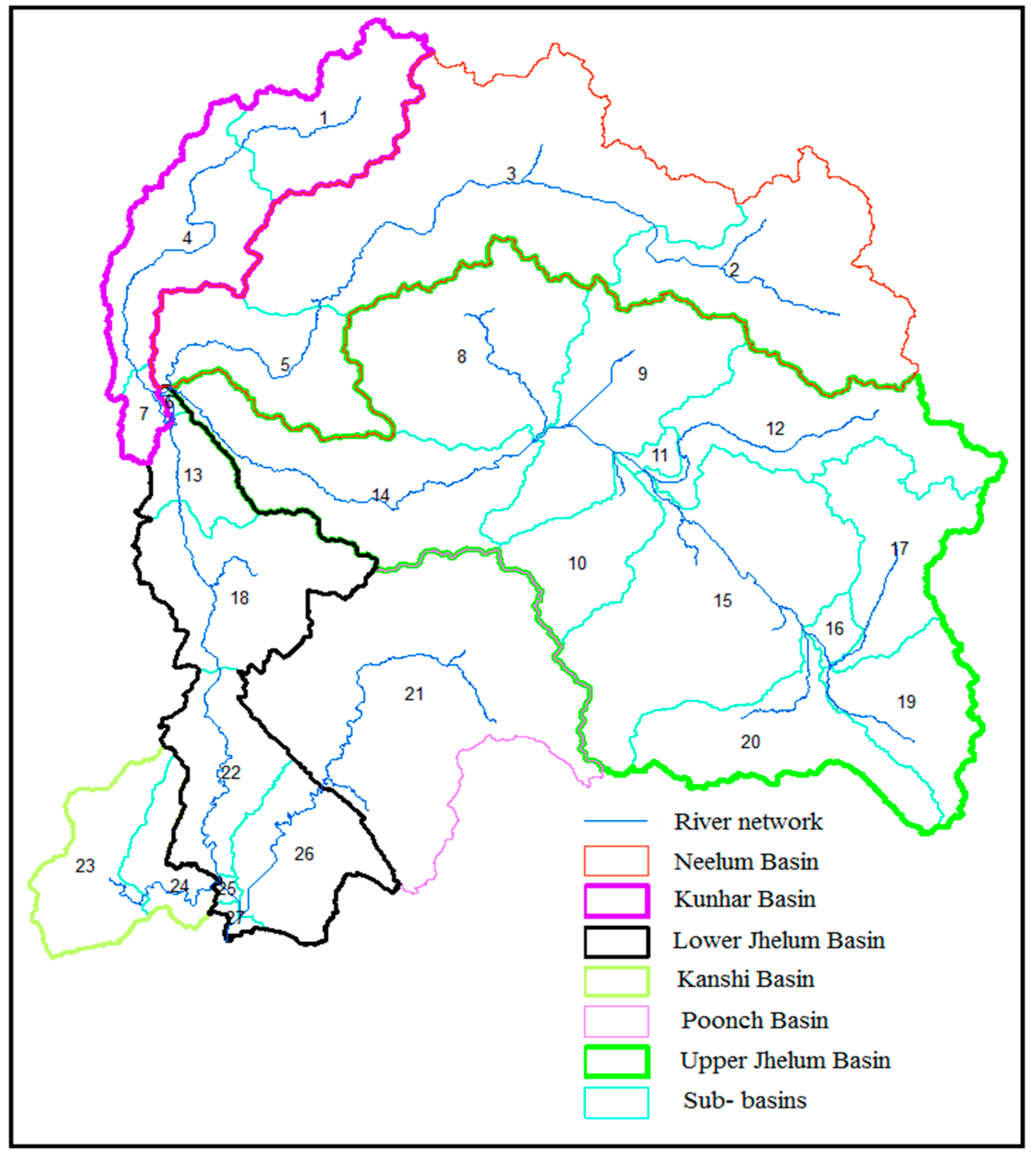
The Arc SWAT 2012 was employed for the simulation of the hydrological process of JRB using present and future climatic data. The watershed was delineated into 27 sub-basins (Figure 3), and these sub-basins are further sub-divided into 397 HRUs. For the generation of HRUs in SWAT, a soil map, land-use map, and slope classes were used as input. The soil and land-use maps were reclassified according to the SWAT database by using lookup tables. The slope was first divided into four classes (0–30%, 30–60%, 60–90%, and >90%). A 5% threshold value for each soil type, land-use, and the slope was used in each sub-basin. To account for the process of snowmelt and orographic effect on precipitation and temperature in SWAT, five elevation bands were generated for different sub-basins. SWAT allowed each sub-basin to split into 10 elevation bands. The SWAT model was run from 1995 to 2000 for calibration and 2001–2005 for validation. To stabilize the model before simulation, a three years warm-up period was used from 1992–1994.
SWAT-CUP tools by the sequential uncertainty-fitting, version 2 (SUFI-2) was used for model parameters sensitivity analysis, calibration, and validation [32]. Before doing the calibration, Global Sensitivity Analysis (GSA) was performed to analyze the sensitivity of a number of parameters that were selected from the literature. In the current study, we used 30 parameters, ran 900 simulations, and selected the eighteen most sensitive parameters for calibration. The best simulation in SUFI-2 was obtained by the Nash–Sutcliff Efficiency (NSE) coefficient between observed and simulated streamflow as the objective function.
4.2. Model Performance Metrics
The model performance was evaluated both statistically and graphically using the Percent Bias (PBIAS), Nash–Sutcliffe Efficiency (NSE), coefficient of determination (R2), and RMSE-observations Standard Deviation Ratio (RSR) because they are commonly used in hydrological models. R2 varies between zero and one, where zero shows a poor fit and one a perfect fit. NSE stretches from minus infinity to 1 and indicates how well the observed versus the simulated data match the 1:1 line. The optimal value of Percent Bias is 0, low magnitude values of PBIAS indicate accurate model simulation (Equation (3)). Negative values of PBIAS indicate model overestimation (simulated values are greater than observed), and positive values indicate model underestimation bias [33]. RSR (Equation (6)) is calculated as the ratio of the RMSE and standard deviation of observed discharge data (SDobs). The lower RSR, lower the RMSE, and better the model simulation performance [33]. As seen from Table A2, model simulation is satisfactory if NSE value is greater than 0.5, PBIAS within ± 25%, and RSR less than 0.7 [33]. The value of R2 greater than 0.5 is also considered acceptable [34].
where Si and Oi are the simulated and observed discharge, Savg and Oavg are the mean value of simulated and observed discharge, respectively, and n is the number of data records.
5. Results and Discussion
5.1. Sensitivity Analysis and Parametrization
Sensitivity analysis explores how sensitive is the model output to the changes in the input parameter values and can be performed by two different methods. Sensitivity analysis also helps to minimize the number of parameters in the calibration process. The results obtained from SWAT-CUP using the Global Sensitivity Analysis (GSA) exhibited that out of the 18 parameters selected for calibration, snow parameters (SUB_SFTMP, SUB_SMTMP, SUB_SMFMX, SUB_SMFMN, SUB_TIMP) were the most sensitive parameters for Kunhar and Neelum Basins, and these parameters were adjusted for elevation bands in the sub-basin. For other basins (Poonch, Lower Jhelum, and Kanshi), ALPHA BF, CN2, and GWQMN were found to be highly sensitive for simulated discharge. Table 4 gives the initial range of different parameters used during calibration and their best-fitted values for all the basins.
In each model run, tuning of parameters is done to match the simulated flow with observed flow, followed by validation of the hydrological model. In the present study, Nash–Sutcliff Efficiency (NSE) was used as an objective function to identify the best simulation ranges of parameters due to its wide applicability in hydrological modeling [35].
5.2. Calibration and Validation of the SWAT Model
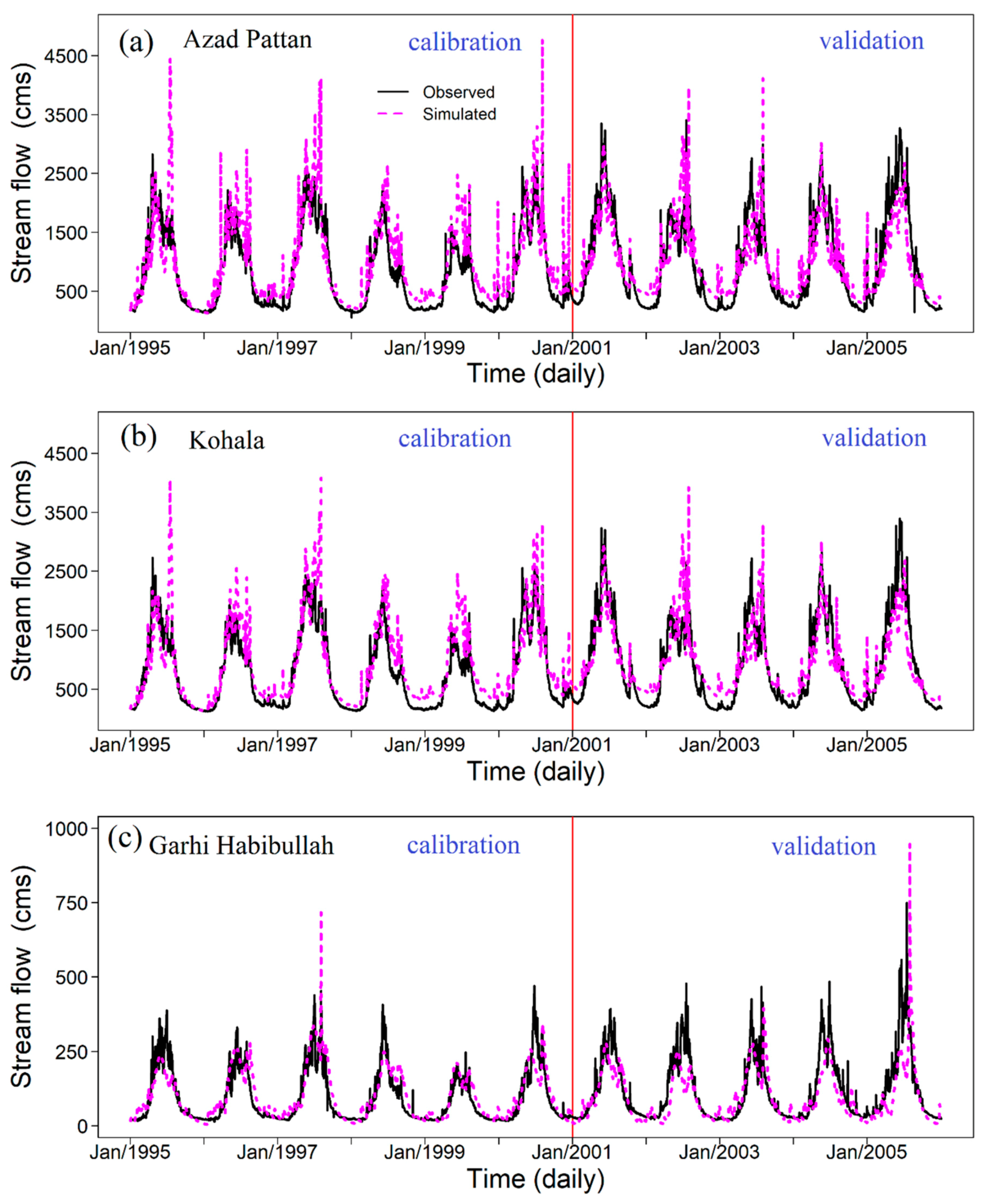
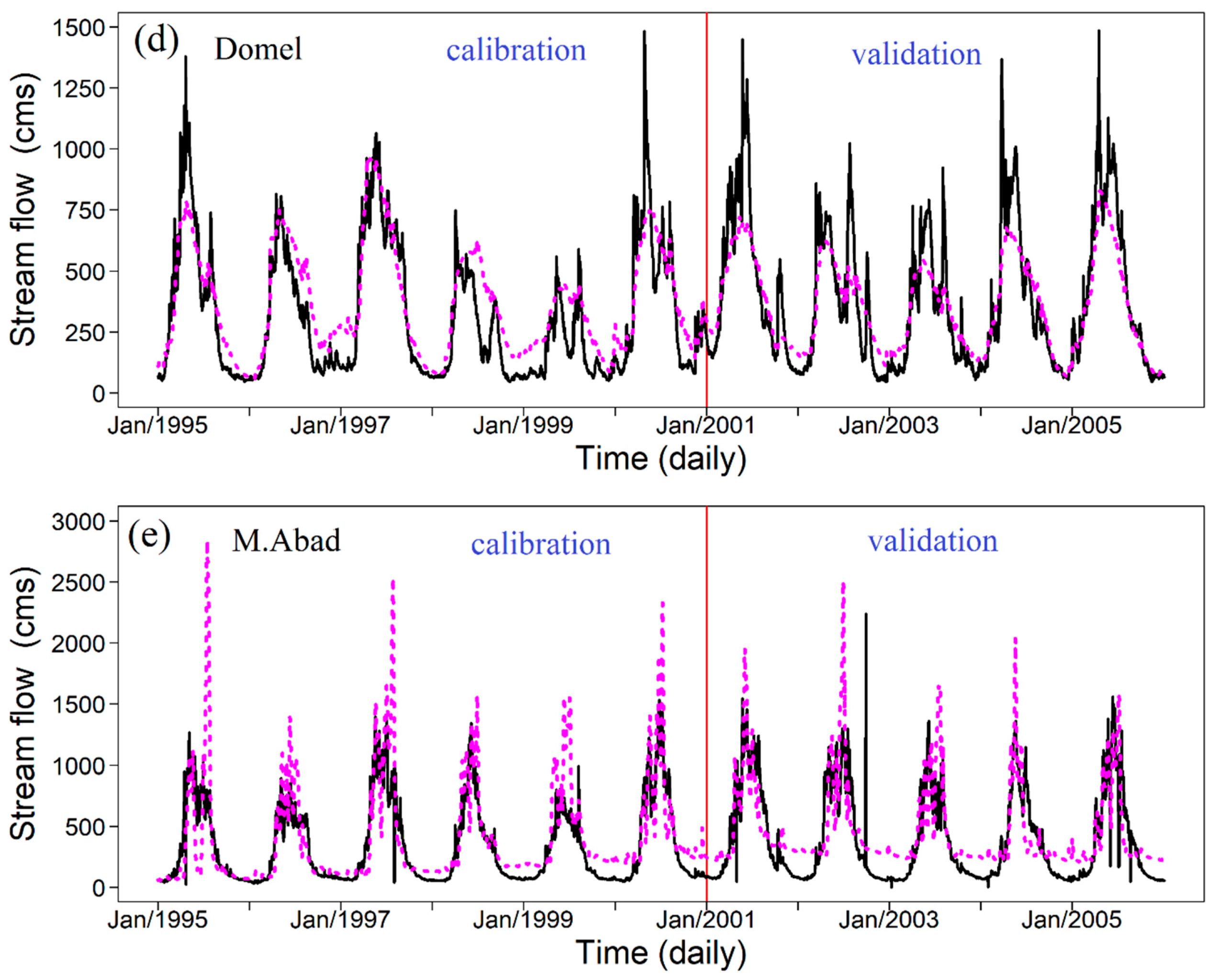
Figure 4 presents the results of daily streamflow during the calibration and validation of SWAT. Calibration was performed for the period from 1995–2001, and validation was conducted from 2002 to 2005. The calibrated parameters were used in the validation to simulate the discharge. The value of evaluation parameters, such as R2, NSE, PBIAS, and RSR, are shown in Table 5. At the daily time scale, the values of NSE and R2 were ranged from 0.56 to 0.81 and 0.52 to 0.81 during calibration and validation. At all the gauging stations except Kotli, the value of NSE was greater than 0.65 at a monthly scale. At different hydrological stations, trends of observed flows were well modeled. However, there are also very small over-estimations and under-estimations. Based on the performance classification of Moriasi et al., the results of model simulation fall under a good category [33]. Garee et al. also reported similar results over the Upper Indus Basin (UIB) using the SWAT model [36]. The topography, soil, and land-use were kept constant throughout the simulation period, which has a significant effect on streamflow [37]. Simulating streamflow should be based on good data collection via meteorology, hydrology, multi-period soil data, and land-use.
5.3. Future Temperature and Precipitation
The analysis of statistical models outputs showed that Tmax and Tmin increased in the range of 0.4 °C to 4.18 °C and 0.3° C to 4.2 °C, respectively, relative to reference period for the two-climate change scenarios with three GCMs. A decrease in seasonal temperature values was estimated in the spring under RCP4.5. SDSM and LARS-WG projected that the warmest season at the end of this century would be autumn, with a rise of mean minimum temperature between 4.11 °C and 4.66 °C [24].
Islam et al. and Garee et al. projected an increase in temperature over the UIB using RCM (PRECIS) and GCMs (EC-EARTH, CCSM4, and ECHAM6) outputs under different scenarios [36,38]. Mahmood et al. also reported an increase in temperature about 2.6 °C at the end of this century over the Jhelum River Basin using the HADCM3 outputs [22]. Overall, the above studies suggest that the JRB would face more warming in the future but with small differences in seasonal trends.
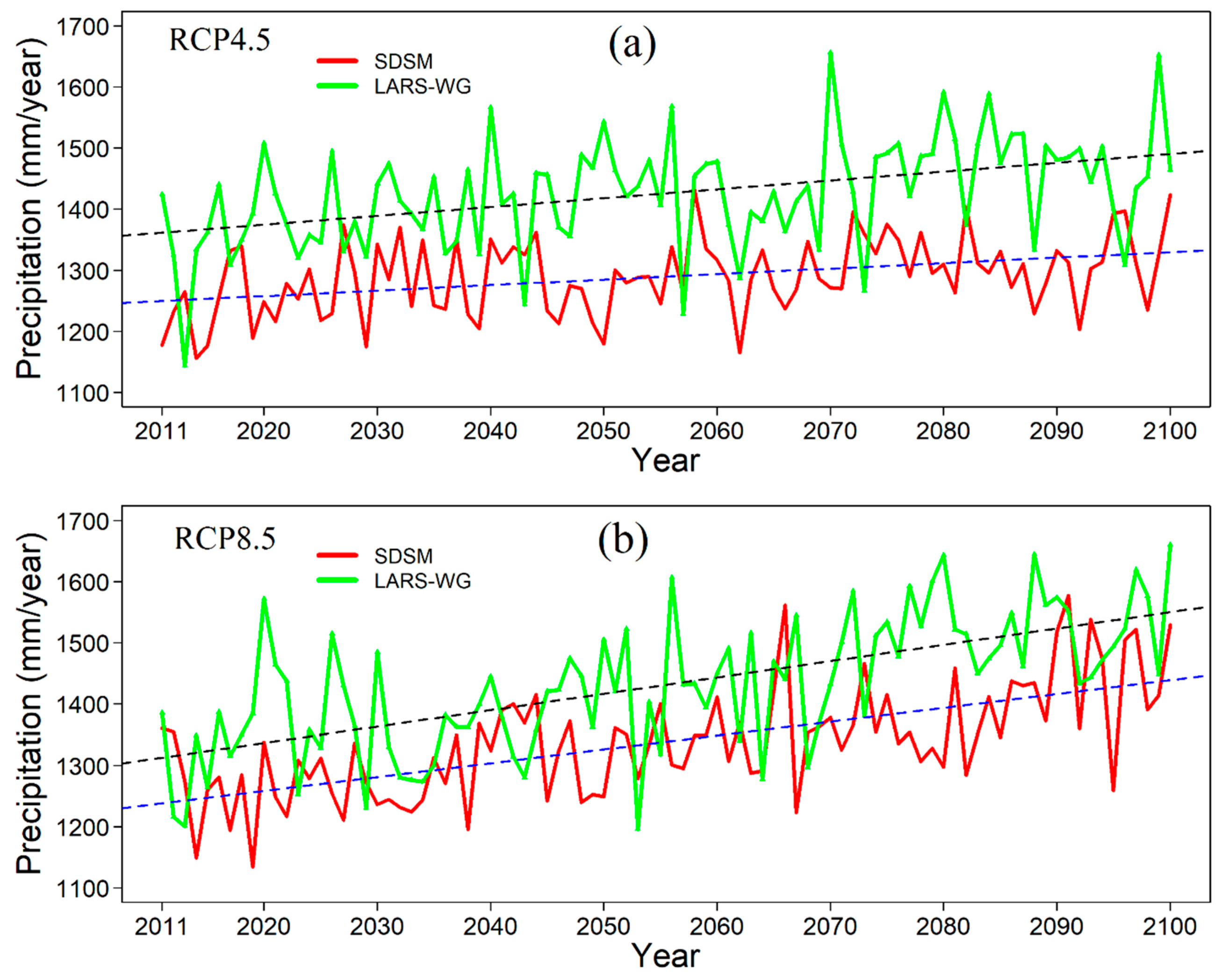
The precipitation projection using two RCPs scenarios for future periods is illustrated in Figure 5. A linear rising trend could be observed under both RCPs in JRB. The annual increment was higher under RCP8.5 as compared to RCP4.5. The modified Mann–Kendall test revealed that there was a significant positive trend in precipitation for RCP4.5 and RCP8.5 with p-values less than 0.01 at the 99% significance level. RCP 4.5 showed a positive slope (increasing) of 1 mm/year and 1.4 mm/year with SDSM and LARS-WG, while RCP 8.5 exhibited a slope of 2.1 mm/year and 2.8 mm/year with the Sen’s slope estimator.
Immerzeel et al. projected an increase in precipitation by 25% for 2046 to 2065 based on five GCMs over the Upper Indus Basin for the SRES A1B scenario [39]. Mahmood et al. also projected an increase in precipitation over the Jhelum River Basin by 12% and 14% towards the end of this century for A2 and B2 scenarios [40]. Similarly, projected annual precipitation increase over JRB was reported by [41] to be 45.52 mm in the 2080s compared to baseline using five GCMs data.
The future projection of precipitation mainly depends on the GCMs outputs. All the above-cited studies predict an increase in precipitation over the study area, while the used methodology and details differ.
5.4. Precipitation, Temperature, and CO2 Sensitivity Scenarios
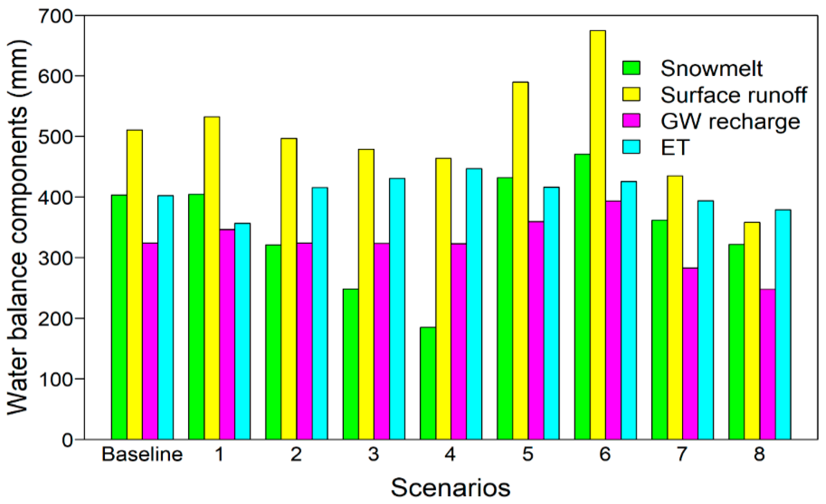
Figure 6 shows the average annual water balance components of JRB under different climatic scenarios, and Table 6 describes the hypothetical climate scenarios used in this study. It was seen that the surface runoff, ET, snowmelt, and groundwater (GW) recharge would be affected to a varying degree by the changes in precipitation or temperature in the future. The doubling of CO2 concentration (scenario-1) without any changes in precipitation and temperature could be observed; also, ET declined by 11.29%, and surface runoff increased by about 4.37%. Increased CO2 concentration has substantial impacts on plant physiology [42] through the reduced opening of the plant stomata, known as physiological forcing [43]. Physiological forcing can reduce ET, and reduced ET leaves more water in the soil profile, increasing the soil water content [44,45,46]. Moist soils can raise the water yield by generating more surface runoff, lateral flow, and seepage, all of which contribute to increasing streamflow [47,48]. Temperature rise (scenarios 2 to 4) caused a substantial decrease of snowmelt, surface runoff, and groundwater recharge. The average annual snowmelt (as snowfall decrease) was predicted to decrease by more than 50% in response to an increase in temperature by about 6 °C. Predicted ET showed an increase of 7.2% and 11.11% in response to 4 °C and 6 °C increase in temperature, respectively. However, under Scenarios 5 to 6 (increasing precipitation), the annual average surface runoff of basin would increase as well as the annual mean GW recharge. A large amount of precipitation is the major cause of an increase in runoff [28]. Huang and Zhang found that the main factor affecting surface runoff is precipitation and that any (positive or negative) trend in precipitation would affect runoff trends [49].
5.5. Impact of Future Climate Change on Streamflow
Future hydrological projections were divided into three periods (2020s, 2050s, and 2080s) for the assessment of the impact of climate change on the discharge of JRB (at Azad Pattan station), which were compared with the reference observed discharge (1976–2005).
5.5.1. Changes in Annual Flow
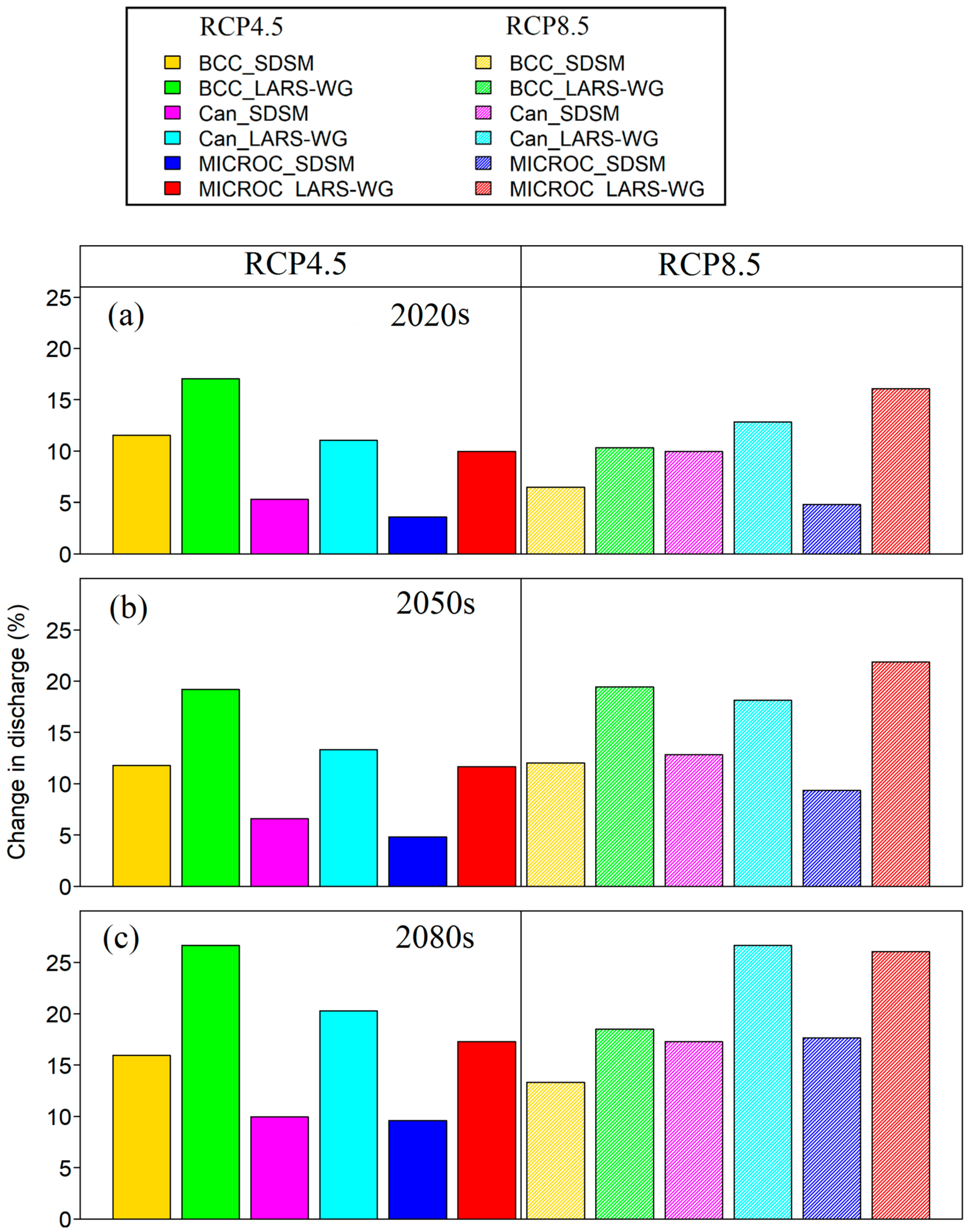
The changes in annual mean discharge under different climate change scenarios are shown in Figure 7. Focusing on the two downscaling techniques (SDSM and LARS-WG), the annual change in discharge (increase) derived from LARS-WG was higher in magnitude than SDSM under all the three future periods. Under RCP4.5, changes in projected annual discharge varied from 3.60% to 15.96% and 5.28% to 26.65% with SDSM and LARS-WG, respectively. Under RCP8.5, changes in projected annual discharge varied from 6.48% to 17.28% and 4.80% to 28.78% with SDSM and LARS-WG, respectively. In the 2080s, the maximum change in projected discharge was expected by using BCC-CSM1-1 under RCP4.5, and under RCP8.5 by using CanESM2.
Similar results were also found by [22], who assessed the impact of climate change in the Jhelum River Basin using the HADCM3 global climate model with SRES A2 and B2. The outcomes of the current study were also comparable with other regional and local climate change impact studies [36,39]. Most of the global climate model suggested that the annual streamflow would increase from 7.57% to 32.12% at the end of the 21st century.
This increase in streamflow may have positive and negative effects on water management and planning. Irrigation water for the Indus Basin Irrigation Systems (IBIS), which is the largest irrigation network in the world, is controlled through two major storage reservoirs (Jhelum River has a Mangla reservoir, and Indus River has Tarbela reservoir). Any change in the upstream water supply to these reservoirs will have a significant influence on thousands of farmers downstream. Our results indicated a substantial increase in future streamflow. Dependency on groundwater would also reduce in the future due to the availability of more surface water for irrigated agriculture and food security.
Mangla hydropower plant has a total installed capacity of 1000 MW, which is 15% of total electricity production through hydropower plants. The increase in projected streamflow can be used for electricity production. All the hydroelectric plants under construction are based on the Runoff River (ROR) design. The amount of electricity generated from ROR design depends on the daily flow. As the future streamflow is projected to increase, this type of hydroelectric plant can immensely benefit from climate change. A study conducted by [50] at Mangla hydropower plant showed that high streamflow is expected, which would result in an annual increase of 18.9% and 19.9% in electricity production under SRES A2 and B2 at the end of this century. The high electricity generation contribution is due to the increase in streamflow in winter.
5.5.2. Changes in Seasonal Flow
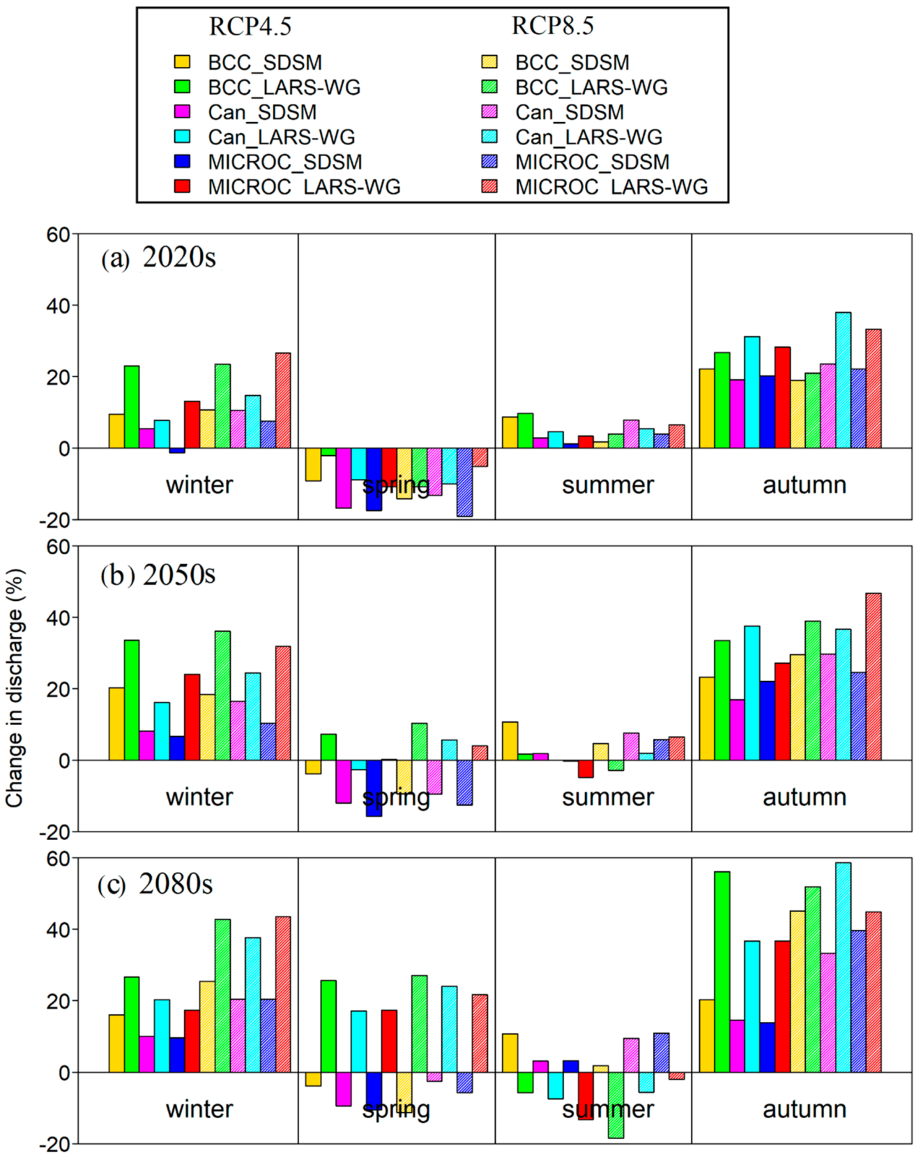
Figure 8 shows the changes in seasonal mean discharge under two scenarios using SDSM and LARS-WG for the three future time horizons. In winter and autumn, an increasing trend in streamflow was observed at Azad Pattan with both downscaling methods under RCP4.5 and RCP 8.5 in all the three periods. All the GCMs showed similar patterns (increasing) but different magnitudes. The LARS-WG simulated considerably higher discharge than SDSM in both seasons. In winter, the maximum increase of 26.56%, 31.89%, and 43.50% was calculated in the 2020s, 2050s, and 2080s, respectively, under RCP8.5. CanESM2 showed a maximum increase of 58.56% in autumn at Azad Pattan. In other seasons (spring and summer), the greatest differences in projected discharge could be observed between SDSM and LARS-WG. In the 2020s, the projected runoff would increase in winter, summer, and autumn, while would decrease in spring with both downscaling methods. SDSM and LARS-WG would behave differently in summer and spring in the 2080s. It can be seen by the passage of time that the discharge would significantly increase in spring and decrease in summer with LARS-WG. Under RCP8.5, changes in average seasonal flow were higher in magnitudes than RCP4.5 in three future time horizons.
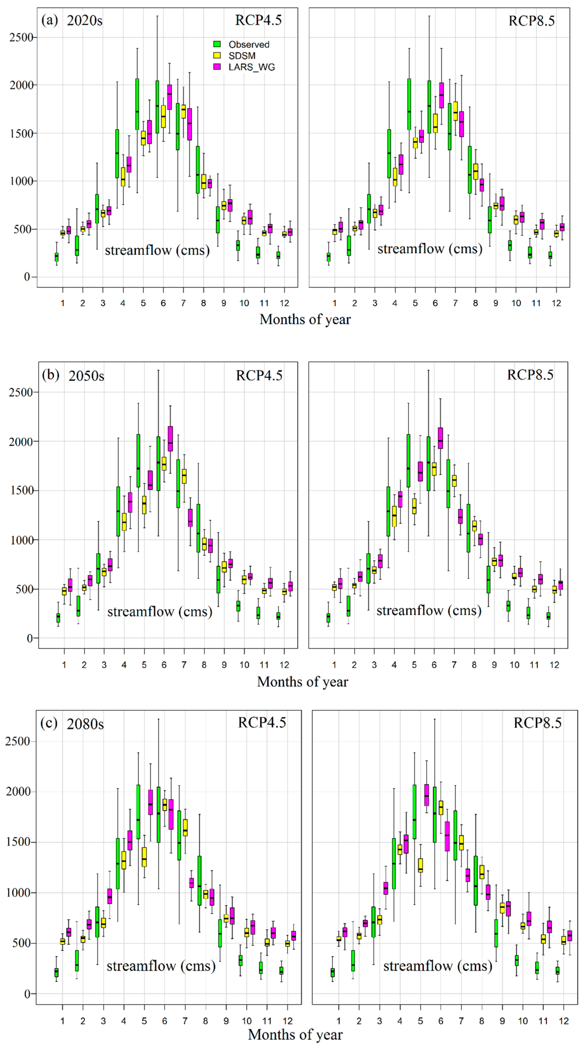
5.5.3. Changes in Monthly Flow
The impact of climate change on the monthly streamflow of the Jhelum River Basin is shown in Figure 9. The results showed that both of the downscaling methods predicted an increase in streamflow during the majority of months of the year.
Streamflow variability was higher in May, June, and July; corresponding months of the year had higher discharge. Peak streamflow was found in June in the 2020s and 2050s with both downscaling methods, but this peak was found to shift in May (2080s) using LARS-WG climatic data. LARS-WG showed higher discharge variability as compared to SDSM in all the future time slices (2020s, 2050s, and 2080s). In the 2020s, predicted streamflow was less than observed flow in March, April, and May with all scenarios using SDSM, but at the end of the century (2080s), predicted flow was higher as compared to observed during these months. The highest increase in the flow would be expected in low flow months (October, November, December, January, and February) with both RCP scenarios and downscaling methods.
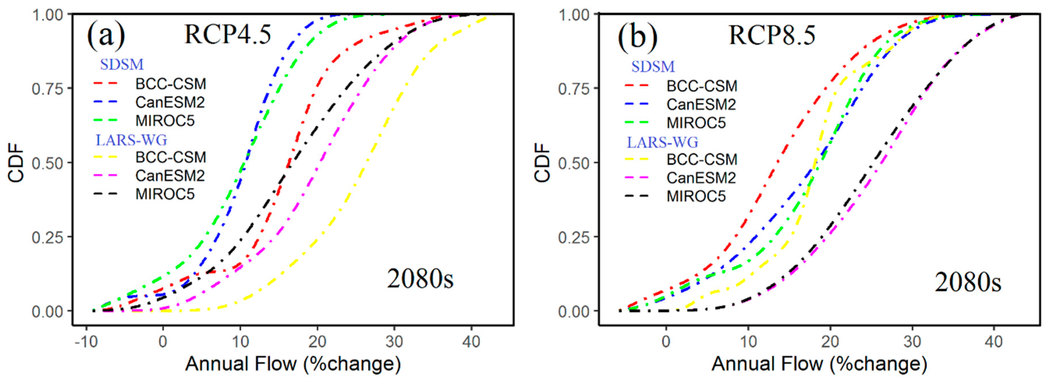
5.6. Uncertainty of Annual Flow Simulations
Figure 10 presents the Cumulative Distribution Function (CDFs) of annual discharge with two RCPs scenarios, two downscaling methods, and three GCMs (i.e., BCC-CSM, CanESM2, and MIROC5) for the Jhelum River Basin. Uncertainties of future streamflow projections were associated with each potential uncertainty element (downscaling method, GCM, and RCP). Overall, the flow was increasing during 2071–2100 with both downscaling methods using RCP4.5 and RCP8.5. The uncertainty associated with downscaling methods (SDSM and LARS-WG) was more as compared to uncertainty within GCMs in quantifying the impact of climate change on streamflow. Under RCP8.5, SDSM showed very less uncertainty in the flow values, especially at low and high ends. LARS-WG predicted a larger change in annual flow than the SDSM. Figure A1 and Figure A2 also present similar types of uncertainties during the 2020s and 2050s with both downscaling methods for RCP4.5 and RCP8.5. However, magnitudes of annual flow changes were relatively lower as compared to the 2080s.
5.7. Effects of Climate Change on Water Balance Components
Water balance components contribute to the river discharge and overall hydrological cycle of the basin (Bajracharya et al. 2018) [7]. Table 7 shows the mean annual values of all water balance components with SDSM and LARS-WG under both RCPs scenarios. However, surface runoff (SURQ) and groundwater flow (GWQ) demonstrated the highest increment. Surface runoff increased from 3.7% to 25.6% under RCP4.5 and 4.3% to 29.2% under RCP8.5. Likewise, ET and Potential Evapotranspiration (PET) showed the increment in all the scenarios. PET showed an increase ranging between 4.6% and 8.1%, 5.7% and 11%, and 6% and 16.6%, respectively, for the three future time horizons (2020s, 2050s, and 2080s). The increase of PET might lead to decrease moisture of soil and increase the plants’ water stress. This might reduce agriculture productivity, vegetation cover destruction, and the intensification of desertification in the basin during the 21st century.
Water yield is the net amount of water contributed by sub-basins and HRUs to the streamflow [7]. It is the combination of surface runoff, lateral flow, and groundwater flow with any deduction in transmission losses and pond abstraction [51]. However, SDSM showed an increase in water yield of about 6.8% to 16% under both scenarios, while LARS-WG represented about 12.6% to 23.7%.
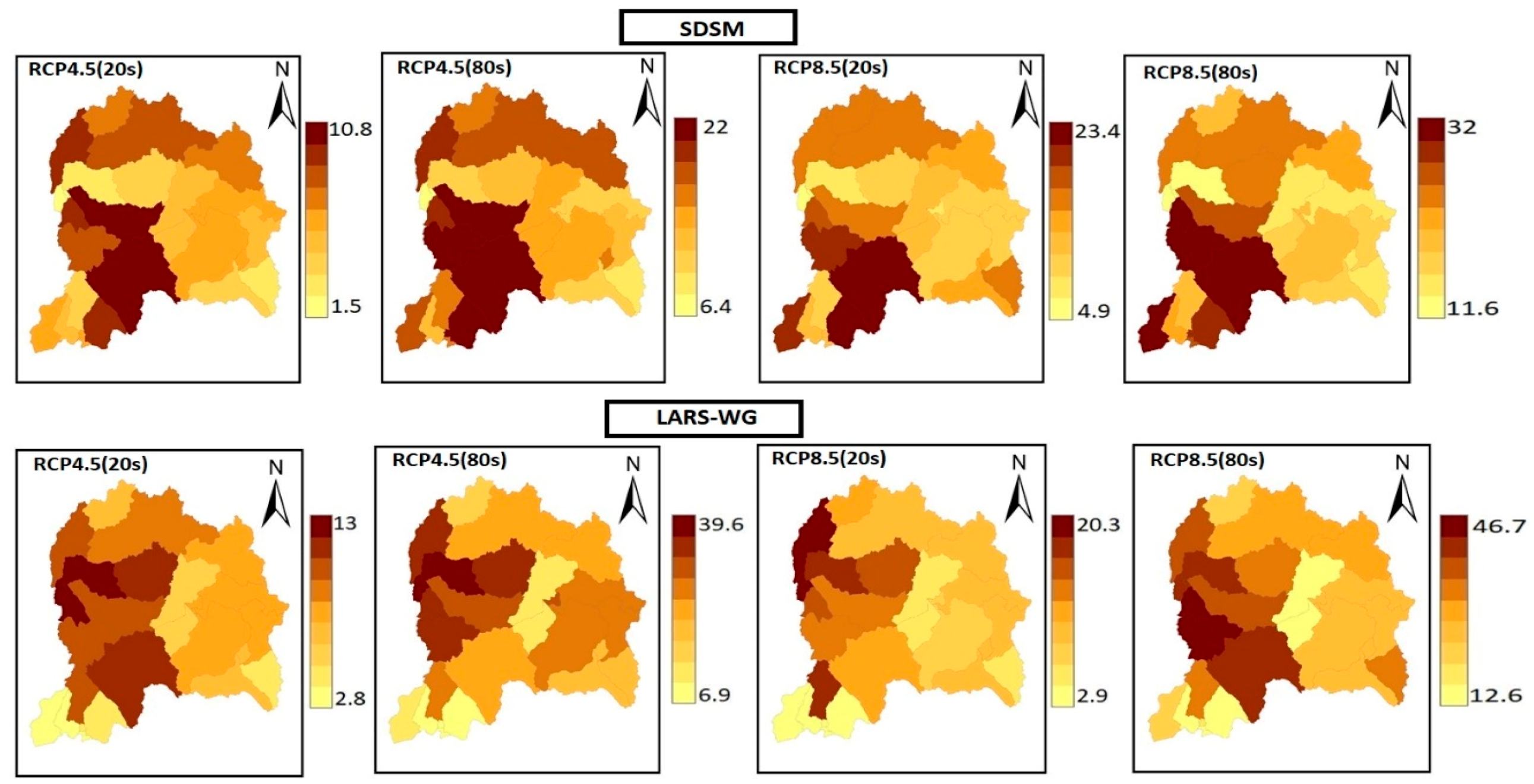
5.7.1. Impact on Water Yield
Figure 11 shows the spatial distribution patterns of percentage changes in mean annual water yield projected for different sub-basins in the 2020s and 2080s under RCP4.5 and RCP8.5, using climatic data of SDSM and LARS-WG relative to the baseline. All the sub-basins showed an increase in water yield, and the changes ranged between 1.5% to 46.7% over the whole basin. RCP4.5 and RCP8.5 had similar spatial patterns of water yield changes for the two future periods; however, RCP8.5 showed a higher increase as compared to RCP4.5 with both downscaling methods. As can be seen that while the water yield projected by using the SDSM-downscaled data was more significant in the southwest part of the basin (except two sub-basins), this pattern was more pronounced in the western part (except lower sub-basins) of a watershed using LARS-WG-downscaled data. It can also be observed that the sub-basins located in the eastern part of the watershed showed less increase in water yield as these sub-basins receive snowfall, which would decrease with a rise in temperature in the future.
5.7.2. Impact on Evapotranspiration (Green Water Flow)
Figure 12 presents the changes in the spatial distribution of average annual actual evapotranspiration (ET) as compared to baseline under RCP scenarios (RCP4.5 and RCP8.5) with SDSM and LARS-WG in three future time horizons. Due to the increase in precipitation and temperature in the future, the ET of the basin would be affected significantly. This increase in temperature would cause the ET to rise as well. By using projected climatic data of SDSM, the mean annual ET changes ranged from 2.1% to 23.1% under RCP4.5, whereas under RCP8.5, these changes ranged from 4.9% to 32% during the two future periods. The mean annual ET changes (positive) projected by using LARS-WG data could reach as much as 43.2% under RCP8.5 in the 2080s. These results are also consistent with prior studies in South Asia [7,52].
In the case of SDSM, green water flow was more pronounced in the eastern part and southwest lower sub-basins, while for LARS-WG, these changes were more significant only in the eastern part under RCP4.5 and RCP8.5. This increase in green water flow was more substantial in the sub-basin at high elevation (basin cover with snow) as projected temperature increase caused a shortening of snow cover season.
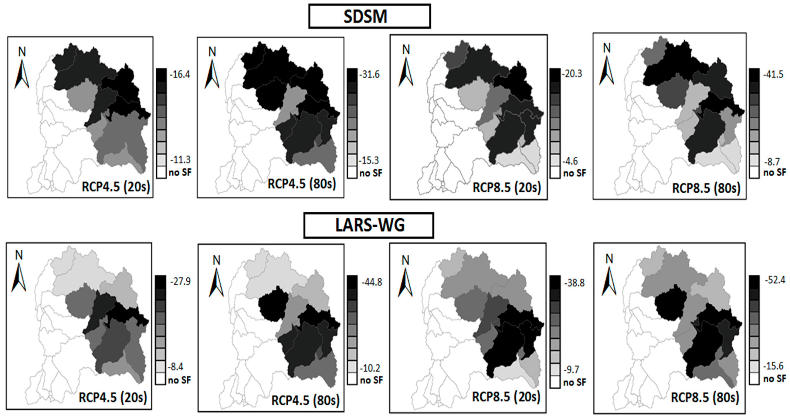
5.7.3. Impact on Snowmelt
Figure 13 illustrates the spatial distribution in percentage changes of snowmelt during the 2020s and 2080s compared to the reference period in different sub-basins of the Jhelum River Basin using SDSM and LARS-WG under RCP4.5 and RCP8.5. The sub-basins located at lower elevation have relatively higher temperatures due to which no snowfall is observed. The decrease in snowmelt would be progressive in the future period as the basin would face more warming. Under RCP4.5, a moderate decrease (ranging from −11.3% to −16.4%) in snowmelt with SDSM was observed during the 2020s. The maximum decrease in snowmelt was projected during the 2080s with LARS-WG up to −52.4% under RCP8.5. Both RCPs scenarios projected a decrease in snowmelt, but this reduction was relatively higher under RCP8.5.
It can be seen that the western part of the basin was not affected by changes in snowmelt, as these sub-basins are snow-free throughout the year. The sub-basin in the eastern part of the watershed showed a significant decrease in snowmelt with both downscaling methods. Using the climatic data of SDSM, the decrease was more pronounced in the northeast part of the basin.
6. Conclusions
In this study, to investigate the impacts of projected climate change (2011–2100) on the hydrological regimes of Jhelum River Basin, 12 climate projections combining three GCMs (i.e., BCC-CSM1.1, CanESM2, and MIROC5), two statistical downscaling methods (SDSM and LARS-WG), and two RCPs emission scenarios (RCP4.5 and RCP8.5) were considered. The Soil and Water Assessment Tool (SWAT) was used for the simulation of hydrological regimes in JRB. The SWAT model was calibrated and validated using the snow parameters at the sub-basin scale. The SWAT model simulated discharge was compared with observed discharge at the five different hydrological stations that lie at various geographical locations, for both calibration (1995–2001) and validation (2002–2005) periods. The NSE and R2 values (>0.65 at most stations) showed the model’s ability to reproduce streamflow, with reasonable accuracy. The calibrated model was employed to study the influence of projected climate on water resources. Under the IPCC RCP8.5 (high emissions) scenario, the annual mean temperature of the basin expected to increase by 1.8 °C and 3.7 °C with SDSM and LARS-WG, respectively. Similarly, the projected annual mean precipitation would increase by 15.4% and 28.3% during the late century (2071–2100) under RCP8.5.
The results of climate sensitivity studies revealed that the hydrology of JRB is highly sensitive to climate change scenarios. Out of all scenarios, scenario 6 (precipitation increase 20%) represented a maximum increase in annual mean surface runoff, snowmelt, groundwater recharge, and ET from the baseline condition, whereas the scenario 7 (precipitation decrease 20%) showed a maximum decrease in all water balance components. The average annual snowmelt (as snowfall decrease) was predicted to decrease by more than 50% in response to an increase in temperature by about 6 °C.
The mean annual streamflow was projected to rise under RCP4.5 and RCP8.5 using the three GCMs with SDSM and LARS-WG. However, the prediction was different for all the 12 scenarios (downscaling methods, GCMs, and RCPs). CanESM2 predicted the highest increase in streamflow by about 28.78% under RCP8.5 with LARS-WG. Substantial variations in seasonal streamflow would be observed when compared with the baseline period (1976–2005). Winter and autumn showed an increase in predicted flow under all the scenarios in three future horizons (2020s, 2050s, and 2080s). The seasons with most inconsistent results, and so, the ones for which to draw clear conclusions was challenging, were summer and spring, for which either future streamflow could increase or decrease based on the projected climatic data (downscaling method). On a monthly scale, in the 2030s, the predicted streamflow would increase in all months except March, April, and May. According to LARS-WG, peak discharge would shift from June to May under both RCP scenarios.
Climate change also has a significant effect on the spatial and temporal variation of water balance components in the Jhelum River Basin. The ensemble means of three GCMs exhibited an increase in mean annual surface runoff, groundwater recharge, lateral flow, ET, and water yield with SDSM and LARS-WG for RCP4.5 and RCP8.5. The spatial distribution of projected water yield showed an increase in all sub-basins of the watershed. However, this increase was more pronounced in the western part of the basin as these sub-basins are mostly dependent on rainfall (no snowfall). On the other hand, green water flow (ET) under RCP8.5 was more pronounced in the sub-basin at high elevation (basin cover with snow-eastern part) as projected temperature increase caused a shortening of snow cover season. Spatial distribution of snowmelt revealed that, in the future, snowmelt (as snowfall decrease) could be decreased in the eastern part of the basin due to the rise of temperature. In general, climate change is expected to affect more sub-basins at high-altitude.
Different uncertainties sources (GCMs, downscaling techniques, and RCPs) were involved in the impact studies. The results showed that the uncertainty associated with downscaling methods (SDSM and LARS-WG) was higher than GCMs itself. Some conclusions can be drawn from the hydrological modeling results, even if the uncertainty quantification was not part of the present study. Under RCP8.5, SDSM showed very less uncertainty in the flow values, especially at low and high ends. LARS-WG predicted larger changes in annual flow than the SDSM.
Our research outcomes would be helpful for the effective planning and management of water demand and supply in the Jhelum River Basin to consider the impact of climate change. The hydropower plant in operation and several potential hydropower projects would benefit from considering future changes in the regional hydrological cycle. More specifically, they could help to comprehend better the future hydro-climatic variability, which is vital to design the hydroelectric power plants. In general, the positive effect of climate change could be the availability of sufficient water from the catchment, but sometimes, a high amount of water leads to flooding.
Author Contributions
Conceptualization, N.S. and C.B.; Methodology, N.S.; Model calibration and validation, N.S.; Formal Analysis, M.U.; Data curation, N.S.; Writing—Original Draft Preparation, N.S. and M.U.; Writing—Review and Editing, N.S. and C.B.; Supervision, C.B.
Funding
This research received no external funding.
Acknowledgments
The first author was financially supported by the doctoral scholarship from the Higher Education Commission of Pakistan (HEC), Pakistan, and German Academic Exchange Service (DAAD), Germany. The authors wish to acknowledge the Water and Power Development Authority (WAPDA), Pakistan Meteorological Department (PMD), and Indian Meteorological Department (IMD) for providing data used in this study. We extend our thanks to the Institute of Hydrology and Meteorology, Chair of Meteorology, Technische Universität Dresden for giving the opportunity to perform this research. Open Access Funding by the Publication Fund of the TU Dresden.
Conflicts of Interest
The authors declare no conflict of interest.
Appendix A

Table A1.
Climate models used to project climate change scenarios.
| GCM | Development Countries | Spatial Resolution (°) | Time Span | ||
|---|---|---|---|---|---|
| Longitude | Latitude | Historical | Future (RCPs) | ||
| BCC-CSM1-1 | China | 2.812 | 2.812 | 1950–2005 | 2006–2100 |
| MIROC5 | Japan | 2.812 | 2.812 | 1950–2005 | 2006–2100 |
| CanESM2 | Canada | 1.406 | 1.406 | 1950–2005 | 2006–2100 |
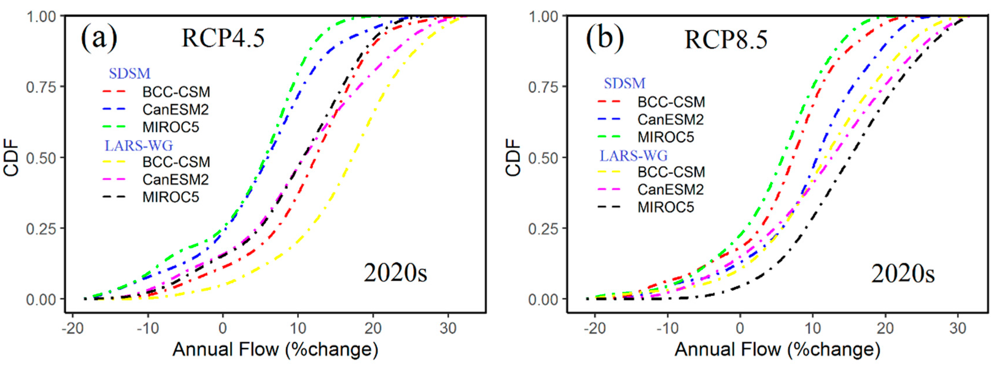
Figure A1.
CDFs of annual changes in flow under (a) RCP4.5 and (b) RCP8.5 between the period 2011–2040 and 1975–2005, reflecting the uncertainty of SDSM and LARS-WG.
Figure A1.
CDFs of annual changes in flow under (a) RCP4.5 and (b) RCP8.5 between the period 2011–2040 and 1975–2005, reflecting the uncertainty of SDSM and LARS-WG.

Table A2.
Model performance rating based on Moriasi et al. [33].
Table A2.
Model performance rating based on Moriasi et al. [33].
| NSE | RSR | PBIAS | Performance Rating |
|---|---|---|---|
| 0.75–1 | 0–0.5 | <±10 | Very good |
| 0.65–0.75 | 0.5–0.6 | ±10 to ±15 | Good |
| 0.5–0.65 | 0.6–0.7 | ±15 to ± 25 | Satisfactory |
| <0.5 | >0.7 | >±25 | Unsatisfactory |
Figure A2.
CDFs of annual changes in flow under (a) RCP4.5 and (b) RCP8.5 between the period 2041–2070 and 1975–2005, reflecting the uncertainty of SDSM and LARS-WG.
Figure A2.
CDFs of annual changes in flow under (a) RCP4.5 and (b) RCP8.5 between the period 2041–2070 and 1975–2005, reflecting the uncertainty of SDSM and LARS-WG.

References
- IPCC. Climate Change 2013: The Physical Science Basis; Contribution of Working Group I to the Fifth Assessment Report of the Intergovernmental Panel on Climate Change. Intergovernmental Panel on Climate Change, Working Group I Contribution to the IPCC Fifth Assessment Report (AR5); Cambridge University Press: New York, NY, USA, 2013; p. 1535. [Google Scholar] [CrossRef]
- Singh, D.; Jain, S.K.; Gupta, R.D. Trend in observed and projected maximum and minimum temperature over N-W Himalayan basin. J. Mt. Sci. 2015, 12, 417–433. [Google Scholar] [CrossRef]
- Ahmad, S. Change in glaciers length in the Indian Himalaya: an observation and prediction under warming scenario. Model. Earth Syst. Environ. 2016, 2, 1–10. [Google Scholar] [CrossRef] [Green Version]
- Dahal, N.; Shrestha, U.; Tuitui, A.; Ojha, H. Temporal Changes in Precipitation and Temperature and their Implications on the Streamflow of Rosi River. Cent. Nepal Clim. 2018, 7, 3. [Google Scholar] [CrossRef]
- Immerzeel, W.W.; van Beek, L.P.H.; Konz, M.; Shrestha, A.B.; Bierkens, M.F.P. Hydrological response to climate change in a glacierized catchment in the Himalayas. Clim. Chang. 2012, 110, 721–736. [Google Scholar] [CrossRef] [PubMed]
- Gosling, S.N.; Taylor, R.G.; Arnell, N.W.; Todd, M.C. A comparative analysis of projected impacts of climate change on river runoff from global and catchment-scale hydrological models. Hydrol. Earth Syst. Sci. 2011, 15, 279–294. [Google Scholar] [CrossRef] [Green Version]
- Bajracharya, A.R.; Bajracharya, S.R.; Shrestha, A.B.; Maharjan, S.B. Climate change impact assessment on the hydrological regime of the Kaligandaki Basin, Nepal. Sci. Total Environ. 2018, 625, 837–848. [Google Scholar] [CrossRef]
- Tan, M.L.; Ibrahim, A.L.; Yusop, Z.; Chua, V.P.; Chan, N.W. Climate change impacts under CMIP5 RCP scenarios on water resources of the Kelantan River Basin, Malaysia. Atmos. Res. 2017, 189, 1–10. [Google Scholar] [CrossRef]
- Sellami, H.; Benabdallah, S.; La Jeunesse, I.; Vanclooster, M. Climate models and hydrological parameter uncertainties in climate change impacts on monthly runoff and daily flow duration curve of a Mediterranean catchment. Hydrol. Sci. J. 2016, 61, 1415–1429. [Google Scholar] [CrossRef]
- Zhang, Y.; You, Q.; Chen, C.; Ge, J. Impacts of climate change on streamflows under RCP scenarios: A case study in Xin River Basin, China. Atmos. Res. 2016, 178–179, 521–534. [Google Scholar] [CrossRef]
- Mishra, Y.; Nakamura, T.; Babel, M.S.; Ninsawat, S.; Ochi, S. Impact of climate change on water resources of the Bheri River Basin, Nepal. Water 2018, 10, 220. [Google Scholar] [CrossRef]
- Chen, J.; Brissette, F.P.; Leconte, R. Uncertainty of downscaling method in quantifying the impact of climate change on hydrology. J. Hydrol. 2011, 401, 190–202. [Google Scholar] [CrossRef]
- Wilby, R.L.; Harris, I. A framework for assessing uncertainties in climate change impacts: Low-flow scenarios for the River Thames, UK. Water Resour. Res. 2006, 42, 1–10. [Google Scholar] [CrossRef]
- Meaurio, M.; Zabaleta, A.; Boithias, L.; Epelde, A.M.; Sauvage, S.; Sánchez-Pérez, J.M.; Antiguedad, I. Assessing the hydrological response from an ensemble of CMIP5 climate projections in the transition zone of the Atlantic region (Bay of Biscay). J. Hydrol. 2017, 548, 46–62. [Google Scholar] [CrossRef]
- Teutschbein, C.; Wetterhall, F.; Seibert, J. Evaluation of different downscaling techniques for hydrological climate-change impact studies at the catchment scale. Clim. Dyn. 2011, 37, 2087–2105. [Google Scholar] [CrossRef]
- Chen, W.; Chau, K.W. Intelligent manipulation and calibration of parameters for hydrological models. Int. J. Environ. Pollut. 2006, 28, 432. [Google Scholar] [CrossRef]
- Martinec, J.; Rango, A.; Roberts, R. Snowmelt Runoff Model (SRM) User’s Manual; Agricultural Experiment Station Special Report 100; College of Agriculture and Home Economics: Las Cruces, NM, USA, 2008; p. 180. [Google Scholar] [CrossRef]
- Neitsch, S.L.; Arnold, J.G.; Kiniry, J.R.; Williams, J.R. Theoretical Documentation SWAT; Texas Water Resources Institute: College Station, TX, USA, 2011. [Google Scholar]
- Perazzoli, M.; Pinheiro, A.; Kaufmann, V. Assessing the impact of climate change scenarios on water resources in southern Brazil. Hydrol. Sci. J. 2012, 58, 77–87. [Google Scholar] [CrossRef]
- Shi, P.; Ma, X.; Hou, Y.; Li, Q.; Zhang, Z.; Qu, S.; Fang, X. Effects of Land-Use and Climate Change on Hydrological Processes in the Upstream of Huai River, China. Water Resour. Manag. 2013, 27, 1263–1278. [Google Scholar] [CrossRef]
- Yin, J.; Yuan, Z.; Yan, D.; Yang, Z.; Wang, Y. Addressing climate change impacts on streamflow in the Jinsha River basin based on CMIP5 climate models. Water 2018, 10, 910. [Google Scholar] [CrossRef]
- Mahmood, R.; Jia, S. Assessment of impacts of climate change on the water resources of the transboundary Jhelum River Basin of Pakistan and India. Water 2016, 8, 246. [Google Scholar] [CrossRef]
- Archer, D.R.; Fowler, H.J. Using meteorological data to forecast seasonal runoff on the River Jhelum, Pakistan. J. Hydrol. 2008, 361, 10–23. [Google Scholar] [CrossRef]
- Saddique, N.; Bernhofer, C.; Kronenberg, R.; Usman, M. Downscaling of CMIP5 Models Output by Using Statistical Models in a Data Scarce Mountain Environment (Mangla Dam Watershed), Northern Pakistan. Asia-Pac. J. Atmos. Sci. 2019. [Google Scholar] [CrossRef]
- Agarwal, C.S.; Garg, P.K. Textbook on Remote Sensing: In Natural Resources Monitoring and Management; A H Wheeler Publishing Co. Ltd.: Allahabad, India, 2002. [Google Scholar]
- Singh, D.; Gupta, R.D.; Jain, S.K. Assessment of impact of climate change on water resources in a hilly river basin. Arab. J. Geosci. 2015, 8, 10625–10646. [Google Scholar] [CrossRef]
- Shrestha, M.S.; Artan, G.A.; Bajracharya, S.R.; Sharma, R.R. Using satellite-based rainfall estimates for streamflow modelling: Bagmati Basin. J. Flood Risk Manag. 2008, 1, 89–99. [Google Scholar] [CrossRef]
- Bekele, D.; Alamirew, T.; Kebede, A.; Zeleke, G.; MMelesse, A. Modeling Climate Change Impact on the Hydrology of Keleta Watershed in the Awash River Basin, Ethiopia. Environ. Model. Assess. 2019, 24, 95–107. [Google Scholar] [CrossRef]
- Babar, Z.A.; Zhi, X.F.; Fei, G. Precipitation assessment of Indian summer monsoon based on CMIP5 climate simulations. Arab. J. Geosci. 2015, 8, 4379–4392. [Google Scholar] [CrossRef]
- Li, R.; Lv, S.; Han, B.; Gao, Y.; Meng, X. Projections of South Asian summer monsoon precipitation based on 12 CMIP5 models. Int. J. Climatol. 2017, 37, 94–108. [Google Scholar] [CrossRef]
- Mahmood, R.; Jia, S. An extended linear scaling method for downscaling temperature and its implication in the Jhelum River basin, Pakistan, and India, using CMIP5 GCMs. Theor. Appl. Climatol. 2017, 130, 725–734. [Google Scholar] [CrossRef]
- Abbaspour, K.C. SWAT-CUP: SWAT Calibration and Uncertainty Programs—A User Manual, Department of Systems Analysis, Intergrated Assessment and Modelling (SIAM), EAWAG; User Manual; Swiss Federal Institute of Aquatic Science and Technology: Duebendorf, Switzerland, 2015; p. 100. [Google Scholar] [CrossRef]
- Moriasi, D.N.; Arnold, J.G.; Liew, M.W.V.; Bingner, R.L.; Harmel, R.D.; Veith, T.L. Model evaluation guidelines for systematic quantification of accuracy in watershed simulations. Trans. ASABE 2007, 50, 885–900. [Google Scholar] [CrossRef]
- Santhi, C.; Arnold, J.G.; Williams, J.R.; Dugas, W.A.; Srinivasan, R.; Hauck, L.M. Validation of the SWAT model on a large river basin with point and nonpoint sources. J. Am. Water Resour. Assoc. 2001, 37, 1169–1188. [Google Scholar] [CrossRef]
- Willmott, C.J.; Robeson, S.M.; Matsuura, K. Short Communication a refined index of model performance. Int. J. Climatol. 2012, 32, 2088–2094. [Google Scholar] [CrossRef]
- Garee, K.; Chen, X.; Bao, A.; Wang, Y.; Meng, F. Hydrological Modeling of the Upper Indus Basin: A Case Study from a High-Altitude Glacierized Catchment Hunza. Water 2017, 9, 17. [Google Scholar] [CrossRef]
- Jing, Z.; Dan, H.; Xie, Y.; Yong, L.; Yang, Y.; Hu, S.; Guo, H.; Lei, Z.; Rui, Z. Integrated SWAT model and statistical downscaling for estimating streamflow response to climate change in the Lake Dianchi watershed, China. Stoch. Environ. Res. Risk Assess. 2015, 29, 1193–1210. [Google Scholar]
- Islam, S.; Rehman, N.; Sheikh, M.; Khan, A. Assessment of Future Changes in Temperature Related Extreme Indices over Pakistan Using Regional Climate Model Precis; Research Report GCISC-RR-05; Global Change Impact Study Centre: Islamabad, Pakistan, 2009.
- Immerzeel, W.W.; Van Beek, L.P.; Bierkens, M.F. Climate change will affect the Asian water towers. Science 2010, 328, 1382–1385. [Google Scholar] [CrossRef] [PubMed]
- Mahmood, R.; Babel, M.S. Evaluation of SDSM developed by annual and monthly sub-models for downscaling temperature and precipitation in the Jhelum basin, Pakistan and India. Theor. Appl. Climatol. 2013, 113, 27–44. [Google Scholar] [CrossRef]
- Azmat, M.; Qamar, M.U.; Ahmed, S.; Shahid, M.A.; Hussain, E.; Ahmad, S.; Khushnood, R.A. Ensembling Downscaling Techniques and Multiple GCMs to Improve Climate Change Predictions in Cryosphere Scarcely Gauged Catchment. Water Resour. Manag. 2018, 32, 3155–3174. [Google Scholar] [CrossRef]
- Sellers, P.J.; Randall, D.A.; Collatz, G.J.; Berry, J.A.; Field, C.B.; Dazlich, D.A.; Zhang, C.; Collelo, G.D.; Bounoua, L. A revised land surface parameterization (SiB2) for atmospheric part1: model formulation. J. Clim. 1995, 9, 676–705. [Google Scholar] [CrossRef]
- Field, C.B.; Jackson, R.B.; Mooney, H.A. Stomatal responses to increased CO2: implications from the plant to the global scale. Plant Cell Environ. 1995, 18, 1214–1225. [Google Scholar] [CrossRef]
- Betts, A.K.; Chen, F.; Mitchell, K.E.; Janjić, Z. Assessment of the Land Surface and Boundary Layer Models in Two Operational Versions of the NCEP Eta Model Using FIFE Data. Mon. Weather Rev. 2002, 125, 2896–2916. [Google Scholar] [CrossRef]
- Hungate, B.A.; Reichstein, M.; Dijkstra, P.; Johnson, D.; Hymus, G.; Tenhunen, J.D.; Drake, B.G. Evapotranspiration and soil water content in a scrub-oak woodland under carbon dioxide enrichment. Glob. Chang. Biol. 2002, 8, 289–298. [Google Scholar] [CrossRef]
- Stockle, C.O.; Dyke, P.T.; Williams, J.R.; Jones, C.A.; Rosenberg, N.J. A method for estimating the direct and climatic effects of rising atmospheric carbon dioxide on growth and yield of crops: Part II-Sensitivity analysis at three sites in the Midwestern USA. Agric. Syst. 1992, 38, 239–256. [Google Scholar] [CrossRef]
- Ficklin, D.L.; Luo, Y.; Luedeling, E.; Zhang, M. Climate change sensitivity assessment of a highly agricultural watershed using SWAT. J. Hydrol. 2009, 374, 16–29. [Google Scholar] [CrossRef]
- Wu, Y.; Liu, S.; Abdul-Aziz, O.I. Hydrological effects of the increased CO 2 and climate change in the Upper Mississippi River Basin using a modified SWAT. Clim. Chang. 2012, 110, 977–1003. [Google Scholar] [CrossRef]
- Huang, M.; Zhang, L. Hydrological responses to conservation practices in a catchment of the Loess Plateau, China. Hydrol. Process. 2004, 18, 1885–1898. [Google Scholar] [CrossRef]
- Mahmood, R. Assessment of Climate Change Impact on Water Resources and Hydropower in the Jhelum River Basin, Pakistan. Ph.D. Thesis, Asian Institute of Technology, Khlong Nueng, Thailand, 2013. [Google Scholar]
- Arnold, J.G.; Srinivasan, R.; Muttiah, R.S.; Williams, J.R. Large area hydrologic modeling and assessment part I: model development. J. Am. Water Res. Assoc. 1998, 34, 73–89. [Google Scholar] [CrossRef]
- Bharati, L.; Gurung, P.; Jayakody, P.; Smakhtin, V.; Bhattarai, U. The Projected Impact of Climate Change on Water Availability and Development in the Koshi Basin, Nepal. Mt. Res. Dev. 2014, 34, 118–130. [Google Scholar] [CrossRef]
Figure 1.
Location map of Jhelum River Basin and spatial distribution of weather and hydrological stations.
Figure 1.
Location map of Jhelum River Basin and spatial distribution of weather and hydrological stations.

Figure 2.
(a) Land-use and (b) Soil map of the study area.

Figure 3.
Sub-basins generated during delineation.

Figure 4.
Comparison of the observed and simulated stream (m3/s) flow at different stations (a) Azad Pattan (b) Kohala (c) Garhi Habibullah (d) Domel (e) M. Abad for the calibration and validation in the Jhelum River Basin.
Figure 4.
Comparison of the observed and simulated stream (m3/s) flow at different stations (a) Azad Pattan (b) Kohala (c) Garhi Habibullah (d) Domel (e) M. Abad for the calibration and validation in the Jhelum River Basin.


Figure 5.
Total annual future precipitation trends using SDSM (Statistical Downscaling Model) and LARS-WG (Long Ashton Research Station Weather Generator) (a) RCP 4.5 and (b) RCP 8.5.
Figure 5.
Total annual future precipitation trends using SDSM (Statistical Downscaling Model) and LARS-WG (Long Ashton Research Station Weather Generator) (a) RCP 4.5 and (b) RCP 8.5.

Figure 6.
Values of water balance components (mm) under different climate change scenarios. GW, groundwater; ET, evapotranspiration.
Figure 6.
Values of water balance components (mm) under different climate change scenarios. GW, groundwater; ET, evapotranspiration.

Figure 7.
Annual runoff changes (%) relative to baseline simulations with SDSM and LARS-WG in three different time horizons (a) 2020s, (b) 2050s, and (c) 2080s and two RCPs.
Figure 7.
Annual runoff changes (%) relative to baseline simulations with SDSM and LARS-WG in three different time horizons (a) 2020s, (b) 2050s, and (c) 2080s and two RCPs.

Figure 8.
Changes in seasonal discharge (relative to baseline) with SDSM and LARS-WG in three future periods (a) 2020s, (b) 2050s, and (c) 2080s under RCP4.5 and RCP8.5.
Figure 8.
Changes in seasonal discharge (relative to baseline) with SDSM and LARS-WG in three future periods (a) 2020s, (b) 2050s, and (c) 2080s under RCP4.5 and RCP8.5.

Figure 9.
Boxplot of monthly streamflow (m3/s), comparison of observed with SDSM and LARS-WG, using RCP4.5 and RCP8.5 under three future periods (a) 2020s, (b) 2050s, and (c) 2080s.
Figure 9.
Boxplot of monthly streamflow (m3/s), comparison of observed with SDSM and LARS-WG, using RCP4.5 and RCP8.5 under three future periods (a) 2020s, (b) 2050s, and (c) 2080s.

Figure 10.
CDFs (Cumulative Distribution Function) of annual changes in flow under (a) RCP4.5, and (b) RCP8.5 between the period 2071–2100 and 1975–2005, reflecting the uncertainty of SDSM and LARS-WG.
Figure 10.
CDFs (Cumulative Distribution Function) of annual changes in flow under (a) RCP4.5, and (b) RCP8.5 between the period 2071–2100 and 1975–2005, reflecting the uncertainty of SDSM and LARS-WG.

Figure 11.
Spatial distribution of relative change rate (%) in water yield in the Jhelum River Basin with SDSM and LARS-WG under RCP4.5 and RCP8.5.
Figure 11.
Spatial distribution of relative change rate (%) in water yield in the Jhelum River Basin with SDSM and LARS-WG under RCP4.5 and RCP8.5.

Figure 12.
Spatial distribution of relative change rate (%) in actual evapotranspiration in the Jhelum River Basin with SDSM and LARS-WG under RCP4.5 and RCP8.5.
Figure 12.
Spatial distribution of relative change rate (%) in actual evapotranspiration in the Jhelum River Basin with SDSM and LARS-WG under RCP4.5 and RCP8.5.

Figure 13.
Spatial distribution of relative changes in snowmelt during the 2020s and 2080s over the JRB (Jhelum River Basin) under RCP4.5 and RCP8.5 using climatic data outputs of SDSM and LARS-WG; no SF—represents no snowfall.
Figure 13.
Spatial distribution of relative changes in snowmelt during the 2020s and 2080s over the JRB (Jhelum River Basin) under RCP4.5 and RCP8.5 using climatic data outputs of SDSM and LARS-WG; no SF—represents no snowfall.

Table 1.
Basic information about hydrological stations, discharge is for 1976–2005.
| Sr. No. | River | Station | Latitude (°N) | Longitude (°E) | Elevation (m) | Catchment Area (km2) | Discharge (m3/s) |
|---|---|---|---|---|---|---|---|
| F1 | Kunhar | Garhi Habibulllah | 34.40 | 73.38 | 810 | 2441 | 102 |
| F2 | Neelum | Muzaffarabad | 34.37 | 73.47 | 670 | 7420 | 327 |
| F3 | Jhelum | Domel | 34.36 | 73.47 | 695 | 14,390 | 335 |
| F4 | Jhelum | Kohala | 34.12 | 73.50 | 584 | 24,930 | 787 |
| F5 | Jhelum | Azad Pattan | 33.73 | 73.60 | 476 | 26,420 | 833 |
| F6 | Poonch | Kotli | 33.46 | 73.88 | 518 | 3742 | 133 |
| F7 | Kanshi | Palote | 33.22 | 73.43 | 400 | 869.7 | 6.5 |
Table 2.
Meteorological data (1961–2012) that were used in the SWAT (Soil and Water Assessment Tool) simulation.
Table 2.
Meteorological data (1961–2012) that were used in the SWAT (Soil and Water Assessment Tool) simulation.
| Sr. No. | Station Name | Longitude (°E) | Latitude (°N) | Elvevation (m, MSL) | Precipitation (mm/year) |
|---|---|---|---|---|---|
| 1 | Jhelum | 73.74 | 32.94 | 287 | 854 |
| 2 | Gujar khan | 73.13 | 33.25 | 458 | 830 |
| 3 | Kotli | 73.90 | 33.51 | 614 | 1245 |
| 4 | Plandri | 73.71 | 33.72 | 1401 | 1443 |
| 5 | Rawalkot | 73.76 | 33.86 | 1676 | 1397 |
| 6 | Murree | 73.38 | 33.91 | 2213 | 1779 |
| 7 | Bagh | 73.78 | 33.98 | 1067 | 1422 |
| 8 | Garidoptta | 73.62 | 34.22 | 814 | 1567 |
| 9 | Muzaffarabad | 73.47 | 34.37 | 702 | 1423 |
| 10 | Balakot | 73.35 | 34.55 | 995 | 1701 |
| 11 | Naran | 73.65 | 34.90 | 2362 | 1154 |
| 12 | Astore | 74.90 | 35.33 | 2168 | 534 |
| 13 | Kupwara | 74.25 | 34.51 | 1609 | 1245 |
| 14 | Gulmarg | 74.33 | 34.00 | 2705 | 1543 |
| 15 | Srinagar | 74.83 | 34.08 | 1587 | 721 |
| 16 | Qaziqund | 75.08 | 33.58 | 1690 | 1345 |
Table 3.
Land-use, soil, and slope report.
| Spatial Data | SWAT Class | Description | % Area | Area (km2) |
|---|---|---|---|---|
| Land-use | AGRL | Agriculture | 30.81 | 10,296.61 |
| FRST | Forest mixed | 27.88 | 9311.08 | |
| RNGE | Grass + sparse vegetation | 36.79 | 12,286.75 | |
| WATR | Water | 2.07 | 691.31 | |
| URMD | Residential-medium Density | 2.43 | 811.54 | |
| Soil | GLACIER-6998 | Gleysol | 0.39 | 130.24 |
| I-B-U-3712 | Gleyic Solonchaks | 48.52 | 16,166.51 | |
| Be78-2c-3679 | Luvic Chernozems | 0.69 | 232.42 | |
| Be72-3c-3672 | Calcaric Phaoeozems | 23.20 | 7765.82 | |
| Be73-2c-3673 | Calcic Chernozems | 1.03 | 344.48 | |
| Be79-2a-3680 | Mollic Planosols | 20.72 | 6933.33 | |
| WATER-6997 | Water | 0.19 | 65.09 | |
| I-X-c-3512 | Gelic Regosols | 1.08 | 363.10 | |
| Lo44-1b-3799 | Harplic Solonetz | 1.40 | 470.19 | |
| Be71-2-3a-3668 | Gleyic Solonetz | 1.11 | 370.75 | |
| Rc40-2b-3843 | Haplic Chernozems | 1.66 | 555.48 | |
| Slope | 1 | 0–30% | 41.18 | 13,782.23 |
| 2 | 30–60% | 36.13 | 12,020.94 | |
| 3 | 60–90% | 19.67 | 6581.96 | |
| 4 | >90% | 3.02 | 1012.32 |
Table 4.
Initial and calibrated parameters selected for the SWAT model.
| Sr. No. | Parameter | Initial Range | Neelum Basin | Upper Jhelum Basin | Lower Jhelum Basin | Poonch Basin | Kunhar Basin |
|---|---|---|---|---|---|---|---|
| 1 | v_SUB_SFTMP.sno | −5–5 | −2.19 | 0.96 | -- | -- | −2.77 |
| 2 | v_SUB_SMTMP.sno | −5–5 | 1.24 | −2.11 | -- | -- | 4.32 |
| 3 | v_SUB_SMFMX.sno | 0–10 | 3.99 | 8.15 | -- | -- | 2.62 |
| 4 | v_SUB_SMFMN.sno | 0–10 | 5.06 | 4.39 | -- | -- | 3.08 |
| 5 | v_SUB_TIMP.sno | 0–1 | 0.61 | 0.73 | -- | -- | 0.50 |
| 6 | r_CN2.mgt | ±0.25 | −0.23 | 0.16 | 0.10 | 0.12 | −0.03 |
| 7 | v_GW_DELAY.gw | 0–500 | 417.03 | 207.77 | 99.5 | 102.34 | -- |
| 8 | v_GW_REVAP.gw | 0.02–0.2 | -- | 0.05 | 0.10 | 0.82 | -- |
| 9 | v_GWQMN.gw | 0–5000 | 3308.45 | 2959.75 | 1105 | 2745.45 | -- |
| 10 | v_REVAPMN.gw | 0–500 | -- | -- | 322.5 | 210.67 | -- |
| 11 | v_RCHRG_DP.gw | 0–1 | -- | 0.48 | 0.44 | 0.51 | -- |
| 12 | v_ALPHA_BF.gw | 0–1 | 0.45 | 0.05 | 0.001 | 0.007 | 0.31 |
| 13 | v_CH_K2.rte | 0.001–200 | 107.98 | 158.87 | 43.80 | 105.23 | -- |
| 14 | v_CH_N2.rte | −0.01–0.3 | 0.03 | 0.19 | 0.07 | 0.05 | -- |
| 15 | v_EPCO.hru | 0–1 | -- | -- | 0.19 | 0.21 | -- |
| 16 | v_ESCO.hru | 0–1 | 0.10 | -- | 0.35 | 0.32 | -- |
| 17 | r_SOL_AWC.sol | ±0.20 | -- | -- | 0.08 | 0.12 | -- |
| 18 | r_SOL_K.sol | ±0.20 | −0.04 | -- | 0.09 | 0.08 | -- |
v_ means the default parameter is replaced by a given value; r_ means the existing parameter value is multiplied by (1 + a given value); -- default value.
Table 5.
Performance statistics for daily and monthly calibration and validation.
| Stations (Rivers) | Time | Calibration | Validation | |||||||
|---|---|---|---|---|---|---|---|---|---|---|
| R2 | NSE | PBIAS | RSR | R2 | NSE | PBIAS | RSR | |||
| Azad Pattan (Jhelum) | Daily | 0.74 | 0.71 | −13.6 | 0.53 | 0.73 | 0.71 | 1.1 | 0.53 | |
| Monthly | 0.85 | 0.81 | −13.6 | 0.43 | 0.82 | 0.81 | 1.1 | 0.43 | ||
| Kohala (Jhelum) | Daily | 0.77 | 0.71 | −14.2 | 0.54 | 0.74 | 0.70 | −2.2 | 0.54 | |
| Monthly | 0.85 | 0.80 | −14.6 | 0.45 | 0.84 | 0.81 | −1.3 | 0.42 | ||
| Domel (Jhelum) | Daily | 0.80 | 0.75 | −12.3 | 0.49 | 0.81 | 0.77 | 5.6 | 0.47 | |
| Monthly | 0.86 | 0.80 | −12.4 | 0.44 | 0.89 | 0.86 | 5.6 | 0.37 | ||
| Muzaffarabad (Neelum) | Daily | 0.71 | 0.56 | −14.4 | 0.57 | 0.59 | 0.52 | −12.9 | 0.60 | |
| Monthly | 0.81 | 0.75 | −14.3 | 0.49 | 0.77 | 0.70 | −12.7 | 0.54 | ||
| Garhi Habibulllah (Kunhar) | Daily | 0.72 | 0.72 | −4.6 | 0.52 | 0.61 | 0.57 | 13.1 | 0.59 | |
| Monthly | 0.82 | 0.80 | −4.3 | 0.43 | 0.73 | 0.66 | 13.2 | 0.57 | ||
| Kotli (Poonch) | Daily | - | - | - | - | - | - | - | - | |
| Monthly | 0.58 | 0.55 | −10.3 | 0.67 | 0.56 | 0.52 | −13.2 | 0.69 | ||
Table 6.
Climate sensitivity scenarios.
| Scenario | Precipitation Change (%) | Temperature Increase (°C) | CO2 Concentration (ppm) |
|---|---|---|---|
| 1 | 0 | 0 | 660 |
| 2 | 0 | 2 | 330 |
| 3 | 0 | 4 | 330 |
| 4 | 0 | 6 | 330 |
| 5 | +10 | 0 | 330 |
| 6 | +20 | 0 | 330 |
| 7 | −10 | 0 | 330 |
| 8 | −20 | 0 | 330 |
0 means no change.
Table 7.
Comparison of mean annual water balance under different scenarios.
| Scenarios | Periods | SURQ (%) | GWQ (%) | LATQ (%) | PERC (%) | ET (%) | PET (%) | WYLD (%) |
|---|---|---|---|---|---|---|---|---|
| SDSM | ||||||||
| RCP4.5 | 2020s | 3.7 | 6.3 | 4.5 | 2.8 | 6.2 | 4.6 | 6.8 |
| 2050s | 5.6 | 9.4 | 5.9 | 5.8 | 7.9 | 5.7 | 7.7 | |
| 2080s | 11.0 | 13.3 | 8.5 | 9.6 | 12.0 | 6.08 | 11.8 | |
| RCP8.5 | 2020s | 4.3 | 8.4 | 5.3 | 4.9 | 8.6 | 4.8 | 7.0 |
| 2050s | 11.7 | 16.2 | 9.1 | 12.4 | 11.4 | 6.1 | 11.4 | |
| 2080s | 23.8 | 25.1 | 14.12 | 21.0 | 17.4 | 7.9 | 16.0 | |
| LARS-WG | ||||||||
| RCP4.5 | 2020s | 18.5 | 7.0 | 6.7 | 3.2 | 4.5 | 7.1 | 12.6 |
| 2050s | 19.5 | 11.6 | 9.6 | 7.8 | 8.2 | 9.8 | 14.7 | |
| 2080s | 25.6 | 17.3 | 15.4 | 13.4 | 16.1 | 11.2 | 21.4 | |
| RCP8.5 | 2020s | 18.9 | 8.3 | 7.8 | 4.6 | 12.4 | 8.1 | 13.0 |
| 2050s | 25.5 | 16.7 | 14.1 | 12.8 | 15.9 | 11.0 | 19.8 | |
| 2080s | 29.2 | 22.5 | 18.7 | 18.3 | 19.5 | 16.6 | 23.7 | |
© 2019 by the authors. Licensee MDPI, Basel, Switzerland. This article is an open access article distributed under the terms and conditions of the Creative Commons Attribution (CC BY) license (http://creativecommons.org/licenses/by/4.0/).
Share and Cite
MDPI and ACS Style
Saddique, N.; Usman, M.; Bernhofer, C. Simulating the Impact of Climate Change on the Hydrological Regimes of a Sparsely Gauged Mountainous Basin, Northern Pakistan. Water 2019, 11, 2141. https://doi.org/10.3390/w11102141
AMA Style
Saddique N, Usman M, Bernhofer C. Simulating the Impact of Climate Change on the Hydrological Regimes of a Sparsely Gauged Mountainous Basin, Northern Pakistan. Water. 2019; 11(10):2141. https://doi.org/10.3390/w11102141
Chicago/Turabian StyleSaddique, Naeem, Muhammad Usman, and Christian Bernhofer. 2019. "Simulating the Impact of Climate Change on the Hydrological Regimes of a Sparsely Gauged Mountainous Basin, Northern Pakistan" Water 11, no. 10: 2141. https://doi.org/10.3390/w11102141
Note that from the first issue of 2016, this journal uses article numbers instead of page numbers. See further details here.