Correcting Satellite Precipitation Data and Assimilating Satellite-Derived Soil Moisture Data to Generate Ensemble Hydrological Forecasts within the HBV Rainfall-Runoff Model

Abstract

An implementation of bias correction and data assimilation using the ensemble Kalman filter (EnKF) as a procedure, dynamically coupled with the conceptual rainfall-runoff Hydrologiska Byråns Vattenbalansavdelning (HBV) model, was assessed for the hydrological modeling of seasonal hydrographs. The enhanced HBV model generated ensemble hydrographs and an average stream-flow simulation. The proposed approach was developed to examine the possibility of using data (e.g., precipitation and soil moisture) from the European Organisation for the Exploitation of Meteorological Satellites (EUMETSAT) Satellite Application Facility for Support to Operational Hydrology and Water Management (H-SAF), and to explore its usefulness in improving model updating and forecasting. Data from the Sola mountain catchment in southern Poland between 1 January 2008 and 31 July 2014 were used to calibrate the HBV model, while data from 1 August 2014 to 30 April 2015 were used for validation. A bias correction algorithm for a distribution-derived transformation method was developed by exploring generalized exponential (GE) theoretical distributions, along with gamma (GA) and Weibull (WE) distributions for the different data used in this study. When using the ensemble Kalman filter, the stochastically-generated ensemble of the model states generally induced bias in the estimation of non-linear hydrologic processes, thus influencing the accuracy of the Kalman analysis. In order to reduce the bias produced by the assimilation procedure, a post-processing bias correction (BC) procedure was coupled with the ensemble Kalman filter (EnKF), resulting in an ensemble Kalman filter with bias correction (EnKF-BC). The EnKF-BC, dynamically coupled with the HBV model for the assimilation of the satellite soil moisture observations, improved the accuracy of the simulated hydrographs significantly in the summer season, whereas, a positive effect from bias corrected (BC) satellite precipitation, as forcing data, was observed in the winter. Ensemble forecasts generated from the assimilation procedure are shown to be less uncertain. In future studies, the EnKF-BC algorithm proposed in the current study could be applied to a diverse array of practical forecasting problems (e.g., an operational assimilation of snowpack and snow water equivalent in forecasting models).

1. Introduction

In hydrology, the discrepancy between simulated and observed streamflow (Q) data can be used to update a model’s state variables, which has applications in basin-wide estimations and hydrological forecasting [1,2,3,4]. Data assimilation (DA) procedures, which allow for accurate modeling of hydrological variables, can be used to provide the necessary ground conditions (e.g., soil moisture (θ), snowpack and snow water equivalent) for mathematical models. These state variables, along with other past and present model states (e.g., the contents of upper and lower boxes in a response routine in the conceptual rainfall-runoff Hydrologiska Byråns Vattenbalansavdelning (HBV) model), can also be used in the model’s updating procedures. Given the high level of uncertainty and the inherent difficulties in hands-on measurements of soil moisture, snowpack and its meltwater content, satellite-based data can be used as input data for hydrological models. The spatial and temporal distribution of satellite data can, however, differ substantially from that of data obtained through simulations generated by mathematical models. A properly configured hydrological simulation model should assimilate these observations, rather than use them directly as inputs for the deterministic model. This can be achieved through the application of the DA procedure, coupled with the use of model state variables.

Satellite products delivered to the mathematical model from various sources (e.g., satellite retrievals, ground measurements and land model integrations of observed meteorological forcing data) often exhibit various mean values and statistical variability (e.g., range, interquartile range, variance and standard deviation). However, systematic error (bias) can affect hydrological processing in mathematical models. It is important that this bias be removed. In the scientific literature, many approaches are described for bias removal from precipitation data obtained from meteorological and climatic models [5,6,7,8], and for bias removal for remotely-sensed satellite data [9]. A distribution-derived transformation based upon Cumulative Distribution Function (CDF) matching is particularly promising for the minimization of systematic differences between observed and modeled satellite soil moisture products [10,11].

Due to its flexibility in applications where the precise nature of the modeled system is unknown, the Kalman filter [12] and its numerous modifications have been frequently used to estimate the state variables of deterministic-type hydrological models; this prompted its use in the current study. The most widely used method for hydrological data assimilation is the ensemble Kalman filter (EnKF) [13,14,15,16,17]. This method is most frequently employed as a procedure dynamically coupled with hydrological models that are run forward in time, with a finite set of ensemble realizations (members). In this case, ensemble realizations denote equally plausible representations of the state variables describing a modeled catchment [18].

In most hydrological rainfall-runoff models, the values of the initial variables are estimated using observations from ground-based measurement networks, or calculated using physical and geographical basin characteristics (e.g., water balances).

Soil moisture is a key variable in the exchange of water and energy on the earth’s surface, and its precise estimation significantly affects the simulation of flows during floods. Traditional methods of estimating soil moisture, such as gravimetric analysis [19], are less accurate than modern methods. Satellite observations, however, are increasingly used to identify the distribution of soil moisture content, wherein the DA system performs the assimilation of satellite-derived soil moisture observations [20]. During the assimilation of meteorological data in rainfall-runoff models, it is important to update the soil moisture state variable. However, soil moisture estimates from DA are sensitive to observations and model error variances. Estimated state variables with high input errors can generate more bias than DA-free model estimates. Thus, one way to improve the accuracy of hydrological forecasts is to employ observed data when determining the state variables at the time of the hydrological forecasts (i.e., throughout the updating process).

Past studies have mainly focused on the bias correction of satellite products, such as precipitation [21] and the assimilation of soil moisture [22,23,24,25,26,27,28,29,30,31]. Applying a distributed, physically-based hydrological model to three small Italian catchments, Laiolo et al. [32] tested the effects of the assimilation of three different satellite-derived (Advanced SCATterometer, ASCAT) soil moisture products on model performance. The ASCAT products were processed to allow for their direct input as state variables by the hydrological model’s pre-processor. They were then assimilated using various techniques, such as simple nudging (e.g., Newtonian relaxation). Similarly, Alvarez-Garreton et al. [33] employed the assimilation of remotely-sensed soil moisture data (i.e., satellite soil moisture data) from the Advanced Microwave Scanning Radiometer (AMSR−E), ASCAT and the Soil Moisture and Ocean Salinity (SMOS) instrument with EnKF in order to improve operational flood prediction within a large semi-arid catchment in Australia using lumped and semi-distributed schemes.

The EnKF generates an ensemble of model states by adding noise to state variables, model parameters and/or forcing data. In the EnKF filter, the uncertainty of hydrological models is represented by an ensemble of state variables obtained as a result of stochastic perturbation. A Gaussian random number, with a mean of zero, is most commonly used to perturb the model states and parameters due to the assumption of unbiased state variables in the EnKF. However, due to the non-linear nature of hydrologic processes, ensemble perturbation using Gaussian noise can lead to biased background predictions. This problem has also been considered in previous studies; for example, Ryu et al. [34] and Alvarez-Garreton et al. [33] proposed a bias correction scheme that effectively removed bias in soil moisture. The perturbed bias was corrected using an unperturbed model simulation run in parallel with the EnKF analysis. This simple method assumes that an ensemble spread is created by adding Gaussian noise only to the state variable. The mean bias of the perturbed state variables for each ensemble members is calculated by subtracting the unperturbed background prediction from the ensemble mean of the perturbed states. This solution’s limitation is that it does not consider the distribution of the bias occurring in the whole of an ensemble, although the bias can take on different weights for each ensemble member of the perturbed state variables. According to the authors of this article, the bias distribution in the ensemble of these perturbed state variables can affect the quality of the filtering by the EnKF.

The bounds of assimilated variables can also cause estimation biases. In the EnKF, a normal distribution is generally chosen to perturb the model states and parameters. However, in the case of perturbations on a bounded variable such as soil moisture, the perturbation may cause the estimation to exceed the natural upper or lower bound of the analyzed variable. This potential source of bias is especially problematic under dry or wet catchment conditions. To remedy this, Baguis and Roulin [35] treated the soil moisture as a variable with lower and upper bounds. Truncation from below and above the normal distribution was performed as part of the post-processing technique for the EnKF.

One of the main purposes of the present research was to improve short-term hydrological forecasts by increasing the efficiency of the updating procedure. Following a literature review, the possibility of correcting satellite precipitation data and assimilating satellite-derived soil moisture products to generate ensemble hydrological forecasts is assessed. A new mathematical procedure was developed to: (i) Remove the systematic error from satellite precipitation data (a forcing data), and (ii) assimilate satellite soil moisture observations for direct processing by a hydrological model.

The above solution was compared with the case where the satellite soil moisture observation was not assimilated, but after removing the systematic error, the bias-corrected satellite soil moisture replaced the state variable of the hydrological model.

Inputs were in the form of: (i) A precipitation product (i.e., accumulated precipitation on the ground) obtained from geostationary and new generation low Earth orbit satellites and (ii) soil moisture products obtained from the assimilation of ASCAT soil moisture products in the European Centre for Medium-Range Weather Forecast’s Integrated Forecasting System (ECMWF’s IFS). Specifically, the precipitation product was obtained from the European Organisation for the Exploitation of Meteorological Satellites (EUMETSAT) and low Earth orbit satellites.

This research provides two contributions to the field of hydrology. First, a distribution-derived transformation method as a bias correction (BC) procedure with a new algorithm using three theoretical distributions, namely generalized exponential (GE), gamma (GA) and Weibull (WE), either alone or in paired combinations, was developed to generate bias-free satellite precipitation and soil moisture data. Second, a mathematical procedure composed of integrated DA methods that take into account the possibility of creating an ensemble of model states with unbiased errors, (i.e., the EnKF-BC) was constructed and implemented in the IT environment of the HBV model.

In the hydrological literature, it is often argued that a single well-described distribution must be used in a distribution-derived transformation method. For example, in the modeling of precipitation occurrence and intensity probability, a gamma-gamma (GA-GA) transformation is typically used [6,8,36]. The authors of the current study, however, extend the scope of analysis and use the three aforementioned probability distributions to show that the GA distribution, currently preferred in the literature, is not always optimal. The EnKF-BC is used to assimilate soil moisture observations acquired from remote sensing observations. The algorithm of the filter was supplemented with a simple BC scheme that removed bias in soil moisture from the perturbed state ensemble using a derived transformation method.

The current study begins by formulating the problem and methodologies adopted to correct and assimilate the H-SAF (Satellite Application Facility for Support to Operational Hydrology and Water Management) products. The paper first describes the study area and the data used. A description of the models, including the partially-distributed hydrological model, as well as the bias correction and assimilation procedures, including the ensemble Kalman filter with bias correction, follows. Subsequently, an overview of specific results and a summary of the advantages and limitations of the proposed correction and assimilation method are explored.

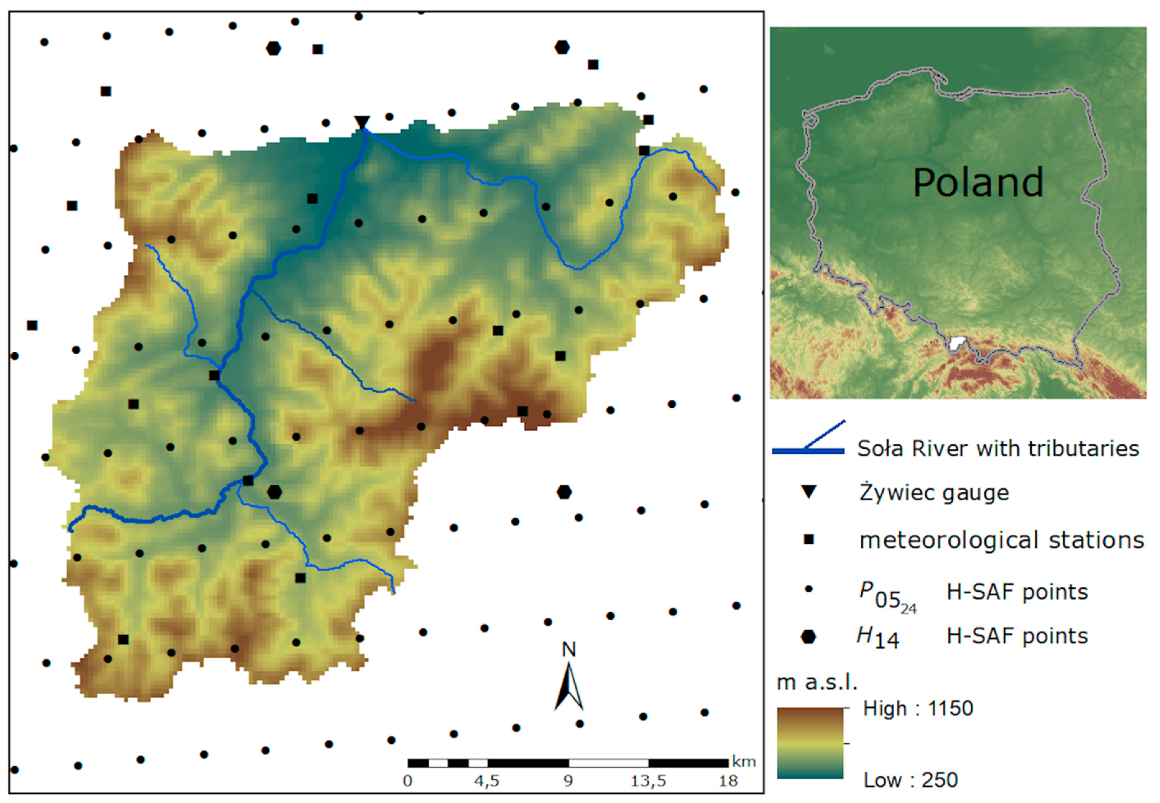
2. Study Area and Data

The Sola River in Poland, the Vistula River’s first major tributary, extends 88.9 $\mathrm{km}$ (55.24 miles) within the Sola Watershed. The watershed, which covers an area of 1400 km² (540.543 sq. mi.) (19.23°–22.68° E, 50.05°−53.71° N; Figure 1), is monitored by the Zywiec gauging station. Roughly two-thirds of the regional annual precipitation ($P_{\mathrm{ann}}$), which varies from 750 to 1300 mm year⁻¹, occurs between May and October, with 39% of $P_{\mathrm{ann}}$ occurring during the three summer months (June–August) and 17% falling in the winter months (December–February) [37]. Accordingly, high water levels occur primarily in March and April due to the spring snow-melt, and in July and August due to storm rainfall. The same factors that lead to high peak flood levels also result in shorter peak flow levels. Generally, the Sola Basin experiences flash floods during the summer months.

The rain gauge measurements used in the validation of the BC method and the Kalman filter procedure were obtained from Poland’s Institute of Meteorology and Water Management—National Research Institute (IMWM—NRI). H-SAF-derived precipitation and soil moisture products were generated from the rain gauge data. Observed daily precipitation data, $P_{\mathrm{OBS}}$, were obtained for the period of July 2012 to May 2015. The locations of the ground-based IMWM−NRI meteorological stations (black squares, Figure 1), and precipitation H-SAF product readings (black points, Figure 1) in the Sola Watershed highlight the difference in the grid of H-SAF products, $P_{{05}_{24}}$ vs. $P_{\mathrm{OBS}}$.

The $P_{{05}_{24}}$(mm) observation was derived from precipitation maps generated by merging microwave detector (MW) images from operational sun-synchronous satellites, and infrared (IR) images from geostationary satellites. Sampling was performed using the Spinning Enhanced Visible and Infrared Imager Instantaneous Field of View (SEVIRI IFOV) instrument, i.e., a line by line scanning radiometer, which provides image data in four Visible and Near InfraRed (VNIR) channels and eight InfraRed (IR) channels. In order to minimize bias and random errors, the satellite-derived field was forced to integrate precipitation intensities and some information sources, such as rain gauge data and quantitative precipitation forecasts (QPF) from a Numerical Weather Prediction (NWP) model [38]. Integration was performed over 3, 6, 12 and 24 h, and $P_{{05}_{24}}$, or accumulated precipitation, over 24 h, was selected for analysis. The $P_{{05}_{24}}$ resolution for the Sola Catchment changes from 3.5 km horizontally to 5.9 km vertically (Figure 1).

With respect to the H-SAF products, SM-DAS-2 (or $H_{14}$) at the root zone level, i.e., the soil moisture index $I_{\mathrm{rz}\mathsf{\theta }}$, was generated in the ECMWF Land Data Assimilation System by assimilating ASCAT soil moisture data [39]. The value of $H_{14}$(%) was a result of land surface analysis that included screen level parameters (2 m) from surface synoptic observations and soil moisture analysis based on a simplified extended Kalman filter.

The primary ASCAT observation, sea-surface wind, was processed at a 50 km resolution. Soil moisture data processing was performed at a 50 km resolution in operational mode (verified products for operational hydrological applications) and a 25 km resolution in research mode (products developed pre-operationally). The resolution of the H₁₄ soil moisture products in the Sola Basin changes from 16.287 km horizontally to 25.07 km vertically (black hexagon, Figure 1).

The ECMWF model-generated soil moisture profiles, according to the Hydrology Tiled ECMWF Scheme for Surface Exchanges over Land, provides estimates for four layers (for a total thickness of 2.89 m), with a daily time step. The soil moisture-related products constitute the inputs into the mathematical model, representing a vertical profile of the following soil depth ranges: $0 –0.07$ $\mathrm{m}$, $0.07 –0.28$ $\mathrm{m}$, $0.28 –1.00$ $\mathrm{m}$ and $1.00 –2.89$ $\mathrm{m}$. In keeping with the inputs of the HBV hydrological model, the $H_{14}$ product was simplified by calculating a weighted average of the first three or four depths considered ($0 –1.00 \mathrm{m}$, $H_{14}^{1.00}$ and $0 –2.89 \mathrm{m}$, $H_{14}^{2.89}$, respectively). In order to perform the BC procedure it was necessary to generate a sequence of soil moisture values using HBV, ${\theta }_{\mathrm{HBV}}$ (mm) with the same range as the employed satellite data. In the BC scheme, the soil moisture ${\theta }_{\mathrm{HBV}}$ must be expressed in %, like the $H_{14}$. Therefore, the ${\theta }_{\mathrm{HBV}}$ was recalculated according to the formula: ${\theta }_{\mathrm{HBV}}(\%)$= $\left[\frac{{\theta }_{\mathrm{HBV}}\left(\mathrm{mm}\right)}{F\mathrm{c}}\right]100$%, where F_C is the soil water capacity, a state variable of the HBV, with a value determined during HBV calibration. After applying the developed BC scheme to compute the Kalman gain, the values of θ (%) were recalculated as follows:

$$\theta \left(\mathrm{mm}\right)=\left[\frac{F_{\mathrm{c}}\left(\mathrm{mm}\right)\theta (\%)}{100\%}\right]$$

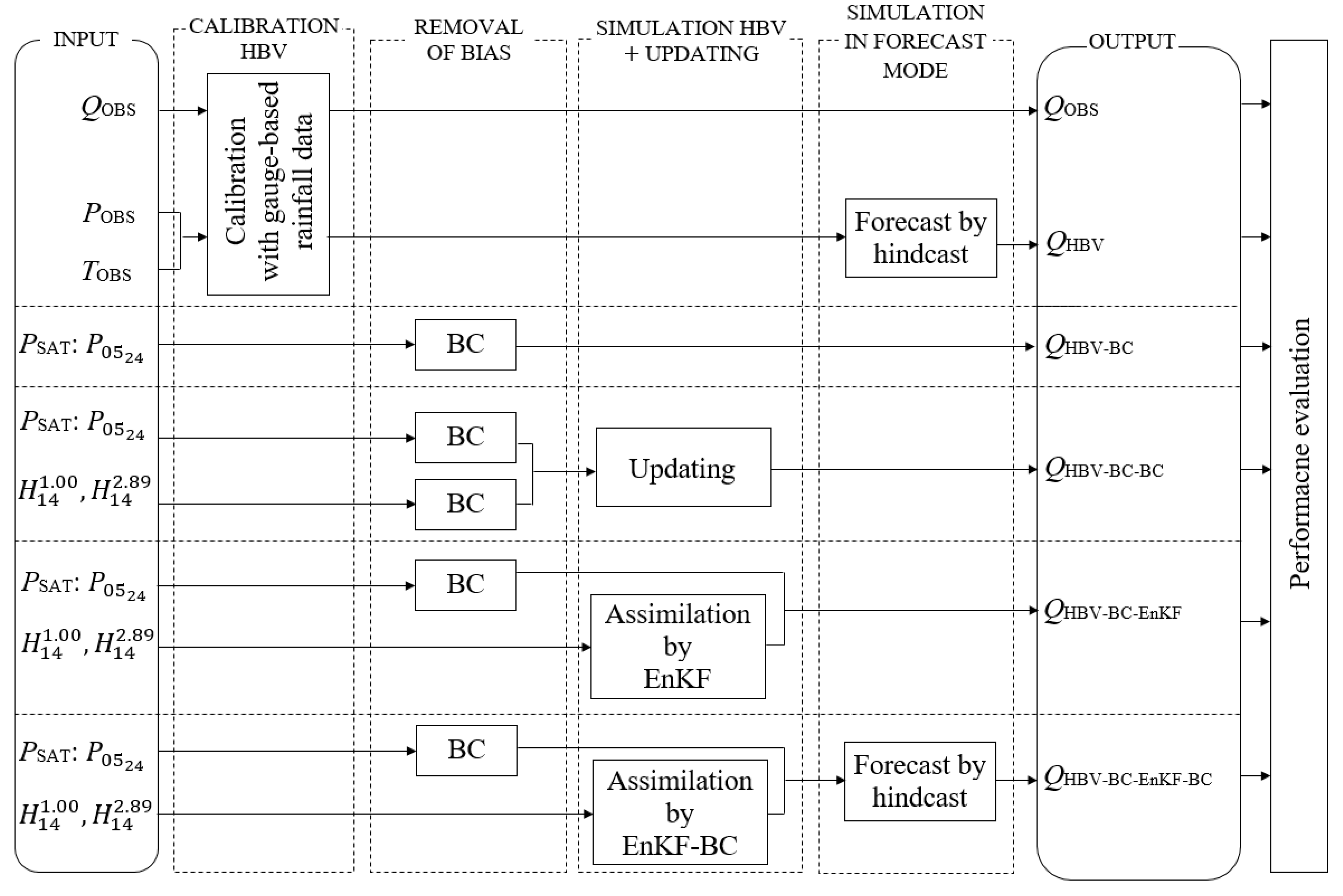
3. Problem Formulation and Methodology

In the current study, the ensemble Kalman filter (EnKF) and ensemble Kalman filter with bias correction (EnKF-BC), were used with bias correction (BC) and assimilation methods, to develop a procedure that was dynamically coupled with the Hydrologiska Byråns Vattenbalansavdelning (HBV) model. The proposed methodology (vertical columns, Figure 2) is a composite of four substantive modules, with the possibility of configuring the computational component with regards to input, output and performance evaluation. The methodology can be described as follows:

• Calibration of the deterministic HBV hydrological model based on observations and measurements from the hydro-meteorological monitoring network of the IMWM—NRI;
• Removal of bias from the satellite precipitation product, $P_{\mathrm{SAT}}$: $P_{{05}_{24}}$, and from satellite soil moisture observations, $H_{14}$: $H_{14}^{1.00}$ and $H_{14}^{2.89}$, using the BC method in all phases (e.g., probability distribution fitting, validation and correction);
• Simulation of the HBV model with and without the updating procedure. The HBV model was updated using three methods:
  • Bias correction $H_{14}^{1.00-\mathrm{BC}}$ or $H_{14}^{2.89-\mathrm{BC}}$ without assimilation (the bias-corrected satellite observations replaced the proper state variables of the HBV),
  • Assimilation of the uncorrected satellite soil moisture data, i.e., $H_{14}^{1.00}$ or $H_{14}^{2.89}$, using EnKF, and
  • Assimilation of the uncorrected satellite soil moisture data, i.e. $H_{14}^{1.00}$ or $H_{14}^{2.89}$, with the bias correction of the perturbed background prediction of soil moisture, for the creation of an unbiased ensemble of model states using EnKF-BC.
  These three methods use $P_{{05}_{24}}^{\mathrm{BC}}$ as the precipitation input (i.e., a forcing data),
• Simulation in forecast mode in the form of an ensemble (interval forecast) using the hindcast method, in which the input (forcing data) of the hydrological model is the historical data instead of the meteorological forecast data, e.g., $P_{\mathrm{OBS}}$, observed ground-based precipitation and $T_{\mathrm{OBS}}$, temperature.

The inputs were: River discharge ($Q_{\mathrm{OBS}}$), observed ground-based precipitation ($P_{\mathrm{OBS}}$), temperature ($T_{\mathrm{OBS}}$) and satellite observations (i.e., precipitation products, $P_{\mathrm{SAT}}$: $P_{{05}_{24}}$ and soil moisture observations, $H_{14}$: $H_{14}^{1.00}$ and $H_{14}^{2.89}$). Depending on the inputs, the methodology adopted in this work evaluates the performance of five different simulations. In the first step, the calibration of the HBV model with gauge-based rainfall data was initiated. The steps used to calibrate the HBV model are discussed in depth in the following sections. The appropriate configuration allowed for the generation of the following outputs: $Q_{\mathrm{HBV}-\mathrm{BC}}$ (river discharge calculated by the HBV model with input in the form of corrected satellite precipitation, without the assimilation method), $Q_{\mathrm{HBV}-\mathrm{BC}-\mathrm{BC}}$ (updating the HBV model using bias-corrected $H_{14}^{1.00-\mathrm{BC}}$ or $H_{14}^{2.89-\mathrm{BC}}$ without assimilation), $Q_{\mathrm{HBV}-\mathrm{BC}-\mathrm{EnKF}}$ (updating the HBV model with the assimilation of uncorrected satellite soil observations by EnKF filter), and $Q_{\mathrm{HBV}-\mathrm{BC}-\mathrm{EnKF}-\mathrm{BC}}$ (updating the HBV model with the assimilation of uncorrected satellite soil moisture observations by EnKF-BC filter).

3.1. Calibration of the Deterministic HBV Hydrological Model

The conceptual rainfall-runoff HBV model (version HBV 7.3) [40,41,42,43] was used to model rainfall and runoff patterns in the Sola Basin. The HBV model is a partially-distributed conceptual rainfall-runoff model that uses simple continuity equations and other supplementary relationships to simulate streamflow in gauged or ungauged rivers, to design flood calculations and to perform hydrological forecasting. The model consists of sub-routines for snow accumulation and snowmelt, soil moisture, runoff generation and simple routing. The main control of runoff formation in the rainfall-runoff HBV model is the soil moisture accounting routine: When the soil is dry, the runoff from rain or snowmelt is small, whereas when the soil is wet, the runoff is higher. Therefore, the runoff generation routine is the response function that transforms excess water from the soil moisture layer to the runoff.

The structure of the HBV system allows the model to make necessary sub-divisions concerning different climate zones, land-use types, hydro-meteorological network densities and other variables. In this study, a hydrologic analysis of the study area was attempted without dividing the area into sub-catchments. The model used a lumped scheme, setting up the catchment as a single vegetation zone, i.e., a field area [44], thus the simulation carried out a single soil moisture box with lumped inputs. As a consequence of the lumped scheme, the satellite products from a regular satellite grid ($H_{{05}_{24}}$,$H_{14}^{1.00}$, $H_{14}^{2.89}$) and from irregular ground-based meteorological stations ($P_{\mathrm{OBS}}$) were spatially interpolated into the centroid of the Sola Watershed’s catchment. In the present study, the simple Thiessen polygons interpolation technique was used [45].

The HBV model was treated solely as a calibrated engine, i.e., as a dynamic function of the HBV, and the model was assumed to have its own set of initial state variables, constants and definitions. A relatively long period of ground-based meteorological station observations (from 1 January 2008 to 31 July 2014) was used to calibrate the model. This was done automatically with small manual corrections for the following model parameters: Field capacity, limit for potential evaporation, exponent in the formula for soil drainage, recession coefficient and precipitation and snow melt factors. It was further assumed that the model was well-calibrated, such that it did not require additional adjustments during assimilation run-up, i.e., the hydrological model was not re-calibrated with input data derived from satellite-based products.

3.2. Bias Correction of Ground-Based Observations and Satellite Products—The Distribution Derived Transformation Method

The BC algorithm was tested for its ability to remove bias from satellite precipitation and soil moisture data series. Several methods for downscaling and correcting bias in monthly and daily data derived from hydro-meteorological models have been proposed [46,47,48], and applied to satellite-based remotely-sensed data [9,10,11]. However, associating the downscaled data drawn from different sources (e.g., weather data, mathematical climate model outputs, radar or satellite remote sensing data) with the appropriate input of hydrological models can be problematic. Generally, the correction methods applied to meteorological data fall into four main categories [49]: (i) Methods based upon simple changes in data attributes/values [5]; (ii) parametric transformations [6,50,51]; (iii) non-parametric transformations [11,52]; and (iv) distribution-derived transformations [8,36,53,54,55].

In the current study, the method of transforming the derived distribution (iv) was selected for the removal of systematic differences between observed and modeled satellite H-SAF products. In the case where the marginal distribution of the variable of interest was known, the transformation was achieved using the theoretical distributions to solve the equation [8]:

$$X_{\mathrm{OBS}}=F_{\mathrm{OBS}}^{-1}\left(F_{\mathrm{MOD}}\left(X_{\mathrm{MOD}}\right)\right)$$

(1)

where:

$F_{\mathrm{MOD}}$ is the cumulative distribution function (CDF) of the modeled variable $X_{\mathrm{MOD}}$, and

$F_{\mathrm{OBS}}^{-1}$ is the inverse CDF corresponding to the observed variable, $X_{\mathrm{OBS}}$.

The Bernoulli distribution (B) was used to model the precipitation occurrence probability, while the gamma (GA) theoretical distribution was used for modeling intensities [36].

Joined distribution in pairs, including the Bernoulli-Weibull (B-WE), Bernoulli-lognormal (B-LN) and Bernoulli-exponential (B-E) distributions [54], were also used. As previously mentioned, gamma-gamma (GA-GA) transformation is typically used for similar applications [6,8].

In the current study a distribution-derived transformation method with a new algorithm using three theoretical distributions with similar random properties was developed. Generalized exponential (GE), gamma (GA) and Weibull (WE) distributions were used separately, or in paired combinations (e.g., GE-GA, GE-WE, etc.) to generate bias-free satellite precipitation and soil moisture data (see details in Appendix A).

Satellite precipitation data (i.e., $P_{{05}_{24}}$) were compared with $P_{\mathrm{OBS}}$ from ground-based meteorological stations, while satellite soil moisture observations (i.e., $H_{14}$) were compared to the value of ${\theta }_{\mathrm{HBV}}$ derived from the HBV model. Certain variable boundaries were assumed for each variable (P meaning precipitation and θ meaning soil moisture):

$$P=\{\begin{array}{c}P P\ge 0.1 \mathrm{mm}\\ 0 P<0.1 \mathrm{mm}\end{array}; \theta =\{\begin{array}{c}\theta 100\ge \theta >0 \% \\ 100 \theta >100 \% \\ 0 \theta \le 0 \% \end{array}$$

(2)

Within the BC method the satellite products were processed through fitting probability distributions to $P_{\mathrm{OBS}}$ and ${\theta }_{\mathrm{HBV}}$, and subsequently validated. Model performance comparisons are discussed in depth in Section 3.4. Subsequently, corrected satellite precipitation, $P_{{05}_{24}}^{\mathrm{BC}},$ was used as a direct input into the HBV simulation (a forcing data), and $H_{14}^{1.00-\mathrm{BC}}$ and $H_{14}^{2.89-\mathrm{BC}}$ were used as direct inputs into the HBV simulation without assimilation (as part of a simple updating procedure for the HBV model, the corrected satellite soil moisture observations were directly substituted for the corresponding HBV state variable). Probability distribution fitting of the BC model for soil moisture provided optimized parameter functions that transformed each observation into its corrected form. Information on the optimal probability distributions helped to correct the soil moisture for unbiased perturbing within the Kalman filter procedure.

Distribution fitting data for the bias correction procedure of $P_{{05}_{24}}$ were drawn from 1 January 2013 to 31 July 2014, while data for $H_{14}^{1.00}$ and $H_{14}^{2.89}$ were drawn from 1 January 2012 to 31 July 2014. All validation data were drawn from 1 August 2014 to 30 April 2015. Input ranges for the calibration of the HBV model and BC method were different, and depended upon the period in which the data were observed/measured. Distribution fitting and validation of $H_{14}^{1.00}$ and $H_{14}^{2.89}$ took into account the summer (August to October) and winter (November to April) seasons. In Poland, the hydrological division is represented by two seasons: Winter starts on 1 November and ends on 30 April, and the remaining period is considered the summer season. Such a division of time agrees with the course of the drain cycle phenomena. Climatic winter begins in one of the last two months of the year, and the outflow of rainwater, made difficult in winter due to freezing temperatures, takes place only during the spring months of the following calendar year.

The corrected satellite products from 1 August 2014 to 30 April 2015 then served as the input for the hydrological simulation model. The results of the distribution fitting and validation of the bias correction procedure are discussed in Section 4.2.

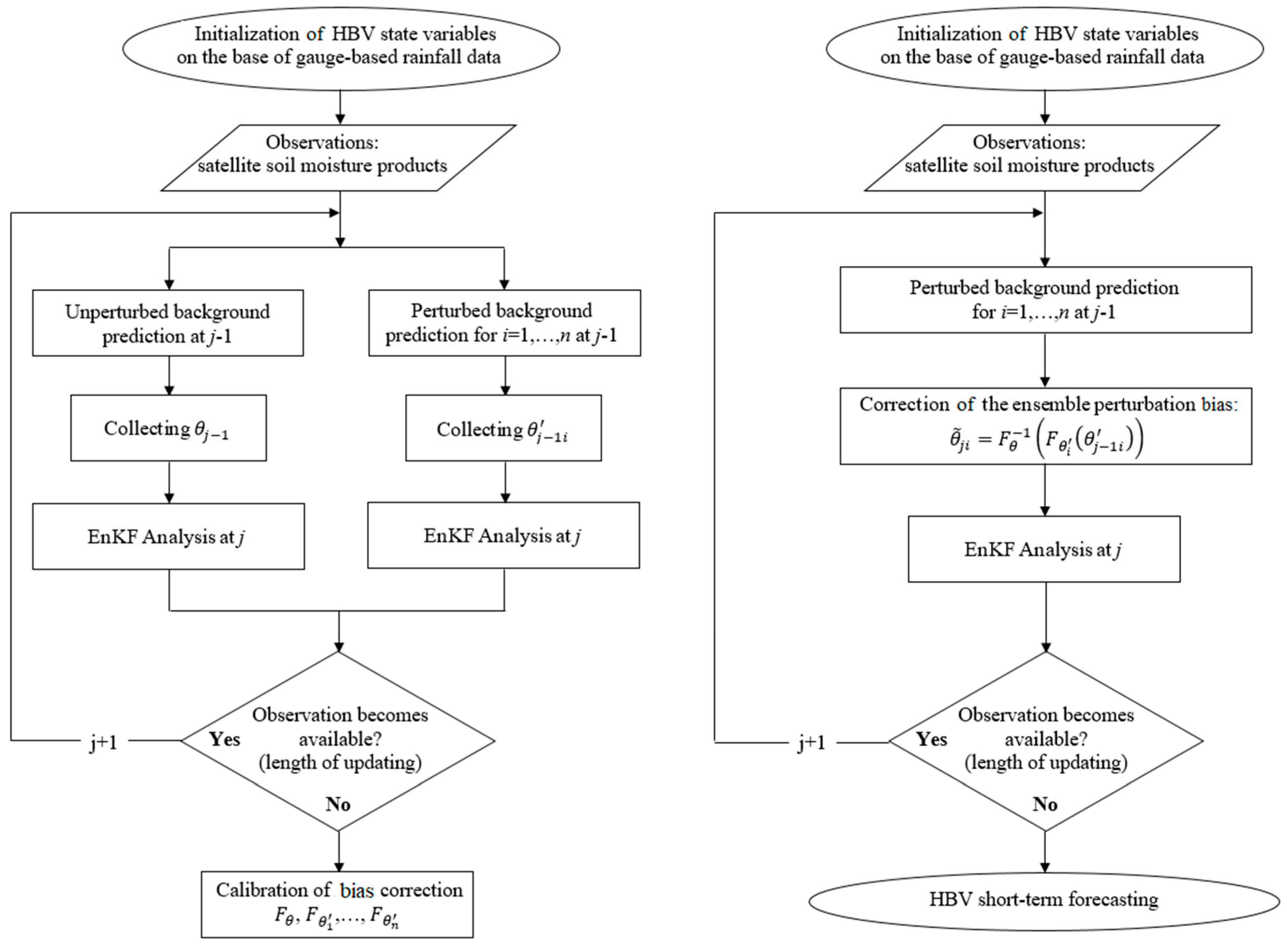
3.3. Assimilation of Satellite Products Using the Ensemble Kalman Filter

The data assimilation approach employed in the present study was based on the EnKF technique. The Kalman filter is considered the most efficient sequential DA scheme, as it only requires: (i) System variables of a previous time step and forcing terms and (ii) observations from the current time step [12]. This filter also provides powerful support for estimations of past, present and future states via a set of mathematical equations that provide an efficient computational framework that can estimate the state of a process, while minimizing the mean of the squared error [56].

The EnKF is derived from the standard Kalman filter [57] and generates ensembles ipso facto, extending the sampling range to account for the model and forcing uncertainties in the presence of non-linear processes. For the EnKF method, model errors and uncertainties are assumed to be Gaussian distributed when all uncertainties are defined.

Such a situation, however, is rare in hydrological datasets. Most of the existing data assimilation techniques, including the EnKF, have been developed to correct random error that occurs, but systematic errors must be removed separately. It is important to update the soil moisture state variable; however, soil moisture estimates from DA are sensitive to observations and model error variances. Estimated state variables with high input errors can prove to be far less accurate than DA-free model estimates. For simulations of non-linear and non-Gaussian relationships between model states and observations, one can use the EnKF. However, the possibility of bias introduction in the estimations of non-linear processes must be considered in the analysis.

In this study, the hydrological model HBV was run forward in time with a finite set of ensemble members. In the EnKF, the model error estimates were produced assuming that the ensemble mean was correct. The variance of the differences between ensemble members and the ensemble mean were then calculated. Model error was estimated directly from the ensemble. Each observation was updated based on the relative error between the model and observations. The update of the model states with the EnKF filter assumed that model errors had a Gaussian distribution (see Appendix B for the detailed mathematical formulation).

One weakness of the EnKF is the occurrence of errors resulting from the use of perturbed observations. The resulting noise added to the perturbed observations can be correlated with the background error. This can result in a systematic underestimation of the analysis error variance [58].

3.3.1. Model Error and the Perturbation of Error Factors within the EnKF Filter Algorithm

Model errors can result from uncertainties in model inputs (forcing data), model structure and model parameters [33,59]. These errors represent unbiased noise, which adds to forcing variables, model state variables and/or model parameters. In this study, a problem appeared when applying unbiased perturbations to the soil moisture variable. The unperturbed background prediction was designated as θ, while the perturbed state was represented as ${\theta }^{\prime }$ to simplify the computational formulas. Similarly, the unperturbed and perturbed precipitation were defined as P and $P^{\prime }$, respectively. In their study, Alvarez-Garreton et al. [33] ensured that the ensemble of model states remained unbiased after perturbation by implementing the BC scheme proposed by Ryu et al. [34]. Furthermore, the authors applied a post-processing technique that involved the simultaneous run of a hydrological model with and without the perturbation of state variables. The mean bias of the perturbed state variables of n ensemble members at the time j (δ_j) was computed by subtracting the unperturbed background prediction (${\theta }_j$) from the ensemble mean of the perturbed states [34], as follows:

$${\delta }_j=\frac{1}{n}{\displaystyle \sum }_{i=1}^n\left({\theta }_{j-1}^{\prime }-{\theta }_j\right)$$

(3)

where ${\mathsf{\delta }}_j$ is the mean bias of the perturbed state variables of n ensemble members at the time j.

In order to obtain an unbiased ensemble of state variables (${\tilde{\theta }}_{j,i}$) (i.e., a corrected ensemble), the perturbation bias (δ_j) was subtracted from the perturbed ensemble states (${\theta }_{j-1,i}^{\prime }$) [34]:

$${\tilde{\theta }}_{j,i}={\theta }_{j-1,i}^{\prime }-{\mathsf{\delta }}_j$$

(4)

Since soil moisture is expressed as a percentage ranging from 0% to 100%, the application of Gaussian noise during assimilation using the EnKF often violates this constraint. To avoid crossing these limits while generating the variance of the noise term (${\xi }_{\theta }~\mathrm{N}\left(0,{\sigma }_{\theta }^2\right)$), where ${\sigma }_{\theta }^2$ is the standard deviation of the normal distribution, Baguis and Roulin [35] used truncated normal probability distributions to impose upper (100) and lower (0) boundaries on the soil moisture products variable. Similarly, they used the truncated log-normal distribution to generate the perturbation for the precipitation variable. For the random variable, X, with the function of density, f, and the cumulative distribution function, F, the interval limit (a, b] is described by the distribution function, g(f)_{(a, b]}, according to the formula [60]:

$$g{\left(f\right)}_{\left(a,b\right]}\left(x\right)=\frac{f\left(x\right)}{F\left(b\right)-F\left(a\right)}$$

(5)

where,

$$f\left(x\right)=\{ \begin{array}{c}f\left(x\right) a<x\le b \\ 0 x\le a {{\displaystyle \cup }}^{} x>b \end{array}$$

(6)

for a = 0% and b = 100%.

The current study adopted a multiplicative error model for rainfall data [59]. The precipitation error was expressed as ${\xi }_p~\mathrm{lnN}\left(1,{\sigma }_p^2\right)$, where ${\sigma }_p^2$ was the standard deviation of the log-normal distribution. For the soil moisture error, a simplified model was used and expressed as ${\xi }_{\theta }~\mathrm{N}\left(0,{\sigma }_{\theta }^2\right)$. In practice, under the EnKF method, DA was preceded by a calibration involving a sensitivity analysis of user-selected state variables, and the values of observation errors were set within a specified allowable range. For example, fractional error parameters were proposed for the EnKF method as ξ_θ = 0.20 and ξ_P = 0.10. These errors were chosen based on the sensitivity analysis using the following acceptable sets: 0.10 ≤ ξ_θ ≤ 0.40 and from 0.05 ≤ ξ_P ≤ 0.40.

As only one variable was assimilated from the satellite observations (H₁₄, i.e., $H_{14}^{1.00}$ or $H_{14}^{2.89}$) in this research, the assimilation problem was one-dimensional, and all the matrices included were real numbers (see Appendix B for more information on the DA algorithms used for model state updating).

Optionally, ensembles can be produced by stochastically perturbing the precipitation, P, and soil moisture, θ [59]. In implementing the EnKF, it was assumed that θ was perturbed by default, though the choice of $P_{{05}_{24}}$ was up to the user’s discretion. $P_{{05}_{24}}$, as a forcing data, should be perturbed when the dynamic HBV function generates an outflow that is significantly different from the observed outflow. The HBV model was run with an hourly step, while the satellite soil moisture was only available at a daily step. In the implemented Kalman filter procedure, the soil moisture model was updated if the product, $H_{14}$, was available.

The perturbations were parameterized as fractional error parameters for ξ_θ and ξ_P and were related to $\theta$ and P. Soil moisture (θ) was accordingly defined as:

$${{\theta }^{\prime }}_{ji}~{\theta }_j+\mathrm{U}\lfloor -{\xi }_{\theta }\left({\theta }_j-{\theta }_{j-1}\right); +{\xi }_{\theta }\left({\theta }_j-{\theta }_{j-1}\right)\rfloor {\xi }_{\theta }=\left\{0.1, \cdots ,0.4\right\}$$

(7)

where:

• ${{\theta }^{\prime }}_{ji}$ was the perturbed ${\theta }_j$, i.e., the soil moisture storage for the ith ensemble member, for $j=1,\dots N$, where $N$ is the number of simulation steps, and for $i=1, 2, \cdots , n$, where n is the size of the ensemble assumed in the procedure,
• ${\theta }_j$ is the soil moisture storage in the j^th step,
• ${\theta }_{j-1}$ is the soil moisture storage calculated in the previous (j − 1)^th step and
• U is the uniform distribution in the range of ±${\xi }_{\theta }\left({\theta }_j-{\theta }_{j-1}\right)$.

Precipitation, P, was defined as:

$${P^{\prime }}_{ji} ~P_j+\mathrm{U}\lfloor -{\xi }_P{P}_j; +{\xi }_P{P}_j\rfloor {\xi }_P =\left\{0.05, \cdots , 0.40\right\}$$

(8)

where:

• ${P^{\prime }}_{ji}$ is the perturbed $P_j$ precipitation for the i^th ensemble member, for $j=1,\dots ,N$ and for $i=1, 2, \cdots , n$,
• $P_j$ is the input areal average precipitation from the measurement and observation network in the j^th step, and
• U is a uniform distribution in the range $\pm {\xi }_P{P}_j$.

3.3.2. A New Procedure for the EnKF Coupled with the Bias-Correction Scheme Using Distribution-Derived Transformation

Within EnKF, a BC scheme (Section 3.2.) was applied to the soil moisture background prediction. The proposed BC scheme was a post-processing technique (Figure 3). This procedure, in contrast to the method of Ryu et al. [34], takes into account the distribution of bias of the perturbed state variable of the n ensemble members at the time j, not just the mean bias. Specifically, this study used the distribution-derived transformation technique for the removal of bias.

The procedure was divided into two stages: A probability distribution fitting of the bias correction method (left part of Figure 3), and a correction of the ensemble perturbation bias within the EnKF-BC filter (right part of Figure 3). Input to the distribution fitting of the BC scheme (left part of Figure 3) for unbiased perturbations was a random sample of two variables, $\theta$ and ${\theta }^{\prime }$, representing the unperturbed and perturbed background prediction of soil moisture, respectively, where $\theta =\left\{{\theta }_j\right\}$ and ${\theta }^{\prime }=\left\{{\theta }_{ji}\right\}$ for $j=1,\dots ,N$ and for $i=1,\dots ,n$. The above procedure required parallel simulation with and without the perturbed ensemble states (left part of Figure 3). Within the distribution fitting of the distribution-derived transformation method [8] (separately for $\theta$ and ${\theta }_i^{\prime })$, an optimal theoretical marginal distribution was chosen, i.e., $F_{\theta }$ and $F_{{\theta }_1^{\prime }},\dots ,F_{{\theta }_n^{\prime }}$ (see Appendix A). Based on the results of the calculations described in Section 3.2, the considerations were limited to one theoretical probability distribution. The size of the random sample (i.e., from 1 January 2012 to 31 July 2014, dividing into the summer, from 1 May to 31 October, and winter from 1 November to 30 April, with a daily step) was sufficient to obtain optimal theoretical distributions two seasons. The probability distributions (i.e., type of distributions and parameters) were necessary to carry out the correction of the ensemble perturbation bias within the EnKF-BC filter. $F_{\theta }$ and $F_{{\theta }_1^{\prime }},\dots ,F_{{\theta }_n^{\prime }}$ were inputs into the EnKF-BC within the HBV updating procedure using assimilation by EnKF-BC from 1 August 2014 to 30 April 2015, including summer and winter seasons (right part of Figure 3).

It was assumed that the random properties of the ensemble state variables would be subject to the above estimated probability distributions during the simulation of the HBV model with updating. The assumption that the modeled relation holds if confronted with new data [49] is intrinsic to statistical transformations. The above assumption can be addressed in the context of the perturbation technique by using a uniform distribution. The distribution-derived transformation showed relatively poor performance with respect to the extreme part of the distribution. The theoretical form of the transformation equation, however, was relatively easy to calibrate (optimize) and convenient to implement, which is an important feature in this application.

Thus, a bias-corrected ensemble of state variables (${\tilde{\theta }}_{ji}$) was calculated as:

$${\tilde{\theta }}_{ji}=F_{\theta }^{-1}\left(F_{{\theta }_i^{\prime }}\left({\theta }_{j-1i}^{\prime }\right)\right)$$

(9)

where:

• $F_{\theta }$,$F_{{\theta }_1^{\prime }},\dots ,F_{{\theta }_n^{,}}$ are the cumulative distribution functions (CDF) of the unperturbed and perturbed background prediction of the soil moisture variable, $\theta$, and
• $F_{\theta }^{-1}$ is the inverse CDF corresponding to the unperturbed variable, $\theta$.

The physical limits of this variable (lower and upper bounds) were taken into account within the bias correction procedure (Equation (2)).

3.3.3. Scheme of the KF Method Used in the Assimilation Procedure

The assimilation of satellite products was divided into two periods: Summer (1 August to 31 October 2014) and Winter (1 November 2014 to 30 April 2015). The summer season started on 1 August, and not on May 1, due to a lack of hourly river discharge observations at the gauge. This seasonal division was implemented to account for the occurrence of air temperatures below 0 °C, and permanent snow cover in the cold season. This division allowed for the examination of the effects of seasonal change on the assimilation of the satellite products, especially with regards to ${\theta }_{\mathrm{HBV}}$. The assimilation procedure is a continuous process, which, in this study, uses different distribution-derived transformation equations (BC) determined for the summer and winter season during the calibration of EnKF-BC (left part of Figure 3). The BC method can use various types of probability distributions and parameters, which were estimated during the calibration procedure of EnKF-BC.

A scheme of the KF method used in the assimilation procedure, including the EnKF-BC, shows how this method, integrated into the form of a dynamic HBV function, allowed for updating with partial sequences of the observed soil moisture (right part of Figure 3). The proposed algorithm for the assimilation of satellite soil moisture products started with the initialization of HBV model parameters. The set of perturbed background predictions, the ensemble corrected bias perturbation and the observations pseudo in situ of the satellite products, were then used as inputs to the EnKF analysis. The EnKF analysis included: (i) Simulation ensembles to obtain new forecasted data and to run the HBV model for each ensemble member; (ii) calculation of the Kalman gain (K); and (iii) updating of the ensemble members using K. The calculation of K included θ (mm), the soil moisture background state variable.

The EnKF method of assimilation involved choosing the size of the ensemble (n was the number of members) while allowing for sufficient time to process the annual hydrographs (BC of the perturbed ensemble state variables as a post-processing technique).

While a total ensemble size of $10-100$ members was tested, the number of members per ensemble was set to 10. The basic criterion for choosing the size of the ensemble was the short processing time, while guaranteeing an even distribution of perturbed hydrographs throughout the entire ensemble. Assimilation was ongoing, as long as new observations of satellite soil moisture were available.

A hindcasting method was used to test the predictive HBV hydrological model, taking into account the updating procedure using DA, i.e., the EnKF-BC. In the last step of updating, n vectors of updated state variables were obtained. Next, the HBV model was run (in forecasting mode) with existing historical hourly data (forcing data) as an input (i.e., $P_{\mathrm{OBS}}{}_{+1}, \cdots , P_{\mathrm{OBS}}{}_{+72}, \mathrm{and} T_{{\mathrm{OBS}}_{+1}}\cdots , T_{{\mathrm{OBS}}_{+72}} ).$ The simulation in forecasting mode did not perform the DA procedure. This revealed how well the output matched the known results. Optionally, in the first step of the simulation run in the forecasting mode, a total of $m$ perturbations for n = 10 ensemble sets of state variables obtained in the last step of updating could be allowed. Theoretically, the width of the forecasted ensemble (interval forecast) could reach a size equal to $n \times m$. It was assumed that the forecasts generated by the HBV model with the previous updating would be presented as a single hydrograph of an average ensemble of flows ($Q_{{\mathrm{HBV}}_{+1}},\dots ,Q_{{\mathrm{HBV}}_{+72}}$) and ensemble hydrographs.

3.4. Model Performance Comparison

The validity of the selection of the optimal theoretical marginal distributions for both historical (observed) and modeled (satellite precipitation and soil moisture products) variables was assessed using the Akaike Information Criterion (AIC) [61], while the model performance evaluation was based upon the following parameters:

• ${\mathrm{R}}_0\mathrm{M}$ showing over (${\mathrm{R}}_0\mathrm{M}>1.0$), under (${\mathrm{R}}_0\mathrm{M}<1.0$) or perfect (${\mathrm{R}}_0\mathrm{M}=1.0$) prediction of the desired parameter [62].

  $${\mathrm{R}}_0\mathrm{M} =\frac{\frac{1}{n}{{\displaystyle \sum }}_{i=1}^{i=n}{P}_i }{\frac{1}{n}{{\displaystyle \sum }}_{i=1}^{i=n}{O}_i }=\frac{\overline{P}}{\overline{O}}$$

  (10)

  where:
  • n is the number of modeled (corrected) values,
  • $O_i$ is the i^th observed value,
  • $\overline{O}$ is the mean of the observed values,
  • $\overline{P}$ is the mean of the predicted values and
  • $P_i$ is the i^th predicted value.
• $\mathrm{RMSE}$, a scale-dependent measure of accuracy for assessing different models’ ability to predict a single variable [63], was expressed in $\mathrm{mm}$ for satellite precipitation and pseudo in situ observations of soil moisture, and as ${\mathrm{m}}^3{\mathrm{s}}^{-1}$ for the procedure product,
• the Nash-Sutcliffe Model efficiency index ($\mathrm{EI}$) [64], where $-\infty <\mathrm{EI}\le 1.0$, with $\mathrm{EI}=1.0$ representing a perfect match between observed and predicted values, and $\mathrm{EI}\le 0$ representing a prediction no better than the mean of observed values. Values of $\mathrm{EI}\ge 0.5$ were taken to represent a satisfactory model performance.

4. Results and Discussion

4.1. Selecting the Best Probability Distribution Function for $P$ and $\theta$ Based on the AIC

Based on minimizing AIC values [61], one of three probability distribution functions (GE, GA or WE) with three parameters (α, β and ε, Equation (1)–Equation (3) in Appendix A) was deemed to best fit the studied variable’s distribution (

Table 1. Choice of the distribution used in the bias correction of precipitation and soil moisture H-SAF products: $P_{{05}_{24}}$, $H_{14}^{1.00}$ and $H_{14}^{2.89}$ based on the AIC (Akaike Information Criterion) with: WE (Weibull), GA (gamma) and GE (generalized exponential) distribution. Bolded values represent the best fitting distributions.

Product		Distribution				AIC
		Type	Coefficients
			A	β	ε
Precipitation
$P_{\mathrm{OBS}}$		WE	0.0091	0.3389	0.0990	9673.47
		GA	0.9979	0.2313	0.0000	9702.60
		GE	1.2140	4.9784	0.0000	9520.16
$P_{{05}_{24}}$		WE	0.0130	0.3239	0.0990	8134.90
		GA	0.7193	0.1824	0.0540	21895.00
		GE	1.8952	8.2915	0.0000	15248.30
Soil Moisture
Winter Season	${\theta }_{\mathrm{HBV}}$	WE	34.4556	5.6428	38.00	4549.28
		GA	69.1987	1.0107	0.00	4709.36
		GE	11.3523	0.0885	36.00	5102.45
	$H_{14}^{1.00}$	WE	20.6861	4.0103	42.40	4212.17
		GA	50.8409	0.8123	20.00	4186.79
		GE	12.1816	0.1415	40.00	4502.38
	$H_{14}^{2.89}$	WE	40.6269	3.8497	19.80	5178.59
		GA	19.8836	2.8677	0.00	5250.16
		GE	5.9666	0.0631	18.60	5572.46
Summer Season	${\theta }_{\mathrm{HBV}}$	WE	33.2265	2.9743	22.80	4954.12
		GA	20.0311	2.6243	0.00	4982.81
		GE	9.6627	0.0820	18.00	5110.21
	$H_{14}^{1.00}$	WE	17.8183	2.9249	46.50	4173.68
		GA	61.1260	0.7925	14.00	4165.42
		GE	8.2893	0.1502	44.50	4324.50
	$H_{14}^{2.89}$	WE	26.5781	4.6010	38.80	4253.31
		GA	66.0066	0.8109	9.60	4197.62
		GE	28.7413	0.1320	34.00	4481.33

). The distribution that best fit $P_{\mathrm{OBS}}$ was GE, and the best fit for $P_{{05}_{24}}$ was WE.

The probability distribution fitting in the bias-correction method for soil moisture was divided into two seasons (Table 1). In winter, the best fitting distribution for ${\theta }_{\mathrm{HBV}}$ was WE, while for $H_{14}^{1.00}$ it was GA, and for $H_{14}^{2.89}$ it was WE. In the summer, the best fitting distribution for ${\theta }_{\mathrm{HBV}}$ was WE, while for $H_{14}^{1.00}$ it was GA, and for $H_{14}^{2.89}$ it was GA.

The selected distributions were used throughout the subsequent validation, bias correction, modeling and Kalman filtering efforts.

4.2. Assessing the Influence of Bias Correction on Model Accuracy

The impact of the bias correction method on model accuracy was assessed for uncorrected satellite products (e.g.,$P_{{05}_{24}}$ vs.$P_{\mathrm{OBS}}$, or $H_{14}^{1.00}$ vs. ${\theta }_{\mathrm{HBV}}$, or $H_{14}^{2.89}$ vs. ${\theta }_{\mathrm{HBV}}$) and their bias-corrected forms (e.g., $P_{{05}_{24}}^{\mathrm{BC}}$ vs. $P_{\mathrm{OBS}}$, or $H_{14}^{1.00-\mathrm{BC}}$ vs. ${\theta }_{\mathrm{HBV}}$, or $H_{14}^{2.89-\mathrm{BC}}$ vs. ${\theta }_{\mathrm{HBV}}$). Based on ${\mathrm{R}}_0\mathrm{M}$, $\mathrm{RMSE}$ and $\mathrm{EI}$, modeling $P_{\mathrm{OBS}}$ or ${\theta }_{\mathrm{HBV}}$ with bias-corrected data was more accurate than modeling with uncorrected data (

Table 2. Improvement in the modeling accuracy of the $P_{\mathrm{OBS}}$ and ${\theta }_{\mathrm{HBV}}$ with BC of precipitation and soil moisture H-SAF products: $P_{{05}_{24}}$, $H_{14}^{1.00}$ and $H_{14}^{2.89}$, based on the ${\mathrm{R}}_0\mathrm{M}$ (ratio of means), $\mathrm{RMSE}$ (root mean squared error), and EI (Nash-Sutcliffe efficiency index). Bold values show the improved accuracy of modeling H-SAF products after bias-correction.

Product		Modeling Phase
		Distribution Fitting: from 1 January 2012 to 31 July 2014						Validation: from 1 August 2014 to 30 April 2015
		No Bias Correction			With Bias Correction			No Bias Correction			With Bias Correction
		${\mathbf{R}}_0\mathbf{M}$	$\mathbf{R}\mathbf{M}\mathbf{S}\mathbf{E}$$\left(\mathbf{m}\mathbf{m}\right)$	$\mathbf{E}\mathbf{I}$	${\mathbf{R}}_0\mathbf{M}$	$\mathbf{R}\mathbf{M}\mathbf{S}\mathbf{E}$$\left(\mathbf{m}\mathbf{m}\right)$	$\mathbf{E}\mathbf{I}$	${\mathbf{R}}_0\mathbf{M}$	$\mathbf{R}\mathbf{M}\mathbf{S}\mathbf{E}$$\left(\mathbf{m}\mathbf{m}\right)$	$\mathbf{E}\mathbf{I}$	${\mathbf{R}}_0\mathbf{M}$	$\mathbf{R}\mathbf{M}\mathbf{S}\mathbf{E}$$\left(\mathbf{m}\mathbf{m}\right)$	$\mathbf{E}\mathbf{I}$
Precipitation
$P_{{05}_{24}}$		0.908	0.885	−0.045	0.945	0.818	0.108	0.699	0.617	0.126	1.025	0.512	0.397
Soil Moisture
winter	$H_{14}^{1.00}$	0.815	13.572	−1.728	1.007	12.584	−1.346	0.876	13.673	−2.112	1.000	11.487	−1.197
	$H_{14}^{2.89}$	0.876	19.580	−4.679	1.002	12.569	−1.340	0.815	19.793	−5.523	1.001	11.953	−1.397
summer	$H_{14}^{1.00}$	1.187	14.012	−0.655	0.999	9.615	0.220	1.188	13.219	−0.419	1.000	9.538	0.261
	$H_{14}^{2.89}$	1.201	13.702	−0.583	1.001	7.764	0.492	1.201	13.167	−0.408	1.002	7.944	0.487

). For example, in the distribution fitting phase, ${\mathrm{R}}_0\mathrm{M}$, $\mathrm{RMSE}$ and $\mathrm{EI}$ for the precipitation satellite product $\left(P_{{05}_{24}}\right)$ were 0.908, 0.885 ($\mathrm{mm}$) and −0.045, respectively, for the non-corrected observation, compared to 0.945, 0.818 (mm) and 0.108, respectively, for the corrected observation. Similarly, in the winter validation phase, ${\mathrm{R}}_0\mathrm{M}$, $\mathrm{RMSE}$ and $\mathrm{EI}$ for the soil moisture satellite product $\left(H_{14}^{1.00}\right)$ were 0.876, 13.673 ($\mathrm{mm}$) and −2.112, respectively, for the non-corrected observation, compared to 1.000, 11.487 (mm) and −1.197, respectively, for the corrected observation.

The BC method proved to be least effective for soil moisture satellite products in winter (Table 2) when it improved $\mathrm{EI}$ for $H_{14}^{1.00}$ from −1.728 to −1.346 in the distribution fitting phase, and from −2.112 to −1.197 in the validation phase. Even with BC, the simulation remained significantly poorer than simply using the mean measured ${\theta }_{\mathrm{HBV}}$. In summer, however, despite a non-corrected $H_{14}^{1.00}$ yielding negative $\mathrm{EI}$ values in the distribution fitting and validation phases (−0.655 and −0.418, respectively), $\mathrm{EI}$ values for the corrected $H_{14}^{1.00}$, while not indicative of high accuracy (EI > +0.5), were 0.220 and 0.261, respectively, indicating significant improvement (Table 2). This discrepancy between the seasons likely resulted from the occurrence of snow cover and low temperatures in the soil subsurface at a depth of $0.05 \mathrm{m}$ during winter. The results indicate the usefulness of soil moisture bias correction in the summer. Bias removal can affect the efficiency of satellite soil moisture assimilation using EnKF-BC; this will be assessed in Section 4.3.2.

Of the performance criteria considered (i.e., ${\mathrm{R}}_0\mathrm{M}$, $\mathrm{RMSE}$ and $\mathrm{EI}$), no model performed well according to all criteria, and no single criteria was suitable for describing the performance of a particular model. Therefore, it was not possible to identify which of the performance criteria were the most important [65]. Based on the three criteria, however, it was clear that the efficiency gained by removing the bias from these satellite products could affect the assimilation of satellite soil moisture products as inputs to hydrological models. The BC satellite precipitation data $\left(P_{{05}_{24}}^{\mathrm{BC}}\right)$ served as input, i.e., a forcing data, for the HBV model, and corrected $H_{14}$ products served as direct inputs to the HBV simulation with updating (the third input option from the top in Figure 2). The corrected satellite soil moisture replaced the corresponding state variable of the HBV.

4.3. Simulating Discharge with or without Updating Using the HBV Model

Discharge at the Sola Basin Gauge (Zywiec) for the summer period (1 August to 31 October 2014) and winter period (1 November 2014 to 30 April 2015) were simulated using the HBV model. The analysis was performed in four steps:

• Using the best precipitation product, i.e., $P_{{05}_{24}}^{\mathrm{BC}}$ as a forcing data without assimilation of the soil moisture observations (the second input option from top in Figure 2),
• Using the best precipitation product, i.e., $P_{{05}_{24}}^{\mathrm{BC}}$ and corrected satellite soil moisture product ($H_{14}^{1.00-\mathrm{BC}}$ or $H_{14}^{2.89-\mathrm{BC}}$) without assimilation, but with updating (replacing the corresponding state variable of the HBV; the third input option from the top in Figure 2),
• Using the best precipitation product, i.e., $P_{{05}_{24}}^{\mathrm{BC}}$ and assimilation of the $H_{14}^{1.00}$ or $H_{14}^{2.89}$ with the EnKF filter (the fourth input option from top in Figure 2), and
• Using the best precipitation product, i.e., $P_{{05}_{24}}^{\mathrm{BC}}$ and assimilation of the $H_{14}^{1.00}$ or $H_{14}^{2.89}$ using the BC scheme to create an ensemble of the unbiased model states using EnKF-BC (the fifth input option from top in Figure 2).

The simulation results obtained for the selected procedure configurations, i.e., computational components and time periods according to Figure 2, are shown in

Table 3. Accuracy of the HBV model in estimating stream flow based on observed precipitation, and precipitation and soil moisture-related H-SAF products after BC and with filtering the soil moisture H-SAF products using the ensemble Kalman filter (EnKF) and EnKF-BC (ensemble Kalman filters without and with bias correction); ${\mathrm{R}}_0\mathrm{M}$ (ratio of means), $\mathrm{RMSE}$ (root mean squared error), and EI (Nash-Sutcliffe efficiency index).

Input Product	BC	Filter	Output Product	Season
		EnKF EnKF-BC		Summer 1 Aug 2014–31 Oct 2014			Winter 1 Nov 2014–30 Apr 2015
				$${\mathbf{R}}_0\mathbf{M}$$	$$\begin{gathered} \mathbf{R}\mathbf{M}\mathbf{S}\mathbf{E} \\ \left({\mathbf{m}}^3{\mathbf{s}}^{-1}\right) \end{gathered}$$	$$\mathbf{E}\mathbf{I}$$	$${\mathbf{R}}_0\mathbf{M}$$	$$\begin{gathered} \mathbf{R}\mathbf{M}\mathbf{S}\mathbf{E} \\ \left({\mathbf{m}}^3{\mathbf{s}}^{-1}\right) \end{gathered}$$	$$\mathbf{E}\mathbf{I}$$
$P_{\mathrm{OBS}}$	—	—	$Q_{\mathrm{HBV}}$	1.274	11.806	−0.045	1.065	18.843	−0.185
		—
$P_{{05}_{24}}$	√	—	$Q_{\mathrm{HBV}-\mathrm{BC}}$	1.271	10.134	0.103	0.801	15.537	0.195
		—
$P_{{05}_{24}}$	√	—	$Q_{\mathrm{HBV}-\mathrm{BC}-\mathrm{BC}}$	1.232	9.486	0.326	1.314	14.652	0.284
$H_{14}^{1.00}$	√	—
$P_{{05}_{24}}$	√	—	$Q_{\mathrm{HBV}-\mathrm{BC}-\mathrm{BC}}$	1.158	7.791	0.545	1.139	12.668	0.465
$H_{14}^{2.89}$	√	—
$P_{{05}_{24}}$	√	√	$Q_{\mathrm{HBV}-\mathrm{BC}-\mathrm{EnKF}}$	1.192	8.575	0.418	1.359	13.702	0.492
$H_{14}^{1.00}$	—	—
$P_{{05}_{24}}$	√	—	$Q_{\mathrm{HBV}-\mathrm{BC}-\mathrm{EnKF}-\mathrm{BC}}$	1.140	6.755	0.658	1.161	11.884	0.529
$H_{14}^{1.00}$	—	√
$P_{{05}_{24}}$	√	√	$Q_{\mathrm{HBV}-\mathrm{BC}-\mathrm{EnKF}}$	1.180	7.764	0.583	1.160	11.882	0.551
$H_{14}^{2.89}$	—	—
$P_{{05}_{24}}$	√	—	$Q_{\mathrm{HBV}-\mathrm{BC}-\mathrm{EnKF}-\mathrm{BC}}$	1.143	6.838	0.650	1.139	11.392	0.567
$H_{14}^{2.89}$	—	√

.

Precipitation inputs and simulation results using the HBV model with the observed precipitation ($Q_{\mathrm{HBV}}$) and corrected satellite precipitation without assimilation ($Q_{\mathrm{HBV}-\mathrm{BC}}$) are presented in Figure 4 and Figure 5. Figure 6 and Figure 7 compare the observed (${\theta }_{\mathrm{HBV}}$) and satellite soil moisture products ($H_{14}^{\mathrm{BC}}$) with the averaged ensemble of the perturbed $H_{14}$ without the BC method (avg. $H_{14}$ perturbed), the averaged ensemble of perturbed $H_{14}$ with the BC method (avg. $H_{14}^{\mathrm{BC}}$ perturbed), the averaged ensemble of the HBV simulations with the assimilation procedure using EnKF-BC (avg. $Q_{\mathrm{HBV}-\mathrm{BC}-\mathrm{EnKF}-\mathrm{BC}}$), simulations with the assimilation procedure using EnKF (avg. $Q_{\mathrm{HBV}-\mathrm{BC}-\mathrm{EnKF}})$, and another using only the corrected satellite soil moisture product without assimilation, $Q_{\mathrm{HBV}-\mathrm{BC}-\mathrm{BC}}$. The figures include the satellite soil moisture product, whose assimilation received the best assessment. Each figure corresponds to one season (summer or winter) of the study period (July 2014 to April 2015). Additionally, each figure contains the $Q_{\mathrm{OBS}}$ and $Q_{\mathrm{HBV}}$ simulation.

The last step was the simulation of the HBV model for the two selected floods (i.e., summer and winter). The simulation included two stages: (i) Updating with the DA procedure, and (ii) the HBV simulation in forecast mode using the hindcast method with the state values obtained in the last step of updating. The results are shown in

Table 4. Comparison of the accuracy of the HBV simulation in forecast mode both with and without updating for: $P_{{05}_{24}}^{\mathrm{BC}}$ and the assimilation of $H_{14}^{1.00}$ or $H_{14}^{2.89}$ using EnKF-BC (the ensemble Kalman filter with bias correction), ${\mathrm{R}}_0\mathrm{M}$ (ratio of means), $\mathrm{RMSE}$ (root mean squared error) and EI (Nash-Sutcliffe efficiency index).

Products Used for Updating	BC	Filter	Updating			Products Used to Forecast	Forecast
			120 h				72 h
		EnKF-BC	$${\mathbf{R}}_0\mathbf{M}$$	$$\mathbf{R}\mathbf{M}\mathbf{S}\mathbf{E}$$ (m3s−1)	$$\mathbf{E}\mathbf{I}$$		$${\mathbf{R}}_0\mathbf{M}$$	$$\mathbf{R}\mathbf{M}\mathbf{S}\mathbf{E}$$ (m3s−1)	$$\mathbf{E}\mathbf{I}$$
			21–26 September 2014				26–29 September 2014
$P_{\mathrm{OBS}}$	—	—	0.860	7.324	0.461	$P_{\mathrm{OBS}}$	1.187	7.079	−0.141
$P_{{05}_{24}}$	√	—	0.992	2.467	0.839	$P_{\mathrm{OBS}}$	1.049	2.557	0.485
$H_{14}^{1.00}$	—	√				—
			25–30 March 2015				30 Mar–2 April 2015
$P_{\mathrm{OBS}}$	—	—	2.248	17.163	0.188	$P_{\mathrm{OBS}}$	1.394	11.678	−0.996
$P_{{05}_{24}}$	√	—	1.155	12.959	0.304	$P_{\mathrm{OBS}}$	1.031	9.634	0.353
$H_{14}^{2.89}$	—	√				—

and Figure 8 and Figure 9.

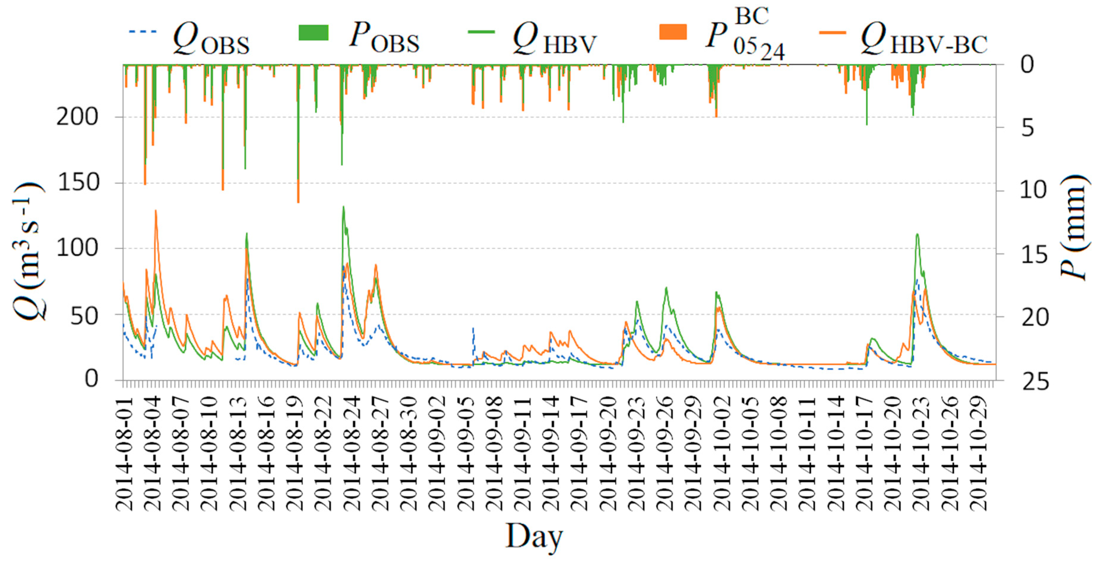
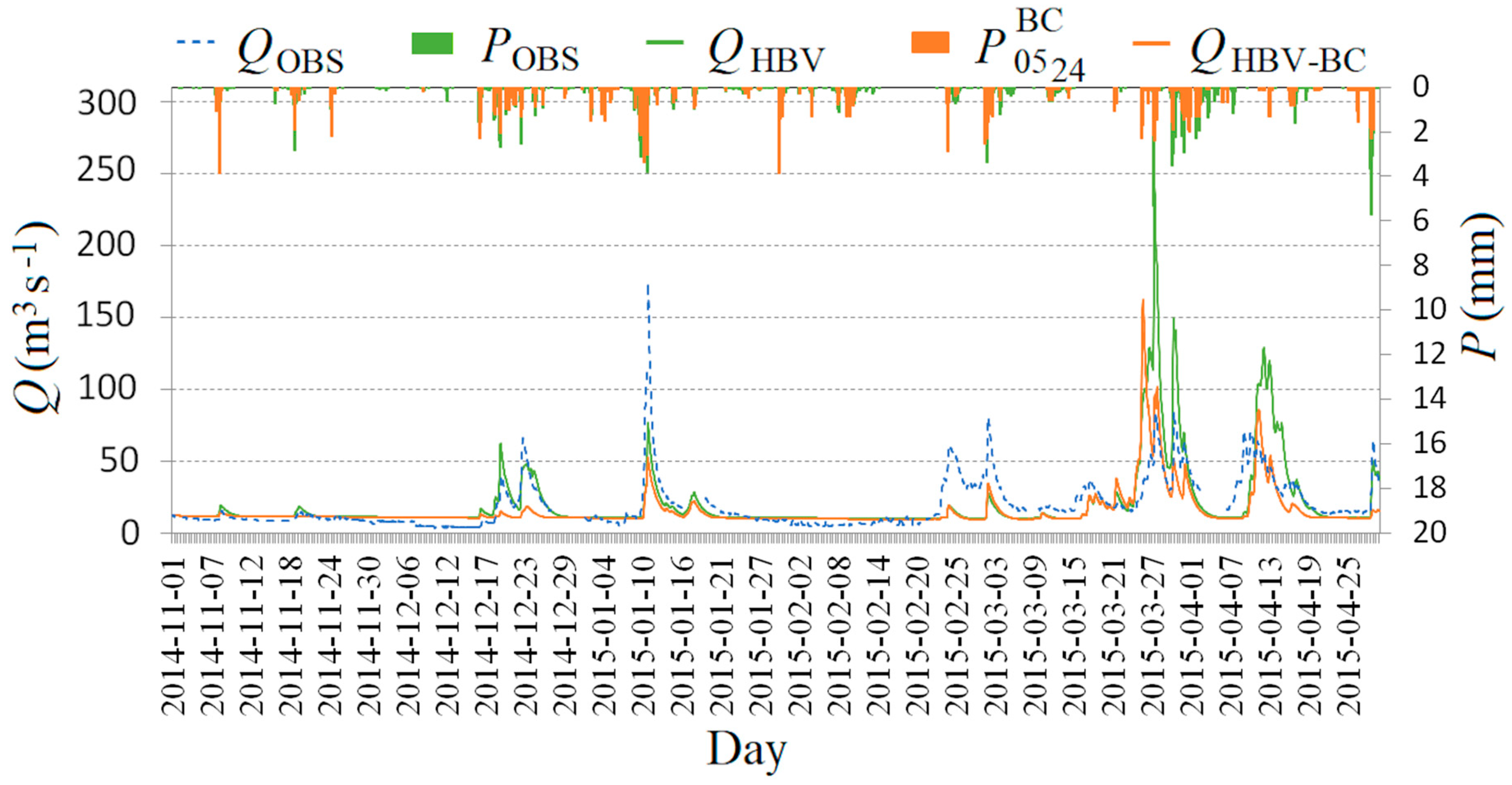
4.3.1. Simulating Discharge with Bias-Corrected Satellite Precipitation without Assimilation

In the first step of the analysis, the effects of the corrected satellite precipitation ($P_{{05}_{24}}^{\mathrm{BC}})$ on the accuracy of the HBV model simulation in summer (Figure 4) and winter (Figure 5) were examined.

Observed flow $(Q_{\mathrm{OBS}})$ was compared with the HBV simulation $\left(Q_{\mathrm{HBV}}\right)$ (first input option from the top in Figure 2) and HBV simulation with $P_{{05}_{24}}^{\mathrm{BC}}$ ($Q_{\mathrm{HBV}-\mathrm{BC}}$) (second input option from the top in Figure 2). In both seasons, a slight increase in the efficiency of the HBV model, using satellite precipitation as forcing data, $Q_{\mathrm{HBV}-\mathrm{BC}}$ (Table 3), was observed. In the summer, the $P_{{05}_{24}}^{\mathrm{BC}}$ improved the model $\mathrm{EI}$ from −0.045 to 0.103 and from −0.185 to 0.195 in the winter compared to $Q_{\mathrm{HBV}}$. Furthermore, the highest quantitative and qualitative discrepancy between observed and satellite precipitation was registered in August, which was associated with convective instability in the atmosphere. Differences in the quantitative estimation of precipitation affected the discrepancy between the $Q_{\mathrm{HBV}}$ and $Q_{\mathrm{HBV}-\mathrm{BC}}$. A noticeable improvement in the model simulation using satellite precipitation was observed in the second half of September and October.

In winter, with negative air temperatures and snow cover, quantitative information on the precipitation indirectly influenced the simulation. The main determinant of runoff is groundwater sources, however, when the snowpack disappears and the thawing of topsoil layers begins, surface and sub-surface runoff also play a major role. Therefore, at the end of the winter season during the rainy spring flood, an increase in the accuracy of the simulated hydrographs was seen, due to the impact of the corrected satellite precipitation.

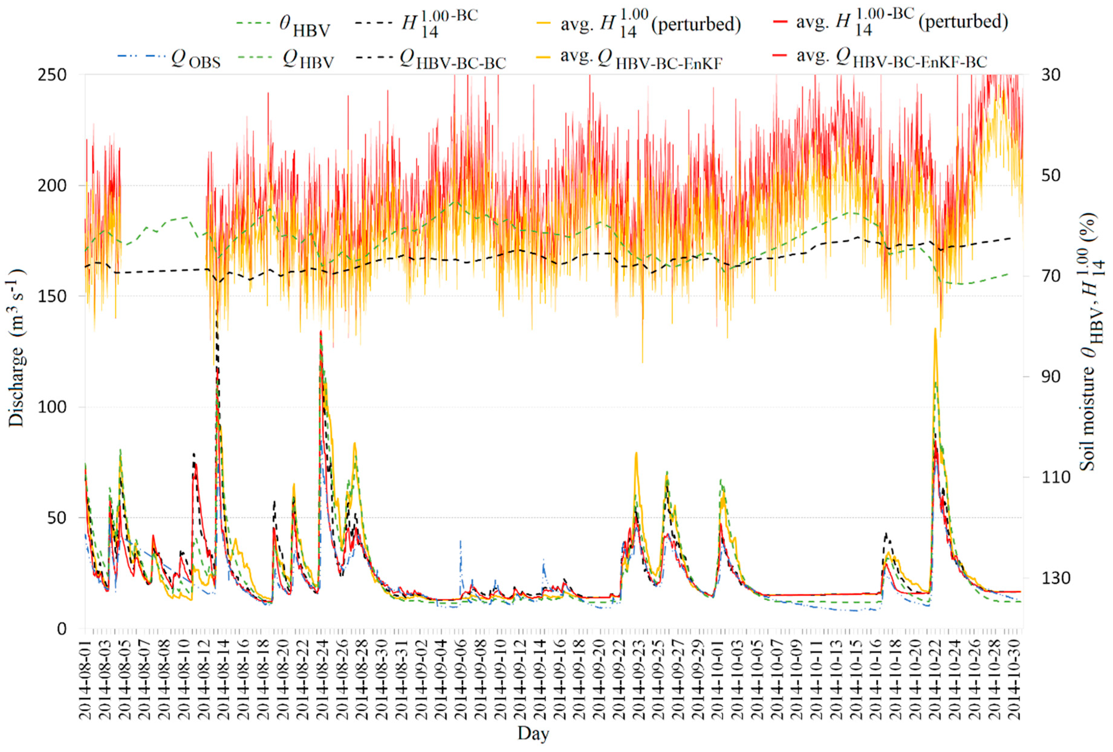
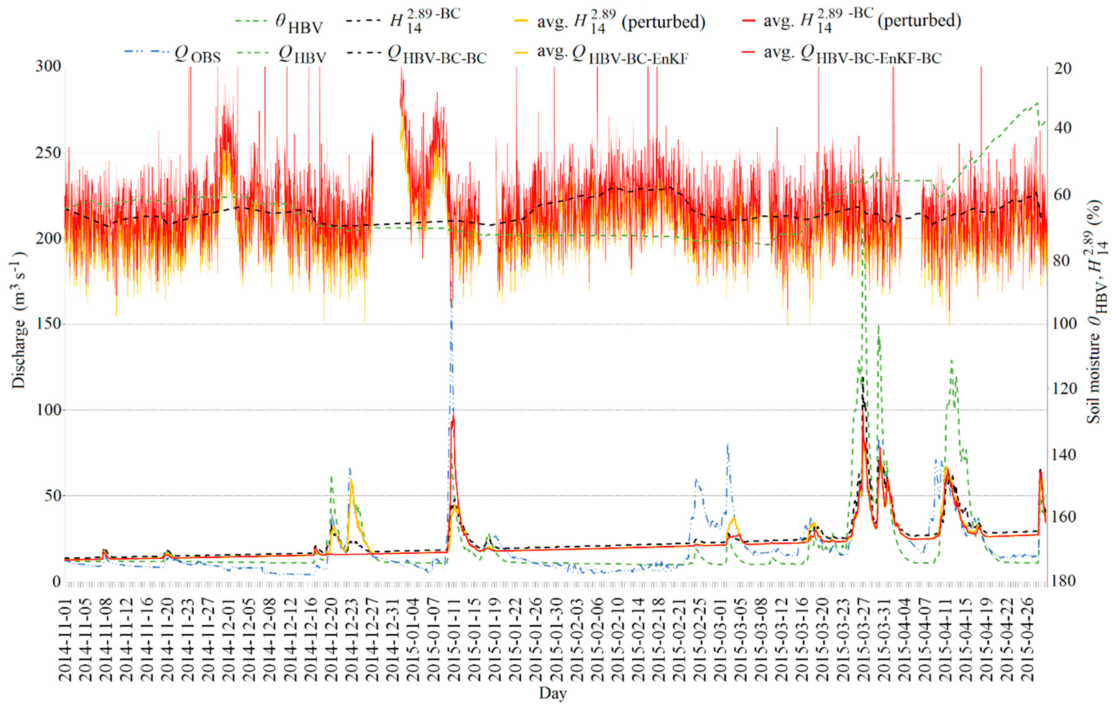
4.3.2. Simulating Discharge Using Two Methods, with Bias-Corrected Satellite Soil Moisture or with the Assimilation Procedure

The best satellite precipitation product for modeling $P_{\mathrm{OBS}}$ was $P_{{05}_{24}}^{\mathrm{BC}}$, and therefore $P_{{05}_{24}}^{\mathrm{BC}}$ was used in further analyses. The impact of the assimilation of these observations of soil moisture ($H_{14}^{1.00}$ and $H_{14}^{2.89}$) (fifth input option from top in Figure 2) in improving the accuracy of the HBV simulation using EnKF-BC as an averaged ensemble, avg. Q_{HBV-BC-EnKF-BC} (solid red line in Figure 6 and Figure 7) was determined, with results provided in Table 3. Model simulations using the assimilation procedure were compared to the assimilation of soil moisture ($H_{14}^{1.00}$ and $H_{14}^{2.89}$) (fourth input option from top in Figure 2) using EnKF, avg. $Q_{\mathrm{HBV}-\mathrm{BC}-\mathrm{EnKF}}$ (solid orange line), to the simulation using only BC satellite soil moisture as an input to the HBV model, $Q_{\mathrm{HBV}-\mathrm{BC}-\mathrm{BC}}$ (dashed black line) (third input option from top in Figure 2), as well as to the HBV simulations with observed precipitation, $Q_{\mathrm{HBV}}$ (dashed green line) (first input option from top in Figure 2). The calculations were made separately for the two satellite soil moisture products and the summer and winter seasons (left and right parts of Table 3, respectively). The upper part of Figure 6 and Figure 7 compares the soil moisture graphs (generated by the HBV model), θ_HBV (dashed green line), the unperturbed satellite observations with removed bias, $H_{14}^{\mathrm{BC}}$ (dashed black line), the averaged value of perturbed satellite observations without bias correction, avg. H₁₄ (perturbed) (solid orange line), and the averaged value of bias-free perturbed satellite soil moisture, avg. $H_{14}^{\mathrm{BC}}$ (perturbed) (solid red line).

In summer, the best overall simulation model for the period of 06:00H, 1 August 2014 to 23:00H, 31 October 2014, was the HBV model using the $P_{{05}_{24}}^{\mathrm{BC}}$ precipitation product with EnKF-BC assimilation of the $H_{14}^{1.00}$, avg. $Q_{\mathrm{HBV}-\mathrm{BC}-\mathrm{EnKF}-\mathrm{BC}}$. As soil moisture dynamics are complex, only the effects of soil moisture on runoff generation at the basin scale were modeled using the HBV. This was based on a modification of the Bucket Theory, which assumes a statistical distribution of storage capacities in a basin [43]. The rate of evaporation depends on the potential evaporation and soil water content, and similarly, the rate of percolation depends upon rain intensity and soil water content. This implies that the rate of contribution of runoff depends on soil moisture, which is a main part of the model. The largest runoff was attained in the HBV model when all the boxes were full and contributed to the runoff volume. In this case, the routine’s equations lead to maximum soil moisture storage. Precise estimation of this physical quantity (assimilation of the satellite soil moisture observation) greatly affected the simulation of flow during floods.

A good example was the summer floods which occurred from 19:00H on 22 September to 11:00H on 4 October, and from the 23:00H on 21 October to 08:00H on 26 October (Figure 6). The state variable of the assimilated satellite soil moisture $\left(H_{14}^{1.00}\right)$ served as an observation affecting the value of the runoff coefficient.

Moreover, the error in estimating the largest observed flows, in the second part of the summer season, was reduced by using the HBV model with the EnKF-BC (avg. $Q_{\mathrm{HBV}-\mathrm{BC}-\mathrm{EnKF}-\mathrm{BC}}$), resulting in a closer match between the simulated hydrograph and observed values in the last step of the simulation. Such situations were important in the process of estimating a set of initial variables at run-up when using the HBV model in forecasting mode. Of course, too high of an estimation of soil moisture resulted in an overestimation of the flow, which was visible in the period from 12:00H, 11 August to 02:00H, 26 August 2014.

In the summer, the EnKF-BC clearly impacts the simulation of hydrographs compared to the EnKF method, i.e., avg. $Q_{\mathrm{HBV}-\mathrm{BC}-\mathrm{EnKF}-\mathrm{BC}}$ (${\mathrm{R}}_0\mathrm{M}=1.140$, $\mathrm{RMSE}=6.775$ m³s⁻¹, $\mathrm{EI}=0.658$) vs. avg. $Q_{\mathrm{HBV}-\mathrm{BC}-\mathrm{EnKF}}$ (${\mathrm{R}}_0\mathrm{M}=1.192$, $\mathrm{RMSE}=8.575$ m³s⁻¹, $\mathrm{EI}=0.418$). Correction of the ensemble perturbation bias within the EnKF-BC filter reduced soil moisture values in the HBV model, and thus reduced the outflow, especially during convective precipitation, e.g., comparison of hydrographs avg. $Q_{\mathrm{HBV}-\mathrm{BC}-\mathrm{EnKF}-\mathrm{BC}}$ (solid red line) vs., $Q_{\mathrm{HBV}-\mathrm{BC}-\mathrm{EnKF}}$ (orange solid line) from 12:00H, 25 August 2014 to 29 August 2019, or from 19:00H, 22 September 2014 to 11:00H, 4 October 2014.

In summer, the positive impact of the correction and assimilation of the satellite products can be seen in the increased accuracy of the simulated hydrographs. However, in winter (i.e., from 06:00H, 1 November 2014 to 23:00H, 30 April 2015), the Sola Catchment was covered with snow, and air temperatures were negative, thereby deteriorating the quality of the $H_{14}^{1.00}$ and $H_{14}^{2.89}$ satellite products.

This resulted in an increase in the $\mathrm{RMSE}$ and a decrease in the $\mathrm{EI}$ when compared to the simulations generated by the HBV model in the summer (Table 3). In winter, the best simulation result was obtained by the assimilation of $H_{14}^{2.89}$, avg. $Q_{\mathrm{HBV}-\mathrm{BC}-\mathrm{EnKF}-\mathrm{BC}}$ (${\mathrm{R}}_0\mathrm{M}=1.139$, $\mathrm{RMSE}$ $=11.392$ ${\mathrm{m}}^3{\mathrm{s}}^{-1}$ and $\mathrm{EI}=0.567$), which proved to be more accurate than the HBV model for $H_{14}^{2.89}$ without the assimilation procedure, $Q_{\mathrm{HBV}-\mathrm{BC}-\mathrm{BC}}$ (Table 3).

The quality of the soil moisture estimation from ASCAT is poor when there is snow cover. The H₁₄/SM-DAS-2, as an ECMWF product, is validated against ground soil moisture measurement from in situ data (SSM), among others, with a single station in Poland located in the lowland [66]. The comparison between the observed data (SSM) and the H₁₄ product uses the following statistical scores: Mean bias, standard deviation, correlation coefficient and root mean square difference. A low correlation coefficient was found in Poland (0.61). Therefore, for this station, the winter and late summer data are filtered when temperatures are below +3 °C.

There were five hydrographs produced for winter river flow (Figure 7):

(i)

$Q_{\mathrm{OBS}}$, observed flow;

(ii)

$Q_{\mathrm{HBV}}$, flow simulated by HBV with $P_{\mathrm{OBS}}$ precipitation;

(iii)

$Q_{\mathrm{HBV}-\mathrm{BC}-\mathrm{BC}}$, flow simulated by HBV with $P_{{05}_{24}}^{\mathrm{BC}}$ and $H_{14}^{2.89-\mathrm{BC}}$;

(iv)

Avg. $Q_{\mathrm{HBV}-\mathrm{BC}-\mathrm{EnKF}}$ and using $P_{{05}_{24}}^{\mathrm{BC}}$ and assimilating $H_{14}^{2.89}$,

(v)

And avg. $Q_{\mathrm{HBV}-\mathrm{BC}-\mathrm{EnKF}-\mathrm{BC}}$ using $P_{{05}_{24}}^{\mathrm{BC}}$ and assimilating $H_{14}^{2.89}$ with the creation of an unbiased ensemble of model states.

Figure 7 shows that from November to mid-March, all simulated hydrographs underestimated $Q_{\mathrm{OBS}}$, yet overestimated the flood event in April. Pre-processing with the assimilation procedure more effectively estimated the flood in March and April of 2015 when compared to $Q_{\mathrm{HBV}}$, as shown by the large discrepancy between the dashed blue line with double dots ($Q_{\mathrm{OBS}}$), dashed green line ($Q_{\mathrm{HBV}}$) and solid red line (avg. $Q_{\mathrm{HBV}-\mathrm{BC}-\mathrm{EnKF}-\mathrm{BC}}$) in Figure 7. After the disappearance of the permanent snow cover at the end of March and into April, the positive impact of the satellite precipitation product, i.e., $P_{{05}_{24}}^{\mathrm{BC}},$ was evident. There was a slight difference in the March and April hydrographs between $Q_{\mathrm{HBV}-\mathrm{BC}}$ (Figure 5), $Q_{\mathrm{HBV}-\mathrm{BC}-\mathrm{BC}}$, avg. $Q_{\mathrm{HBV}-\mathrm{BC}-\mathrm{EnKF}}$ and avg. $Q_{\mathrm{HBV}-\mathrm{BC}-\mathrm{EnKF}-\mathrm{BC}}$ (Figure 7). The influence of the satellite soil moisture and its correction and assimilation was visible only to a small extent, i.e., avg. $Q_{\mathrm{HBV}-\mathrm{BC}-\mathrm{EnKF}-\mathrm{BC}}$ (${\mathrm{R}}_0\mathrm{M}=1.139$, $\mathrm{RMSE}$ $=11.392$ ${\mathrm{m}}^3{\mathrm{s}}^{-1}$ and $\mathrm{EI}=0.567$) vs. avg. $Q_{\mathrm{HBV}-\mathrm{BC}-\mathrm{EnKF}}$ (${\mathrm{R}}_0\mathrm{M}=1.160$, $\mathrm{RMSE}$ $=11.882$ ${\mathrm{m}}^3{\mathrm{s}}^{-1}$ and $\mathrm{EI}=0.551$) vs. $Q_{\mathrm{HBV}-\mathrm{BC}-\mathrm{BC}}$ (${\mathrm{R}}_0\mathrm{M}=1.161$, $\mathrm{RMSE}$ $=11.884$ ${\mathrm{m}}^3{\mathrm{s}}^{-1}$ and $\mathrm{EI}=0.529$).

In Figure 7, the negative influences of the DA procedure on the outflow from the lower linear reservoir can be seen. There is a clear increasing trend in discharge. In the HBV model, the runoff generation routine was the response function that transformed excess water from the soil moisture zone into the runoff. The water from the soil moisture zone was added to the upper box and percolated towards the lower box, representing the groundwater storage of the catchment contributing to the base flow. With a high yield from the soil, percolation was not sufficient to keep the upper reservoir empty. The generated discharge contributes directly to the upper reservoir, which represents drainage through more superficial channels. The lower reservoir, on the other hand, represents the groundwater storage of the catchment, contributing to rises in base flow. The consequence is a constant trend of flow in Figure 7. In order to optimize (decrease) the base flow, especially in the winter season (Figure 7), the procedure would likely need to be extended to interactively update past and present model states (e.g., content of upper and lower boxes in the response routine) to improve model initial conditions, and hence flow forecasts.

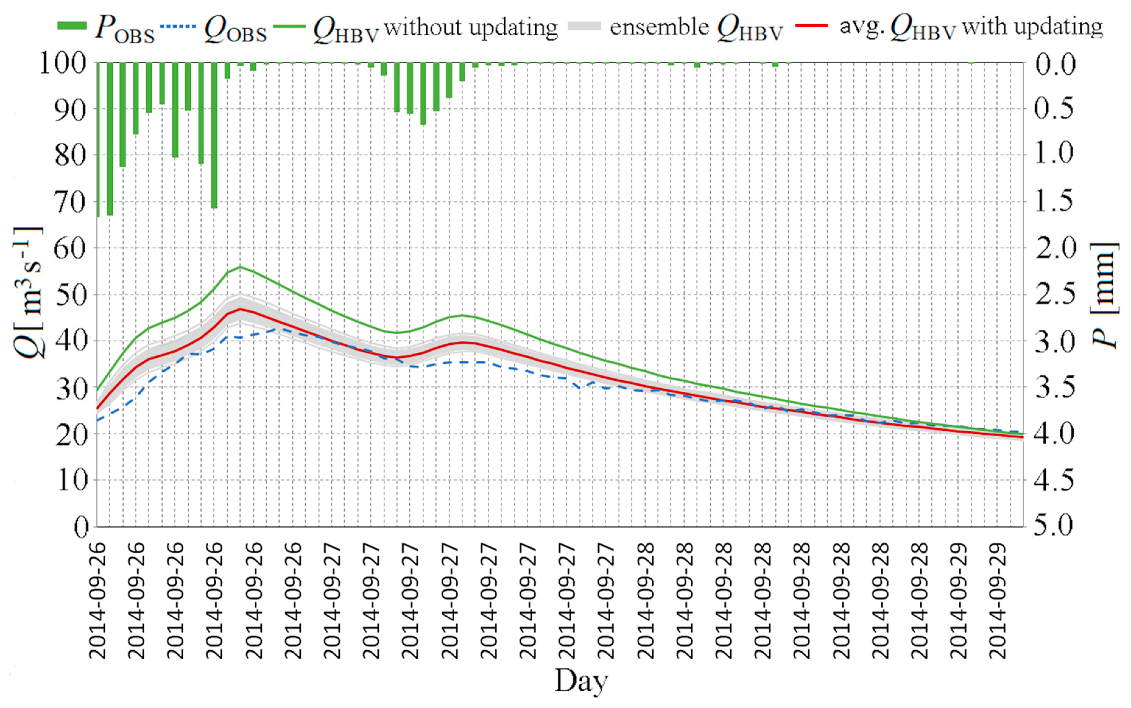
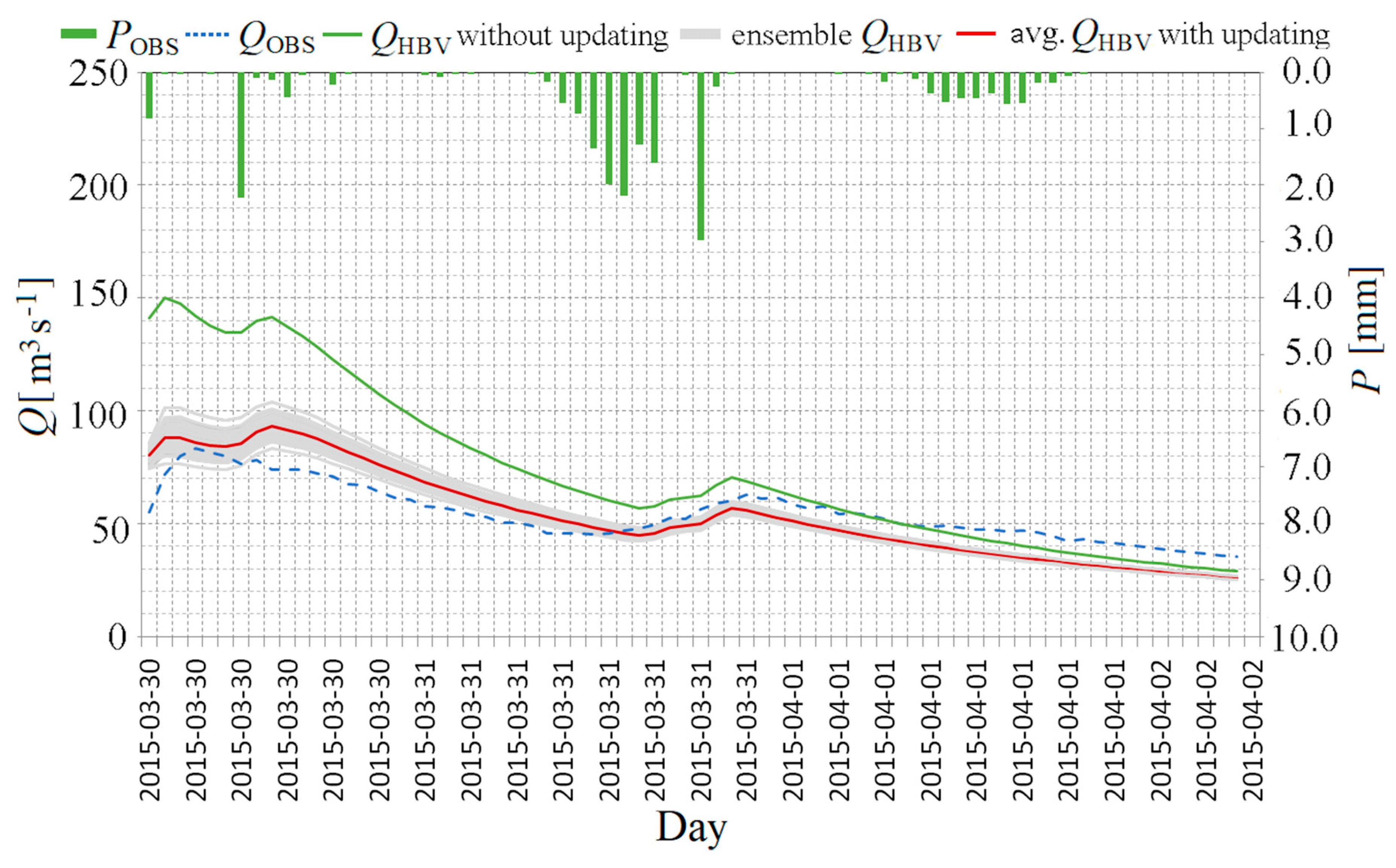
4.3.3. Examples of Hydrological Updating the HBV Model Using EnKF-BC and Simulation of the HBV Model in Forecast Mode for the Sola Basin at Zywiec for Selected Flood Events

The last element of the study evaluated the possibility of using satellite products to update hydrological forecasts and to compare forecasts carried out with and without updating between summer and winter. One flood event occurring in each of the summer and winter periods was selected. The HBV model was run in forecast mode in the last step of the updating procedure. The input to the forecast was generated using the hindcast method. For the events examined, the same length of updating (120 h) and window forecast (72 h) were used. The updated input consisted of the corrected satellite precipitation, $P_{{05}_{24}}^{\mathrm{BC}}$ and assimilation $H_{14}^{1.00}$ for summer, and $H_{14}^{2.89}$ for winter events using the EnKF-BC (according to the assessment of the accuracy of the HBV model shown in Table 3; fifth input option from the top in Figure 2). The forecasted input consisted of the observed precipitation, $P_{\mathrm{OBS}}$ (hindcast method), and the HBV model was run without the assimilation procedure (first input option from the top in Figure 2). The results showed that forecasts preceded by updating achieved better values of ${\mathrm{R}}_0\mathrm{M}$, $\mathrm{RMSE}$ and $\mathrm{EI}$ than the forecasts without updating (Table 4).

The performances of the simulations in forecast mode are shown in Figure 8 (summer) and 9 (winter). For each flooding event, three hydrographs were compared:

(i)

$Q_{\mathrm{OBS}}$—observed hydrograph (dotted blue line);

(ii)

$Q_{\mathrm{HBV}}$—forecasted hydrograph without updating (solid green line);

(iii)

and avg. $Q_{\mathrm{HBV}}$—averaged forecasted hydrograph with updating (solid red line) with the ensemble hydrographs (solid gray lines).

The flood event occurring between 06:00H on 26 September 2014 and 06:00H on 29 September 2014 is an example of a good simulation in forecasting mode. The success is likely due to the effective updating using the EnKF-BC method, which is highlighted by the difference in starting positions on the observed hydrograph (dotted blue line), the averaged hydrograph with updating by the EnKF-BC (solid red line), and the hydrograph without updating (solid green line). In this case, a large part of the forecast horizon was within the ensemble forecast (gray lines) (Figure 8). The recession in the second part of the hydrograph was smaller than that of the forecast without updating, and the forecast error in the last step of the horizon was comparable.

For the winter updating and forecasting process, two key observed quantitative parameters tied to the forecasted runoff were not available. These included the surface distribution of snow cover and the snow water equivalent. Information about these parameters was only contained within state variables that were recalculated using the snow model that was implemented in a subroutine of the HBV model. Within an update, the satellite snow observations were not assimilated. The hydrological simulation in the forecasting mode of a rainy spring flood (06:00H on 30 March 2015 to 06:00H on 2 April 2015) (Figure 9) is an example of the effective use of the correction of satellite precipitation data and the assimilation of corrected soil moisture within the updating procedure. Calculations during the update of the matrix of state variables allowed for better precision when generating the ensemble forecast through the HBV model, compared to HBV simulations without updating, which is evident from the difference in starting positions between hydrographs.

5. Summary and Conclusions

The possibility of using a satellite precipitation product correction as a forcing data, and the assimilation of soil moisture data to generate ensemble forecasts within the HBV model environment, were explored in detail using four processes. These processes include: (i) Calibration of the HBV model, (ii) removal of the bias module, BC, (iii) simulation of the HBV, with or without updating, where updating the HBV was carried out using bias-corrected satellite soil moisture which replaced the proper state variable of the HBV, or by using an assimilation procedure to create an ensemble of the model states with or without unbiased errors using an EnKF or an EnKF-BC filter, and (iv) simulation of the HBV in forecast mode with an updating procedure using assimilation of the satellite observations.

The framework proposed in the study addressed the two main stages of the HBV simulation procedure, the bias correction method and the assimilation procedure, with regards to the potential application of unbiased perturbation to soil moisture state variables. The goal of this study consisted of developing a distribution-derived transformation method with a new algorithm using three theoretical distributions (i.e., generalized exponential (GE), gamma (GA) and Weibull (WE) singly, or in pairs) to generate bias-free satellite precipitation and soil moisture data. This study proposed the use of these three probability distributions with similar random properties.

The soil moisture estimates resulting from the data assimilation procedure were sensitive to observations and model error variance. The model error had an impact upon the error covariance between observations and the model state, and the effectiveness of the assimilation procedure used. This paper proposed removing bias from the ensemble of model states using a distribution-derived transformation method dynamically combined with a Kalman filter. This procedure included probability distribution fitting, validation and correction of the ensemble perturbation bias.

The deterministic hydrological model, HBV, was calibrated using historical data from 06:00H on 1 January 2008 to 06:00H on 31 July 2014, and was not re-calibrated with input data derived from satellite-based products. This study examined the impact of the proposed procedure (bias correction and assimilation using an ensemble Kalman filter, EnKF-BC) on the accuracy of the HBV-simulated hydrographs during two validation periods: (i) Summer from 06:00H, 1 August 2014 to 23:00H, 31 October 2014, and (ii) winter from 06:00H, 1 November 2014 to 06:00H, 30 April 2015. The calculations were carried out using data from the Sola Mountain Catchment in southern Poland. The HBV model was updated using two methods: Assimilation of satellite soil moisture observations, and bias correction of the satellite soil moisture products without assimilation. The proposed HBV simulation procedure used corrected satellite precipitation $P_{{05}_{24}}$ as forcing data. The results of these simulations were compared to simulations with observed precipitation and flow.

The last stage of this research presented examples using the HBV model and the data assimilation procedure, i.e., the methods for the assimilation of satellite soil moisture products for updating in short-term hydrological forecasting. The algorithms enabled the development of ensemble (interval) forecasts based on the EnKF method. Two summer and winter flooding events were analyzed via the updating of events through a procedure using data assimilation. The model’s forecasting ability was then compared to that of the model with no updating. Performance forecasts were made using simulations by the HBV model in forecasting mode using the hindcast method.

In accordance with the results, the following conclusions can be made:

• The most effective transformation function for observed daily precipitation ($P_{\mathrm{OBS}}$) was the GE distribution. For satellite precipitation ($P_{{05}_{24}}$), the WE distribution was the most effective.
• The best-suited transformation function for the HBV soil moisture (${\theta }_{\mathrm{HBV}}$) was the WE distribution in both winter and summer. For satellite soil moisture ($H_{14}^{1.00}$), the optimum transformation function was GA in both winter and summer. For $H_{14}^{2.89}$, the optimum transformation function was WE in the winter and GA in the summer.
• Removing bias from the satellite precipitation improved the modeling accuracy of $P_{\mathrm{OBS}}$, both during distribution fitting and the validation of the product. Removing the bias from satellite soil moisture products, however, was only effective in summer during distribution fitting and validation. In winter, negative efficiency index values were observed.
• The tested satellite product, $P_{{05}_{24}}^{\mathrm{BC}}$, without the assimilation soil moisture product, did not significantly improve hydrograph performance, especially in the summer. This is likely due to the influence of convective precipitation upon runoff. The quality of the spatial distribution of precipitation, however, was an important factor influencing the quality of the simulated hydrograph, especially in the mountain catchment.
• After taking into account the assimilation of the satellite soil moisture product, the best simulation model included the assimilation of $H_{14}^{1.00}$ in summer. In winter, a negligible improvement was observed between the simulated hydrograph using the corrected assimilation $H_{14}^{2.89-\mathrm{BC}}$ and the assimilation $H_{14}^{2.89}$ using EnKF and EnKF-BC filters.
• The HBV model with updating in the forecast mode generally performed poorly; however, it improved the forecast compared to the HBV without updating. It should be noted that the forecasts were calculated based on matrix state variables determined in the final step of updating using the assimilation of satellite soil moisture.

References

1. Refsgaard, J.C. Validation and Intercomparison of Different Up-dating Procedures for Real-Time Forecasting. Nord. Hydrol. 1997, 28, 65–84. [Google Scholar] [CrossRef]
2. Yang, X.; Michelle, C. Flood forecasting with a watershed model: A new method of parameter updating. Hydrol. Sci. 2001, 45, 537–547. [Google Scholar] [CrossRef]
3. Xiong, L.; O’Connor, K.M. Comparison of four updating models for real-time river flow forecasting. Hydrol. Sci. J. 2002, 47, 621–639. [Google Scholar] [CrossRef] [Green Version]
4. Wöhling, T.; Lennartz, F.; Zappa, M. Technical Note: Updating procedure for flood forecasting with conceptual HBV-type models. Hydrol. Earth Syst. Sci. 2006, 10, 783–788. [Google Scholar] [CrossRef] [Green Version]
5. Lehner, B.; Doll, P.; Alcamo, J.; Henrichs, T.; Kaspar, F. Estimating the impact of global change on flood and drought risks in Europe: A continental, integrated analysis. Clim. Chang. 2006, 75, 273–299. [Google Scholar] [CrossRef]
6. Piani, C.; Weedon, G.P.; Best, M.; Gomes, S.M.; Viterbo, P.; Hagemann, S.; Haerter, J.O. Statistical bias correction of global simulated daily precipitation and temperature for the application of hydrological models. J. Hydrol. 2010, 395, 199–215. [Google Scholar] [CrossRef]
7. Bennet, J.C.; Grose, M.R.; Post, D.A.; Ling, F.L.N.; Corney, S.P.; Bindoff, N.L. Performance of quantile-quantile bias correction for use in hydroclimatological projections. In Proceedings of the 19th International Congress on Modeling and Simulation, Perth, Australia, 12–16 December 2011; Available online: http://mssanz.org.au./modsim2011 (accessed on 30 April 2016).
8. Sharma, D.; Gupta, A.D.; Babel, M.S. Spatial disaggregation of bias-corrected GCM precipitation for improved hydrologic simulation: Ping River Basin, Thailand. Hydrol. Earth Syst. Sci. 2007, 11, 1373–1390. [Google Scholar] [CrossRef] [Green Version]
9. Müller, M.F.; Thompson, S.E. Bias adjustment of satellite rainfall data through stochastic modeling: Methods development and application to Nepal. Adv. Water Resour. 2013, 60, 121–134. [Google Scholar] [CrossRef] [Green Version]
10. Reichle, R.H.; Koster, R.D. Bias reduction in short records of satellite soil moisture. Geophys. Res. Lett. 2004, 31, L19501. [Google Scholar] [CrossRef]
11. Alvarez-Garreton, C.; Ryu, D.; Western, A.W.; Crow, W.T.; Robertson, D.E. The impacts of assimilating satellite soil moisture into a rainfall-runoff model in a semi-arid catchment. J. Hydrol. 2014, 519, 2763–2774. [Google Scholar] [CrossRef]
12. Kalman, R.E. A new approach to linear filtering and prediction problems. J. Basic Eng. 1960, 82, 35–45. [Google Scholar] [CrossRef]
13. Xie, X.; Zhang, D. Data assimilation for distributed hydrological catchment modeling via ensemble Kalman filter. Adv. Water Resour. 2010, 33, 678–690. [Google Scholar] [CrossRef]
14. Xiong, J.; Huang, X.L.; Cao, Z.Y. Assimilating observation data into hydrological model with ensemble Kalman filter. Adv. Mater. Res. 2011, 255, 3632–3636. [Google Scholar] [CrossRef]
15. Samuel, J.; Coulibaly, P.; Dumedah, G.; Moradkhani, H. Assessing model state and forecasts variation in hydrologic assimilation. J. Hydrol. 2014, 513, 127–141. [Google Scholar] [CrossRef]
16. Rasmussen, J.; Madsen, H.; Jensen, K.H.; Refsgaard, J.C. Data assimilation in integrated hydrological modeling using ensemble Kalman filtering: Evaluating the effect of ensemble size and localization on filter performance. Hydrol. Earth Syst. Sci. 2015, 19, 2999–3013. [Google Scholar] [CrossRef]
17. Thiboult, A.; Anctil, F. On the difficulty to optimally implement the Ensemble Kalman filter; An experiment based on many hydrological models and catchments. J. Hydrol. 2015, 529, 1147–1160. [Google Scholar] [CrossRef]
18. Clark, M.P.; Rupp, D.E.; Woods, R.A.; Zheng, X.; Ibbitt, R.P.; Slater, A.G.; Schmidt, J.; Uddstrom, M.J. Hydrologic data assimilation with the ensemble Kalman filter: Use of stream-flow observations to update states in a distributed hydrological model. Adv. Water Resour. 2008, 31, 1309–1324. [Google Scholar] [CrossRef]
19. Reynolds, S.G. The gravimetric method of soil moisture determination. Part I. A study of equipment and methodological problem. J. Hydrol. 1970, 11, 258–273. [Google Scholar] [CrossRef]
20. Zheng, W.; Zhan, X.; Liu, J.; Ek, M. A Preliminary Assessment of the Impact of Assimulating Satellite Soil Moisture Data Products on NCEP Global Forecast System. Adv. Meteorol. 2018, 2018, 7363194. [Google Scholar] [CrossRef]
21. Zhan, W.; Pan, M.; Wanders, N.; Wood, E.F. Correction of real-time satellite precipitation with satellite soil moisture observations. Hydrogeol. Earth Syst. Sci. 2015, 19, 4275–4291. [Google Scholar] [CrossRef] [Green Version]
22. Reichle, R.H.; Walker, J.P.; Koster, R.D.; Houser, P.R. Extended versus ensemble Kalman filtering for land data assimilation. J. Hydrometeorol. 2002, 3, 728–740. [Google Scholar] [CrossRef]
23. Crow, W.T.; Ryu, D. A new data assimilation approach for improving runoff prediction using remotely-sensed soil moisture retrievals. Hydrol. Earth Syst. Sci. 2009, 13, 1–16. [Google Scholar] [CrossRef] [Green Version]
24. Brocca, L.; Melon, F.; Moramarco, T.; Wagner, W.; Naeimi, V.; Bartalis, Z.; Hasenauer, S. Improving runoff prediction through the assimilation of the ASCAT soil moisture product. Hydrol. Earth Syst. Sci. 2010, 14, 1881–1893. [Google Scholar] [CrossRef] [Green Version]
25. Corato, G.; Matgen, P.; Fenicia, F.; Schlaffer, S.; Chini, M. Assimilating satellite-derived soil moisture products into a distributed hydrological model. In Proceedings of the International Geoscience and Remote Sensing Symposium (IGARSS), Quebec City, QC, Canada, 13–18 July 2014; pp. 3315–3318. [Google Scholar] [CrossRef]
26. Hirpa, F.A.; Gebremichael, M.; Hopson, T.M.; Wojick, R.; Lee, H. Assimilation of Satellite Soil Moisture Retrievals into a Hydrologic Model for Improving River Discharge. Remote Sens. Terr. Water Cycle 2014, 206, 319–329. [Google Scholar] [CrossRef]
27. Massari, C.; Brocca, L.; Tarpanelli, A.; Moramarco, T. Data assimilation of satellite soil moisture into rainfall-runoff modeling: A complex recipe? Remote Sens. 2015, 7, 11403–11433. [Google Scholar] [CrossRef]
28. Alvarez-Garreton, C.; Ryu, D.; Western, A.W.; Crow, W.T.; Su, C.-H.; Robertson, D.R. Dual assimilation of satellite soil moisture to improve streamflow prediction in data-scarce catchments. Water Resour. Res. 2016, 52, 5357–5375. [Google Scholar] [CrossRef] [Green Version]
29. Chen, H.; Yang, D.; Liu, Y.; Zhang, B. Data assimilation techniques based on ensemble Kalman filter for improving soil water content estimation. Trans. Chin. Soc. Agric. Eng. 2016, 32, 99–104. [Google Scholar] [CrossRef]
30. Liu, Y.; Wang, W.; Hu, Y. Investigating the impact of surface soil moisture assimilation on state and parameter estimation in SWAT model based on the ensemble Kalman filter in upper Huai River basin. J. Hydrol. Hydromech. 2017, 65, 123–133. [Google Scholar] [CrossRef] [Green Version]
31. Xu, X.; Tolson, B.A.; Li, J.; Davison, B. Assimilation of Synthetic Remotely Sensed Soil Moisture in Environment Canada’s MESH Model. IEEE J. Sel. Top. Appl. Earth Obs. Remote Sens. 2017, 10, 1317–1327. [Google Scholar] [CrossRef]
32. Laiolo, P.; Gabellani, S.; Campo, L.; Cenci, L.; Silvestro, F.; Delogu, F.; Boni, G.; Rudari, R.; Puca, S.; Pisani, A.R. Assimilation of remote sensing observations into a continuous distributed hydrological model: Impacts on the hydrologic cycle. In Proceedings of the IEEE International Geoscience and Remote Sensing Symposium, Milan, Italy, 26–31 July 2015; pp. 1308–1311. [Google Scholar] [CrossRef]
33. Alvarez-Garreton, C.; Ryu, D.; Western, A.W.; Su, C.H.; Crow, W.T.; Robertson, D.E.; Leahy, C. Improving operational flood ensemble prediction by the assimilation of satellite soil moisture: Comparison between lumped and semi-distributed schemes. Hydrol. Earth Syst. Sci. 2015, 19, 1659–1676. [Google Scholar] [CrossRef]
34. Ryu, D.; Crow, W.T.; Zhan, X.; Jackson, T.J. Correcting Unintended Perturbation Biases in Hydrologic Data Assimilation. J. Hydrometeorol. 2009, 10, 734–750. [Google Scholar] [CrossRef]
35. Baguis, P.; Roulin, E. Soil Moisture Data Assimilation in a Hydrological Model: A Case Study in Belgium Using Large-Scale Satellite Data. Remote Sens. 2017, 10, 820. [Google Scholar] [CrossRef]
36. Cannon, A.J. Probabilistic multisite precipitation downscaling by an expanded Bernoulli-Gamma density network. J. Hydrometeorol. 2008, 9, 1284–1300. [Google Scholar] [CrossRef]
37. Lipski, C.; Kostuch, R.; Ryczek, M. Hydrological characteristics of the upper part of the Sola river basin against the background of physographical conditions, climate and use. Monogr. Tech. Comm. Rural Infrastruct. PAN 2005, 2, 75–82. [Google Scholar]
38. European Organisation for the Exploitation of Meteorological Satellites (EUMETSAT). Product User Manual (PUM) for Product H05-PR-OBS-5A; Accumulated Precipitation at Ground by Blended MW and IR. EUMETSAT Satellite Application Facility on Support to Operational Hydrology and Water Management. Doc.No: SAF/HSAF/PUM-05A, Revision 1.3.; EUMETSAT: Darmstadt, Germany, 2015; Available online: http://hsaf.meteoam.it/documents/PUM/SAF_HSAF_PUM-05A_1_3.pdf (accessed on 30 May 2016).
39. European Organisation for the Exploitation of Meteorological Satellites (EUMETSAT). Product User Manual (PUM) for Product H14-SM-DAS-2; Soil Moisture Profile Index in the Roots Region by Scatterometer Data Assimilation. EUMETSAT Satellite Application Facility on Support to Operational Hydrology and Water Management. Doc.No: SAF/HSAF/PUM-14, Revision 1.1.; EUMETSAT: Darmstadt, Germany, 2015; Available online: http://hsaf.meteoam.it/documents/PUM/SAF_HSAF_PUM-14_1_1.pdf (accessed on 30 May 2016).
40. Bergström, S. Development and Application of a Conceptual Runoff Model for Scandinavian Catchments; Bulletin Series A; Lund Institute of Technology, University of Lund: Lund, Sweden, 1976; Volume 52, p. 134. [Google Scholar]
41. Bergström, S. The HBV Model: Its Structure and Applications; Swedish Meteorological and Hydrological Institute: Norrköping, Sweden, 1992; p. 35. [Google Scholar]
42. Bergström, S. The HBV model. In Computer Models of Watershed Hydrology; Singh, V., Ed.; Water Resource Publishing: Highlands Ranch, CO, USA, 1995; pp. 443–476. [Google Scholar]
43. Lindström, G.; Johansson, B.; Persson, M.; Gardelin, M.; Bergström, S. Development and test of the distributed HBV-96 hydrological model. J. Hydrol. 1997, 201, 272–288. [Google Scholar] [CrossRef]
44. Seibert, J.; Vis, M.J.P. Teaching hydrological modeling with a user-friendly catchment-runoff-model software package. Hydrol. Earth Syst. Sci. 2012, 16, 3315–3325. [Google Scholar] [CrossRef] [Green Version]
45. Brassel, K.E.; Reif, D. A Procedure to Generate Thiessen Polygons. Geogr. Anal. 2010, 1, 289–303. [Google Scholar] [CrossRef]
46. Wilby, R.L.; Hassan, H.; Hanaki, K. Statistical downscaling of hydrometeorological variables using general circulation model output. J. Hydrol. 1998, 205, 1–19. [Google Scholar] [CrossRef]
47. Sequí, P.Q.; Ribes, A.; Martin, E.; Habets, F.; Boé, J. Comparison of three downscaling methods in simulating the impact of climate change on the hydrology of Mediterranean basins. J. Hydrol. 2010, 383, 111–124. [Google Scholar] [CrossRef] [Green Version]
48. Ahmed, K.F.; Wang, G.; Silander, J.; Wilson, A.M.; Allen, J.M.; Horton, R.; Anyah, R. Statistical downscaling and bias correction of climate model outputs for climate change impact assessment in the U.S. northeast. Glob. Planet. Chang. 2013, 100, 320–332. [Google Scholar] [CrossRef] [Green Version]
49. Gudmundsson, J.B.; Bremnes, J.E.; Haugen, J.E.; Engen-Skaugen, T. Technical Note: Downscaling RCM precipitation to the station scale using statistical transformations—A comparison of methods. Hydrol. Earth Syst. Sci. 2012, 16, 3383–3390. [Google Scholar] [CrossRef]
50. Maraun, D. Bias Correction, Quantile Mapping, and Downscaling: Revisiting the Inflation Issue. J. Clim. 2013, 26, 2137–2143. [Google Scholar] [CrossRef] [Green Version]
51. Rojas, R.; Feyen, L.; Dosio, A.; Bavera, D. Improving pan-European hydrological simulation of extreme events through statistical bias correction of RCM-driven climate simulation. Hydrol. Earth Syst. Sci. 2011, 15, 2599–2620. [Google Scholar] [CrossRef]
52. Wood, A.W.; Leung, L.R.; Sridhar, V.; Lettenmaier, D.P. Hydrologic Implications of Dynamical and Statistical Approaches to Downscaling Climate Model Outputs. Clim. Chang. 2004, 62, 189–216. [Google Scholar] [CrossRef]
53. Salvi, K.; Kannan, S.; Ghosh, S. Statistical Downscaling and Bias Correction for Projections of Indian Rainfall and Temperature in Climate Change Studies. In International Conference on Environmental and Computer Science IPCBEE; IACSIT Press: Singapore, 2011; Volume 19, pp. 7–11. Available online: http://www.ipcbee.com/vol19/2-ICECS2011R00006.pdf (accessed on 30 April 2016).
54. Cannon, A.J. Neural networks for probabilistic environmental prediction: Conditional Density Estimation Network Creation and Evaluation (CaDENCE) in R. Comput. Geosci. 2012, 41, 126–135. [Google Scholar] [CrossRef]
55. Kurnik, B.; Kajfe§-Bogataj, L.; Ceglar, A. Correcting mean and extremes in monthly precipitation from 8 regional climate models over Europe. Clim. Past Discuss. 2012, 8, 953–986. [Google Scholar] [CrossRef] [Green Version]
56. Welch, G.; Bishop, G. An Introduction to the Kalman Filter; Technical Report for University of North Carolina at Chapel Hill: Chapel Hill, NC, USA, 2006. [Google Scholar]
57. Evensen, G. The Ensemble Kalman Filter. Theoretical formulation and practical implementation. Ocean. Dyn. 2003, 53, 343–367. [Google Scholar] [CrossRef]
58. Whitaker, J.S.; Hamill, T.M. Ensemble Data Assimilation without Perturbed Observations. AMS Am. Meteorol. Soc. 2002, 130, 1913–1924. [Google Scholar] [CrossRef]
59. McMillan, H.; Jackson, B.; Clark, M.; Kavetski, D.; Woods, R. Rainfall uncertainty in hydrological modeling: An evaluation of multiplicative error models. J. Hydrol. 2011, 400, 83–94. [Google Scholar] [CrossRef]
60. Johnson, N.L.; Kotz, S.; Balakrishnan, N. Continuous Univariate Distributions; Wiley Series in Probability and Statistics; Wiley-Interscience: Cambridge, UK, 1994; p. 761. [Google Scholar]
61. Akaike, H. A new look at the statistical model identification. IEEE Trans. Autom. Control. Ac. 1974, 19, 716–722. [Google Scholar] [CrossRef]
62. Friedrich, J.O.; Adhikari, N.K.J.; Beyene, J. The ratio of means method as an alternative to mean differences for analyzing continuous outcome variables in meta-analysis: A simulation study. BMC Med. Res. Methodol. 2008, 8, 32. [Google Scholar] [CrossRef] [PubMed]
63. Chai, T.; Draxler, R.R. Root mean square error (RMSE) or mean absolute error (MAE)? Arguments against avoiding RMSE in the literature. Geosci. Model. Dev. 2014, 7, 1247–1250. [Google Scholar] [CrossRef]
64. Nash, J.E.; Sutcliffe, J.V. River flow forecasting through conceptual models, Part I—A discussion of principles. J. Hydrol. 1970, 10, 282–290. [Google Scholar] [CrossRef]
65. Houghton-Carr, H.A. Assessment criteria for simple conceptual daily rainfall-runoff models. Hydrol. Sci. J. 2009, 44, 237–261. [Google Scholar] [CrossRef]
66. EUMETSAT Satellite Application Facility on Support to Operational Hydrology and Water Management. Product User Manual (PUM) for product H14-SM-DAS-2. 2012. Available online: http://confluence.ecmwf.int/SAF-HSAF-PUM-14.pdf (accessed on 30 June 2019).
67. Gupta, R.D.; Kundu, D. Generalized exponential distributions. Aust. N. Z. J. Stat. 1999, 41, 173–188. [Google Scholar] [CrossRef]
68. Gupta, R.D.; Kundu, D. Exponentiated exponential family; an alternative to gamma and Weibull. Biom. J. 2001, 43, 117–130. [Google Scholar] [CrossRef]
Figure 1. Hydrographic map of the Sola Watershed at Zywiec, including the location of the precipitation points for P 05 24 European Organisation for the Exploitation of Meteorological Satellites (EUMETSAT) Satellite Application Facility for Support to Operational Hydrology and Water Management (H-SAF) precipitation rate at the ground, and for P OBS , and for H14 H-SAF soil moisture points.
Water 11 02138 g001
Figure 2. The block diagram of the methodology, where POBS, TOBS and QOBS represent mean ground-based precipitation, temperature and river discharge, respectively. P SAT represents the P 05 24 and H 14 , H 14 1.00 and H 14 2.89 represent soil moisture observations; Q HBV is the product of the HBV model without correction and assimilation procedures; Q HBV BC represents the product of the HBV model with bias-corrected satellite precipitation and without assimilation; Q HBV BC BC is the product of the HBV model with bias-corrected satellite precipitation and with bias-corrected satellite soil moisture data without assimilation; Q HBV BC EnKF is the product of the HBV model with bias-corrected satellite precipitation and with assimilation of the satellite soil moisture (EnKF); and Q HBV BC EnKF BC represents the product of the HBV model with bias-corrected satellite precipitation and with assimilation of the satellite soil moisture data with bias correction of the perturbed soil moisture for the creation of an unbiased ensemble of model states (EnKF-BC).
Water 11 02138 g002
Figure 3. Data assimilation algorithm for updating the Hydrologiska Byråns Vattenbalansavdelning (HBV) model (EnKF-BC). Distribution fitting of the ensemble Kalman filter with bias correction (EnKF-BC) (left part) and assimilation procedure including the EnKF-BC (right part).
Water 11 02138 g003
Figure 4. The comparison of Q OBS (observed flow; blue dotted line), Q HBV (HBV product for P OBS ; green solid line), Q HBV BC (HBV product for P 05 24 BC without assimilation; solid orange line), and P OBS (green bar), with P 05 24 BC (orange bar) in the Sola Basin at Zywiec in the summer period from 06:00H 1 August 2014 to 23:00H 31 October 2014.
Water 11 02138 g004
Figure 5. The comparison of Q OBS (observed flow; blue dotted line), Q HBV (HBV product for P OBS ; green solid line), Q HBV BC (HBV product for P 05 24 BC without assimilation; solid orange line), and P OBS (green bar), with   P 05 24 BC (orange bar) in the Sola basin at Zywiec in the winter period from 06:00H 1 November 2014 to 23:00H 30 April 2015.
Water 11 02138 g005
Figure 6. The comparison of Q OBS (observed flow; dashed blue line with double dots),   Q HBV (HBV product for P OBS ; dashed green line), Q HBV BC BC (HBV product for P 05 24 BC and for H 14 1.00 BC without assimilation; dashed black line), avg. Q HBV BC EnKF (averaged HBV product for P 05 24 BC with assimilation the H 14 1.00 using the EnKF filter; solid orange line), avg. Q HBV BC EnKF BC (averaged HBV product for P 05 24 BC with assimilation the H 14 1.00 using EnKF-BC filter; solid red line), θ HBV (HBV soil moisture product, dashed green line), H 14 1.00 BC (corrected satellite soil moisture product; dashed black line), avg.   H 14 1.00 (perturbed) (averaged ensemble of perturbed H 14 1.00 without BC method; solid orange line) with avg.   H 14 1.00 BC (perturbed) (averaged ensemble of perturbed H 14 1.00 with BC method; solid red line) in the Sola Basin at Zywiec in the summer period from 06:00H, 1 August 2014 to 23:00H, 31 October 2014.
Water 11 02138 g006
Figure 7. The comparison of Q OBS (observed flow; dashed blue line with double dots),   Q HBV (HBV product for P OBS ; dashed green line), Q HBV BC BC (HBV product for P 05 25 BC and for H 14 2.89 BC without assimilation; dashed black line), avg. Q HBV BC EnKF   (averaged HBV product for P 05 24 BC with assimilation the H 14 2.89 using EnKF filter; solid orange line) and avg. Q HBC BC EnKF BC (averaged HBV product for P 05 24 BC with assimilation the H 14 2.89 using EnKF-BC filter; solid red line), and θ HBV (HBV soil moisture product; dashed green line), H 14 2.89 BC (corrected satellite soil moisture product; dashed black line), avg.   H 14 2.89 (perturbed) (averaged ensemble of perturbed H 14 2.89 without BC method, solid orange line) with avg.   H 14 2.89 BC (perturbed) (averaged ensemble of perturbed H 14 2.89 with BC method; solid red line) in the Sola Basin at Zywiec in the winter period from 06:00H, 1 November 2014 to 23:00H, 30 April 2015.
Water 11 02138 g007
Figure 8. The comparison of Q OBS (observed flow; blue dotted line), Q HBV (HBV product without updating; solid green line), avg. Q HBV with updating (averaged HBV product; solid red line) with updating ( P 05 24 BC and assimilation of H 14 1.00 using EnKF-BC) for P OBS (green bar), and ensemble Q HBV (HBV product with updating; solid gray lines) in the Sola Basin at Zywiec, obtained for simulation of the HBV model in forecast mode in the period from 06:00H,26 September 2014 to 06:00H, 29 September 2014 (72 h).
Water 11 02138 g008
Figure 9. The comparison of Q OBS (observed flow; blue dotted line), Q HBV (HBV product without updating; solid green line), avg. Q HBV with updating (averaged HBV product; solid red line) with updating ( P 05 24 BC and assimilation of H 14 2.89 using EnKF-BC) for P OBS (green bar), and ensemble Q HBV (HBV product with updating; solid gray lines) in the Sola Basin at Zywiec, obtained for the simulation of the HBV model in forecast mode for the period from 06:00H, 30 Mach 2015 to 06:00H, 2 April 2015 (72 h).
Water 11 02138 g009