Sediment Transport in Sewage Pressure Pipes, Part I: Continuous Determination of Settling and Erosion Characteristics by In-Situ TSS Monitoring Inside a Pressure Pipe in Northern Germany

Abstract

Continuous measurement systems are widely spread in sewers, especially in non-pressure systems. Due to its relatively low costs, turbidity sensors are often used as a surrogate for other indicators (solids, heavy metals, organic compounds). However, little effort is spent to turbidity sensors in pressurized systems so far. This work presents the results of one year in-situ turbidity/total suspended solids (TSS) monitoring inside a pressure pipe (600 mm diameter) in an urban region in northern Germany. The high-resolution sensor data (5 s interval) are used for the determination of solids sedimentation (within pump pauses) and erosion behavior (within pump sequences). In-situ results from sensor measurements are similar to laboratory results presented in previous studies. TSS is decreasing exponentially in pump pauses under dry weather inflow with an average of 0.23 mg/(L s). During pump sequences, solids eroded completely at a bed shear stress of 0.5 N/m². Sedimentation and erosion behavior changes with the inflow rate. Solids settle faster with increasing inflow: at storm water inflow with an average of 0.9 mg/(L s) and at diurnal inflow variation up to 0.6 mg/(L s) at 12:00 a.m. The results are used as calibration data for a sediment transport simulation in Part II.

1. Introduction

The physical characterization of sewage is indispensable for optimization efforts in all areas of wastewater management. Pumping processes are usually necessary in sewage and storm water transport. Because of their frequent use, all related processes offer high optimization potential, to name only a few: sediment transport, energy consumption, and storm water management.

The main key to process understanding and optimization lies in data quality and quantity. Advanced optimization tools (e.g., numerical simulations) are especially data greedy. Quality and quantity varies with the data collection method: either ex-situ or in-situ. Ex-situ methods are primary laboratory experiments. Experiments simulate real world conditions as accurately as possible and subsequently transfer the results into a representative model region. For example, most stream tests try to simulate more-or-less real-life conditions.

The advantage of in-situ methods is the proximity to real life. Thus, an imitation is not required. To measure undisturbed processes, impacts on the system should be kept by a minimum.

Erosion and sedimentation of particulate matter in sewage are the dominating physical effects regarding the above-mentioned themes (sediment transport, energy consumption, storm water management). In the past, settling and erosion behavior have been determined by ex-situ experiments [1,2,3,4,5,6,7]. In case of [1,2], several laboratory experiments were conducted to describe erosion and settling behavior of the raw sewage inflow to a pumping station (PS) in an urban drainage system in Rostock (northern Germany). Consequently, the derived results are only temporal snapshots of continuous highly dynamic sewer processes. A continuous description based on permanent (in-situ) measurement allows, by far, more statements about raw sewage transport behavior. In this study, the transport behavior inside a pressure pipe is of interest. Therefore, the measurement is located directly inside the pressure pipe. Thus, the pipe itself serves as the reaction chamber for the experiments.

This work aims at an in-depth characterization of the erosion and settling behavior of raw sewage by in-situ total suspended solids (TSS) online measurement for the period of one year. Providing a large amount of data helps to increase the accuracy of transport simulations and improves the efficiency of the sewer system. The following three objectives are defined:

• Determine applicability and quality of an in-situ TSS-online measurement system inside a pressure pipe
• Characterize raw sewage erosion and sedimentation behavior under dry weather inflow continuously by TSS-online monitoring
• Identify mechanisms changing the transport behavior and characterize modified erosion and sedimentation

Literature Review

In-situ measurements in the field of urban drainage concentrate usually on non-pressure systems (open channel flow), often in the context of combined sewer overflows (CSO) and pollutant loads in combined or storm sewers (e.g., [8,9,10,11,12,13]). Continuous monitoring systems are almost exclusively used for the calculation of loads or fluxes. Further data analysis, regarding solids transport behavior, is often not been conducted. An exception is provided by [12,13,14], all calculating mass curves from online data. An in-situ monitoring study, dealing with continuous TSS measurements within pressurized systems, have not been published as known to the authors.

The characterization of sediments by continuous measurements is mostly applied within ex-situ laboratory experiments: [6] performed ex-situ tests with wastewater to determine the sediment accumulation in a pilot flume (d = 300 mm open channel flow, average discharge = 4 L/s) using the same TSS sensor as used in this study (Hach Lange Solitax). Another example is [7], where sediments were collected for flushing experiments in the laboratory, equipped with a continuous turbidity measuring system. Similarly to [1], a continuous turbidity measurement was used to determine the erosion characteristics inside an ex-situ laboratory device.

The same sensor (Hach Lange Solitax) was also used by [9] inside a combined sewer (in-situ) to assess the dynamics of erosion and sedimentation events (load calculation).

Hybrids between ex-situ and in-situ are provided by [11,12], where the monitoring sensors were mounted in external tanks or flumes supplied by a pump from a sewer.

The applicability of online sensor data for urban drainage problems and related uncertainty was investigated with large effort by: [10,11,12] and [14,15,16]. The majority of the data processing methods in this study based on these publications.

One of the main differences to previous studies lies in the measurement interval (here 5 s). Sometimes, daily measurements were used as in [6], but with regard to systems dynamics, most studies used short intervals as in [11] or [14] with a 2 min time step, [7] with 20 s, or [9] with 15 s.

2. Materials and Methods

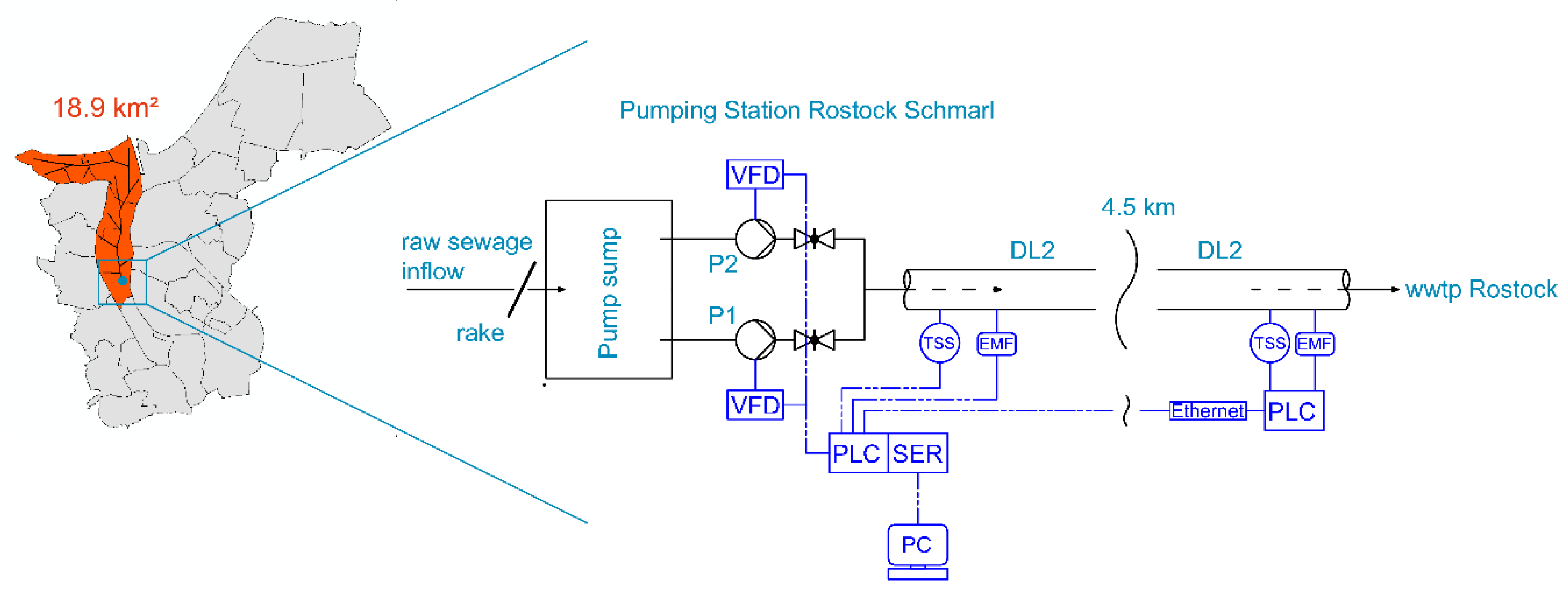
2.1. Study Side

One of the main PS in the city of Rostock (≈200000 inhabitants) is PS Rostock-Schmarl, conveying raw sewage from approx. 40000 inhabitants. A special technical feature of the upstream, usually separating sewer system is the connection to main roads storm water runoff. The storm water system itself collects runoff from roof discharge and secondary roads. Whatever the inflow condition to PS Rostock-Schmarl is, the incoming sewage is filtered at first by a rake with a wide space bar opening (20 mm) before it is transported directly to the central wastewater treatment plant (wwtp) by four pumps (each of 55 kW) in two cast iron pipelines (diameter = 600 mm), each over 4500 m length. A schematic view of the catchment area and the PS in Figure 1 illustrates the study setup.

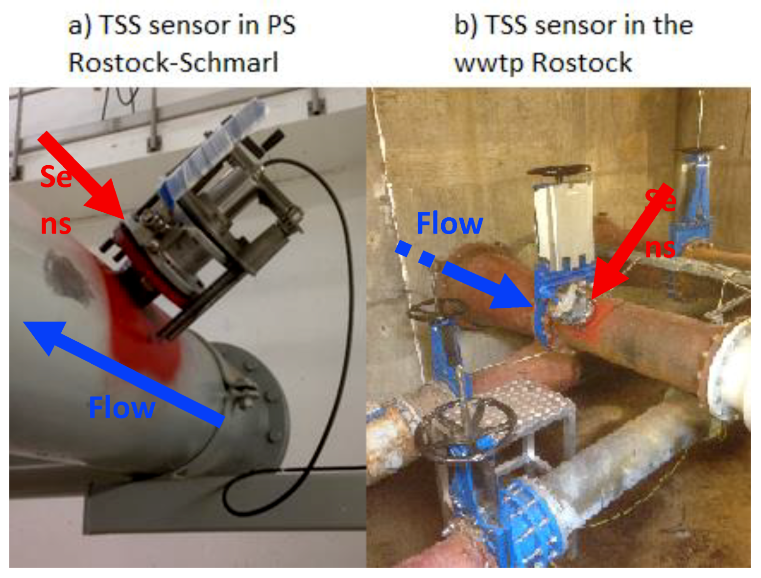
2.2. In-Situ TSS Monitoring

For a studied period of one year, pumps P1 and P2 were controlled by a PC to perform a rule based, energy saving control strategy [1,2,17]. The sediment flux was monitored by online TSS measurements at the in- and outflow side of pressure pipe DL2.

Table 1. Technical data of TSS sensors

Sensor	Controller	Parameter	Measuring Range	Installed and Measured Duration	Interval	Service	Num. of Calibration Processes	Wiper Self-Cleaning Interval
Hach Lange Solitax inline Sc	Hach Sc 200 & Sc 1000	Turbidity, TSS	0.001–4000 FNU, 0.00–150.000 mg/L	343 days installed; 292 days measured	5 s	1 per month	5 processes with 73 samples	15 min

shows the TSS sensors technical data. The sensors itself are shown in Figure 2.

Furthermore, the following parameters were monitored every 5 s over 1 year: pump sump level (m), inflow to the PS (L/s), pumps power input (kW), frequency of the VFD (F) (Hz), engine speed (min⁻¹), pressure in DL2 directly after the pump (bar), flow in DL2 (Q_pipe) (L/s).

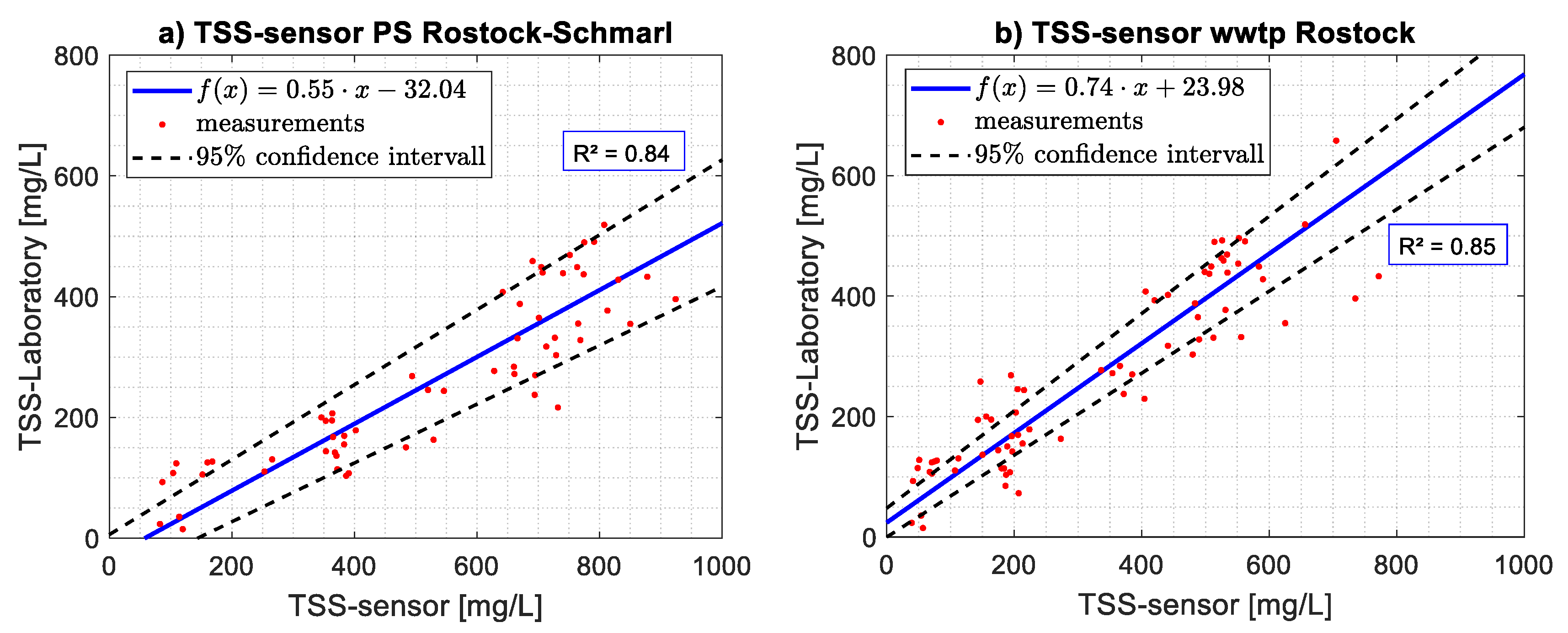
2.3. Sample-Specific Sensor Calibration

The turbidity sensors measuring principle is an infrared due scattered light technique [18]. The TSS eventually calculated from the turbidity by an internal factory calibrated formula. Commonly, diatomaceous earth is used for the internal calibration process.

To adjust the TSS sensor values to the local raw sewage composition of PS Rostock-Schmarl, a sample-specific calibration based on a correlation method was repeated 5 times, with 73 separate raw sewage samples in total. The samples are collected with a ladle from the inflow channel, just before the rake. Afterwards, the samples are filtered, according to the rakes space bar opening of 20 mm, and subsequently separated into cylinders of a small volume (2.5 L). In the second step, the TSS concentration is artificially modified to obtain different cylinders with different TSS values. Therefore, the TSS concentration is decreased by mixing several dilutions using clear water, while settling increases the TSS values. This procedure provides a wide range of TSS values for calibration process. Thus, the resulting calibration function is applicable for a broad spectrum of TSS values without extrapolation. After that, a sample is filled into the calibration cylinder and continuously mixed by a magnetic stirrer. Next, the sensors are demounted from the pressure pipe and placed into the calibration cylinder. Subsequently, three sensor TSS values are noted from the controller board. Finally, each sample is analyzed for TSS by three-fold determination in the laboratory (analysis according to [19] by filtration and weight loss).

2.4. Fit Calibration Function and Analysis of Sensor Data

Sensor data must be validated before further processing into erosion and sedimentation behavior. Various literature deals with error assessment and validation of sensor data to find a correlation function and at least a true area of measured values with respect to uncertainties (i.e., [12] or [15]). According to these publications, the determination of uncertainties was processed after the commonly used “Guide to the Expression of Uncertainty in Measurement” (GUM) [20]. Therefore, the following data analysis scheme was applied:

• Fit calibration function (TSS to TSS) with errors in y and x direction using the total least-squares regression;
• Calculate function parameters uncertainties by Monte-Carlo simulation for 95% confidence level;
• Transform original sensor data TSS_sens by the calibration function into calibrated sensor data TSS_cal;
• Remove TSS_cal values > 1.000 mg/L, based on local operators’ expertise;
• Further error assessment by Walsh’s outlier test.

First, the calibration function is performed by the total least-squares regression. By this, errors in both directions, resulting from the TSS determination inside the laboratory (y) and the TSS measurement by the sensor (x), were accounted for the optimization problem. The resulting regression function is a first order polynomial function with the slope b (-) and intercept a (mg/L). The function calculates the calibrated TSS values TSS_cal (mg/L) from the original sensor data TSS_sens (mg/L), see Equation (1).

$$f\left(TS{S}_{sens}\right)=b·TS{S}_{sens}+a$$

(1)

Second, the function parameters uncertainties are calculated for 95% confidence level by Monte-Carlo simulation in MATLAB (see also [12]). The calculation of a combined uncertainty resulting from the sensor measurement itself and the field influences (i.e., installation site) has been omitted. It is assumed, that field influences are already included in the sensor output. It is furthermore assumed that the field influence occurring during the in-pipe measurement is equal to the field influence occurring during the calibration process outside the pressure pipe.

Third, the original sensor output TSS_sens is transformed into calibrated sensor data TSS_cal to obtain the estimated TSS values by Equation (1). Furthermore, the 95% confidence interval is calculated based on the function parameters uncertainties.

Fourth, all TSS values > 1.000 mg/L are removed from the calibrated data set. The criterion based on the local operator’s expertise.

Fifth, measurement errors are cleaned by the Walsh outlier test. The test requires no specific distribution, can easily be coded, enables fast computing, and detects outliers greater and less than the remaining values.

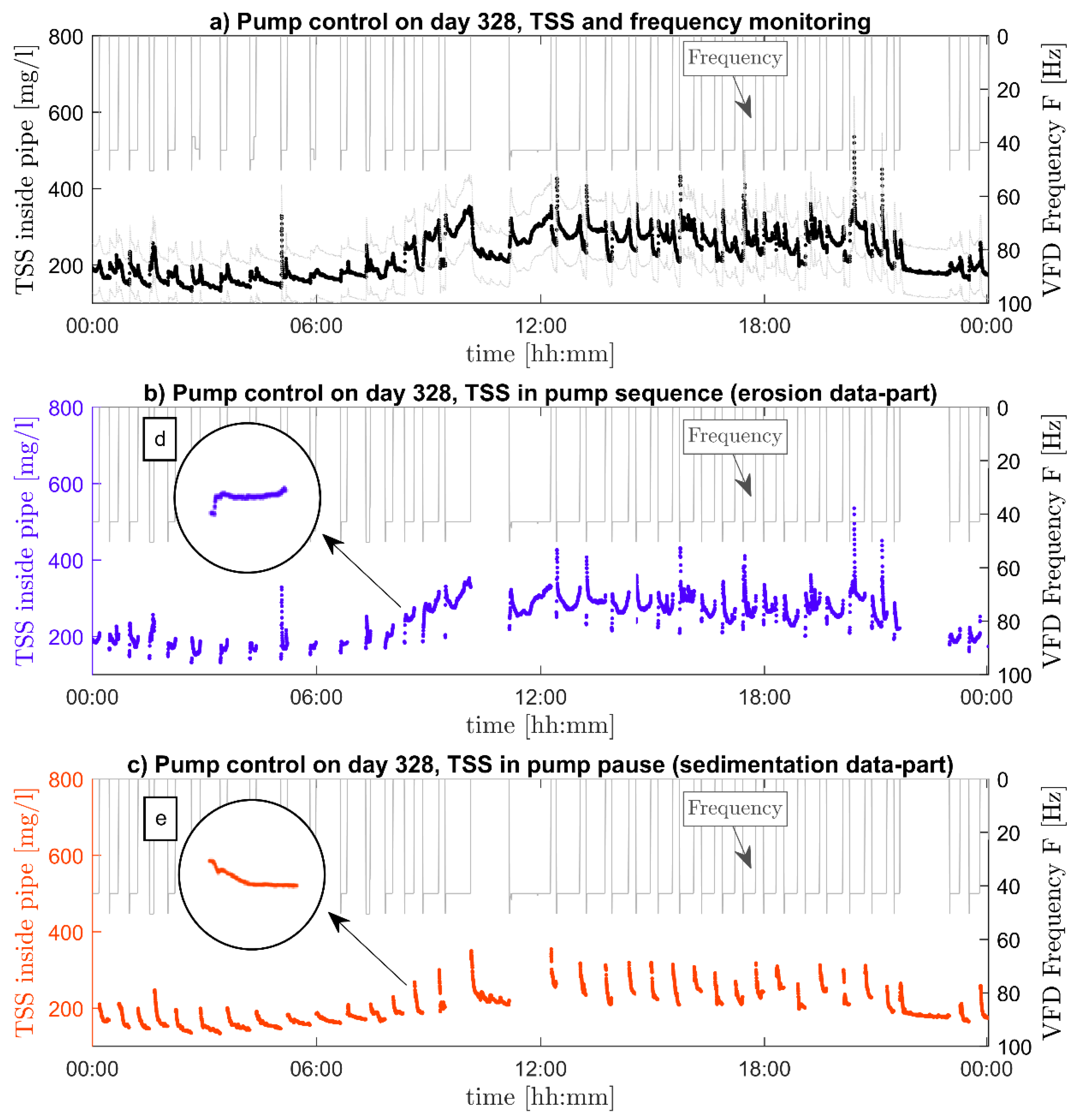
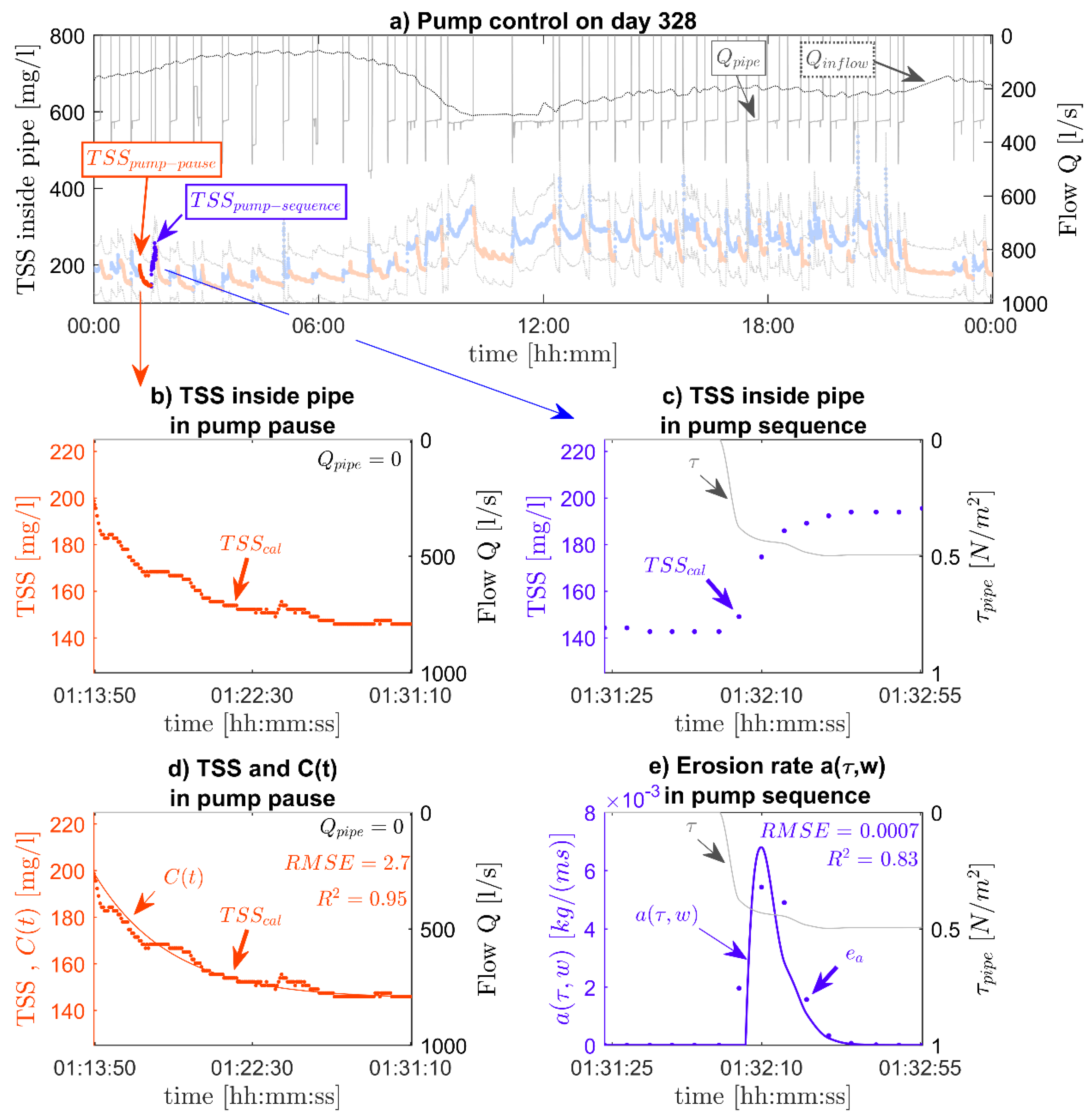
2.5. Determination of Settling- and Erosion Data

After calibration and error assessment, the final data processing followed, before determination of settling and erosion data is conducted. The transport characteristics are analyzed based on TSS sensor values in PS Rostock-Schmarl. The TSS sensor values from the central wwtp are used in Part II as reference for the sediment transport model.

The data processing scheme is visualized in Figure 3 and is described below. To maintain the data for determination, the complete data set (Figure 3a) must be split up in two parts: (i) the erosion data-part (Figure 3b), containing data while one of the two pumps is working; (ii) the sedimentation data-part (Figure 3c), containing data logged while pumps are shut off. Each data-part (erosion-part and sedimentation-part) is further split up into separate erosion (Figure 3d) and sedimentation events (Figure 3e). This is necessary, because the characterization is at least a mathematical approximation of a single erosion and sedimentation event. These single events are now the basis the mathematical description.

The sedimentation of solid fractions inside a fluid can be described by a settling velocity distribution (e.g., see [1] or [4]). However, since the turbidity sensors are not able to detect single particle fractions, the following approximation is applied. The settling events are described as a decay process, modeled by a differential Equation (2).

$$\frac{dC}{dt}=-\mathsf{\alpha }·C$$

(2)

Its solution is an exponential decay, called settling rate C(t) (mg/L), see Equation (3). With t (s), the settling duration in each pump pause, C₀ (mg/L), a fixed value relating to the first TSS concentration in each single sedimentation event, C_rest (mg/L), the final solids concentration at the end of each single setting event and the exponential decay rate α (1/s), which is the key parameter to describe the settling behavior.

$$C\left(t\right)={\mathrm{C}}_0·e^{-\alpha ·t}+C_{rest}$$

(3)

Within each time step t, a proportion of the initial TSS concentration C₀ settles to pipes invert, according to the decay rate α, which is received by solving the optimization problem in Equation (4). With n, the number of values in each settling sequence and TSS_cal (mg/L), the measured and calibrated TSS concentration inside the pressure pipe.

$$\underset{\alpha }{\min }{\displaystyle \sum }_{i=1}^n{\left(TS{S}_{cal,i}-C_i\right)}^2$$

(4)

The erosion events are described according to [1]. The measured erosion rate e_a (kg/(m s)) inside the pipe is calculated from the TSS concentration after pumps start (shown in Figure 3d), by Equation (5). With TSS_cal,i − TSS_cal,i−1 (mg/L), the TSS difference between measurements, Δt (s), the time difference between measurements and A_s (m²), the surface area of erosion (set to 1 m² for better comparability).

$$e_a=\frac{TS{S}_{cal,i}-TS{S}_{cal,i-1}}{\Delta t}·A_s$$

(5)

The measured erosion rate e_a can be described as a function of the current bed shear stress, called erosion rate a (activation of sediments) (kg/(m s)), see Equation (6). With τ_pipe (N/m²), the current bed shear stress, τ_crit (N/m²), the critical bed shear stress where erosion starts and d (s), the erosion parameter, which describes the strength of the erosion (equal to slope of the first order polynomic function).

$$a\left({\tau }_{pipe}\right)=\max \left(0,d·\left({\tau }_{pipe}-{\tau }_{crit}\right)\right)$$

(6)

τ_pipe is calculated by Equation (7), based on the fluid density ρ = 1000 (kg/m³), the flow velocity v (m/s), and the friction factor λ (calculated after the Colebrook–White equation).

$${\tau }_{pipe}=\rho ·\frac{v^2}{2}·\frac{\lambda }{4}$$

(7)

The height of τ_crit depends on several parameters, as the formerly settling duration (higher τ_crit values for longer settling duration) and the composition of the sewage (organic components raises τ_crit due to biogenic changes). For a detailed description of τ_crit see [1]. The erosion rate a is adjusted to the measured erosion rate e_a by solving the optimization problem in Equation (8).

$$\underset{d,{\tau }_{crit}}{\min }{\displaystyle \sum }_{i=1}^n{\left(e_{a,i}-a_i·w_i\right)}^2$$

(8)

To consider real life conditions inside the pressure pipe, w (kg), the current particle mass on pipe bottom is multiplied with the erosion rate a. If the sediment bed is empty (w = 0), the erosion rate a becomes zero. By solving Equation (8), the function parameter d and additionally the critical bed shear stress τ_crit is received.

3. Results and Discussion

3.1. Sensor Calibration Results

The result of the calibration processes is shown in Figure 4. The laboratory TSS correlates to each sensor TSS by a first order polynomic function.

With the resulting calibration function, the sensor values are converted into the laboratory values, before further processing. The calibration functions are fitted with a R² value of 0.84 for TSS sensor PS Rostock-Schmarl and with a R² value of 0.85 for TSS sensor at the central wwtp Rostock. As found in literature, usual calibration functions used same functions with R² values between 0.83 and 0.92 [8] (calibration to turbidity) or, as already summarized in [15], between 0.80 and 0.95 [15] (calibration to turbidity). Reference [9] obtained a calibration function, for the same sensor used in this study, with a R² value of 0.94.

As one can see in the functions slope b, the measured values of both sensors are too high. Furthermore, we obtained two different calibration functions, although both sensors are identically and the same TSS samples used for calibration. A reason might be found in the differences to the internal calibration process. The used material for internal calibration differs from the raw sewage, as well as the calibration cylinder geometry. Another reason might be in the different controller devices used for the sensors. Differences in the internal signal processing may cause different values.

3.2. Evaluation of the Erosion and Settling Approximation

The evaluation of the raw sewage erosion and settling characteristics is based on an enormous amount of data. In sum, the TSS sensor in PS Rostock-Schmarl recorded 4238121 values (5 s interval over 1 year). 2203618 values of them account for erosion sequences and 2034503 values for settling sequences. The total number of single erosion sequences amount to 6653, while 6733 single settling events are recorded. This leads on average to ≈24 erosion and ≈24 settling events per day. Hence, the pumps are working every half hour for 30 min.

For each single erosion and settling event, a mathematical function is adjusted to the measured TSS values, automatically by a MATLAB code. This enables a fast, uncomplicated, and reproducible processing. The function itself is given by the settling rate C(t), Equation (3), and by the erosion rate, written as a(τ,w) (following Equation (8)).

First, we will evaluate the approximations of the erosion and settling processes. Figure 5 evaluates the fit results graphically. In Figure 5a, all measured erosion rates e_a are plotted versus all fitted erosion rates a(τ,w). A perfect fit is given by f(x) = x or a(τ,w) = e_a. For the majority of erosion values, a(τ,w) follows the perfect fit course with deviations above and below. The fitting results are moderate. R² value of >=0.9 having 7.3% of the total approximations (n = 481 single events), 33.5% (n = 2100) were fitted with R² values of >=0.75, while R² values of >=0.5 having 54% (n = 3603). So the mathematical approximation by the erosion rate a(τ,w) is suitable to describe the real process of erosion. Because of the similar up- and downward deviation, a balance is assumed.

Figure 5b shows all measured TSS values in the pump pauses versus all approximations by C(t). Here, the majority of the values are located just below the perfect fit line. Accordingly, the settling process is slightly overestimated. In contrast to erosion, a better fit is achieved for settling. R² values of >=0.9 having 31% of the total approximations (n = 2084 single events), 58.4% (n = 3934) were fitted with R² values of >=0.75 and R² values of >=0.5 having 76% (n = 5161).

Both models are able to describe real world conditions appropriately. The deficits in the erosion approximation may result from its dynamic process. If the TSS sensor measures a value immediately when the pump starts, it takes 5 s of pumping until the next value is recorded. Within these 5 s, some sediments are already eroded. This means that a shorter measuring interval is recommended for the erosion process in later studies. Furthermore, the limited flexibility of the erosion rate a(τ,w) itself, as it is based on a first order polynomic function (see Equation (6)), contributes to its moderate results. A transformation into a power function (e.g., $a\left({\tau }_{pipe}\right)=d·{\left({\tau }_{pipe}-{\tau }_{crit}\right)}^p$) leads to slightly better results but with larger computation effort, e.g., for a sediment transport simulation.

3.3. Settling and Erosion Characteristics Inside the Pressure Pipe Under Dry Weather Inflow

Transport characteristics are essentially dealing with numerical simulation of sediment transport in open channel flow or dimensioning of facilities and treatment plants or solids transport inside pressure pipes. Hence, the in-pipe measurement helps to improve accuracy of the transport characterization and widen the spectrum of results substantially. Furthermore, it serves as a comparison to laboratory (ex-situ) results, obtained in [1,2].

The example in Figure 6a shows a typical situation in PS Rostock-Schmarl, comparable to usual urban drainage pumping stations. The diurnal course of TSS is separated, according to Figure 3, into erosion events (blue) and settling events (red). The diurnal course of the raw sewage inflow is presented by Q_inflow and the resulting pump flow by Q_pipe (right axes).

The TSS values during the night are relatively low. They reach a minimum of ≈200 mg/L at about 03:30 a.m. (in pump sequence) before starting to increase from 06:00 a.m. to 12:00 a.m. up to 400 mg/L. Peaks up to 600 mg/L may be the result of the sensor wiper, cleaning the sensor from heavy dirt (e.g., paper shreds). The TSS course follows the inflow course of Q_inflow. Hence, there is a relationship between TSS and Q_inflow. Low inflow results in low TSS values and vice versa. It results from the water usage and the hydraulic conditions in the upstream sewers. An increased solids amount reaching the PS by increased water consumption (stool, cooking, etc.). Furthermore, high water consumption raises the hydraulic performance in the upstream sewers and erodes deposits.

The TSS course is characterized by two long settling periods. A specific settling characteristic becomes clear within these two periods. The TSS first decreases rapidly but then slows down. This is also addressed in [2], where the same characteristic was found. Accordingly, an exponential function (see Equation (3)) describes this process most appropriate. Consequently, the TSS never decreases to full extend in pump pauses.

Figure 6b shows an exemplary settling course in detail, while Figure 6d shows the resulting settling rate. Although the pump pause only takes ≈17 min, the TSS inside the fluid reduces from ≈200 mg/L at about 27.5% to ≈145 mg/L. The effect of the exponential decrease shows the risk of forming a consolidated sediment layer inside the pressure pipe, even in short pump pauses. If sediments erode incompletely within the subsequent pump sequences, permanent deposits are likely to develop.

Figure 6c,e shows the subsequent erosion sequence and the determination of the erosion rate. The erosion process always forms an s-shaped curve (Figure 6c). This shape is characterized by a restrained start and is followed by an increased erosion. The inflection point of the s-curve marks the beginning of the decrease phase with a weakening erosion. The formerly settled solids are completely eroded from ≈145 mg/L up to ≈200 mg/L within 30 s. The resulting erosion rate (Figure 6e) shows an abrupt increase at the beginning, which is due to its moderate fitting results (R² = 0.83). Similar to the smoother decline at the end of the erosion event, a more gradual increase is assumed for the beginning. The maximum erosion appears at ≈0.43 N/m² and so, before the maximum shear stress level of ≈0.5 N/m² is reached. A further increase of shear stress (feasible by parallel pumping of P1 and P2) would not result in further solids erosion, as the maximum erosion level is already reached and the decline remarks the emptying of the sediment layer.

3.4. Comparison to Laboratory (Ex-Situ) Results

The results of the ex-situ laboratory experiments in [1] are similar to the in-situ measured erosion processes in this study. Both methods show the typical s-curve while eroding solids. Hence, the resulting erosion rates are quite similar. Especially the calculated duration for a complete resuspension in [1], with regard to similar hydraulic conditions (≈ 0.5 N/m² bed shear stress), is nearly equal to real world processes (duration ≈ 30 s). Thus, both methods (in-situ and ex-situ) are applicable to determine the erosion characteristics of raw sewage.

However, the in-situ characterization of the erosion events is much harder compared to the ex-situ method in [1], as the solids inside the pipe are moving in two main directions (upward and forward, micro-effects ignored). Therefore, next to the formerly settled solids directly under the TSS sensor, particles settled at the upstream section of the pressure pipe affecting the measurement. A closed reaction chamber, within the ex-situ experiments in [1], simplifies the measurement extremely, as the erosion process of a controlled suspension is detected. This may be another reason for the moderate fitting results (see previous chapter).

A direct comparison to the ex-situ settling experiments in [2] is not possible. The in-situ method measures the TSS reduction in the fluid phase (by a calibrated turbidity sensor) and the ex-situ method measures the total mass increase at the bottom of a cylinder (by weight loss). Furthermore, the mathematical description differs from [2]. However, by converting the cumulative growth from [2] into the fluids particle loss, an equal course to the settling rate is found (exponential shape). Furthermore, both methods counted approximately the same solids amount after similar settling durations. 25.4% of solids mass settle in a laboratory test within 17 min while approximately 27.5% of the solids settle within the same duration inside the pressure pipe.

A continuous measurement of solids decrease inside a fluid phase by a sensor is by far much easier and more worthwhile, than a manually ex-situ determination of solids mass growth. The laboratory experiment lags behind the sensor determination, because of the high effort in designing and construction, sampling, the experimental conduction and mass detection. The continuous and automated in-situ measurement scores by a unique installation, simple maintenance, and calibration, high-resolution measurement (5 s interval) and automated data processing.

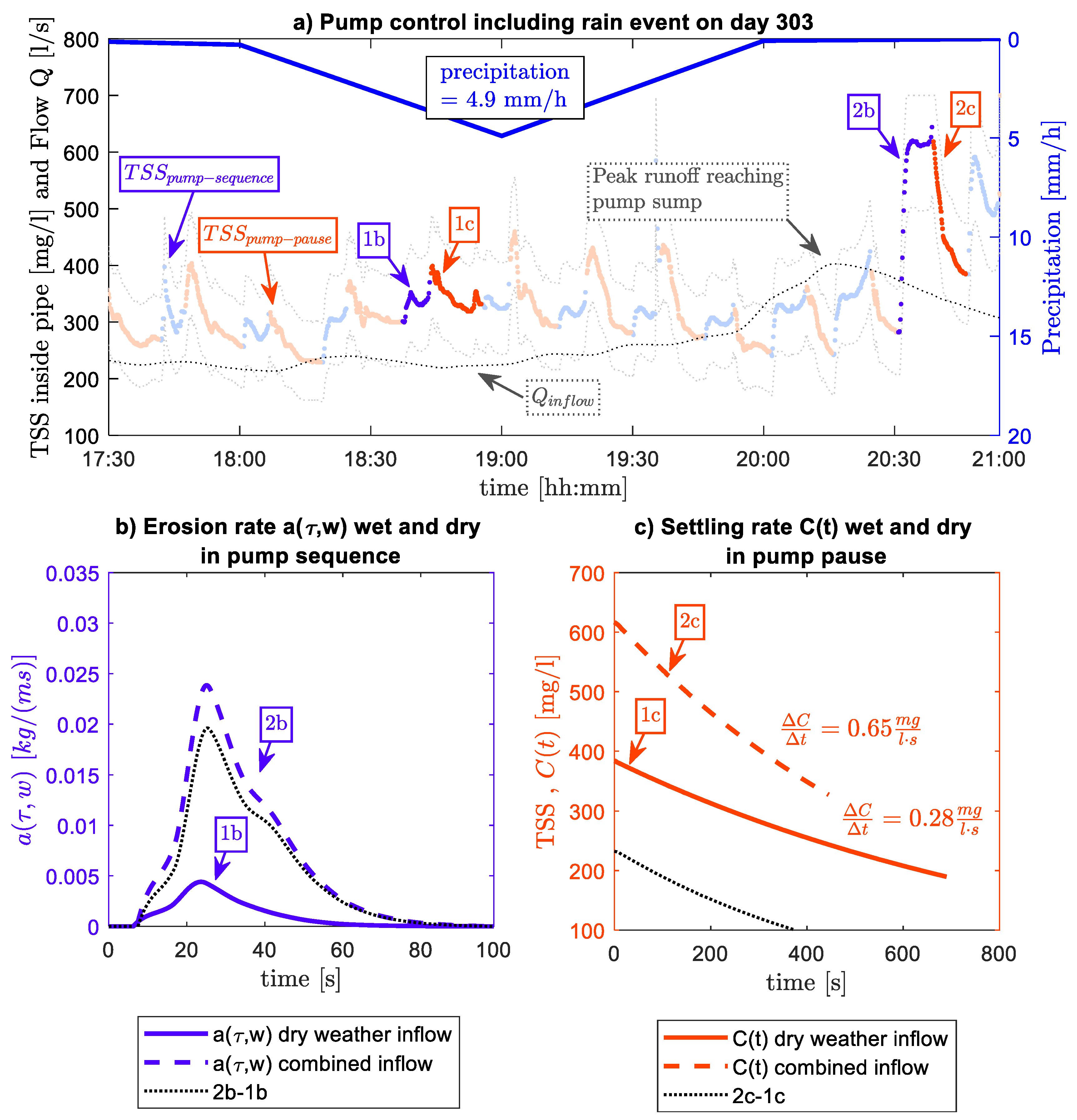
3.5. Effect of Storm Water Inflow to Settling and Erosion Characteristics

Due to the connected road runoff, a changed erosion and sedimentation behavior is assumed by storm water inflow. Several storm events were measured during the study period. One example is shown in Figure 7. Figure 7a shows a rain event at 07:00 p.m. with 4.9 mm/h precipitation (right axis). The inflow curve shows the storm runoff slowly reaching the pump sump (see Q_inflow, left axis). The TSS course (left axis) is separated into erosion (blue) and sedimentation sequences (red). The TSS concentration increases significantly up to ≈600 mg/L after the peak runoff reaches the pump sump. Figure 7b compares a dry weather inflow erosion rate (1b) with a storm water erosion rate (2b). The maximum erosion increases with the storm inflow almost by a factor of five. One reason is the storm runoff composition. Solids (sand, tire abrasion, etc.) are washed off from roads and entering the sewer. Furthermore, the increased discharge erodes pre-settled and consolidated deposits and spills a mixture of runoff solids and sewer solids to the PS.

The following sedimentation process (2c) is significantly different compared to dry weather conditions (1c), accordingly. The increased TSS inflow raises the start value of sedimentation (C₀) from ≈400 mg/L up to >600 mg/L. A better comparison of the settling processes is provided by the mean decrease, which is defined as the difference quotient in the interval [t₁;t_end], see Equation (9).

$$\frac{\Delta C}{\Delta t}=\frac{\left|C\left(t_{end}\right)-C\left(t_1\right)\right|}{t_{end}-t_1}$$

(9)

In this example, the TSS concentration decreases under dry weather inflow (1c) with 0.28 mg/(L s), while under storm water inflow (2c) twice as fast with 0.65 mg/(L s). Hence, next to the solids concentration, the solids composition changes as well. This indicated an increased inflow of heavier particles (runoff- and sewer solids). The total mean decrease under dry weather inflow, calculated over 4520 settling events, is 0.23 mg/(L s), while under storm water inflow 0.9 mg/(L s) (calculated over 9 rain events). Therefore, a more than 3.5-times faster settling can be assumed under storm water inflow. This increases the risk of blockages significantly. The risk is highest when the solids enter the pressure pipe. The storm runoff reaches the pump sump 1 h after the rain event and enters the pressure pipe usually 1.5 h after the rain event. The accumulation of particles on roads and the deposition of solids inside the sewers increases with longer dry periods. This is due to missing wash-off and limited discharge. Hence, the risk of blockages in the pressure pipe increases for short but intensive rain events after long dry weather periods. However, this effect is not investigated within this study.

3.6. Comparison to Laboratory (Ex-Situ) Results

A changed sedimentation behavior is already recognized in [2]. Samples, collected under storm water inflow settling significantly faster. Comparable laboratory tests showing a mean decrease for storm water samples by 1.1 mg/(L s), while 0.18 mg/(L s) for dry weather samples.

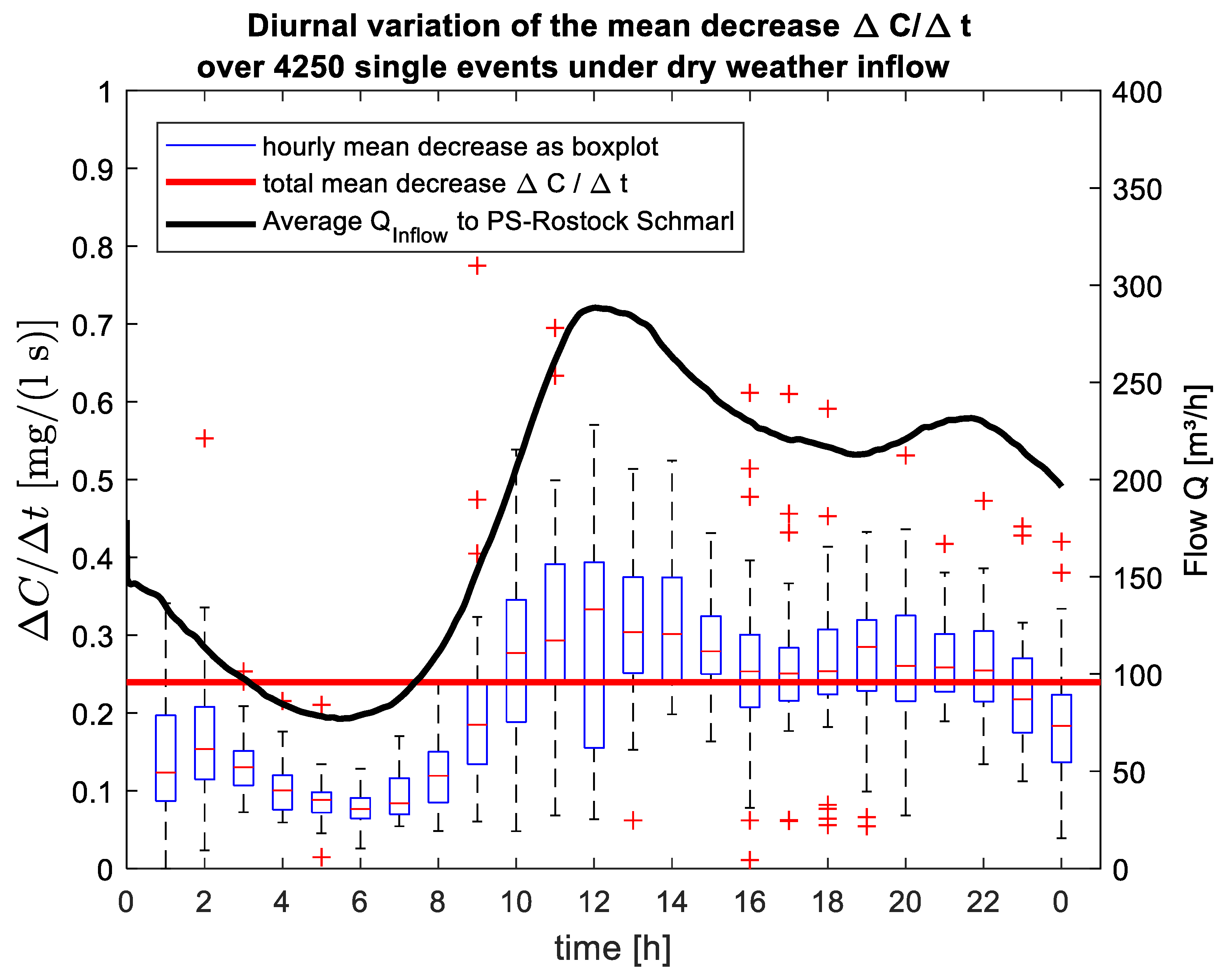
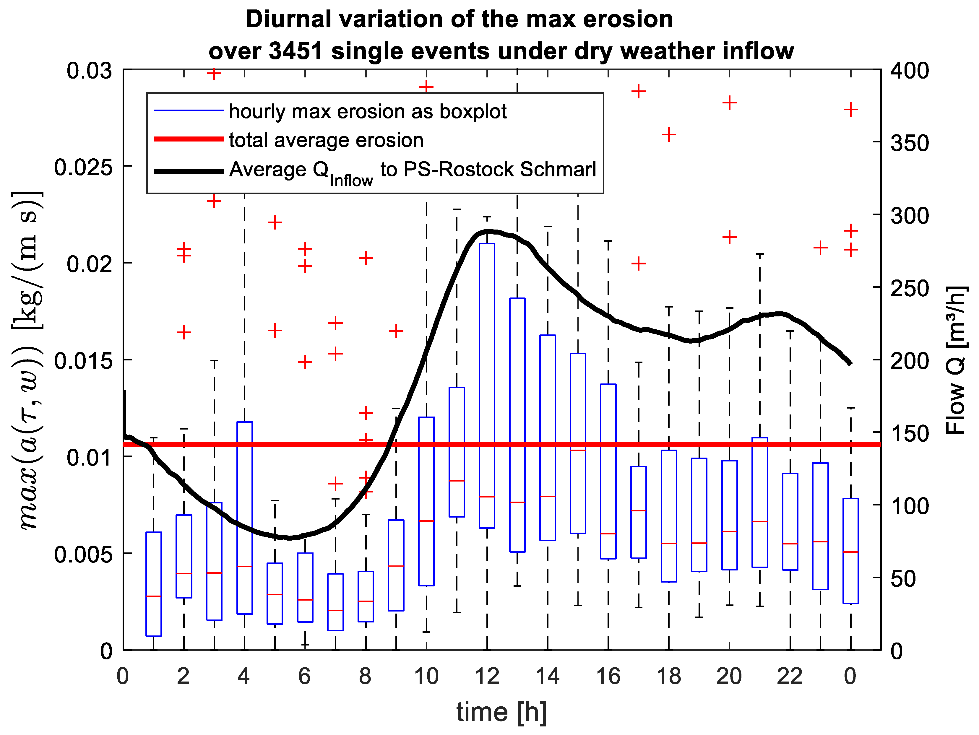
3.7. Diurnal Variation Settling and Erosion

Settling and erosion characteristics are changing not only with storm water inflow. As already mentioned previously, TSS follows the inflow course. As settling and erosion depends on TSS, their behavior follows TSS and consequently inflow. Hence, changes are also assumed due to the diurnal variation of inflow. This relation is shown in Figure 8 and Figure 9. Both showing the average diurnal variation of inflow (black line), including boxplots for hourly mean decrease (Figure 8) and hourly maximum erosion per event (Figure 9).

Both indicators (mean decrease and maximum erosion) follow the up- and downward course of inflow. Especially in the morning, the swage is characterized by slow settling processes (<0.1 mg/(L s)) and low erosion rates (<0.0025 kg/(m s)). This can be explained by the reduced water usage in the night (reduced solids input, reduced hydraulic performance in upstream sewers). Vice versa, due to a high water usage in morning hours, peak inflows reaching the PS at lunch and changing the sewage to a faster settling mixture (up to 0.5 mg/(L s)). Accordingly, the erosion rate increases up to 0.02 kg/(m s). The increased erosion rate is a result of a faster settling process. The more solids settle within the pump pauses, the more solids can be eroded in the pump phases. Hence, the erosion rate depends on the pump pause duration. Longer pump pauses generally occur in the night or in the morning with low inflow rates (see [2]). Nevertheless, due to a slow settling sewage, the erodible amount of solids is low. The erodible amount is at its peak, when the settling process is fast (usually at midday), irrespective to pump pause duration. Concluding, the sewage settling characteristics (slow or fast) determine the deposits formation more than the duration of the pump pauses.

4. Conclusions

The paper presents a continuous in-situ TSS measurement system for raw sewage inside a pressure pipe and the determination and characterization of settling and erosion behavior based on high-resolution sensor data. Ultimately, the following findings are concluded:

• The installed sensors are suitable for supervision of TSS fluxes inside sewage pressure pipes;
• Periodically calibration and maintenance of TSS sensors result in reliable data;
• TSS sensor data allow for a characterization of solids sedimentation and erosion behavior;
• Measured in-situ erosion and settling results are similar to ex-situ (laboratory) results;
• Settling accelerates with high inflow rates (storm water inflow, diurnal inflow peaks) and decelerates with low inflow (reduced TSS inflow in night phases);
• Erosion rate increases and decreases based on the available amount of solids, hence, with changing settling behavior;
• Solids are eroded before maximum shear stress level reached

Within continuous sensor measurements, a huge amount of data is generated. Especially with regard to urban water simulations, this provides the opportunity for precise calibration up to specified scenarios. Hence, changes of solids erosion and sedimentation caused by storm water inflows of various intensity or by the diurnal inflow can be dynamically implemented into hydraulic models by providing a wide spectrum of appropriate calibration parameters. The presented results are primarily used for a sediment transport simulation inside the pressure pipe of PS Rostock-Schmarl, presented in Part II of this publication: “Sediment Transport in Sewage Pressure Pipes, Part II: 1D Numerical Simulation”.

References

1. Rinas, M.; Tränckner, J.; Koegst, T. Erosion characteristics of raw sewage: Investigations for a pumping station in northern Germany under energy efficient pump control. Water Sci. Technol. 2018, 78, 1997–2007. [Google Scholar] [CrossRef] [PubMed]
2. Rinas, M.; Tränckner, J.; Koegst, T. Sedimentation of Raw Sewage: Investigations for a Pumping Station in Northern Germany under Energy-Efficient Pump Control. Water 2019, 11, 40. [Google Scholar] [CrossRef]
3. Seco, I.; Gómez Valentín, M.; Schellart, A.; Tait, S. Erosion resistance and behaviour of highly organic in-sewer sediment. Water Sci. Technol. 2014, 69, 672–679. [Google Scholar] [CrossRef] [PubMed]
4. Gromaire, M.C.; Kafi-Benyahia, M.; Gasperi, J.; Saad, M.; Moilleron, R.; Chebbo, G. Settling velocity of particulate pollutants from combined sewer wet weather discharges. Water Sci. Technol. 2008, 58, 2453–2465. [Google Scholar] [CrossRef] [PubMed]
5. Chebbo, G.; Gromaire, M.-C.; Lucas, E. Protocole VICAS: Mesure de la vitesse de chute des MES dans les effluents urbains. TSM Tech. Sci. Methodes Génie Urbain Génie Rural 2003, A98, 39–49. [Google Scholar]
6. Regueiro-Picallo, M.; Naves, J.; Anta, J.; Suárez, J.; Puertas, J. Monitoring accumulation sediment characteristics in full scale sewer physical model with urban wastewater. Water Sci. Technol. 2017, 76, 115–123. [Google Scholar] [CrossRef] [PubMed]
7. Xu, Z.; Wu, J.; Li, H.; Liu, Z.; Chen, K.; Chen, H.; Xiong, L. Different erosion characteristics of sediment deposits in combined and storm sewers. Water Sci. Technol. 2017, 75, 1922–1931. [Google Scholar] [CrossRef] [PubMed]
8. Bersinger, T.; Le Hécho, I.; Bareille, G.; Pigot, T.; Lecomte, A. Continuous Monitoring of Turbidity and Conductivity in Wastewater Networks. Rev. Des Sci. De L’eau 2015, 28, 9. [Google Scholar] [CrossRef]
9. Bersinger, T.; Le Hécho, I.; Bareille, G.; Pigot, T. Assessment of erosion and sedimentation dynamic in a combined sewer network using online turbidity monitoring. Water Sci. Technol. 2015, 72, 1375–1382. [Google Scholar] [CrossRef] [PubMed]
10. Lacour, C.; Joannis, C.; Chebbo, G. Assessment of annual pollutant loads in combined sewers from continuous turbidity measurements: Sensitivity to calibration data. Water Res. 2009, 43, 2179–2190. [Google Scholar] [CrossRef] [PubMed]
11. Métadier, M.; Bertrand-Krajewski, J.-L. From mess to mass: A methodology for calculating storm event pollutant loads with their uncertainties, from continuous raw data time series. Water Sci. Technol. 2011, 63, 369–376. [Google Scholar] [CrossRef] [PubMed]
12. Métadier, M.; Bertrand-Krajewski, J.-L. The use of long-term on-line turbidity measurements for the calculation of urban stormwater pollutant concentrations, loads, pollutographs and intra-event fluxes. Water Res. 2012, 46, 6836–6856. [Google Scholar] [CrossRef] [PubMed]
13. Lacour, C.; Joannis, C.; Gromaire, M.-C.; Chebbo, G. Potential of turbidity monitoring for real time control of pollutant discharge in sewers during rainfall events. Water Sci. Technol. 2009, 59, 1471–1478. [Google Scholar] [CrossRef] [PubMed]
14. Sun, S.; Barraud, S.; Castebrunet, H.; Aubin, J.-B.; Marmonier, P. Long-term stormwater quantity and quality analysis using continuous measurements in a French urban catchment. Water Res. 2015, 85, 432–442. [Google Scholar] [CrossRef] [PubMed]
15. Bertrand-Krajewski, J.-L. TSS concentration in sewers estimated from turbidity measurements by means of linear regression accounting for uncertainties in both variables. Water Sci. Technol. 2004, 50, 81–88. [Google Scholar] [CrossRef] [PubMed] [Green Version]
16. Bertrand-Krajewski, J.-L.; Bardin, J.-P. Evaluation of uncertainties in urban hydrology: Application to volumes and pollutant loads in a storage and settling tank. Water Sci. Technol. 2002, 45, 437–444. [Google Scholar] [CrossRef] [PubMed]
17. Knubbe, A.; Fricke, A.; Ecktädt, H.; Neymeyr, K.; Schwarz, M.; Tränckner, J. Energieeffizienter Betrieb von Abwasserfördersystemen Energy efficient strategies for wastewater pumping systems. Gwf. Wasser|Abwasser 2014, 155, 640–646. [Google Scholar]
18. HACH-LANGE GmbH. SOLITAX sc User Manual: Edition 4A; HACH LANGE GmbH: Düsseldorf, Germany, 2009; Available online: https://de.hach.com/asset-get.download.jsa?id=25593604876 (accessed on 12 October 2019).
19. Deutsches Institut für Normung e.V. (DIN). Deutsche Einheitsverfahren zur Wasser-, Abwasser- und Schlammuntersuchung; Summarische Wirkungs- und Stoffkenngrößen (Gruppe H); Bestimmung des Gesamttrockenrückstandes, des Filtrattrockenrückstandes und des Glührückstandes (H 1) (German Standard Methods for the Examination of Water, Waste Water and Sludge; General Measures of Effects and Substances (Group H); Determination of the Total Solids Residue, the Filtrate Solids Residue and the Residue on Ignition (H 1)); DIN ISO 38414-S; Beuth Verlag GmbH: Berlin, Germany, 1987. [Google Scholar]
20. International Organization for Standardization (ISO). Uncertainty of Measurement—Part 3: Guide to the Expression of Uncertainty in Measurement (GUM:1995); ISO/IEC Guide 98-3:2008(E); ISO: Geneva, Switzerland, 2008. [Google Scholar]
Figure 1. Visualization of the catchment area (18.9 km2) in Rostock (Germany) including a schematic view of the control and monitoring system during the study. The raw sewage inflow passes the rake and is collected inside the pump sump. Pumps P1 and P2 then conveying the raw sewage directly to the central wwtp in pressure pipe 2 (DL2). P1 and P2 are controlled over a variable-frequency drive (VFD) from a PC (connected over a serial port (SER) to the programmable logic controller (PLC)). The VFD adjusts pumps motor speed according to the control strategy [1,2,17]. All values from TSS sensors (TSS) and electromagnetic flowmeters (EMF) are stored in the PC.
Water 11 02125 g001
Figure 2. TSS sensors for monitoring sediment flux in pressure pipes. (a) TSS sensor in PS Rostock-Schmarl at the pressure side of the pump. (b) TSS sensor in the central wwtp Rostock at the outflow side of the pressure pipe.
Water 11 02125 g002
Figure 3. Data separation scheme: monitored TSS data (a) is split into an erosion- (b) and a sedimentation part (c). Frequency data from both VFD (for P1 and P2) is used as decision criterion for data separation (if VFD1 and VFD2 = 0, then settling sequence, else erosion sequence). The separation into single erosion (d) and sedimentation events (e) is based on a time difference between each value. If the time difference is larger the logging interval of 5 s (see Table 1), a single event is detected and separated.
Water 11 02125 g003
Figure 4. Calibration functions for calculating laboratory TSS values from in-situ measured sensor TSS values, including goodness of fit (R2) and 95% confidence interval. (a) For TSS sensor in PS Rostock-Schmarl. (b) For TSS sensor at the central wwtp Rostock.
Water 11 02125 g004
Figure 5. Evaluation of the erosion and settling approximation. (a) All measured erosion rates ea vs. all mathematical approximations by a(τ,w). (b) All measured settling events inside the pipe vs. all mathematical approximations by C(t).
Water 11 02125 g005
Figure 6. Monitored data in PS Rostock-Schmarl for day 328 (a) including exemplary erosion and settling determination scheme (be). (a) Qinflow and Qpipe (right axis) and TSS sensor data including 95% confidence levels (left axis). (b) Settling event: TSS values (TSScal) after pumps stop in the night. (c) Erosion event: TSS values (TSScal) after pumps start at night. (d) Settling event determination: TSS values (TSScal) and approximated settling rate C(t) including fit results. (e) Erosion event determination: erosion rate ea and approximated erosion rate a(τ,w) including fit results.
Water 11 02125 g006
Figure 7. Effect of storm water inflow to erosion and sedimentation. (a) Qinflow and TSS data (both on left axis) during rainfall event from 06:00 p.m. to 08:00 p.m. with a peak of 4.9 mm/h (right axis). (b) Erosion rate a(τ,w) during storm water inflow (2b) compared to dry weather inflow (1b). (c) Settling rate C(t) during storm water inflow (2c) compared to dry weather inflow (1c) including mean decrease ∆C/∆t. The German Weather Service (DWD) provides the precipitation data.
Water 11 02125 g007
Figure 8. Diurnal variation of the mean decrease ∆C/∆t (boxplots) including total mean decrease over 4250 single settling events (red line) and the average Qinflow for dry weather conditions (black line).
Water 11 02125 g008
Figure 9. Diurnal variation of the max erosion (boxplots) including total average erosion over 3451 single erosion events (red line) and the average Qinflow for dry weather conditions (black line).
Water 11 02125 g009