A Depression-Based Index to Represent Topographic Control in Urban Pluvial Flooding


1
School of Geography and Planning, Sun Yat-sen University, Guangzhou 510275, China
2
Guangdong Provincial Engineering Research Center for Public Security and Disaster, Guangzhou 510275, China
3
Department of Geography and Geographic Information Science, University of Cincinnati, Cincinnati, OH 45221, USA
4
Department of Ecological Engineering, Guangdong Eco-Engineering Polytechnic, Guangzhou 510520, China
5
School of Geographic Sciences, Guangzhou University, Guangzhou 510006, China
*
Authors to whom correspondence should be addressed.
Water 2019, 11(10), 2115; https://doi.org/10.3390/w11102115
Submission received: 30 August 2019
/
Revised: 1 October 2019
/
Accepted: 9 October 2019
/
Published: 12 October 2019
(This article belongs to the Section Urban Water Management)
Abstract
:Extensive studies have highlighted the roles of rainfall, impervious surfaces, and drainage systems in urban pluvial flooding, whereas topographic control has received limited attention. This study proposes a depression-based index, the Topographic Control Index (TCI), to quantify the function of topography in urban pluvial flooding. The TCI of a depression is derived within its catchment, multiplying the catchment area with the slope, then dividing by the ponding volume of the depression. A case study is demonstrated in Guangzhou, China, using a 0.5 m-resolution Digital Elevation Model (DEM) acquired using Light Detection and Ranging (LiDAR) technology. The results show that the TCI map matches well with flooding records, while the Topographic Wetness Index (TWI) cannot map the frequently flooded areas. The impact of DEM resolution on topographic representation and the stability of TCI values are further investigated. The original 0.5 m-resolution DEM is set as a baseline, and is resampled at resolutions 1, 2, 5, and 10 m. A 1 m resolution has the smallest TCI deviation from those of 0.5 m resolution, and gives the optimal results in terms of striking a balance between computational efficiency and precision of representation. Moreover, the uncertainty in TCI values is likely to increase for small depressions.
1. Introduction
Urban pluvial flooding is defined by the Federal Emergency Management Agency (FEMA) of the United Sates as “the inundation of property in a built environment, particularly in more densely populated areas, caused by rain falling on increased amounts of impervious surfaces and overwhelming the capacity of drainage systems.” [1] Increases in both the frequency of extreme rainfalls and impervious surfaces in urban built environments have aggravated the situation of urban pluvial flooding. The roles of rainfall, impervious surfaces, and drainage systems in urban pluvial flooding are highlighted in this definition, and have also been confirmed by extensive studies [2,3,4,5,6]. Nevertheless, topography should also be underlined because of its significant effect on the direction and velocity of surface runoff. Topographic control is boosted under extreme rainfall, because permeable surfaces become saturated with water quickly, and runoff is generated at virtually the same rate as that on the impervious surfaces [7].
Topographic control in fluvial flooding has been represented by topographic indicators, such as Topographic Wetness Index (TWI) in the original form [8,9,10] and the modified form [11,12], downslope index [13], Height Above Nearest Drainage (HAND) [14], and Geomorphic Flood Index (GFI) [15]. In terms of the roles of topographic indicators and hydraulic models in flood susceptibility analyses, hydraulic models such as HEC-RAS [16], LISFLOOD-FP [17], FloodMap [18,19], Cellular Automata [20], and WOLF 2D [21,22] give more information about the dynamic process of flooding, at the cost of detailed data for model calibration and validation, and intensive computation, which makes it challenging for assessments over large areas [23,24]. Although topographic indicators cannot describe the flooding process, their capabilities have been shown to be acceptable in delineating flood-prone areas [23,24,25,26,27]. Applying topographic indicators relies on the determination of their thresholds, which can be trained to achieve the best fitting to flooding records using machine learning methods, like Logistic Regression, Support Vector Machine, Random Forest, and naive Bayes estimation [28,29,30,31,32,33,34,35]. Moreover, using topographic indicators is more feasible due to their relatively low computational cost compared to hydraulic models, and the increasing availability of high-resolution Digital Elevation Models (DEMs) [36,37,38].
However, these topographic indicators cannot be directly applied to the analysis of urban pluvial flooding, which has a driving mechanism which is distinct from fluvial flooding. The hazard source of fluvial flooding is river networks; as a consequence, flood-prone areas are spatially connected to rivers. This rule can be applied to decide whether the spatial pattern of floods is reasonable. Unfortunately, the rule doesn’t work for urban pluvial flooding, because this kind of flooding can occur in any low-lying place. A study conducted in Illinois, U.S., reported that over 90% of pluvial flooding damage claims from 2007 to 2014 had been from beyond the mapped floodplain [39]. Similar results were reported by another study in Guangzhou, China, based on historical records from 2009 to 2015 [40]. As a result, an alternative topographic index is required for the analysis of urban pluvial flooding.
Urban pluvial flooding only occurs in depressions, which hold storm water that exceeds the capacity of urban drainage systems [41,42,43]. Depressions are low-lying areas surrounded by higher places, and can be identified using Geographic Information Science (GIS) analysis and a high-resolution DEM. Surface runoff driven by gravity flows towards and accumulates in depressions, and spills downstream once the depressions are completely filled. Therefore, it’s better to take depressions as the units of analysis, rather than a single raster cell. As illustrated by an example of cell-based TWI in the Section 3, there is no spatially-explicit pattern for the distribution of TWI values with regard to the locations of historic flooded areas. In order to avoid this problem, this study proposes a depression-based index, the Topographic Control Index (TCI), to describe topographic control on urban pluvial flooding. The resulting flood susceptibility map excludes non-depression area and highlights the depressions.
In Section 2, the conceptual framework and workflow of the new index, the TCI, are illustrated. A results analysis is described in the Section 3, which includes TCI mapping and validation, a performance comparison with cell-based TWI, and a discussion of the impact of DEM resolution. The applicability and shortcomings of the new index are discussed in Section 4, and conclusions are summarized in Section 5.
2. Materials and Methods
2.1. Conceptual Framework of Topographic Control Index (TCI)
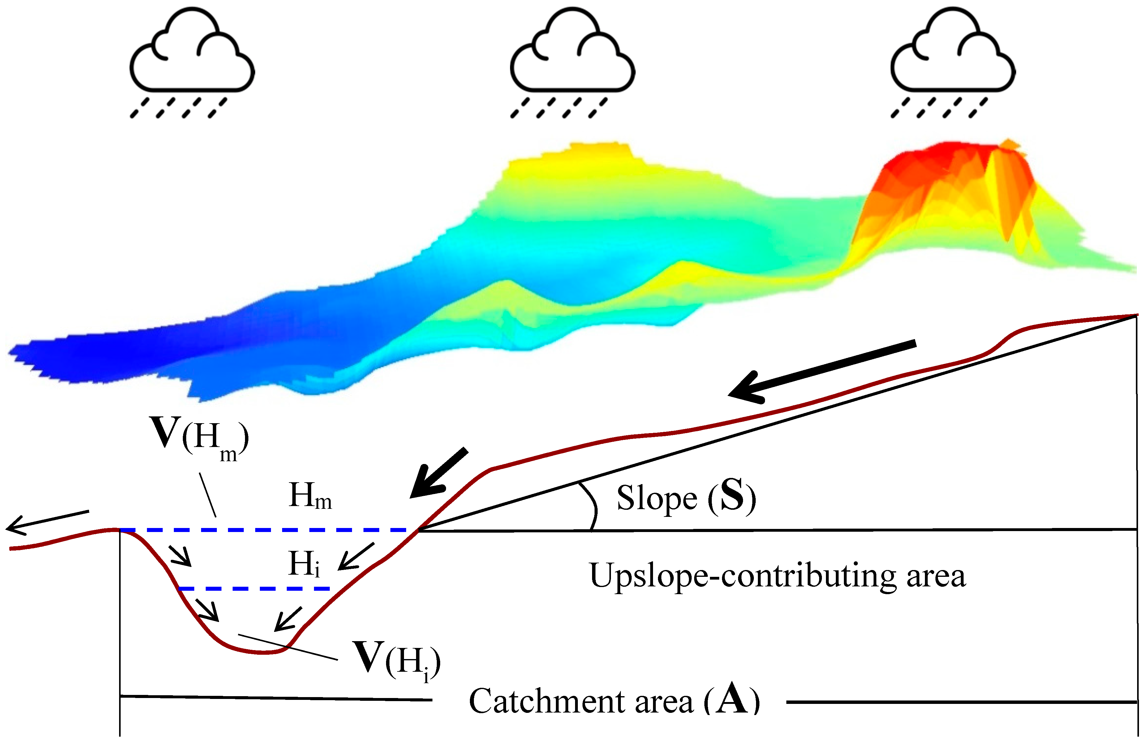
The profile of a typical topographic depression is given in Figure 1 to illustrate the conceptual framework of the Topographic Control Index.
As illustrated in Figure 1, topography plays a critical role in determining the direction and velocity of runoff, and also the potential places where pluvial flooding can occur. Given a specific study area, the catchments of depressions can be delineated using GIS analysis. Regarding a single depression, the more quickly it gets inundated, the more prone to flooding it is. The time required to fill a depression is affected by the topography in its catchment, such as the catchment area, the catchment slope, and the ponding volume of the depression. From a physically-based view, catchment area and catchment slope are inversely proportional to the time, while the ponding volume is proportional to the time. As a result, the TCI is defined as:
where A is the area of the catchment of the depression (m2), including the upslope-contributing area and the depression itself, S denotes the average slope (dimensionless) of the catchment, and V represents the ponding volume (m3) of the depression. The power of S is inspired by the Gauckler-Manning formula [44], in which S1/2 is linearly proportional to flow velocity. V is dependent on water depth Hi, and each depression has its own relationship between water depth and ponding volume, called the “depth-volume” relationship. The TCI is not dimensionless, and has a dimension of the natural log of m−1.
TCI = ln(A × S1/2/V)
Concerning the definition of the TCI, in which only the factors in connection with the topography are considered, it should be kept in mind that the TCI doesn’t reflect the actual risk of flooding, and thus, cannot take the place of the flooding risk. Nevertheless, TCI can act as a guide for urban planning, construction, and upgrading in terms of mitigating the risk of urban pluvial flooding. The TCI provides the spatial distribution and the proneness level of areas that have inherent disadvantages in drainage caused by topography; from there, it is possible to design proper measures for each area, like Low Impact Development, deep tunnels, pumps, and drainage pipe enlargements, to reduce runoff generation or increase the capacity of storage and conveying.
2.2. Calculation of TCI
Rivers are natural places to receive and transfer surface runoff. They have a much larger upstream contributing area than a single depression in an urban area, and the difference will be magnified due to the spatial connection of rivers. As a result, some depressions that are close to rivers will act as sub-depressions in a much larger depression, rather than single objects. However, complete inundation caused by pluvial flooding in a river catchment is very rare, whereas flooding in individual depressions in urban areas is more frequent [45]. Therefore, this study emphasizes a smaller spatial scale than a river catchment, and excludes rivers from the analysis.
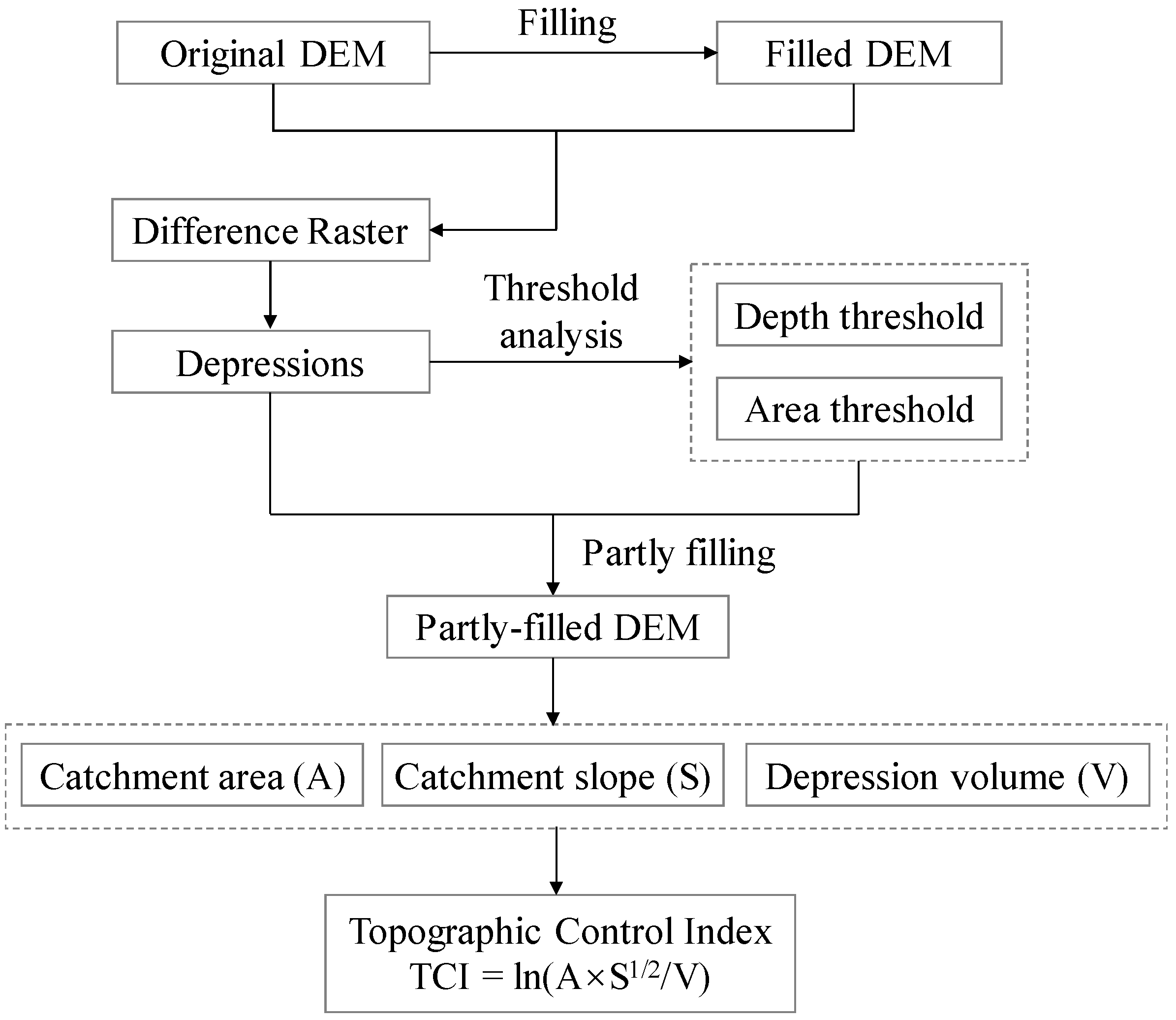
The workflow to calculate the TCI using a DEM without rivers is given in Figure 2. After identifying all depressions in the DEM, the thresholds of depth and area of depressions are derived. Then, the depressions that have a depth or an area less than the corresponding thresholds are filled. The partly-filled DEM is used to calculate the properties of the catchments of the remaining depressions, which are then employed to compute the Topographic Control Index for depressions.
2.2.1. Depression Locating
First, the original DEM is filled using GIS software, such as ArcGIS, SAGA GIS, or Whitebox, etc. Then, the depressions in the DEM can be located by simply subtracting the original DEM from the completely filled DEM and searching for non-zero cells in the derived difference raster. A group of non-zero cells that are spatially connected in the difference raster are considered to be one depression.
2.2.2. Depression Screening
(a) Area Threshold
Plenty of depressions exist in DEMs due to the micro-topography in urban environments, and also data noise. Noise may be introduced in the process of data acquisition or data resampling [46,47,48]. In order to reduce the impact of data noise, only depressions that have an area larger than 500 m2 are included in the analysis.
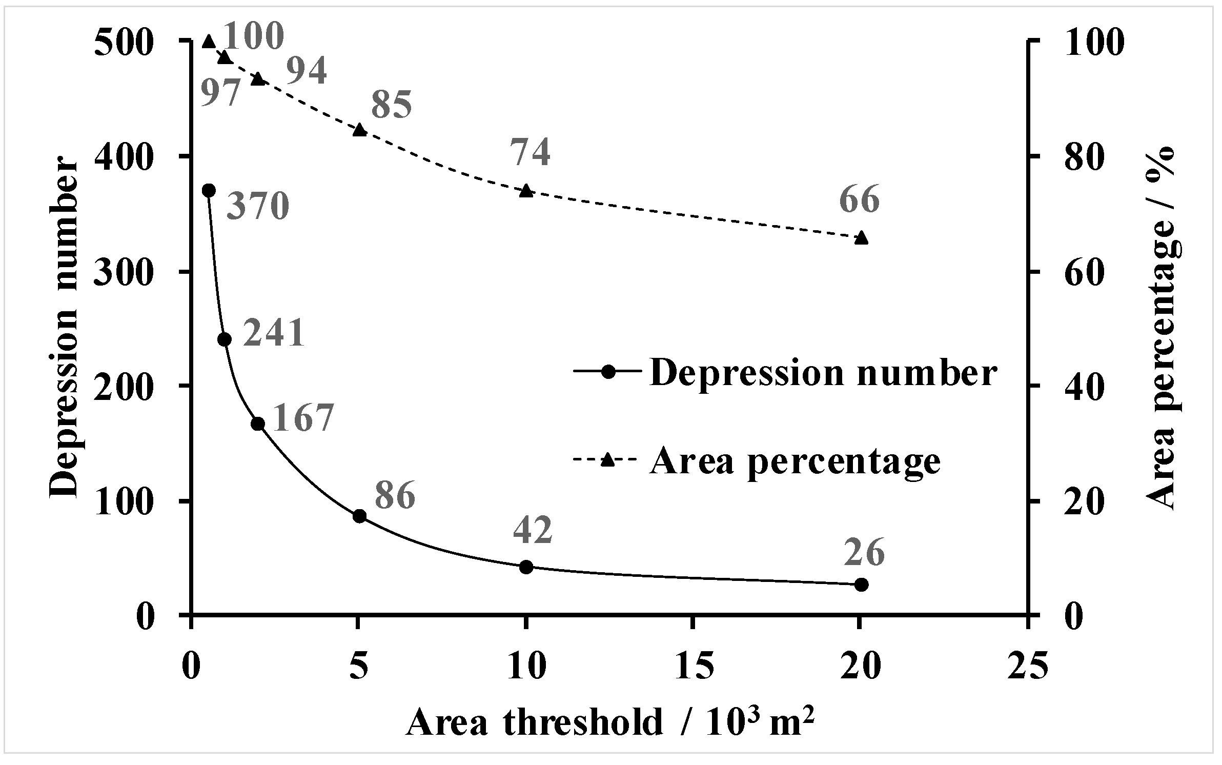
Flooding in large depressions causes more severe disruptions compared to small depressions, and thus, large depressions are the focus of the analysis. There is a general pattern like the pareto distribution in topography: a small number of depressions with large areas take a very large share in the total area of depressions [49]. This is also called the 80/20 rule. In view of this rule, a threshold in depression area can be found to strike a balance between the requirement of putting the focus on large depressions and the representativeness of the study. In this study, six thresholds, 500 m2, 1000 m2, 2000 m2, 5000 m2, 10,000 m2, and 20,000 m2, were tested. The number of depressions whose areas are larger than each threshold declines with the increase of the area threshold. The turning point on the area-number curve corresponds to the optimal area threshold. In addition, the area percentage that accounts for the depressions larger than the final area threshold should be above 80%, so that it can be representative of the study area.
(b) Depth Threshold
Water depth is a crucial indicator for flooding, in that its magnitude affects the degree of traffic chaos and property damage. Taking road traffic, for example, driving through a flooded area will put the engines and electronics in vehicles at risk of damage. The wading depth is frequently employed to measure the ability of vehicles to pass through flood water. Compared with other vehicles like Sport Utility Vehicles (SUVs) and pick-ups, cars are less able to pass through flood waters. So, the hazardous water depth in urban pluvial flooding is set according to the level of impact on cars. Car wading depths are subject to the height from the ground to the crucial level where sensitive electronics, air intake, and vulnerable areas are located; typical values are less than 30 cm. As a result, only depressions that have a maximum depth larger than 30 cm are included in the analysis.
Considering the uncertainties in DEMs, an empirical, 99th-percentile method is applied here to reduce the impact of outliers in elevation on computing the maximum depth of depressions. The depth of all cells within a depression are ranked in ascending order, and the 99th-percentile value is set as the maximum depth.
(c) Partly Filling
Depressions that have an area less than the area threshold or a maximum depth less than 30 cm are excluded from further analysis by filling. First, the original DEM is completely filled, and a difference raster is computed by subtracting the original DEM from the completely filled one. Then, in searching for a depression, a group of spatially-connected, non-zero cells in the difference raster, the properties of the depression, area and maximum depth, are calculated. If the area or the maximum depth of the depression is less than corresponding threshold, the elevation of the depression cells in the original DEM is replaced by the filled DEM. Otherwise, the elevation remains unchanged for the depression analysis. This procedure is repeated until all cells in the difference raster have been visited; the resulting raster is a partly-filled DEM. The properties of the remaining depressions are computed based on the partly-filled DEM.
2.2.3. Topographic Control Index (TCI)
(a) Catchment Area (A)
The area of a depression’s catchment equals the area of the depression plus its upslope-contributing area. Having identified the depressions, their upslope-contributing areas are needed to compute the catchment areas. It is common to search for upslope-contributing cells in a DEM by tracing in reverse with a routing algorithm, such as the D8 algorithm [50]. However, selecting appropriate flow routing algorithms in low-relief and flat areas is a problem, as discussed in the literature [50,51,52,53,54,55,56,57,58,59]. In this study, the elevation difference strategy [60] is employed because only the number of contributing cells, rather than flow paths, is required to calculate the upslope-contributing area. The contributing area is composed of all spatially-connected cells that are not lower than the depression.
(b) Catchment Slope (S)
In the calculation of the catchment slope, the part of the depression is not considered. It is assumed that surface runoff generated inside the depression immediately accumulates and does not need travel time. As a result, the catchment slope is represented by the average slope of the upslope-contributing area.
(c) Inundated Volume (V)
The “depth-volume” relationship of a depression can be obtained from a DEM using GIS spatial analysis. For a specific water depth, the elevation of its water surface equals the lowest elevation plus the water depth. Then, the corresponding volume can be calculated by adding the volumes of the cells, which are under the water surface within the depression. The “depth-volume” relationship is derived by repeating this procedure for different water depths. The volume for any water depth can easily be determined from this relationship. In this study, the target water depth is set as 30 cm, as mentioned in the analysis of depth threshold.
(d) TCI Map
After computing the properties of depressions, the TCI at a water depth of 30 cm for all depressions can be obtained using the Equation (1). Then, the spatial pattern of the topographic control is visualized by dividing the TCI values into three groups on the basis of the mean and standard deviation [61,62]: low (TCI ≤ mean), medium (mean < TCI ≤ mean + standard deviation), and high (TCI > mean + standard deviation).
2.3. Topographic Wetness Index (TWI)
TWI has been widely applied in hydrological processes, biological processes, vegetation patterns, and forests studies, and the assessment of flooding proneness [10,63]. The performance of TWI in representing the susceptibility to urban pluvial flooding was tested in its original form [8]:
where a is the local upslope area draining through a certain point per unit contour length, and b is the local slope in radians. TWI values are calculated using the SAGA GIS software (University of Hamburg, Hamburg, Germany. Available on www.saga-gis.org.). In this calculation, depression filling is a preliminary step, and the resulting TWI values are cell-based.
TWI = ln(a/tan b)
2.4. Impact of DEM Resolution
2.4.1. Topographic Representation
Applications using raster data need to strike a balance between computational efficiency and the precision of the representation, which are affected by the spatial resolution of DEM in contrasting ways. A generally employed strategy is to find a resolution which is as coarse as possible when the topographic representation is acceptable. The original 0.5 m-resolution DEM is resampled to resolutions of 1, 2, 5, and 10 m, and the best resampling resolution is determined by the patterns of two indicators, the number and total area of all depressions.
2.4.2. TCI Value
The impact of DEM resolution on a single depression is further investigated. The coarsening of DEM affects not only the area of a depression, but also its ponding volume and the area and average slope of its catchment. Subsequently, the TCI value of the depression changes accordingly.
The original 0.5 m-resolution DEM is resampled to resolutions of 1, 2, 5, and 10 m, and TCI calculation is repeated at each resolution. To measure the impact of DEM resolution on the TCI value of depressions, the results from the 0.5 m-resolution DEM are regarded as baseline, and the TCI deviation of a single depression within the resampled DEMs from its counterpart in the original DEM is computed. DEM resampling leads not only to the disappearance of depressions, but also to newly emerging depressions. The computation of TCI deviation and subsequent comparison require that each depression included in the analysis have a reference in the original DEM. However, newly-appearing depressions have no counterpart in the original DEM. As a result, this analysis only considered depressions that appear in both resampled DEMs and the original DEM. Then, the average deviation in TCI values of all the qualified depressions is employed to evaluate the effect of DEM resolution from an overall perspective. A more robust descriptor, median, is also given to reduce the impact of outliers in elevation.
2.5. Study Area
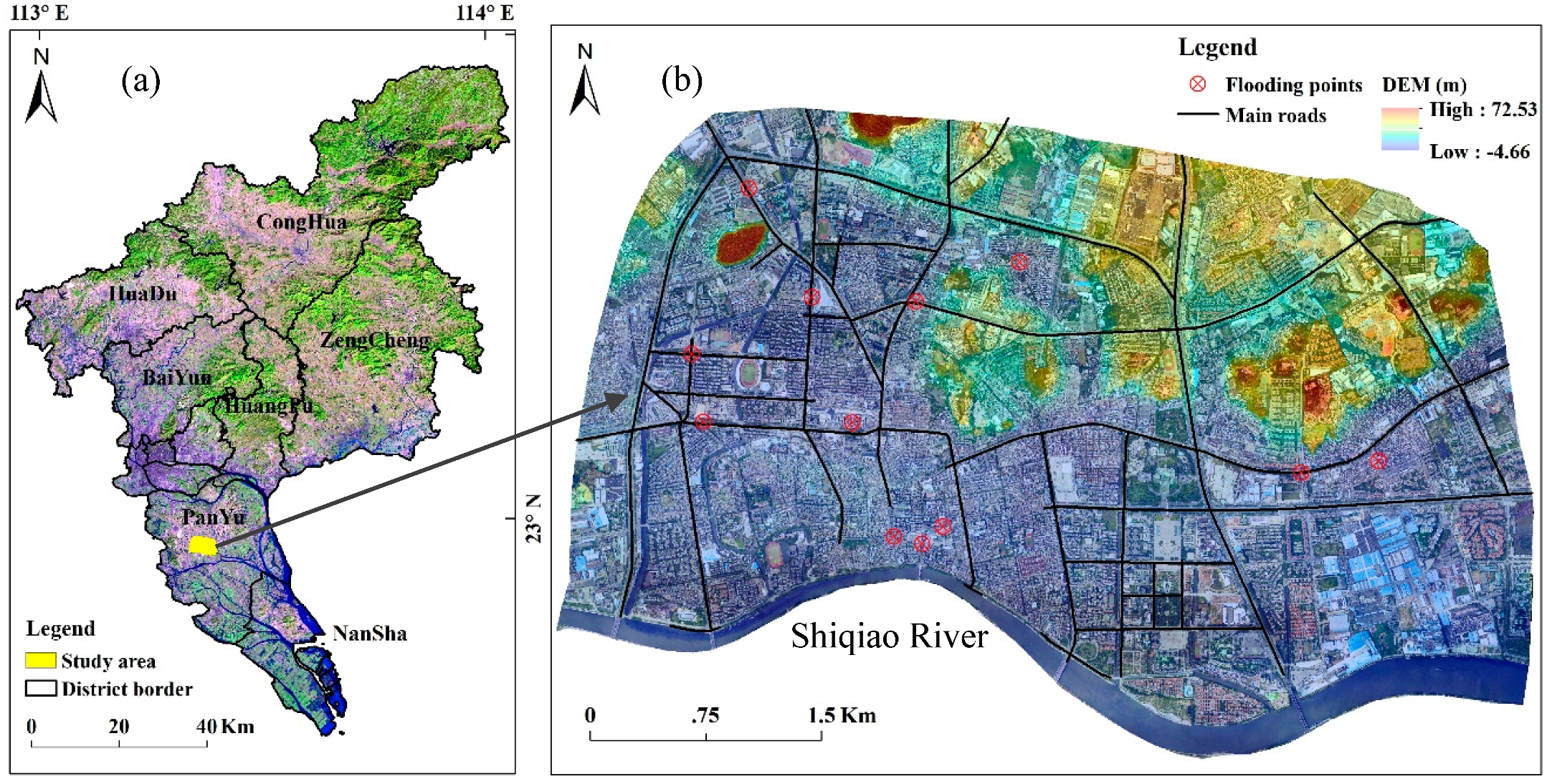
The study area is the downtown of Shiqiao, Panyu district, Guangzhou, China (Figure 3a), and has an area of 20.1 km2 and an annual rainfall of about 1800 mm [64]. The Shiqiao River runs through the downtown area from west to east in the south. Most creeks in the study area flow from north to south into the Shiqiao River (Figure 3b). A 0.5 m-resolution DEM was acquired by helicopter-based Light Detection and Ranging (LiDAR) equipment in 2014. Flooding points collected from newspaper reports and social media posts are employed as validation data for the results of TCI.
3. Results
3.1. Depressions
All depressions larger than the initial threshold, 500 m2, in the study area were identified. The number and area percentage of depressions that are larger than six thresholds—500, 1000, 2000, 5000, 10,000, and 20,000 m2—were then calculated, as shown in Figure 4. The turning point on the area-number curve stands at the threshold of 5000 m2, where 86 out of all 370 depressions possess 85% of the total area of depressions. The other depressions were filled before further analysis.
3.2. TCI Mapping and Validation
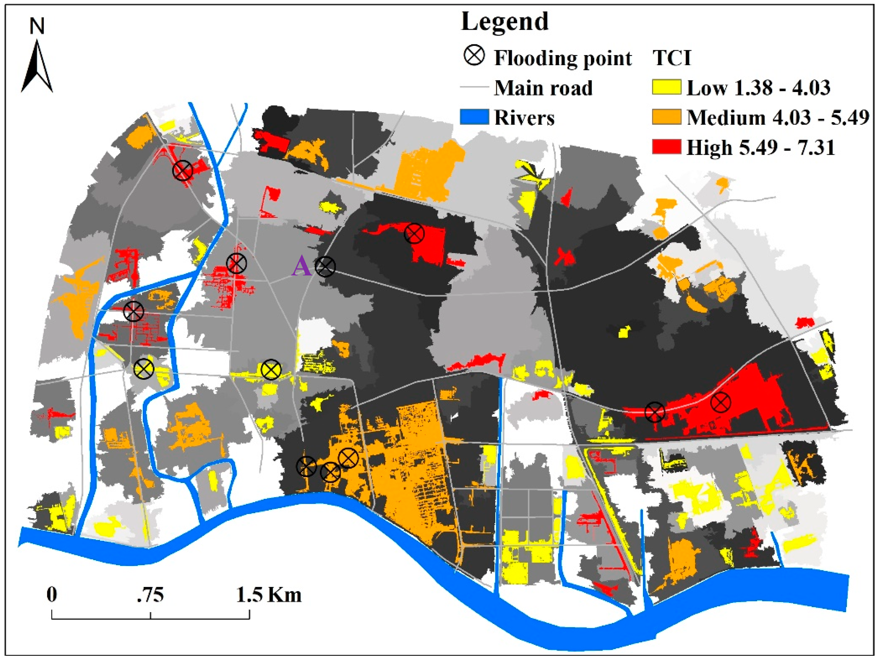
The spatial distribution of TCI at the water depth of 0.3 m was mapped in the study area (Figure 5). Twelve historical flooding points were collected from news reports and social media posts, and were shown to validate the TCI model. Most reported flooding points are located in places of high and median flooding susceptibility, indicating a good match between the results of the TCI model and flooding records. There is an exception for Point A, which is not within any depression. Actually, Point A does belong to a depression, but it was filled before the analysis because its depth is less than the threshold, i.e., 30 cm. In addition, there are still some depressions with large TCI values, but which are not reported. This suggests the potential of the TCI map to act as a guide for identifying flood-susceptible areas.
3.3. TWI Performance
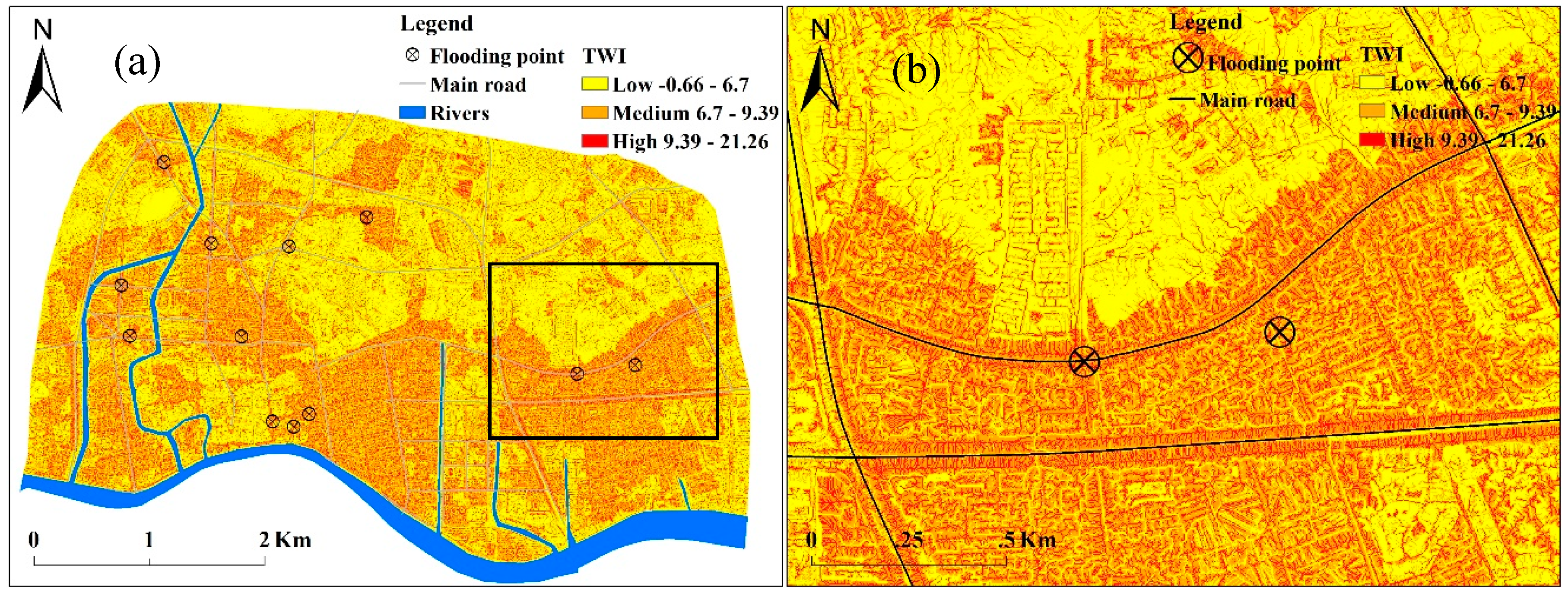
The TWI map is shown in Figure 6, in which TWI values were classified into three groups: low, medium, and high, using the same approach with the classification of TCI values. There is no clear pattern highlighting the area surrounding the flooding points from both global (Figure 6a) and local (Figure 6b) perspectives. To be specific, the flood-prone area is significantly overestimated by the TWI model. Therefore, it can be concluded that the depression-based TCI model did a better job in identifying potential regions with high flood susceptibility in urban areas in comparison with the cell-based TWI model.
3.4. Impact of DEM Resolution
3.4.1. Topographic Representation
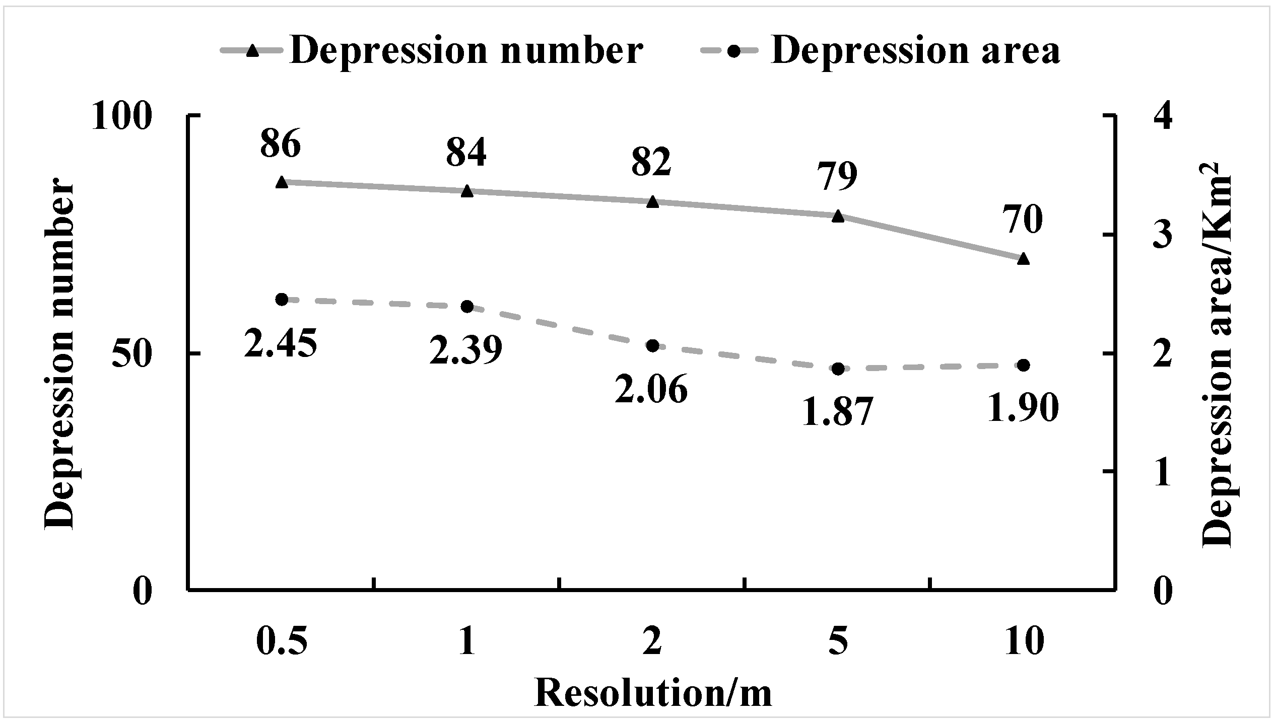
In the study area, the number and total area of depressions keep decreasing with increasing cell size (Figure 7), but at distinct rates. The number of depressions declines linearly from 0.5 m to 5 m, and has a large drop from 5 m to 10 m. The total area varies little from 0.5 m to 1 m and from 5 m to 10 m, but has a rapid decrease from 1 m through 5 m. This indicates that 1 m is the optimal resolution in terms of striking a balance between efficiency and precision.
3.4.2. TCI Value
Fifty-five depressions appeared in four resampled DEMs as well as the original DEM. The average and median of the TCI deviations at all resampled resolutions are listed in Table 1, and an obviously deteriorating pattern with increasing cell size can be observed. The performance of TCI at 1 and 2 m resolutions is significantly better than at 5 and 10 m.
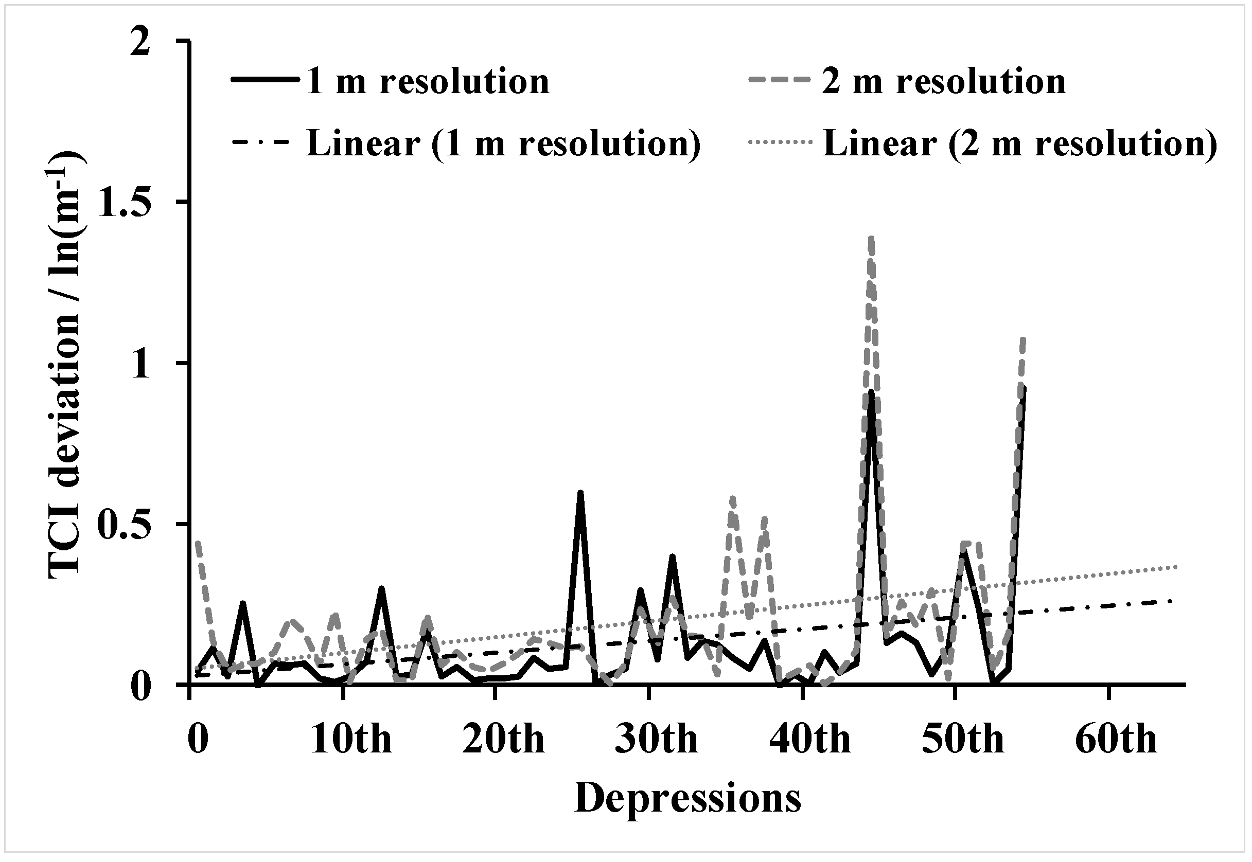
The possible connection between the depression area and the stability of the TCI value was further explored at resolutions of 1 and 2 m; the results are shown in Figure 8. All qualified 55 depressions were ranked by area in descending order. The first depression is the largest, and the last one is the smallest. Most of large deviations at both resolutions stand in the right half, and the linear patterns show that the level of uncertainty increases when the TCI model is applied to small depressions. The performance of the TCI model at 1 m resolution is slightly better than that at 2 m resolution.
To sum up, 1 m is the optimal resolution concerning topographical representation and computational efficiency. The performances of the TCI values at 1 and 2 m resolutions are significantly better than those at 5 and 10 m. The TCI values of large depressions are probably less affected by DEM coarsening, compared to small depressions.
4. Discussion
4.1. Applicability of TCI
In the development of urban pluvial flooding, topography is a necessary but insufficient condition. Pluvial flooding only occurs within depressions, and the actual flooding status of a single depression is subject to the interplay of other influential factors like rainfall, impervious surfaces, and the local drainage capacity. As a result, a TCI value making use of only topography cannot reflect the actual risk of flooding. Nevertheless, it can be widely applied in urban planning, construction, and upgrading in terms of mitigating flood risk because of the low requirement of input data and the increasing availability of high-resolution DEMs. The spatial distribution of TCI provides an operational guide for the design and maintenance of drainage facilities. A catchment with a high TCI value may need efficient measures to reduce runoff generation, detain excessive runoff, and enhance drainage capacity. Depressions deserve more attention, since runoff generated in these areas can’t be drained naturally, and needs extra assistance like pumps to overcome the effect of gravity.
Under extreme rainfall events which surpass the design criteria of urban drainage systems, the TCI is likely to be able to provide simple estimates of the flooding risk. The soil gets saturated quickly, and the original pervious surfaces turn into impervious ones. The spatial difference in runoff generation is quite limited, and thus, the topography along with rainfall dominate the formation of pluvial flooding.
4.2. Representation of Dynamic Process
Like other topographic indices, the TCI is also static, and thus, has difficulty representing the dynamics of storm water. It implicitly assumes that each depression is isolated and has its own contributing area. Actually, depressions with a small ponding volume can be inundated quickly during a heavy storm, and the runoff subsequently generated in their catchments spills out to a downstream depression. Typically, hydro-dynamic models are required to simulate the dynamic processes. Nevertheless, it is still possible for the TCI model to take into account this process to some extent by filling small depressions before the TCI computation. These filled depressions are then assigned as contributing areas of the remaining depressions in the DEM.
Regarding the influence of water level in the rivers, it is also beyond the capability of the TCI, and demands hydro-dynamic models to represent the interaction from a physically-based perspective.
4.3. Upper Limit of Depression Area
If the study area is large enough, it is possible to have huge depressions, for example, larger than 10 Km2. However, this kind of depression cannot get inundated completely only due to local storms. Consequently, a very large depression should be analyzed as a separate study area, rather than as a normal unit within the original study area. The upper limit of depression areas varies in different cities, and can be set according to historical records of flooding or empirical knowledge of the study area. In this study, the largest depression is 0.55 Km2, located in the middle bottom of the study area (Figure 5). Field investigation showed that most of this area suffers from frequent flooding; therefore, it was not considered as a standalone study area for the TCI analysis.
5. Conclusions
In order to quantify the role of topography in the development of urban pluvial flooding, this study proposes a new depression-base index, the Topographic Control Index. The TCI values for depressions can be computed by applying GIS analysis to a high-resolution DEM. A case study is tested using a 0.5 m-resolution LiDAR DEM in Guangzhou, China, and the derived TCI distribution matches with flooding records sufficiently, compared to the cell-based TWI map.
The impacts of DEM resolution on topographical representation and TCI values are also explored using the original 0.5 m resolution and four resampled resolutions, i.e., 1, 2, 5, and 10 m. The results show that (1) 1 m is the optimal resolution, i.e., that it strikes a balance between computational efficiency and representational precision, (2) TCI values at resolutions of 1 and 2 m are substantially more stable than those at the resolutions of 5 and 10 m, and (3) the level of uncertainty increases when the TCI model is applied to small depressions. Finally, it is recommended that a 1 m-resolution DEM be used for practical TCI applications, and that it not be used on small depressions.
With respect to the complexity of actual terrain, more case studies under distinct topographic conditions are required to improve our understanding of the role of topographic control in urban pluvial flooding.
Author Contributions
Conceptualization, H.H. and X.W. (Xianwei Wang); methodology, H.H. and X.C.; software, H.H.; validation, X.W. (Xina Wang); formal analysis, X.C. and L.L.; investigation, X.C.; resources, X.W. (Xina Wang); data curation, X.W. (Xina Wang); writing—original draft preparation, H.H.; writing—review and editing, H.H., X.C. and X.W. (Xianwei Wang); visualization, X.W. (Xina Wang); supervision, L.L.; project administration, H.H. and X.W. (Xianwei Wang); funding acquisition, L.L., H.H. and X.W. (Xianwei Wang).
Funding
This research was funded by the National Key Research and Development Program of China (#2018YFB0505500, #2018YFB0505502), the National Natural Science Foundation of China (#41301419, #41871085), the China Scholarship Council (#201806385016), and the Science and Technology Program of Guangzhou (#201707010098).
Acknowledgments
We thank the producer of the LiDAR DEM used in this study, Guangzhou Jiantong Surveying, Mapping and Geoinformation Technology Co., LTD.
Conflicts of Interest
The authors declare no conflict of interest. The funders had no role in the design of the study; in the collection, analyses, or interpretation of data; in the writing of the manuscript, or in the decision to publish the results.
References
- University of Maryland, Center for Disaster Resilience, and Texas A&M University, Galveston Campus, Center for Texas Beaches and Shores. The Growing Threat of Urban Flooding: A National Challenge; A. James Clark School of Engineering: College Park, MD, USA, 2018. [Google Scholar]
- Jang, J.H. An advanced method to apply multiple rainfall thresholds for urban flood warnings. Water 2015, 7, 6056–6078. [Google Scholar] [CrossRef]
- Zhang, H.; Cheng, J.; Wu, Z.; Li, C.; Qin, J.; Liu, T. Effects of impervious surface on the spatial distribution of urban waterlogging risk spots at multiple scales in Guangzhou, South China. Sustainability 2018, 10, 1589. [Google Scholar] [CrossRef]
- Yuan, Z.; Liang, C.; Li, D. Urban stormwater management based on an analysis of climate change: A case study of the Hebei and Guangdong provinces. Landsc. Urban Plan. 2018, 177, 217–226. [Google Scholar] [CrossRef]
- Huong, H.T.L.; Pathirana, A. Urbanization and climate change impacts on future urban flooding in Can Tho city, Vietnam. Hydrol. Earth Syst. Sci. 2013, 17, 379–394. [Google Scholar] [CrossRef] [Green Version]
- Mailhot, A.; Duchesne, S. Design criteria of urban drainage infrastructures under climate change. J. Water Resour. Plan. Manag. 2010, 136, 201–208. [Google Scholar] [CrossRef]
- Zhang, B.; Xie, G.D.; Li, N.; Wang, S. Effect of urban green space changes on the role of rainwater runoff reduction in Beijing, China. Landsc. Urban Plan. 2015, 140, 8–16. [Google Scholar] [CrossRef]
- Beven, K.J.; Kirkby, M.J. A physically based, variable contributing area model of basin hydrology. Hydrol. Sci. Bull. 1979, 24, 43–69. [Google Scholar] [CrossRef]
- Jalayer, F.; De Risi, R.; De Paola, F.; Giugni, M.; Manfredi, G.; Gasparini, P.; Topa, M.E.; Yonas, N.; Yeshitela, K.; Nebebe, A.; et al. Probabilistic GIS-based method for delineation of urban flooding risk hotspots. Nat. Hazards 2014, 73, 975–1001. [Google Scholar] [CrossRef]
- Pourali, S.H.; Arrowsmith, C.; Chrisman, N.; Matkan, A.A.; Mitchell, D. Topography Wetness Index Application in Flood-Risk-Based Land Use Planning. Appl. Spat. Anal. Policy 2016, 9, 39–54. [Google Scholar] [CrossRef]
- Manfreda, S.; Sole, A.; Fiorentino, M. Can the basin morphology alone provide an insight into floodplain delineation. Flood RecoveryInnov. Response 2008, 118, 47–56. [Google Scholar]
- Manfreda, S.; Di Leo, M.; Sole, A. Detection of Flood-Prone Areas Using Digital Elevation Models. J. Hydrol. Eng. 2011, 16, 781–790. [Google Scholar] [CrossRef]
- Hjerdt, K.N.; McDonnell, J.J.; Seibert, J.; Rodhe, A. A new topographic index to quantify downslope controls on local drainage. Water Resour. Res. 2004, 40, W056021–W056026. [Google Scholar] [CrossRef]
- Rennó, C.D.; Nobre, A.D.; Cuartas, L.A.; Soares, J.V.; Hodnett, M.G.; Tomasella, J.; Waterloo, M.J. HAND, a new terrain descriptor using SRTM-DEM: Mapping terra-firme rainforest environments in Amazonia. Remote Sens. Environ. 2008, 112, 3469–3481. [Google Scholar] [CrossRef]
- Jafarzadegan, K.; Merwade, V.; Saksena, S. A geomorphic approach to 100-year floodplain mapping for the Conterminous United States. J. Hydrol. 2018, 561, 43–58. [Google Scholar] [CrossRef]
- Brunner, G.W. HEC-RAS, River Analysis System Hydraulic Reference Manual; Version 5.0; US Army Corps of Engineers Hydrologic Engineering Center: Davis, CA, USA, 2016. [Google Scholar]
- Bates, P.D.; De Roo, A.P.J. A simple raster-based model for flood inundation simulation. J. Hydrol. 2000, 236, 54–77. [Google Scholar] [CrossRef]
- Yu, D.; Lane, S.N. Urban fluvial flood modelling using a two-dimensional diffusion-wave treatment, part 1, Mesh resolution effects. Hydrol. Process. 2006, 20, 1541–1565. [Google Scholar] [CrossRef]
- Yu, D.; Lane, S.N. Urban fluvial flood modelling using a two-dimensional diffusion-wave treatment, part 2, Development of a sub-grid-scale treatment. Hydrol. Process. 2006, 20, 1567–1583. [Google Scholar] [CrossRef]
- Liu, L.; Liu, Y.; Wang, X.; Yu, D.; Liu, K.; Huang, H.; Hu, G. Developing an effective 2-D urban flood inundation model for city emergency management based on cellular automata. Nat. Hazards Earth Syst. Sci. 2015, 15, 381–391. [Google Scholar] [CrossRef] [Green Version]
- Ernst, J.; Dewals, B.J.; Detrembleur, S.; Archambeau, P.; Erpicum, S.; Pirotton, M. Micro-scale flood risk analysis based on detailed 2D hydraulic modelling and high resolution geographic data. Nat. Hazards 2010, 55, 181–209. [Google Scholar] [CrossRef]
- Mustafa, A.; Bruwier, M.; Archambeau, P.; Erpicum, S.; Pirotton, M.; Dewals, B.; Teller, J. Effects of spatial planning on future flood risks in urban environments. J. Environ. Manag. 2018, 225, 193–204. [Google Scholar] [CrossRef]
- Samela, C.; Troy, T.J.; Manfreda, S. Geomorphic classifiers for flood-prone areas delineation for data-scarce environments. Adv. Water Resour. 2017, 102, 13–28. [Google Scholar] [CrossRef]
- Clubb, F.J.; Mudd, S.M.; Milodowski, D.T.; Valters, D.A.; Slater, L.J.; Hurst, M.D.; Limaye, A.B. Geomorphometric delineation of floodplains and terraces from objectively defined topographic thresholds. Earth Surf. Dyn. 2017, 5, 369–385. [Google Scholar] [CrossRef] [Green Version]
- De Risi, R.; Jalayer, F.; De Paola, F.; Lindley, S. Delineation of flooding risk hotspots based on digital elevation model, calculated and historical flooding extents: The case of Ouagadougou. Stoch. Environ. Res. Risk Assess. 2018, 32, 1545–1559. [Google Scholar] [CrossRef]
- Jafarzadegan, K.; Merwade, V. A DEM-based approach for large-scale floodplain mapping in ungauged watersheds. J. Hydrol. 2017, 550, 650–662. [Google Scholar] [CrossRef]
- Try, S.; Lee, G.; Yu, W.; Oeurng, C. Delineation of flood-prone areas using geomorphological approach in the Mekong River Basin. Quat. Int. 2019, 503, 79–86. [Google Scholar] [CrossRef]
- Chapi, K.; Singh, V.P.; Shirzadi, A.; Shahabi, H.; Bui, D.T.; Pham, B.T.; Khosravi, K. A novel hybrid artificial intelligence approach for flood susceptibility assessment. Environ. Model. Softw. 2017, 95, 229–245. [Google Scholar] [CrossRef]
- Gnecco, G.; Morisi, R.; Roth, G.; Sanguineti, M.; Taramasso, A.C. Supervised and semi-supervised classifiers for the detection of flood-prone areas. Soft Comput. 2017, 21, 3673–3685. [Google Scholar] [CrossRef]
- Xu, H.; Ma, C.; Lian, J.; Xu, K.; Chaima, E. Urban flooding risk assessment based on an integrated k-means cluster algorithm and improved entropy weight method in the region of Haikou, China. J. Hydrol. 2018, 563, 975–986. [Google Scholar] [CrossRef]
- Hong, H.; Tsangaratos, P.; Ilia, I.; Liu, J.; Zhu, A.X.; Chen, W. Application of fuzzy weight of evidence and data mining techniques in construction of flood susceptibility map of Poyang County, China. Sci. Total Environ. 2018, 625, 575–588. [Google Scholar] [CrossRef]
- Khosravi, K.; Pham, B.T.; Chapi, K.; Shirzadi, A.; Shahabi, H.; Revhaug, I.; Prakash, I.; Tien Bui, D. A comparative assessment of decision trees algorithms for flash flood susceptibility modeling at Haraz watershed, northern Iran. Sci. Total Environ. 2018, 627, 744–755. [Google Scholar] [CrossRef]
- Giovannettone, J.; Copenhaver, T.; Burns, M.; Choquette, S. A Statistical Approach to Mapping Flood Susceptibility in the Lower Connecticut River Valley Region. Water Resour. Res. 2018, 54, 7603–7618. [Google Scholar] [CrossRef]
- Ma, M.; Liu, C.; Zhao, G.; Xie, H.; Jia, P.; Wang, D.; Wang, H.; Hong, Y. Flash flood risk analysis based on machine learning techniques in the Yunnan Province, China. Remote Sens. 2019, 11, 170. [Google Scholar] [CrossRef]
- Woznicki, S.A.; Baynes, J.; Panlasigui, S.; Mehaffey, M.; Neale, A. Development of a spatially complete floodplain map of the conterminous United States using random forest. Sci. Total Environ. 2019, 647, 942–953. [Google Scholar] [CrossRef] [PubMed]
- Drǎgut, L.; Eisank, C.; Strasser, T. Local variance for multi-scale analysis in geomorphometry. Geomorphology 2011, 130, 162–172. [Google Scholar] [CrossRef] [PubMed] [Green Version]
- Gillin, C.P.; Bailey, S.W.; McGuire, K.J.; Prisley, S.P. Evaluation of lidar-derived DEMs through terrain analysis and field comparison. Photogramm. Eng. Remote Sens. 2015, 81, 387–396. [Google Scholar] [CrossRef]
- Le Roy, S.; Pedreros, R.; André, C.; Paris, F.; Lecacheux, S.; Marche, F.; Vinchon, C. Coastal flooding of urban areas by overtopping: Dynamic modelling application to the Johanna storm (2008) in Gâvres (France). Nat. Hazards Earth Syst. Sci. 2015, 15, 2497–2510. [Google Scholar] [CrossRef]
- Winters, B.A.; Angel, J.; Ballerine, C.; Byard, J.; Flegel, A.; Gambill, D.; Jenkins, E.; McConkey, S.; Markus, M.; Bender, B.A.; et al. Report for the Urban Flooding Awareness Act; Illinois Department of Natural Resources: Springfield, IL, USA, 2015. [Google Scholar]
- Huang, H.; Chen, X.; Zhu, Z.; Xie, Y.; Liu, L.; Wang, X.; Wang, X.; Liu, K. The changing pattern of urban flooding in Guangzhou, China. Sci. Total Environ. 2018, 622–623, 394–401. [Google Scholar] [CrossRef]
- Di Salvo, C.; Ciotoli, G.; Pennica, F.; Cavinato, G.P. Pluvial flood hazard in the city of Rome (Italy). J. Maps 2017, 13, 545–553. [Google Scholar] [CrossRef] [Green Version]
- Jamali, B.; Löwe, R.; Bach, P.M.; Urich, C.; Arnbjerg-Nielsen, K.; Deletic, A. A rapid urban flood inundation and damage assessment model. J. Hydrol. 2018, 564, 1085–1098. [Google Scholar] [CrossRef]
- Jamali, B.; Bach, P.M.; Cunningham, L.; Deletic, A. A Cellular Automata Fast Flood Evaluation (CA-ffé) Model. Water Resour. Res. 2019, 55, 4936–4953. [Google Scholar] [CrossRef]
- Manning, R. On the flow of water in open channels and pipes. Trans. Inst. Civ. Eng. Irel. 1891, 20, 161–207. [Google Scholar]
- Cherqui, F.; Belmeziti, A.; Granger, D.; Sourdril, A.; Le Gauffre, P. Assessing urban potential flooding risk and identifying effective risk-reduction measures. Sci. Total Environ. 2015, 514, 418–425. [Google Scholar] [CrossRef] [PubMed]
- Lindsay, J.B.; Francioni, A.; Cockburn, J.M.H. LiDAR DEM smoothing and the preservation of drainage features. Remote Sens. 2019, 11, 1926. [Google Scholar] [CrossRef]
- Sanders, B.F. Evaluation of on-line DEMs for flood inundation modeling. Adv. Water Resour. 2007, 30, 1831–1843. [Google Scholar] [CrossRef]
- Shi, W.; Deng, S.; Xu, W. Extraction of multi-scale landslide morphological features based on local Gi* using airborne LiDAR-derived DEM. Geomorphology 2018, 303, 229–242. [Google Scholar] [CrossRef]
- Bertassello, L.E.; Rao, P.S.C.; Jawitz, J.W.; Botter, G.; Le, P.V.V.; Kumar, P.; Aubeneau, A.F. Wetlandscape Fractal Topography. Geophys. Res. Lett. 2018, 45, 6983–6991. [Google Scholar] [CrossRef] [Green Version]
- O’Callaghan, J.F.; Mark, D.M. The extraction of drainage networks from digital elevation data. Comput. Vis. Graph. Image Process. 1984, 28, 323–344. [Google Scholar] [CrossRef]
- Jenson, S.K.; Domingue, J.O. Extracting topographic structure from digital elevation data for geographic information system analysis. Photogramm. Eng. Remote Sens. 1988, 54, 1593–1600. [Google Scholar]
- Freeman, T.G. Calculating catchment area with divergent flow based on a regular grid. Comput. Geosci. 1991, 17, 413–422. [Google Scholar] [CrossRef]
- Fairfield, J.; Leymarie, P. Drainage networks from grid digital elevation models. Water Resour. Res. 1991, 27, 709–717. [Google Scholar] [CrossRef]
- Costa Cabral, M.C.; Burges, S.J. Digital Elevation Model Networks (DEMON): A model of flow over hillslopes for computation of contributing and dispersal areas. Water Resour. Res. 1994, 30, 1681–1692. [Google Scholar] [CrossRef]
- Quinn, P.F.; Beven, K.J.; Lamb, R. The in(a/tan/β) index: How to calculate it and how to use it within the topmodel framework. Hydrol. Process. 1995, 9, 161–182. [Google Scholar] [CrossRef]
- Tarboton, D.G. A new method for the determination of flow directions and upslope areas in grid digital elevation models. Water Resour. Res. 1997, 33, 309–319. [Google Scholar] [CrossRef] [Green Version]
- Wilson, J.P.; Aggett, G.; Deng, Y.; Lam, C.S. Water in the Landscape: A Review of Contemporary Flow Routing Algorithms; Springer: Berlin/Heidelberg, Germany, 2008; pp. 213–236. [Google Scholar]
- Wilson, J.P. Digital terrain modeling. Geomorphology 2012, 137, 107–121. [Google Scholar] [CrossRef]
- Woodrow, K.; Lindsay, J.B.; Berg, A.A. Evaluating DEM conditioning techniques, elevation source data, and grid resolution for field-scale hydrological parameter extraction. J. Hydrol. 2016, 540, 1022–1029. [Google Scholar] [CrossRef]
- Wang, L.; Liu, H. An efficient method for identifying and filling surface depressions in digital elevation models for hydrologic analysis and modelling. Int. J. Geogr. Inf. Sci. 2006, 20, 193–213. [Google Scholar] [CrossRef]
- Ayalew, L.; Yamagishi, H. The application of GIS-based logistic regression for landslide susceptibility mapping in the Kakuda-Yahiko Mountains, Central Japan. Geomorphology 2005, 65, 15–31. [Google Scholar] [CrossRef]
- Wang, Y.; Li, Z.; Tang, Z.; Zeng, G. A GIS-Based Spatial Multi-Criteria Approach for Flood Risk Assessment in the Dongting Lake Region, Hunan, Central China. Water Resour. Manag. 2011, 25, 3465–3484. [Google Scholar] [CrossRef]
- Sørensen, R.; Zinko, U.; Seibert, J. On the calculation of the topographic wetness index: Evaluation of different methods based on field observations. Hydrol. Earth Syst. Sci. 2006, 10, 101–112. [Google Scholar] [CrossRef]
- Yang, L.; Scheffran, J.; Qin, H.; You, Q. Climate-related flood risks and urban responses in the Pearl River Delta, China. Reg. Environ. Chang. 2014, 15, 379–391. [Google Scholar] [CrossRef]
Figure 1.
Profile of a typical topographic depression. The area embraced by the upper horizontal dashed blue line and the land surface is a depression. Hm is the maximum water depth in the depression when it is completely inundated, and Hi is any depth smaller than Hm. V(Hm) and V(Hi) are the maximum ponding volume and the volume at the depth Hi, respectively. The flow directions of the surface runoff are represented by arrows; thicker ones denote runoff from the upslope-contributing area of the depression.

Figure 2.
The workflow to derive the Topographic Control Index for depressions.

Figure 3.
The study area in Guangzhou, China: location (a), and topography, main roads, and historical flooding points (b).
Figure 3.
The study area in Guangzhou, China: location (a), and topography, main roads, and historical flooding points (b).

Figure 4.
The changes in the number and area percentage of depressions at area thresholds of 500, 1000, 2000, 5000, 10,000, and 20,000 m2. The area percentage is 100 when the area threshold is 500 m2.
Figure 4.
The changes in the number and area percentage of depressions at area thresholds of 500, 1000, 2000, 5000, 10,000, and 20,000 m2. The area percentage is 100 when the area threshold is 500 m2.

Figure 5.
TCI (ln(m−1)) map derived from the original 0.5 m-resolution LiDAR DEM at the water depth 0.3 m. TCI values were divided into three groups: Low (yellow, TCI ≤ mean), Medium (orange, mean < TCI ≤ mean + standard deviation), and High (red, TCI > mean + standard deviation).
Figure 5.
TCI (ln(m−1)) map derived from the original 0.5 m-resolution LiDAR DEM at the water depth 0.3 m. TCI values were divided into three groups: Low (yellow, TCI ≤ mean), Medium (orange, mean < TCI ≤ mean + standard deviation), and High (red, TCI > mean + standard deviation).

Figure 6.
The spatial distribution of TWI in the study area (a), and the part in the rectangle (b) that has two flooding points. TWI values are divided into three groups: Low (yellow, TWI ≤ mean), Medium (orange, mean < TWI ≤ mean + standard deviation), and High (red, TWI > mean + standard deviation).

Figure 7.
Changes in the number and total area of depressions with increasing DEM cell size.

Figure 8.
The pattern of TCI deviations of depressions at resolutions of 1 and 2 m. All 55 qualified depressions are ranked by area in descending order. ‘Linear’ in the legend means the linear trend of TCI values.
Figure 8.
The pattern of TCI deviations of depressions at resolutions of 1 and 2 m. All 55 qualified depressions are ranked by area in descending order. ‘Linear’ in the legend means the linear trend of TCI values.


Table 1.
Average and median of TCI deviations at four resampled resolutions.
| Resolution/m | 1 | 2 | 5 | 10 |
|---|---|---|---|---|
| Average/ln(m−1) | 0.131 | 0.187 | 0.446 | 0.781 |
| Median/ln(m−1) | 0.065 | 0.122 | 0.351 | 0.687 |
© 2019 by the authors. Licensee MDPI, Basel, Switzerland. This article is an open access article distributed under the terms and conditions of the Creative Commons Attribution (CC BY) license (http://creativecommons.org/licenses/by/4.0/).
Share and Cite
MDPI and ACS Style
Huang, H.; Chen, X.; Wang, X.; Wang, X.; Liu, L. A Depression-Based Index to Represent Topographic Control in Urban Pluvial Flooding. Water 2019, 11, 2115. https://doi.org/10.3390/w11102115
AMA Style
Huang H, Chen X, Wang X, Wang X, Liu L. A Depression-Based Index to Represent Topographic Control in Urban Pluvial Flooding. Water. 2019; 11(10):2115. https://doi.org/10.3390/w11102115
Chicago/Turabian StyleHuang, Huabing, Xi Chen, Xianwei Wang, Xina Wang, and Lin Liu. 2019. "A Depression-Based Index to Represent Topographic Control in Urban Pluvial Flooding" Water 11, no. 10: 2115. https://doi.org/10.3390/w11102115
Note that from the first issue of 2016, this journal uses article numbers instead of page numbers. See further details here.