Spatiotemporal Evolution of Droughts and Their Teleconnections with Large-Scale Climate Indices over Guizhou Province in Southwest China


1
State Key Laboratory of Hydrology-Water Resources and Hydraulic Engineering, Hohai University, Nanjing 210098, China
2
College of Hydrology and Water Resources, Hohai University, Nanjing 210098, China
3
School of Hydraulic and Ecological Engineering, Nanchang Institute of Technology, Nanchang 330099, China
4
Institute of Surface-Earth System Science, Tianjin University, Tianjin 300072, China
*
Author to whom correspondence should be addressed.
Water 2019, 11(10), 2104; https://doi.org/10.3390/w11102104
Submission received: 14 August 2019
/
Revised: 26 September 2019
/
Accepted: 4 October 2019
/
Published: 10 October 2019
(This article belongs to the Section Hydrology)
Abstract
:The spatiotemporal evolution of meteorological droughts in Guizhou Province, Southwest China is analyzed based on a new set of the Standardized Precipitation Index series that mainly includes drought events that occurred from 1961 to 2004 at 81 meteorological stations. The cluster analysis shows that the study region can be classified into six homogeneous sub-regions where the drought characteristics and their temporal evolutions are quite different. The trend test and periodicity analysis indicate that Guizhou Province experienced a drier trend, which was most significant in the western parts of the region. It was found that the intensified drought severity was not always coincident with the drier trend but relied on the occurrence of extreme drought events. The trends of drier climate and drought severity were highly coincident with the temporal evolution of the drought periodicities, which were shortened from 1–4 years to less than one year. The shortened drought periodicity was found to be associated principally with a shift of the large-scale dominant climate indices from the North Atlantic Oscillation to the Indian Ocean Dipole after the late 1970s, and variations of the extreme drought events were mostly related to NINO34 in the study region.
1. Introduction
Drought is often represented in terms of drought indices, such as the Standardized Precipitation Index (SPI), the Standardized Precipitation Evapotranspiration Index (SPEI) [1], the Palmer Drought Severity Index (PDSI) [2], and the Surface Water Supply Index (SWSI) [3]. The drought indices can be characterized by attributes such as duration, spatial extent, and intensity [4]. Since drought emerges in space and time, many studies focused on the temporal (one-dimensional) evolution of droughts in a specific area (e.g., [5]), and the spatial (two-dimensional) structure of drought patterns in a fixed time scale (e.g., [6,7]). In recent years, three-dimensional approaches have been developed in order to represent true drought evolutions of the spatiotemporal coherence [8,9,10,11], such as the severity–area–duration (SAD) relationship that jointly represents drought characterization in space and time in higher dimensions [12].
The three-dimensional method requires complex computation steps, such as locating neighboring cells that meet drought conditions [8] and defining criteria that have to be met for a space–time region to be considered a drought event [9,10]. Moreover, the identified spatial extend of droughts is often discontinuous in time. From aspects of agriculture and water supply management, choosing regions of drought a priori is helpful for optimizing water resources and developing effective mitigation strategies. For example, for the purpose of providing more robust integrated water management insights under the implementation of the European Water Framework Directive, drought assessment was suggested on the basis of the basin-scale approach and information [13]. Since hydro-metrological conditions used for drought evaluations are based on at-site observations, simply using the mean of at-site drought characteristics to represent basin-scale droughts would reduce drought severity due to the strong asynchronous evolutions of droughts at sites in a large basin [14]. Therefore, it is necessary to divide a heterogeneous region into several homogeneous sub-regions. In each of the homogenous sub-regions, temporal evolutions of at-site drought characteristics should present similar behavior. Consequently, the mean of at-site drought series in each of the homogeneous sub-regions can be used to quantify temporal drought evolutions of sub-regional drought characteristics and integration of temporal drought evolutions in all the sub-regions could alternatively represent the spatiotemporal evolutions of droughts in a region.
A variety of techniques exist for the extraction of homogeneous sub-regions from at-site or grid data, e.g., principal component analysis (PCA) based on the empirical orthogonal function (EOF) analysis or the rotated empirical orthogonal function (REOF) [15], as well as cluster analysis (CA) [16]. Among the clustering techniques, hierarchical clustering and partitioning clustering are two main approaches in time series clustering algorithms [17], popularly applied to group the similar sites into a homogeneous sub-region based on at-site SPI time series [16,18]. In these approaches, the selection of an appropriate series at sites with similar temporal variability is vital for isolating sub-regions. Since the drought is usually defined by the departure of climate and hydrological variables from the ‘‘normal’’ or average amount (e.g., SPI ≤ −1 in Table 1), statistical identification of homogeneous regions using an entire SPI series may mask the similarity of drought events if the non-drought events (e.g., SPI > −1 in Table 1) between sites are more similar than the drought events in the series. Therefore, it is necessary to select a set of representative SPI series that ensure concurrence of the drought events at all sites.
Spatial and temporal evolution of droughts is caused by climate anomalies, particularly, extreme climate events, and the heterogeneity of the landscape. Frequent severe and sustained droughts have hit Southwest China in the last decade. For example, from autumn 2009 to spring 2010, a prolonged drought occurred over large areas of Southwest China. Guizhou Province is located in one of the most severe and extreme drought cluster areas [19] of Southwest China. The extreme and severe drought experienced in this province is because of special atmospheric circulation in Eastern Asia and the unique topography. Previous studies have documented that precipitation and drought variability are significantly linked to large-scale climate oscillations in Southwest China [20,21,22]. For example, Feng et al. [20] pointed out that droughts in Southwest China during the dry season are, in general, consistent with local anomalous descent in the middle troposphere, associated with sea surface temperature (SST) anomalies in the North Atlantic and Hadley circulation. Zhang et al. [23] and Wang et al. [21] found that the autumn precipitation over Southwest China reduced due to warm SST anomalies in the Western North Pacific and tropical Northwest Pacific, while Huang et al. [24] found that below-normal spring precipitation over Southwest China may be associated with warm SST anomalies in the Indian Ocean. The El Niño Southern Oscillation (ENSO), as a coupled ocean–atmosphere tropical Pacific phenomenon, also displays a remarkable influence on precipitation and droughts over Southwest China (e.g., [20,22]). Specifically, high mountains and special karst landscapes lead to extremely uneven distribution of precipitation and available water resources in Guizhou Province of China.
Until now, there have been many studies on drought evolutions based on the drought indices such as SPI, RDI (Reconnaissance Drought Index), and SPEI (the Standardized Precipitation Evapotranspiration Index) over the Guizhou Province and Southwest China [25,26,27,28,29]. Most analyses show a drying trend in the region. For example, Yang et al. [26] developed a multi-scale SPI to identify extreme severe drought events in China between 1961 and 2010 and found that Southwest China demonstrated the most extreme droughts clusters, compared with other regions of China. Li et al. [27] applied the SPEI to analyze drought trends and found a drying trend in Southwestern China. In Guizhou Province, Feng et al. [28], Chen et al. [29], and Cheng et al. [25] analyzed spatial and temporal characteristics of droughts using at-site SPI, SPEI, and three drought indices of SPI, CI (the Comprehensive Meteorological Drought Index), and RDI, respectively. Feng et al. [28] found that SPI decreased in spring and autumn, Chen et al. [29] detected that SPEI decreased at annual, spring, summer, and autumn scales, and Cheng et al. [25] detected that three drought indices decreased at annual and autumn scales. These drying trends are obtained from a large-scale analysis of the SPI index or sparse observation stations (e.g., 19 stations by Cheng et al. [25] and Chen et al. [29] and nine stations by Feng et al. [28]). Thus, these studies cannot fully capture the spatial characteristics of the temporal drought evolutions, such as sub-regional droughts. Moreover, they seldom simultaneously analyzed the spatiotemporal coherence of the drought indices with drought severity characteristics, as well as with driving causes of climate anomaly, such as teleconnections with large-scale climate oscillations.
The objective of the study is to fully describe the spatiotemporal evaluations of droughts and their association with large-scale climate oscillations in Guizhou Province of Southwest China. Specifically, the study is focused on how the at-site SPI series can be grouped into several sub-regions, each of which includes at-site SPI series with a similar drought characteristic, how the sub-regional drought characteristics change with space and time, and whether the drought changes are associated with large-scale climate oscillations. First, a new set of at-site SPI series that mostly consists of drought events between 1961 and 2004 at 81 meteorological stations was developed. Then, the new set of at-site SPI series was applied to identify homogeneous sub-regions by the cluster analysis method. The spatiotemporal evolutions of droughts include trend, periodicity, and teleconnection with large-scale climate indices, are detected by the Mann–Kendall method, wavelet analysis, and the wavelet coherence analysis, respectively.
2. Study Area and Data
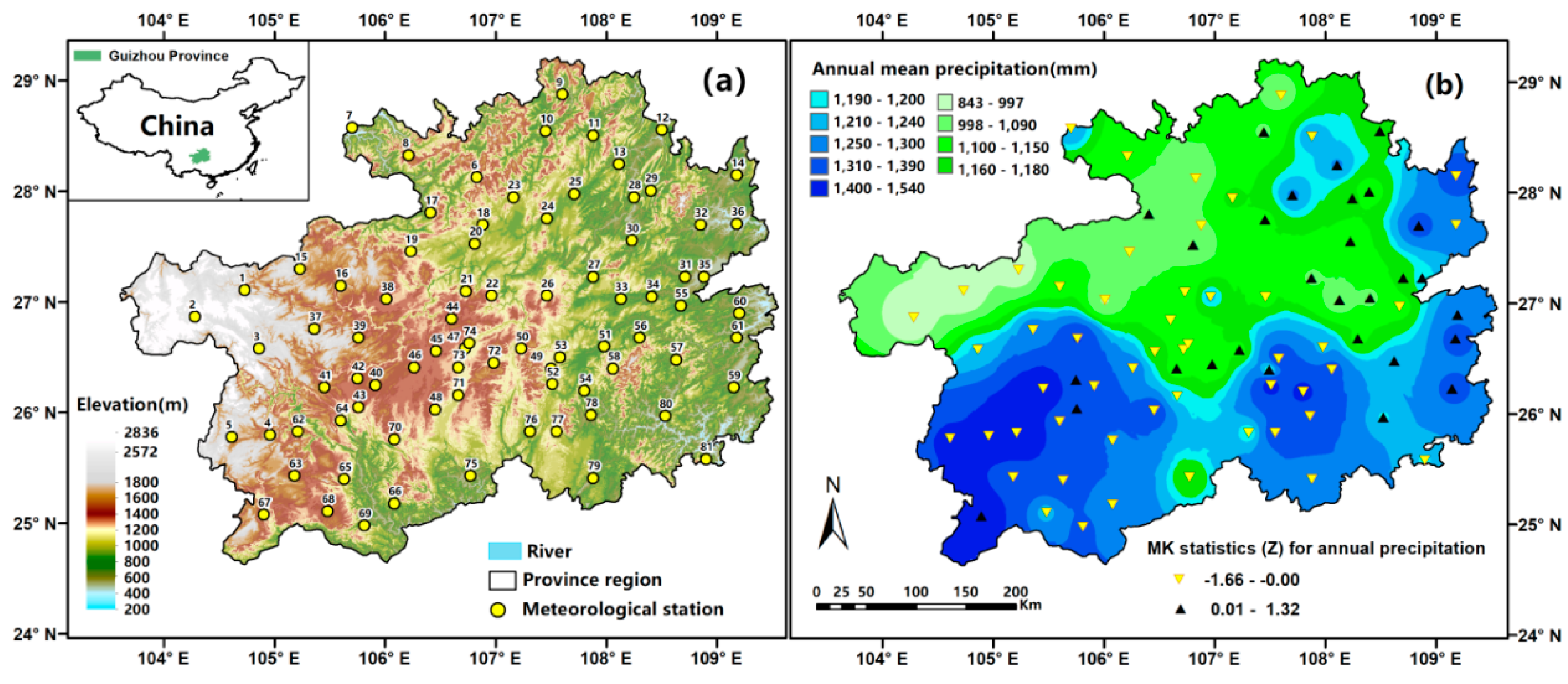
The study region is located in Guizhou Province, Southwest China (Figure 1). It extends from 103°36′ E to 109°35′ E longitude and 24°37′ N to 29°13′ N latitude, with a total area of 176,167 km2. Across the entire region, the mountainous plateau accounts for nearly 87% of the regional area. The topography within the region descends from west to east, varying greatly from 2900 to 148 m in elevation. Its climate, which is characterized by the subtropical wet monsoon, displays an extremely uneven distribution in space and time. Mean annual precipitation ranges 1100–1300 mm and is higher in the south and lower in the north (Figure 1b). About 80% of the annual precipitation is concentrated in the months of April–October. Guizhou Province is located in the center of the karst regions in Southwest China, covered almost entirely by karst landscape. Due to its shallow soils (less than 50 cm in regional mean) [30] and rich rock fractures in the karst areas, flush flows from the high mountains moving to the low depressions often cause floods during the rainfall seasons [31]. Meanwhile, the shallow soils have less capacity in terms of remaining soil moisture storage for agricultural utilization. Therefore, there are frequent occurrences of droughts and floods in the study region. Recently, extreme droughts hit Guizhou Province in 2009, 2011, and 2013, causing an economic loss of 2.3, 5.5, and 9.64 billion Chinese Yuan, respectively [25].
The monthly precipitation records from 1961 to 2004 used for this study are provided by the China Meteorological Administration. The data consist of 81 meteorological stations in Guizhou Province (Figure 1). The missing precipitation data, less than 1% of the total data, are interpolated by averaging records at nearby stations.
A total of four prominent large-scale climatic anomalies were selected to analyze the key drivers of drought events over Guizhou Province: PDO (the Pacific Decadal Oscillation), ENSO (the El Niño-Southern Oscillation), NAO (the North Atlantic Oscillation), and IOD (the Indian Ocean Dipole) [32,33]. The PDO is referred to as a long-lived El-Niño like pattern of the Pacific climate variability and as the leading principal component of monthly SST anomalies in the North Pacific Ocean. The ENSO indicated by the NINO34 index is derived from a SST anomaly in the Niño 3.4 region (5° N–5° S, 170–120° W). The NAO is referred to as a meridional dipole in the atmospheric pressure with centers of action near the Azores and Iceland. The IOD is defined as an anomalous SST gradient between the western equatorial Indian Ocean (10° S–0° N, 50–70° E) and the Southeastern equatorial Indian Ocean (10° S–0° N, 90–110° E). Monthly PDO, NINO34, and NAO data were extracted from the National Oceanic and Atmospheric Administration (https://www.esrl.noaa.gov/psd/ for the period 1961–2004), and monthly values of the IOD index were downloaded from the website (http://www.jamstec.go.jp/frsgc/research/d1/iod/iod/dipole_mode_index.html).
3. Methods
3.1. SPI and Drought Characteristics
Among the drought indices, the Standardized Precipitation Index (SPI) was recommended to characterize meteorological droughts by the World Meteorological Organization [34]. The SPI is space-independent and has demonstrated good performance when representing precipitation anomalies [35,36]. Thus, the index offers the capability to assess drought conditions over a wide range of time scales, while comparison between dry and wet periods at different locations is permitted [13].
In order to derive the SPI series from the long-term precipitation record, precipitation totals were first calculated for a given window of specific dates over a series of years. A probability distribution function was then used to fit the precipitation totals. The fitted distribution function was transformed to the standard normal distribution with a mean of zero and a standard deviation of one [35,37]. Among the probability distribution functions, the most commonly used function is the gamma distribution. The cumulative distribution function of the gamma is given as:
here and are the shape and scale parameters, respectively, estimated by the maximum likelihood method, is the precipitation total, and is the gamma function. Since the gamma function is undefined for , when a precipitation may contain zeros, the cumulative probability becomes
where q is the probability of a zero. If is the numbers of zeros and is the length of the sequence, can be estimated by . After the cumulative probability, , is transformed to the standard normal random variable with mean zero, the value of the SPI can be obtained.
In this study, the precipitation series at a time scale of three months (SPI) was selected as it is capable of representing the seasonal droughts in the study region. A drought event is defined when the SPI value is less than or equal to −1 in a certain period. It can be further classified into different drought severities according to the thresholds of the cumulative probability of SPI (Table 1) [35]. For each of the different drought severities, the drought characteristics of duration (), magnitude (), and peak intensity () shown in Figure 2 can be derived based on the run theory proposed by Yevjevich [38]. The additional characteristic of frequency () is the total number of drought events for different classifications.
3.2. Cluster Analysis for Identifying Similarity of SPI Series Between Sites
Due to the asynchronous variations of the SPI series and the derived drought characteristics between sites, the means of at-site series in any (sub)-regions may underestimate the drought magnitude and extremes [14]. To overcome the shortage, the at-site series in an entire region can be classified into various homogeneous sub-regions or groups. The at-site SPI series in any sub-region vary synchronously to ensure a similarity of drought characteristics between sites and a dissimilarity of drought characteristics between sub-regions.
As one of the most used algorithms in the partitioning cluster method, the K-means clustering algorithm is able to search the synchronous variability of at-site SPI series and classify the homogeneous sub-regions over the study region. The searching is based on the two following criterions using a numerical optimization routine: (1) Minimize the variability of the series at sites within each of the clusters and (2) maximize the variability between clusters. The optimization is to minimize the sum of squares of distances (that is, to maximize the similarity) between the series at individual sites in a cluster and the series at the centroid of the cluster. Here, the centroid is the mean value of the series at sites within a cluster, which is contained in terms of the optimization target of the most significant variance (ANOVA) of the selected series between sites [18].
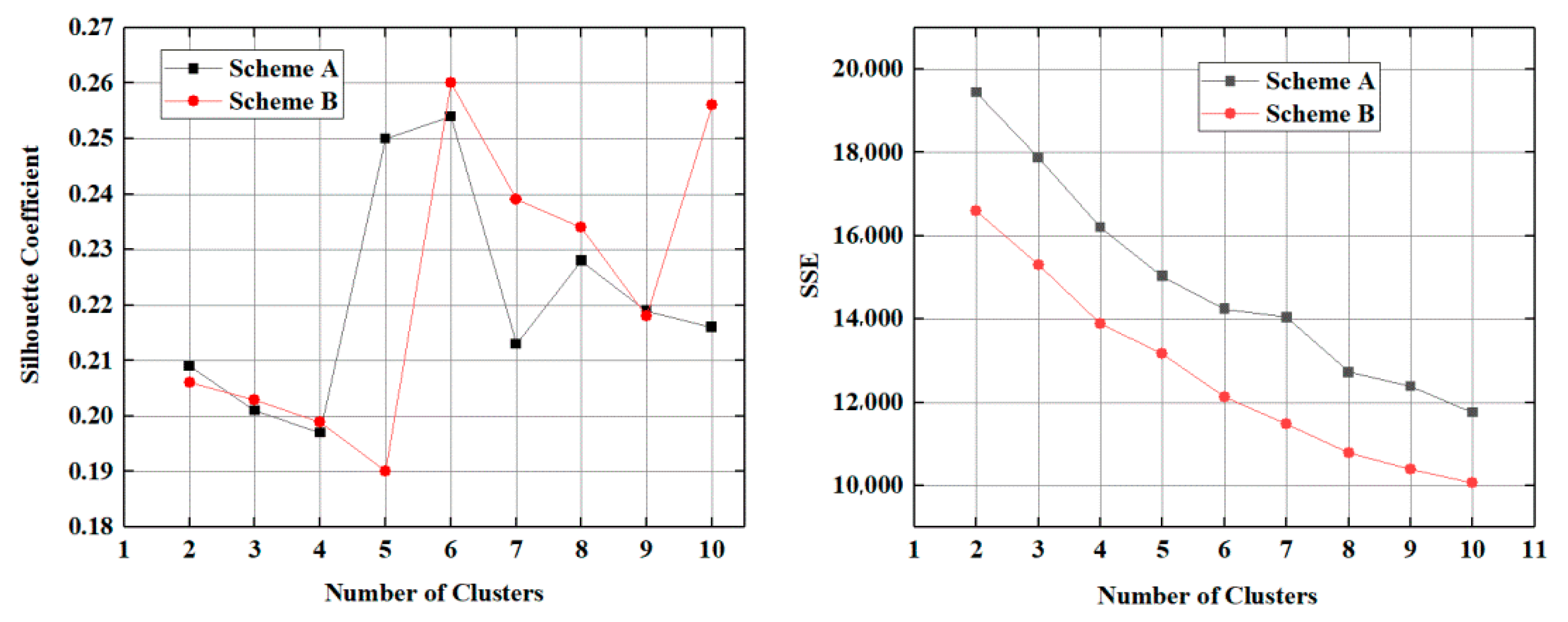
However, the method requires a given number of groups or clusters when the optimization routine is executed. In this study, to search for the best cluster schedule that meets the objective, the silhouette index and sum of squared error (SSE) are used as the two most common measures for time series clusters [17]. The silhouette index [39] is a cluster validation measure. Each cluster is represented by a so-called silhouette (S), which is based on the comparison of its tightness and separation. For the time series at site is computed by:
where is the average dissimilarity of the time series at site to the other members in the same cluster, and is the minimum of average dissimilarity of the time series at site to the members in the other cluster. The varies between −1 and 1, and large values indicate tight and well-separated clusters. When is equal to 1, it means the time series at site is well clustered, while it is equal to 0 it indicates that the time series at site should be assigned to another cluster. The average of for all clusters provides an overall evaluation of clustering validity and can be used to select an appropriate number of clusters [39].
Alternatively, the number of clusters K can be determined when SSE reaches relative stability and becomes acceptable. The SSE is a function that describes the coherence of a given cluster with “better” clusters expected to give lower SSE values. For each time series, the error is the distance to the nearest cluster [17]. In this study, the number “K” is optimized according to the maximum of the average silhouette coefficient and acceptable SSE among comparing the cluster results in a given range of the cluster numbers K, e.g., K = 2–10.
As shown in Figure 2, the entire SPI series at any specific site is composed by non-drought (e.g., SPI > −1) and drought (e.g., SPI ≤ −1) components. The complete SPI series at sites can be directly used to identify the homogeneous sites in a sub-region (Scheme A). In order to reduce the effect of the non-drought SPI component on the similarity identification of the series between individual sites, we pick up drought events (SPI ≤ −1) in the complete SPI series to form a new series. Since occurrences of the drought events could be quite different between the sites, the new series may be too short to meet the standard of drought identification and detection. To obtain a long-term series that covers most of the drought concurrence at all sites, we drew the SPI series at 81 sites to obtain the envelope lines of drought events (SPI ≤ −1). The envelope lines were used to determine the beginning and end times of the drought events for all the sites. A new set of the series at the 81 sites was then used for classifying homogeneous sub-regions (Scheme B). Therefore, there are two schemes (Scheme A and Scheme B) used for classifying the homogeneous sub-regions by the K-means cluster analysis in this study.
3.3. Detection of Spatial and Temporal Evolutions of the Sub-Regional Droughts
3.3.1. Trend Test for the Sub-Regional SPI Series
Long-term trends of sub-regional drought variations and characteristics were analyzed using means of at-site SPI series in each of the homogeneous sub-regions. Since the serial correlation may distort the power of the Mann–Kendall (MK) test, the pre-whitened SPI series that remove lag-1 autocorrelation were used for detecting trends. Here, the trend-free pre-whitening procedure includes three steps. First, an identified trend is removed from the time series that obtains a detrended series, and then, the lag 1 autoregressive process is removed from the detrended series that obtains an independent residual series. Finally, the MK test is applied to the new independent series after removal of the autoregressive component.
The MK test statistic Z is used to identify the degree to which a trend is consistently positive or negative. The significance level was chosen as = 0.05 (1.96 ≤< 2.58) to determine if a trend was statistically significant. Positive values of the statistic indicate upward trends, whereas negative values of the statistic indicate downward trends. The details of the trend-free pre-whitening (TFPW) procedures and the Mann–Kendall test refer to [40,41].
3.3.2. Periodicity Detection for the Sub-Regional SPI Series
After detecting the trend of drought characteristics in any sub-region, the dominant oscillation for the sub-regional SPI time series in monthly scale was analyzed using the continuous wavelet transform (CWT). The CWT can expand a time series into time and frequency space to find localized intermittent periodicities [42]. For a time series {}, the CWT is given by:
where represents the wavelet coefficients,denotes the scale of wavelet, is the time index, denotes the sampling interval, is the mother wavelet, and represents the complex conjugate of the mother wavelet. In this study, the Morlet wavelet was adopted as the mother wavelet function because it can describe the shape of climate index time series. The wavelet power spectrum is the squared modulus of the CWT, used to analyze the dominant periodicities for the SPI oscillation in each of the sub-regions. To examine the statistical significance for the wavelet power spectrum, a background power spectrum was provided by a red noise (a kind of signal noise, increasing power with decreasing frequency) model, and 95% confidence intervals were taken into consideration following Torrence and Campo [43] calculations. As the CWT method assumes the data is cyclic, errors will occur at the beginning and end of the wavelet power spectrum when dealing with finite-length SPI series. Thus, the CWT function creates a cone of influence (COI) that delimitates a region of the wavelet power spectrum. Edge effects become important and the results should be ignored beyond the region of the COI [43].
3.4. Teleconnection of Drought Evolutions with Large-Scale Climate Anomalies
As the wavelet coherence (WCO) can reveal the covariance between two time series, it has been widely used to analyze the drought periodicity and relationships between drought index and possible teleconnections [15,44,45]. In this study, we applied WCO to examine the relationship between SPI and large-scale climate anomaly indices, such as PDO, ENSO, NAO, and IOD. For two time series {} and {}, the cross-wavelet spectrum is given by:
where and are the wavelet power spectrum of {} and {}, respectively. is the complex conjugate of The WCO is defined as the square of the cross-spectrum normalized by the individual power spectrum.
As both time series of the SPI and climate anomaly index generally have obvious red-noise characteristics, the two series can be modeled by a first-order autoregressive (AR1) process. Thus, a large ensemble of surrogate data set pairs with the same AR1 coefficients used as the input dataset will be generated by using Monte Carlo methods. For each pair, the wavelet coherence will be calculated and then used to estimate the significance level. Therefore, the statistical significance ( < 0.05) of the WCO can be determined using Monte Carlo methods with a red-noise spectrum. It usually results in significant periodicities of coherence delineated by significance contours in a figure [44]. In addition, regions beyond the COI should be explained with caution, as well as in the CWT.
4. Results
4.1. Identified Homogeneous Sub-Regions of Drought
On the basis of the monthly precipitation from 1961 to 2004 (44 years) at the 81 meteorological sites (Figure 1), two sets of monthly SPI series (moving average for the time scale of 3 months) at the 81 individual sites was obtained (Scheme A and B). The SPI series at each site for Scheme A has a total number of 528. In contrast, the SPI series at each site for Scheme B selected from the envelope of the drought events has a total number of 422.
Given a range of the number of clusters K (2–10), the K-means cluster method applied for the two schemes gives the overall average silhouette coefficient (S) and the SSE as shown in Figure 3. When the number of clusters is equal to six, the silhouette coefficient (S) reaches the largest value for both schemes and the SSE presents a distinct knee or a change point (reaching a relatively stable status) for Scheme A. Thus, the optimal number of clusters is equal to six for the two schemes. It means that the study region can be classified into six homogeneous sub-regions with the synchronous variation of drought events.
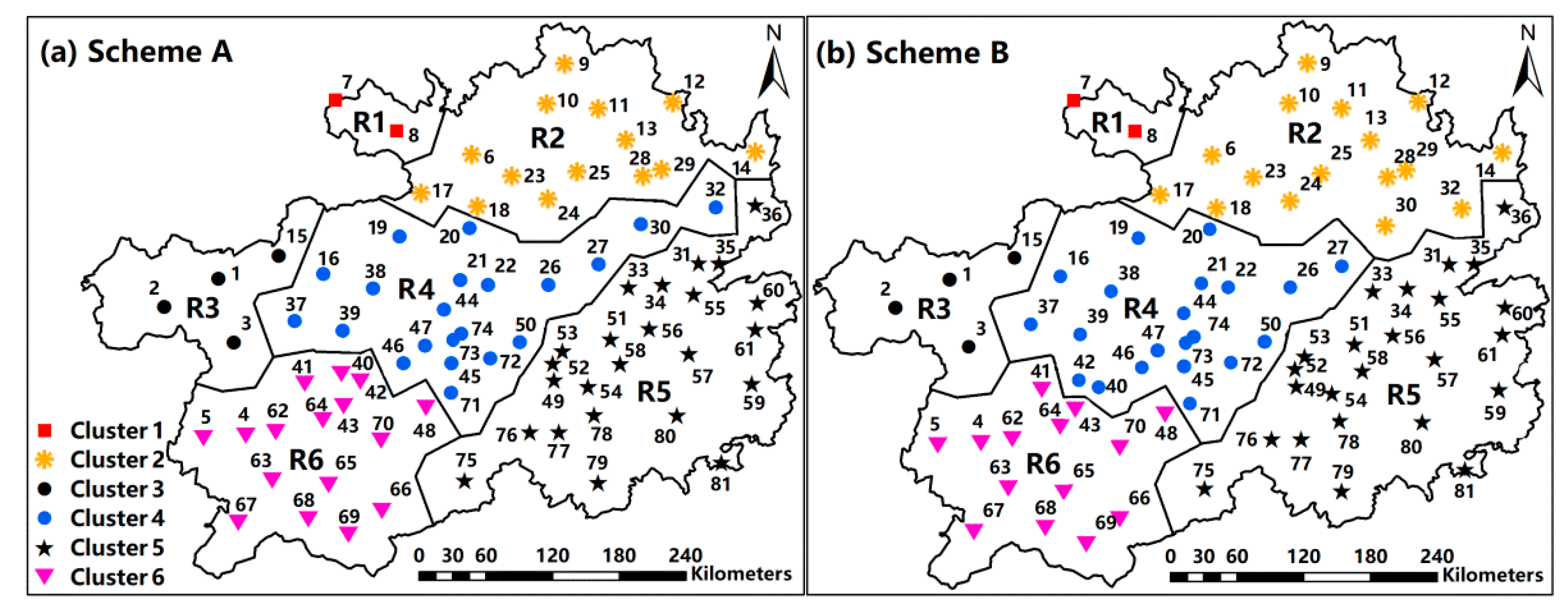
Given the number of clusters “K = 6”, the cluster sites in each sub-region are shown in Figure 4 (a) and (b) for Scheme A and B, respectively. For the two schemes, the clustered sites are the same in sub-regions of R1, R3, and R5, and different in sub-regions of R2, R4, and R6. For example, the sites of 30 and 32 in the northeast are clustered into sub-region R2 for Scheme B and sub-region R4 for Scheme A. The sites of 40 and 42 in the southwest belong to sub-region R4 for Scheme B and sub-region R6 for Scheme A.
Figure 3 shows that the silhouette coefficient was higher in Scheme B than in Scheme A and the SSE was much lower in Scheme B than in Scheme A when the number of clusters was equal to six. In order to compare the cluster results of the two schemes in the same series, drought events in Scheme A were chosen to be same as those in Scheme B for each site. The average silhouette coefficient of Scheme B (SB = 0.190) was also larger than that of Scheme A (SA = 0.185) and the SSE of Scheme B (SSEB = 7029) was slightly larger than that of Scheme A (SSEA = 7006) when the number of clusters was equal to six. It indicates that the cluster results of Scheme B were generally better than those of Scheme A, and thus were used in the subsequent analysis.
According to Scheme B, the geographical locations of the six sub-regions are presented in Figure 4b, displaying large differences in the mean annual precipitation among sub-regions in Figure 1. Four sub-regions are located in high-rainfall centers: R6 in the southwest, R5 in the southeast, R2 in the northeast, and R1 in the north, where mean annual precipitation changes from the highest to the lowest. The left two of R3 and R4 in the northwest are relatively drier (Figure 1 vs. Figure 4b).
4.2. Spatial Characteristics of Sub-Regional Droughts
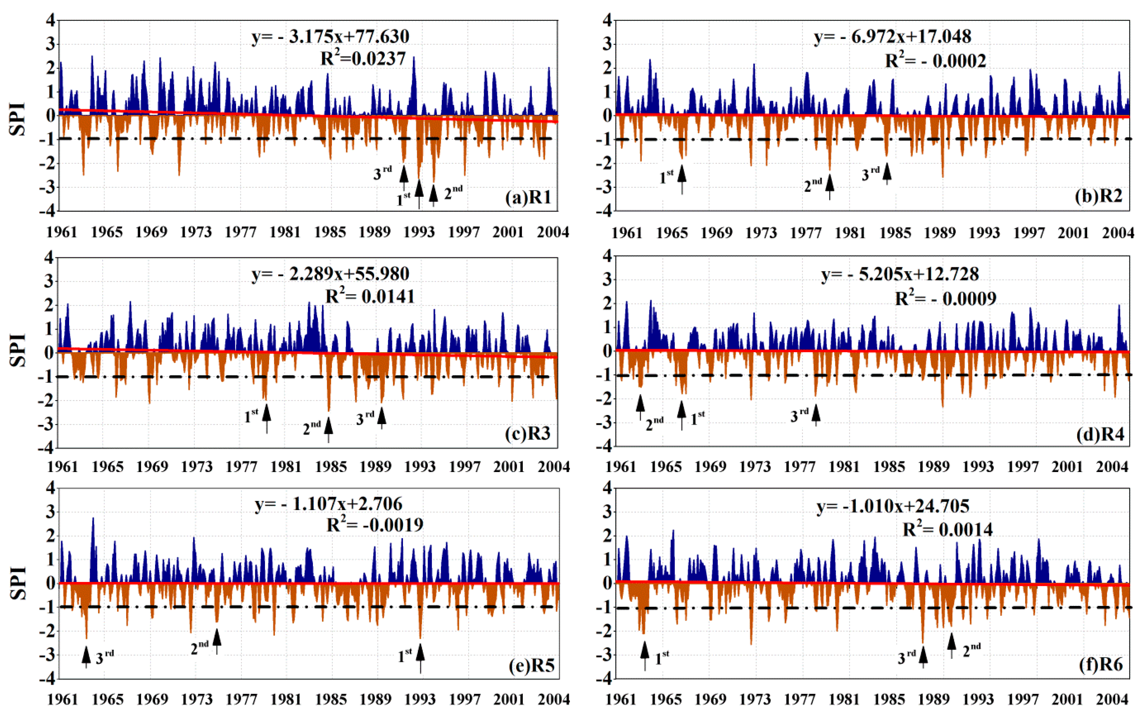
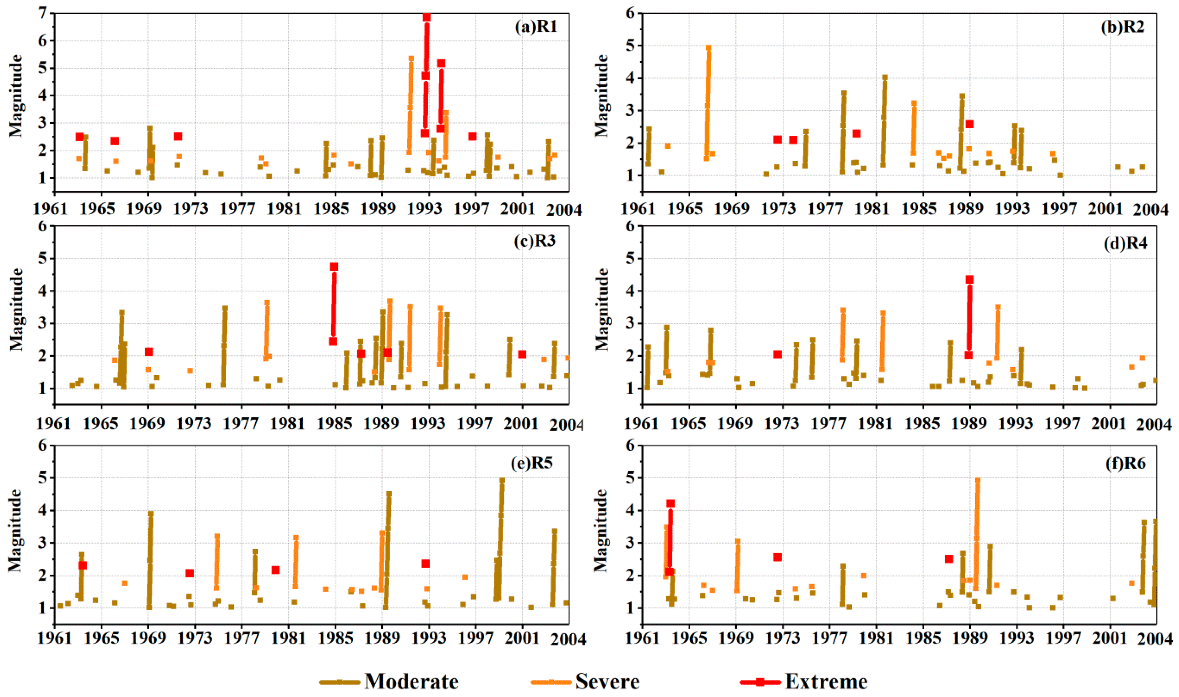
The area-weighted average monthly SPI at sites in any of the sub-regions is used to represent the sub-regional SPI series (Figure 5). Then, drought characteristics (duration , magnitude and peak intensity ) in the sub-regions are derived (Table 2). Furthermore, the moderate, severe and extreme drought events are chosen from the sub-regional SPI series. Temporal evolutions of drought magnitude of the selected events in the six sub-regions are shown in Figure 6.
Drought characteristics and their temporal evolutions were quite different among the six sub-regions. According to drought characteristics in the six sub-regions (Table 2), the drier sub-regions of R3 and R4 had the highest frequency of drought (39) while the wetter sub-region of R6 had the smallest frequency of drought (31). In terms of mean and maximum , , and , the most severe drought area was located in the north (R1), where mean and maximum , and were largest among the six sub-regions (Table 2 and Figure 6). There were six extreme drought events (SPI ≤ −2.0) during the study period, with the least severe drought area located in R2 and R4 in the northeast and center where mean and maximum and were smaller (Table 2 and Figure 6). There were four and two extreme droughts (SPI ≤ −2.0), respectively, during the study period (Table 2 and Figure 6).
The temporal evolution of the drought magnitude for the moderate, severe, and extreme drought events is shown in Figure 6. The moderate droughts occurred most frequently in the study period for each sub-region. The severe and extreme droughts were concentrated in some specific periods, the occurrence of which was different for the six sub-regions. More consecutive occurrences of the severe and extreme drought events could be identified in the period from the late 1980s to the early 1990s in R1 and R3. They were frequent and sporadic occurrences before the early 1990s but few occurrences after the late 1990s in R2 and R4. Comparatively, the severe and extreme drought events in the wet south sub-regions of R5 and R6 occurred occasionally.
If we further select the three most severe drought events, ranked in terms of drought magnitude and duration in each sub-region (e.g., magnitude greater than 4.5 and duration longer than 3 months), the drought occurrences and characteristics are listed in Table 3. The three most severe drought events detected occurred in the early 1960s to the early 1990s in the study region (Table 3 and Figure 6). The characteristics of the most severe drought events were markedly different among sub-regions. Even for a drought event that occurred in the same period/year, the severity could be different in different sub-regions. For example, both sub-regions of R5 and R6 in the south experienced a severe drought in 1963, but the drought duration and magnitude were greater in R6 than in R5 (Table 3 and Figure 6). Another example is the severe drought event in 1992 that occurred in the north and south sub-regions of R1 and R5, respectively. This drought in R1 lasted 6 months (October 1992–January 1993) and had a magnitude of 11.22 and peak of 2.62, whereas this drought in R5 was shorter (4 months from September 1992 to December 1992) and had a smaller and (6.19 and 2.35, respectively). The adjacent sub-regions, such as sub-regions of R1 and R2 in the north, could represent very different drought evolutions (the three most severe drought events occurred in the early 1990s for R1, and in 1966, 1979, and 1984 for R2 in Table 3). The drought severity was much greater in R1 than in R2, as indicated by much smaller values of (3–4 months), (4.54–4.93), and (1.70–2.28) in R2 than those in R1 (Table 3).
As shown in Table 3, the three most severe drought events in the six sub-regions were detected to occur in any season. They occurred more frequently in spring and winter (December–February), (March–May) and autumn (September–November), and less in summer (June–August).
4.3. Temporal Evolution of the Sub-Regional Drought Characteristics
In addition to the spatial difference of drought characteristics among the sub-regions, the temporal evolution of the sub-regional drought characteristics was also different. Here, the temporal evolution was evidenced by the trend and periodicity of the SPI series and the derived , and in the study period. Table 4 listed the detected trends of drought characteristics. The negative values of the monthly SPI series in all sub-regions in Table 4 indicated decreases in the SPI, which were most significant in the western parts of the region (R1, R3, and R6) at the 5% significance level. The decreasing trends of the SPI indicate that the climate tended to be drier. Nevertheless, in terms of trends of the drought characteristics of , and , the evolution of drought severity could be either intensified or weakened as indicated by the positive/negative values of trends of , and/or in Table 4. Thus, trends of , , and could be inconsistent with that of the SPI. In the three sub-regions where decreasing trends of the SPI were significant, the drought severity was intensified in the northwest of R1 and R3, while it was weakened in the southeast of R6.
Cycles or periodicities of the temporal variability in the sub-regions were shown in Figure 7. According to the statistical identification at the 5% significance level, periodicities of the drought variations were significant in a range of 4–48 months for R1, R4, and R6, and 4–36 months for R2, R3, and R5 (Table 5). The high-power variations with a shorter periodicity between 4–12 months were mostly discretely distributed in the period of 1961–2004 for the six sub-regions, but the periodicity that was concentrated in specific periods could be distinguished for some sub-regions. The shorter dominant periodicity was tested to occur in the late 1980s–1990s for the sub-regions of R2, R4, and R6 (Figure 7 and Table 5). Another longer periodicity over 12 months appeared in the periods: Before the early 1970s for the sub-regions in the western parts (R1, R3, R4, and R6), and around the late 1970s to the early 1980s and the late 1990s to early 2000s for the sub-regions of R2 and R5, respectively, in the eastern parts of the study region (Table 5 and Figure 7).
Additionally, except for R1 and R3, the other four sub-regions had two dominant periodicities. The longer periodicities (≥12 months) were mostly concentrated in the early study period, while the shorter significant periodicities (<12 months) were concentrated in the later study period. The shorter the periodicity was, the higher the frequency variability of the cycle was. Thus, as the climate tended to be drier, drought frequency increased in the study region.
4.4. Coherence between Sub-Regional Droughts and Large-Scale Anomaly Climate Indices
The wavelet coherence (WCO) identifies both frequency bands and time intervals of the co-variations between SPI and large-scale climate indices (i.e., PDO, NINO34, NAO, and IOD) over the six sub-regions (Figure 8). The WCO varies as a value from 0 and 1, which measures the cross-correlation between SPI and climate indices as a function of frequency. The colored shading represents the magnitude of the coherence, as shown in the color bar, indicating the timescale variability in the correlation between the two time series. The black contours represent the significant sections that have a 5% significance level. If the SPI and climate indices series are physically related, following the theory of Grinsted [42], we would expect that there is a consistent or slowly varying phase lag, and also expect that the phase arrows should point only in one direction in Figure 8. Thus, the relative phase relationships between the SPI and climate index series are shown as arrows (with in-phase pointing right, indicating positive correlation, and out of phase pointing left indicating negative correlation). In Figure 8, the straight upward (downward) arrow indicates that the sub-regional SPI series lags (leads) the climate index series in phase by 90° [42].
As shown in Figure 8, for a shorter periodicity of less than one year, a significant coherence between SPI and the climate indices was observed intermittently from year to year. However, frequencies of their occurrences in the study period were different in the six sub-regions. As shown in Figure 8, the shorter variations of SPI were less frequently influenced by PDO in R1 and R6, and by NINO34 in R3. Meanwhile, in a specific sub-region, the shorter variations of SPI were coherent with different climate indices in different study periods. For example, for the short periodicity of 4–8 months in R1, SPI was significantly coherent, with PDO around 1968–1983 and with NINO34 around 1983–1998 (Figure 8a,b). Specifically, the shorter dominant periodicity of droughts (Table 5) appearing around the 1990s was always of significant coherence with IOD, which can be observed in sub-regions of R2, R4, and R6. Meanwhile, towards the wetter sub-regions, such as R4 and R6, drought variations tend to be teleconnection with more climate indices.
For the longer periodicity of over a year, the NAO had a leading relationship with drought variation in a period of 30–60 months, appearing before the early 1970s in the western parts of the study region (R1, R3, R4, and R6) (see the yellow part in Figure 8 and Table 5). After the late 1970s, the dominant longer periodicities appeared, such as 16–32 months around 1979–1984 in R2, 12–20 months around 1991–1994, and 24–36 months around 1996–2002 in R5 (Table 5), showing significant in-phase coherence between SPI and NINO34. For the two dominant periodicities in R5, significant in-phase coherence between SPI and NINO34 and anti-phase coherence between SPI and IOD can be observed. Overall, in the entire period of 1961–2004, the dominant influences of the large-scale climate indices on the drought evolutions have been shifted from NAO before the early 1970s to IOD after the late 1970s in the study region.
The three most severe drought events in the six sub-regions (Table 3) were significantly associated with one or more climate indices (Table 6). Comparatively, NINO34 strongly influenced drought variations for most events, representing the significant in-phase coherence. The most severe drought events before the early 1970s always correlated with NAO, with a periodicity from half a year to five years (e.g., first rank in R2, R4, and R6, second rank in R4, and third rank in R5 in the three most severe drought events), but NAO seldom influences the drought events after the 1990s. Some of the events are additionally correlated with PDO, NINO34, or IOD. The drought variations are strongly influenced by IOD for the sub-regions towards the wet south (R4, R5, and R6).
5. Discussions and Conclusions
This study obtained a full description of spatial and temporal evolutions of droughts in Guizhou Province, Southwest China based on the detailed observed data for identifying homogeneous sub-regions and detecting the temporal trends, periodicities, and teleconnection of drought events and their characteristics (i.e., duration, magnitude, and peak) during 1961–2004. The cluster analysis showed that the study region could be classified into six homogeneous sub-regions where the drought characteristics and their temporal evolutions were different. The sub-regional SPI series could be effectively used to distinguish spatial drought characteristics and their temporal evolutions. Droughts were detected to be most severe in the north of the study region (R1) and least severe in the northeast and central sub-regions of R2 and R4 (Table 2), indicated by the largest and smallest mean , and , respectively. The decreasing trend of the SPI series was detected in the region, which was consistent with other studies [25,26,27,28,29]. Spatially, the trend was significant in the western parts of the region (R1, R3, and R6) at the 5% significance level. However, it was found that the decreasing trend of SPI did not mean an intensified drought severity in terms of characteristics of duration , magnitude and peak . The analysis indicated that the decreasing trend of SPI series reflected an overall drier tendency, whereas the trend of drought severity mostly depended on the time of occurrence of extreme drought events. For example, among the three SPI series tested to have significant decreasing trends, the increasing trend of drought severity (,, or ) in R1 and R3 was contributed to by extreme droughts that occurred in the later period (e.g., the 1980s), while the decreasing trend in terms of drought severity in R6 was caused by extreme droughts that occurred in the earlier 1960s (Figure 6).
The significant periodicity was less than 36–48 months in the six sub-regions, including two dominant periodicities of shorter than and longer than one year. These periodicities were concentrated before the early 1970s, the late 1970s to the early 1980s, and 1990s. The shorter periodicity of less than one year appeared in the later period (e.g., in the 1990s for the sub-regions of R2, R4, and R6 in Table 5), commonly caused by IOD. In contrast, the longer periodicity of over one year mostly appeared in the early period (e.g., before the early 1980s in R1–R4 and R6 in Table 5), mainly induced by NAO and NINO34. The temporal evolution of the shortened periodicity from the early to the later period was coincident with the drier trend. The three most severe drought events in the six sub-regions were highly related to the two dominant periodicities and the climate anomaly indices. The most severe drought events significantly linked with NINO34, in addition to NAO and IOD.
The climate of Guizhou Province, Southwest China is dominated by the East Asian summer monsoon and South Asian monsoon (Indian summer monsoon) [46]. The former is significantly influenced by the El Niño-Southern Oscillation (ENSO) through an anomalous lower-tropospheric anticyclone (cyclone) located in the Western North Pacific [47,48], exhibiting a remarkable influence on the interannual variability of the climate over East Asia [49,50]. Meanwhile, the circulation anomaly over Southwest China could also be induced by remote forcing from the tropical Pacific and North Atlantic Oceans (NAO) [20]. Additionally, the intensity of the IOD was characterized by an anomalous SST gradient between the western equatorial Indian Ocean and the southeastern equatorial Indian Ocean. The anomalous heating over the North Indian Ocean could decrease the north–south heating gradient, which is favorable for a weak Indian summer monsoon flow and thus leads to weak water vapor transport to Southwest China [51]. The results indicated that dominant influences of the large-scale climate indices on the drought evolutions had been shifted in the study region, i.e., from NAO before the early 1970s to IOD after the late 1970s, and NINO34 exerted a significant influence on the most extreme drought events. It indicates that the circulation anomaly over Southwest China induced by remote forcing from North Atlantic Oceans (NAO) was weakened while that from ENSO (NINO34) was enhanced after the late 1970s. It follows analysis results by Zhang et al. [23] that a nonconventional El Niño is supposed to be a principal factor of the severe drought in autumn 2009 due to decreased autumn precipitation in Southwest China. Our analysis shows that the anomalous SST gradient by IOD appeared over three consecutive years in the 1990s, causing more severe and extreme droughts in the study region, indicated particularly by the significant a shorter periodicity of less than one year in the southwest, central, and northeast sub-regions of R2, R4, and R6. It follows the analysis results by [52] that the rising autumn positive SST of East Asia (SST of Indian Ocean, South China Sea, and Northwestern Pacific) caused significantly decreasing autumn precipitation over the karst area in Southwest China.
The statistical analysis results were highly dependent on representatives of observational data, such as data lengths, spatial density, and critical criterions used for cluster, trend, and periodicity analysis. Additionally, analysis from the global and regional climate models could offer physical dynamics of climate change and improve the reliability of the analysis results.
Author Contributions
Conceptualization and Formal Analysis, L.X. and X.C.; Methodology, L.X. and R.Z.; Resources, X.C. and Z.Z.; Data curation, Z.Z.; Writing—original draft preparation, L.X.; Writing—review and editing, L.X., R.Z. and X.C.; Supervision, X.C.; Project administration, X.C.; Funding acquisition, X.C.
Funding
This research was funded by the UK-China Critical Zone Observatory (CZO) Program grant number (41571130071), the National Natural Science Foundation of China grant number (41701016 and 51309130), and the Education Department of Jiangxi Province grant number (GJJ180923).
Acknowledgments
We would like to thank the reviewers for their constructive comments that led to significant improvements to the paper.
Conflicts of Interest
The authors declare no conflict of interest.
Abbreviations
| SPI | Standardized precipitation index |
| SPEI | Standardized precipitation evapotranspiration index |
| PDSI | Palmer drought severity index |
| SWSI | Surface water supply index |
| RDI | Reconnaissance drought index |
| CI | Comprehensive meteorological drought index |
| SAD | Severity–area–duration |
| EOF | Empirical orthogonal function |
| REOF | rotated empirical orthogonal function |
| PCA | Principal component analysis |
| CA | Cluster Analysis |
| SST | Sea surface temperature |
| PDO | Pacific Decadal Oscillation |
| ENSO | El Niño Southern Oscillation |
| NAO | North Atlantic Oscillation |
| IOD | Indian Ocean Dipole |
| NINO34 | Niño 3.4 (5° N–5° S, 120°–170° W) sea surface temperature index |
| D | Drought duration |
| M | Drought magnitude |
| P | Drought peak |
| F | Drought frequency |
| ANOVA | Analysis of variance |
| SSE | Sum of Squared Error |
| S | Silhouette index |
| MK | Mann–Kendall trend test |
| TFPW | Trend-free pre-whitening |
| CWT | Continuous wavelet transform |
| WCO | wavelet coherence |
| COI | Cone of influence |
| AR1 | first order autoregressive |
References
- Vicente-Serrano, S.M.; Beguería, S.; López-Moreno, J.I. A multi-scalar drought index sensitive to global warming: The Standardized precipitation evapotranspiration index-SPEI. J. Clim. 2010, 23, 1696–1718. [Google Scholar] [CrossRef]
- Palmer, W.C. Meteorological Drought; US Department of Commerce, Weather Bureau: Washington, DC, USA, 1965; Volume 30.
- Shafer, B.A.; Dezman, L.E. Development of a Surface Water Supply Index (SWSI) to Assess the Severity of Drought Conditions in Snowpack Runoff Areas. In Proceedings of the 50th Annual Western Snow Conference, Reno, NV, USA, 19–23 April 1982; pp. 164–175. [Google Scholar]
- Sheffield, J.; Wood, E.F. Characteristics of global and regional drought, 1950–2000: Analysis of soil moisture data from off-line simulation of the terrestrial hydrologic cycle. J. Geophys. Res. 2007, 112. [Google Scholar] [CrossRef]
- Sheffield, J.; Wood, E.F. Global Trends and Variability in Soil Moisture and Drought Characteristics, 1950–2000, from Observation-Driven Simulations of the Terrestrial Hydrologic Cycle. J. Clim. 2008, 21, 432–458. [Google Scholar] [CrossRef]
- Patel, N.R.; Chopa, P.; Dadhwal, V.K. Analyzing spatial patterns of meteorological drought using Standardized Precipitation Index. Meteorol. Appl. 2007, 14, 329–336. [Google Scholar] [CrossRef]
- Vicente-Serrano, S.M. Differences in spatial patterns of drought on different time scales: An analysis of the Iberian Peninsula. Water Resour. Manag. 2006, 20, 37–60. [Google Scholar] [CrossRef]
- Lloyd-Hughes, B. A spatio-temporal structure-based approach to drought characterization. Int. J. Climatol. 2012, 32, 406–418. [Google Scholar] [CrossRef]
- Xu, K.; Yang, D.W.; Yang, H.B.; Li, Z.; Qin, Y.; Shen, Y. Spatio-temporal variation of drought in China during 1961–2012: A climatic perspective. J. Hydrol. 2015, 526, 253–264. [Google Scholar] [CrossRef]
- Haslinger, K.; Bloschl, G. Space-time patterns of meteorological drought events in the European Greater Alpine Region over the past 210 years. Water Resour. Res. 2017, 53, 9807–9823. [Google Scholar] [CrossRef]
- Guo, H.; Bao, A.M.; Ndayisaba, F.; Liu, T.; Jiapaer, G.; El-Tantawi, A.; Maeyer, P.D. Space-time characterization of drought events and their impacts on vegetation in Central Asia. J. Hydrol. 2018, 564, 1165–1178. [Google Scholar] [CrossRef]
- Andreadis, K.M.; Clark, E.A.; Wood, A.W.; Hamlet, A.F.; Lettermaier, D.P. Twentieth-century drought in the conterminous United States. J. Hydrometeorol. 2005, 6, 985–1001. [Google Scholar] [CrossRef]
- Koutroulis, A.G.; Vrohidou, A.E.K.; Tsanis, I.K. Spatiotemporal Characteristics of Meteorological Drought for the Island of Crete. J. Hydrometeorol. 2011, 12, 206–226. [Google Scholar] [CrossRef]
- Zhou, H.; Liu, Y.B. SPI based meteorological drought assessment over a humid basin: Effects of processing schemes. Water 2016, 8, 373. [Google Scholar] [CrossRef]
- Guo, H.; Bao, A.M.; Liu, T.; Jiapaer, G.; Ndayisaba, F.; Jiang, L.L.; Kurban, A.; De Maeyer, P. Spatial and temporal characteristics of droughts in Central Asia during 1966–2015. Sci. Total Environ. 2018, 624, 1523–1538. [Google Scholar] [CrossRef] [PubMed]
- Vicente-Serrano, S.M. Spatial and temporal analysis of droughts in the Iberian Peninsula (1910–2000). Hydrol. Sci. J. 2006, 51, 83–97. [Google Scholar] [CrossRef]
- Aghabozorgi, S.; Shirkhorshidi, A.S.; Wah, T.Y. Time-series clustering—A decade review. Inf. Syst. 2015, 53, 16–38. [Google Scholar] [CrossRef]
- Santos, J.F.; Pulido-Calvo, I.; Portela, M.M. Spatial and temporal variability of droughts in Portugal. Water Resour. Res. 2010, 46, 742–750. [Google Scholar] [CrossRef]
- Wang, C.L.; Zhong, S.B.; Yao, G.N.; Huang, Q.Y. BME spatiotemporal estimation of annual precipitation and detection of drought hazard clusters using space-time scan statistics in Yun-Gui-Guang region, mainland china. J. Appl. Meteorol. Clim. 2017, 56, 2301–2316. [Google Scholar] [CrossRef]
- Feng, L.; Li, T.; Yu, W. Cause of severe droughts in Southwest China during 1951–2010. Clim. Dyn. 2014, 43, 2033–2042. [Google Scholar] [CrossRef]
- Wang, L.; Chen, W.; Zhou, W.; Huang, G. Teleconnected influence of tropical northwest Pacific sea surface temperature on interannual variability of autumn precipitation in southwest China. Clim. Dyn. 2015, 45, 2527–2539. [Google Scholar] [CrossRef]
- Wang, L.; Chen, W.; Zhou, W.; Huang, G. Drought in Southwest China: A review. Atmos. Oceanic Sci. Lett. 2015, 8, 339–344. [Google Scholar]
- Zhang, W.; Jin, F.F.; Zhao, J.X.; Qi, L.; Ren, H.L. The possible influence of a nonconventional El Niño on the severe autumn drought of 2009 in southwest China. J. Clim. 2013, 26, 8392–8405. [Google Scholar] [CrossRef]
- Huang, R.H.; Liu, Y.; Wang, L.; Wang, L. Analyses of the causes of severe drought occurring in southwest China from the fall of 2009 to the spring of 2010. Chin. J. Atmos. Sci. 2012, 36, 443–457. (In Chinese) [Google Scholar]
- Cheng, Q.P.; Gao, L.; Chen, Y.; Liu, M.B.; Deng, H.J.; Chen, X.W. Temporal-Spatial Characteristics of Drought in Guizhou Province, China, Based on Multiple Drought Indices and Historical Disaster Records. Adv. Meteorol. 2018, 2018, 4721269. [Google Scholar] [CrossRef]
- Yang, P.; Xiao, Z.N.; Yang, J.; Liu, H. Characteristics of clustering extreme drought events in China during 1961–2010. Acta Meteorol. Sin. 2013, 27, 186–198. [Google Scholar] [CrossRef]
- Li, X.; He, B.B.; Quan, X.W.; Liao, Z.M.; Bai, X.J. Use of the standardized precipitation evapotranspiration index (SPEI) to characterize the drying trend in southwest China from 1982–2012. Remote Sens. 2015, 7, 10917–10937. [Google Scholar] [CrossRef]
- Feng, Y.; Cui, N.B.; Xu, Y.M.; Zhang, Z.P.; Wang, J.Q. Temporal and spatial distribution characteristics of meteorological drought in Guizhou Province. J. Arid. Land. Resour. Environ. 2015, 29, 82–86. (In Chinese) [Google Scholar]
- Chen, X.K.; Xu, J.X.; Lei, H.J.; Hu, J.P. Spatial and temporal distribution characteristics of drought and its regional response to climate change in Guizhou province. J. Irrig. Drain. 2015, 34, 72–81. (In Chinese) [Google Scholar]
- Zhang, Z.C.; Chen, X.; Cheng, Q.B.; Peng, T.; Zhang, Y.F.; J, Z.H. Hydrogeology of Epikarst in Karst Mountains—A case study of the Chenqi Catchment. Earth Environ. 2011, 39, 19–25. (In Chinese) [Google Scholar]
- Yin, Z.Y.; Cai, Y.L.; Zhao, X.Y.; Chen, X.L. An analysis of the spatial pattern of summer persistent moderate-to-heavy rainfall regime in Guizhou Province of Southwest China and the control factors. Theor. Appl. Climatol. 2009, 97, 205–218. [Google Scholar] [CrossRef]
- Xiao, M.Z.; Zhang, Q.; Singh, V.P. Influences of ENSO, NAO, IOD and PDO on seasonal precipitation regimes in the Yangtze River basin, China. Int. J. Climatol. 2015, 35, 3556–3567. [Google Scholar] [CrossRef]
- Deng, S.L.; Chen, T.; Yang, N.; Qu, L.; Li, M.C.; Chen, D. Spatial and temporal distribution of rainfall and drought characteristics across the pearl river basin. Sci. Total Environ. 2018, 619, 28–41. [Google Scholar] [CrossRef] [PubMed]
- World Meteorological Organization (WMO). Standardized Precipitation Index User Guide; WMO-No. 1090; WMO: Geneva, Switzerland, 2012. [Google Scholar]
- McKee, T.B.; Doesken, N.J.; Kleist, J. The relationship of drought frequency and duration to time scales. In Proceedings of the 8th Conference on Applied Climatology, Anaheim, CA, USA, 17–22 January 1993. [Google Scholar]
- Guttman, N.B. Comparing the Palmer drought index and the standardized precipitation index. JAWRA J. Am. Water Resour. Assoc. 1998, 34, 113–121. [Google Scholar] [CrossRef]
- Lloyd-Hughes, B.; Saunders, M.A. A drought climatology for Europe. Int. J. Climatol. 2002, 22, 1571–1592. [Google Scholar] [CrossRef]
- Yevjevich, V. An Objective Approach to Definitions and Investigations of Continental Hydrologic Droughts; Hydrologic Paper No. 23; Colorado State University: Fort Collins, CO, USA, 1967. [Google Scholar]
- Rousseeuw, P. Silhouettes: A graphical aid to the interpretation and validation of cluster analysis. J. Comput. Appl. Math. 1987, 20, 53–65. [Google Scholar] [CrossRef] [Green Version]
- Yue, S.; Pilon, P.; Phinney, B.; Cavadias, G. The influence of autocorrelation on the ability to detect trend in hydrological series. Hydrol. Process. 2002, 16, 1807–1829. [Google Scholar] [CrossRef]
- Hamed, K.H.; Rao, A.R. A modified Mann-Kendall trend test for autocorrelated data. J. Hydrol. 1998, 204, 182–196. [Google Scholar] [CrossRef]
- Grinsted, A.; Moore, J.C.; Jevrejeva, S. Application of the cross wavelet transform and wavelet coherence to geophysical time series. Nonlinear Proc. Geoph. 2004, 11, 561–566. [Google Scholar] [CrossRef]
- Torrence, C.; Compo, G.P. A practical guide to wavelet analysis. Bull. Am. Meteorol. Soc. 1998, 79, 61–78. [Google Scholar] [CrossRef]
- Timo, Z.E.; Wheater, H.S.; Bonsal, B.; Razavi, S.; Kurkute, S. Historical drought patterns over Canada and their teleconnections with large-scale climate signals. Hydrol. Earth Syst. Sci. 2018, 22, 3105–3124. [Google Scholar] [Green Version]
- Räsänen, T.A.; Lindgren, V.; Guillaume, J.H.A.; Buckley, B.M.; Kummu, M. On the spatial and temporal variability of ENSO precipitation and drought teleconnection in mainland Southeast Asia. Clim. Past 2016, 12, 1889–1905. [Google Scholar] [CrossRef] [Green Version]
- Bao, L.; Wang, N.N.; Ni, Z.Y. Influence of the Tibetan Plateau uplift on climate evolution in southwestern China: From the monsoon perspective. J. Earth Environ. 2018, 9, 444–454. (In Chinese) [Google Scholar]
- Wang, B.; Wu, R.G.; Fu, X.H. Pacific-East Asian teleconnection: How does ENSO affect East Asian climate? J. Clim. 2000, 13, 1517–1536. [Google Scholar] [CrossRef]
- Chen, W.; Feng, J.; Wu, R.G. Roles of ENSO and PDO in the link of the East Asian Winter Monsoon to the following Summer Monsoon. J. Clim. 2013, 26, 622–635. [Google Scholar] [CrossRef]
- Feng, J.; Chen, W.; Tam, C.Y.; Zhou, W. Different impacts of El Niño and El Niño Modoki on China rainfall in the decaying phases. Int. J. Climatol. 2011, 31, 2091–2101. [Google Scholar] [CrossRef]
- Feng, J.; Wang, L.; Chen, W.; Fong, S.K.; Leong, K.C. Different impacts of two types of pacific ocean warming on southeast Asian rainfall during boreal winter. J. Geophys. Res. 2010, 115, D24122. [Google Scholar] [CrossRef]
- Zhang, R.H. Relations of water vapor transport from Indian monsoon with that over East Asia and the summer rainfall in China. Adv. Atmos. Sci. 2001, 18, 1005–1017. [Google Scholar]
- Liu, B.J.; Li, Y.; Chen, J.F.; Chen, X.H. Long-term change in precipitation structure over the karst area of Southwest China. Int. J. Climatol. 2016, 36, 2417–2434. [Google Scholar] [CrossRef]
Figure 1.
Spatial distribution of topography and meteorological stations (a), and mean annual precipitation and changes (increasing or decreasing trend) from 1961 to 2004, and (b) in the study region, yellow triangle denotes insignificantly decreasing trend and black triangle denotes a insignificantly increasing trend at the 0.05 level.

Figure 2.
Sketch of drought characteristics using the SPI.

Figure 3.
Average silhouette coefficient and sum of squared error (SSE) versus number of clusters for Scheme A and B.
Figure 3.
Average silhouette coefficient and sum of squared error (SSE) versus number of clusters for Scheme A and B.

Figure 4.
The clustered sub-regions by Scheme A and B.

Figure 5.
Temporal evolution and trends (red line) of the sub-regional SPI series in six sub-regions (the three most severe drought events ranking first, second, and third are shown with arrows).
Figure 5.
Temporal evolution and trends (red line) of the sub-regional SPI series in six sub-regions (the three most severe drought events ranking first, second, and third are shown with arrows).

Figure 6.
Temporal evolution of drought magnitude for the selected events of moderate, severe, and extreme droughts in six sub-regions.
Figure 6.
Temporal evolution of drought magnitude for the selected events of moderate, severe, and extreme droughts in six sub-regions.

Figure 7.
The power spectrum of continuous wavelet transform (CWT) of the SPI series from 1961 to 2004 for the six sub-regions. The color from blue to yellow indicates the increasing wavelet power. The black contour designates the 5% significance level against red noise and the cone of influence (COI), where the edge effects are not negligible, is shown as a light-shaded area.

Figure 8.
Squared wavelet coherence (WCO) between the large-scale climate indices and sub-regional SPI series. The colors from blue to yellow indicate the increasing coherence. The 5% significance level against red noise is shown as a black contour. The COI where the edge effects are not ignored is shown as a light-shaded area. The relative phase relationship for the two signals is shown as arrows (with in-phase pointing right, out of phase pointing left, climate indices leading SPI by 90° pointing straight up, and SPI leading climate indices by 90° pointing straight down).


Table 1.
Classification of drought and wet conditions based on the Standardized Precipitation Index (SPI).
Table 1.
Classification of drought and wet conditions based on the Standardized Precipitation Index (SPI).
| Categories | SPI | Cumulative Probability |
|---|---|---|
| Wet | 1.0 | (0.841,1.0) |
| Near normal | (−1.0,1.0) | (0.159,0.841) |
| Moderate drought | (−1.5,−1.0) | (0.067,0.159) |
| Severe drought | (−2.0,−1.5) | (0.023,0.067) |
| Extreme drought | −2.0 | (0,0.023) |
Table 2.
Identified drought characteristics for the six sub-regions.
| Sub-Region | R1 | R2 | R3 | R4 | R5 | R6 | |
|---|---|---|---|---|---|---|---|
| Drought frequency () | 37 | 35 | 39 | 39 | 33 | 31 | |
| Drought duration () (months) | Mean | 1.97 | 1.66 | 1.85 | 1.59 | 1.85 | 1.87 |
| Max | 6.00 | 3.00 | 4.00 | 4.00 | 4.00 | 5.00 | |
| Drought magnitude (M) | Mean | 2.94 | 2.33 | 2.52 | 2.16 | 2.52 | 2.71 |
| Max | 11.22 | 4.93 | 6.67 | 5.98 | 6.19 | 7.60 | |
| Drought peak | Mean | 1.57 | 1.49 | 1.43 | 1.38 | 1.47 | 1.55 |
| Max | 2.79 | 2.57 | 2.44 | 2.33 | 2.35 | 2.55 | |
Table 3.
Drought characteristics of the three most severe drought events ranked by magnitude in the six sub-regions from 1961 to 2004.
Table 3.
Drought characteristics of the three most severe drought events ranked by magnitude in the six sub-regions from 1961 to 2004.
| Sub-Region | Rank | Persistent Period (yyyy.mm) | Duration (Months) | Magnitude | Peak Intensity | Peak Time |
|---|---|---|---|---|---|---|
| R1 | 1 | August 1992–January 1993 | 6 | 11.22 | 2.62 | September 1992 |
| 2 | November 1993–February 1994 | 4 | 8.03 | 2.79 | January 1994 | |
| 3 | April 1991–July 1991 | 4 | 6.62 | 1.94 | May 1991 | |
| R2 | 1 | July 1966–September 1966 | 3 | 4.93 | 1.80 | September 1966 |
| 2 | April 1979–June 1979 | 3 | 4.78 | 2.28 | May 1979 | |
| 3 | February 1984–April 1984 | 3 | 4.54 | 1.70 | March 1984 | |
| R3 | 1 | February 1979–May 1979 | 4 | 6.67 | 1.97 | May 1979 |
| 2 | November 1984–January 1985 | 3 | 5.85 | 2.44 | November 1984 | |
| 3 | July 1989–September 1989 | 3 | 5.77 | 2.08 | July 1989 | |
| R4 | 1 | August 1966–November 1966 | 4 | 5.98 | 1.79 | September 1966 |
| 2 | January 1963–April 1963 | 4 | 5.76 | 1.52 | March 1963 | |
| 3 | February 1978–April 1978 | 3 | 4.70 | 1.88 | February 1978 | |
| R5 | 1 | September 1992–December 1992 | 4 | 6.19 | 2.35 | October 1992 |
| 2 | October 1974–January 1975 | 4 | 5.53 | 1.61 | November 1974 | |
| 3 | April 1963–June 1963 | 3 | 4.94 | 2.31 | June 1963 | |
| R6 | 1 | April 1963–August 1963 | 5 | 7.60 | 2.10 | May 1963 |
| 2 | June 1989–October 1989 | 5 | 7.16 | 1.79 | September 1989 | |
| 3 | March 1987–May 1987 | 3 | 5.37 | 2.50 | April 1987 |
Table 4.
Trend of SPI and drought characteristics from 1961 to 2004 in the six sub-regions.
| SPI and Drought Characteristics | R1 | R2 | R3 | R4 | R5 | R6 |
|---|---|---|---|---|---|---|
| Sub-regional SPI | −4.23 * | −1.27 | −3.53 * | −0.90 | −0.41 | −2.13 * |
| Drought duration () | 0.32 | −0.86 | 0.29 | −0.53 | 0.69 | −0.82 |
| Drought magnitude | 0.04 | −1.48 | 0.19 | −1.33 | 0.67 | −1.19 |
| Drought peak | −0.11 | −1.62 | 0.48 | −1.04 | −0.33 | −1.87 |
* indicate the significance at the 0.05 level.
Table 5.
Periodicity of drought variability and its link with climate indices from 1961 to 2004 in the six sub-regions.
Table 5.
Periodicity of drought variability and its link with climate indices from 1961 to 2004 in the six sub-regions.
| Sub-Region | Significant Periods (Month) | Dominant Periods (Month) | Intervals of Variance | Significant Link with Climate Indices |
|---|---|---|---|---|
| R1 | 4–48 | 24–48 | 1964–1972 | NAO |
| R2 | 4–36 | 16–32; 4–12 | 1979–1984; 1991–1997 | NINO34; IOD |
| R3 | 4–36 | 24–36 | 1965–1971 | NAO |
| R4 | 4–48 | 4–12; 32–48 | 1990–1997; 1964–1969 | PDO, NAO, and IOD; NAO |
| R5 | 4–36 | 12–20; 24–36 | 1991–1994; 1996–2002 | NINO34 and IOD; NINO34 and IOD |
| R6 | 4–48 | 32–48; 4–12 | 1964–1968; 1989–1996 | NAO; PDO, NINO34, IOD, and NAO |
Table 6.
The significant link with climate indices for the three most severe drought events in the six sub-regions.
Table 6.
The significant link with climate indices for the three most severe drought events in the six sub-regions.
| Sub-Region | Rank | Persistent Time (yyyy.mm) | PDO Period (Month) | NINO34 Period (Month) | NAO Period (Month) | IOD Period (Month) |
|---|---|---|---|---|---|---|
| R1 | 1 | August 1992–January 1993 | / | 4–10 (←) | / | 24–48 |
| 2 | November 1993–February 1994 | / | 8–24 (→) | / | / | |
| 3 | April 1991–July 1991 | / | 12–30 (→) | / | 4–8, 16–64 | |
| R2 | 1 | July 1966–September 1966 | / | 16–24 (→) | 24–40 | 4–8 |
| 2 | April 1979–June 1979 | 8–16, 32–64 | 12–16 | 6–8 | / | |
| 3 | February 1984–April 1984 | / | 16–32 (→) | / | / | |
| R3 | 1 | February 1979–May 1979 | / | / | 10–16 | / |
| 2 | November 1984–January 1985 | 32–64 | 48–64 (→) | / | / | |
| 3 | July 1989–September 1989 | 4–8 | 48–64 (→) | 4–8 | 6–8 | |
| R4 | 1 | 1966.08–November 1966 | / | / | 16–48 | / |
| 2 | January 1963–April 1963 | 6–16 | / | 6–8, 30–60 | 2–4 | |
| 3 | February 1978–April 1978 | 12–16 | 12–20 (←) | 12–16 | 24–48 | |
| R5 | 1 | September 1992–December 1992 | / | 8–24 (→) | / | 32–64 (→) |
| 2 | October 1974–January 1975 | / | 48–64 (→) | / | 32–64 (→) | |
| 3 | April 1963–June 1963 | / | 16–32 (→) | 32–60 | 20–32 | |
| R6 | 1 | April 1963–August 1963 | 4–6 | 16–24 (→) | 12–16 | / |
| 2 | June 1989–October 1989 | 4–8 | 32–64 (→) | 12–20 | 32–64 (→) | |
| 3 | March 1987–May 1987 | 6–8 | 32–64 (→) | / | 32–64 (→) |
Note: “/” means no significant periods being detected. The relative phase relationship for climate indices and the most severe drought events is shown as arrows (with in-phase pointing right and out of phase pointing left).
© 2019 by the authors. Licensee MDPI, Basel, Switzerland. This article is an open access article distributed under the terms and conditions of the Creative Commons Attribution (CC BY) license (http://creativecommons.org/licenses/by/4.0/).
Share and Cite
MDPI and ACS Style
Xiao, L.; Chen, X.; Zhang, R.; Zhang, Z. Spatiotemporal Evolution of Droughts and Their Teleconnections with Large-Scale Climate Indices over Guizhou Province in Southwest China. Water 2019, 11, 2104. https://doi.org/10.3390/w11102104
AMA Style
Xiao L, Chen X, Zhang R, Zhang Z. Spatiotemporal Evolution of Droughts and Their Teleconnections with Large-Scale Climate Indices over Guizhou Province in Southwest China. Water. 2019; 11(10):2104. https://doi.org/10.3390/w11102104
Chicago/Turabian StyleXiao, Liying, Xi Chen, Runrun Zhang, and Zhicai Zhang. 2019. "Spatiotemporal Evolution of Droughts and Their Teleconnections with Large-Scale Climate Indices over Guizhou Province in Southwest China" Water 11, no. 10: 2104. https://doi.org/10.3390/w11102104
Note that from the first issue of 2016, this journal uses article numbers instead of page numbers. See further details here.