Modified Approach to Reduce GCM Bias in Downscaled Precipitation: A Study in Ganga River Basin

Abstract

Reanalysis data is widely used to develop predictor-predictand models, which are further used to downscale coarse gridded general circulation models (GCM) data at a local scale. However, large variability in the downscaled product using different GCMs is still a big challenge. The first objective of this study was to assess the performance of reanalysis data to downscale precipitation using different GCMs. High bias in downscaled precipitation was observed using different GCMs, so a different downscaling approach is proposed in which historical data of GCM was used to develop a predictor-predictand model. The earlier approach is termed “Re-Obs” and the proposed approach as “GCM-Obs”. Both models were assessed using mathematical derivation and generated synthetic series. The intermodal bias in different GCMs downscaled precipitation using Re-Obs and GCM-Obs model was also checked. Coupled Model Inter-comparison Project-5 (CMIP5) data of ten different GCMs was used to downscale precipitation in different urbanized, rural, and forest regions in the Ganga river basin. Different measures were used to represent the relative performances of one downscaling approach over other approach in terms of closeness of downscaled precipitation with observed precipitation and reduction of bias using different GCMs. The effect of GCM spatial resolution in downscaling was also checked. The model performance, convergence, and skill score were computed to assess the ability of GCM-Obs and Re-Obs models. The proposed GCM-Obs model was found better than Re-Obs model to statistically downscale GCM. It was observed that GCM-Obs model was able to reduce GCM-Observed and GCM-GCM bias in the downscaled precipitation in the Ganga river basin.

1. Introduction

General circulation models (GCM) cannot be directly used for climate studies at regional scale due to coarse spatial resolution. Wood et al. [1] suggested that products of GCMs should not be directly used to assess local or regional scale patterns, as these are less promising, specifically for precipitation. So, downscaling procedures are adopted to bridge the gap of scale mismatch between GCM and local variable. Downscaling of coarse scale GCM to a regional scale is usually done in climate change studies with different downscaling methods. Generally, two downscaling techniques are used, i.e., (i) Statistical downscaling, i.e., based on the statistical relationship between large scale atmospheric variable and local scale observed data, and (ii) Dynamical downscaling, i.e., based on the output of regional climate models (RCM) [2,3,4]. Both downscaling approaches have been thoroughly discussed and documented in different literatures [4,5]. Statistical downscaling is generally used as it requires less computational resources and time than dynamical downscaling. A downscaling approach based on simple manipulation of observed data, i.e., change factor methodology, is also applied in some studies [6] but statistical downscaling methods are most widely used [7]. Pielke et al. [5] discussed different types of statistical and dynamical downscaling based on their purpose and inputs. This study may be classified into type 4 statistical downscaling in which a transfer function between present climate and large-scale atmospheric variables is used to represent the future climate with the help of earth system models representing future climate conditions.

Typically, a statistical relationship between coarse scale atmospheric variables (predictors) and finer scale local observation (predictand) is developed in statistical downscaling techniques. A developed relationship is used to downscale GCM at a local scale. Different methods have been adopted previously to develop the predictor-predictand model based on simple linear regression [8], partial least square regression [9], artificial neural networks [10], relevance vector machines [11], etc. Generally, observations of all atmospheric variables, which are required to develop a predictor-predictand relationship, are not available. So, it is a standard practice to use reanalysis data as predictors in the absence of observed atmospheric variables. Different agencies provide wide ranges of reanalysis data at a global or continental scale [12,13]. The National Center for Environment Prediction (NCEP)/National Center for Atmospheric Research (NCAR) reanalysis data [12] is mostly used in statistical downscaling. Reanalysis data have been widely used to downscale precipitation [8,10,14,15], temperature [16,17], streamflow [18], and other variables. Detailed description of previous studies related to statistical downscaling is covered in different review articles [19,20].

The variability in the values, statistical properties etc., in downscaled variable with different GCMs, is still a big issue for climate researchers. The latest assessment report of the Intergovernmental Panel on Climate Change (IPCC) emphasized the issue of uncertainty in the projection of different GCMs [21]. Uncertainty is also inherited with different GCMs due to differences in parametrization, boundary conditions, and the structure and physics used in driving GCM [19]. Sunyer et al. [22] used statistical downscaling techniques to downscale extreme rainfall events with four GCM driven RCMs and found a significant GCM-GCM bias (difference in downscaled precipitation using different GCMs) in downscaled rainfall. Hughes et al. [23] also showed high variability in downscaled rainfall using nine different GCMs. Ahmed et al. [24] reported the differences in downscaled precipitation and temperature using different GCMs. Climate change detection studies also show variability in the detection of climate change using different GCMs [8,25,26]. The bias in downscaled variables using different GCMs is reported in the latest review studies [27,28]. Jiang et al. [29] addressed the issue of high variability in downscaled products using different GCMs. Pan et al. [30] ran two regional climate models (RCMs) forced by different boundary conditions, i.e., reanalysis, GCM, and future scenarios of GCM. Large differences in downscaled precipitation were observed using different GCMs.

Bias correction methods are generally adopted to reduce this uncertainty. There have been a wide range of bias correction methods proposed by different researchers. A simple quantile-based CDF matching method has been widely used [1,31], which is based on the assumption that climate does not change over time. To overcome this assumption, Li et al. [32] proposed an equidistant CDF matching method which maps the quantile of GCM variable on corresponding value of the model and the difference between observed and model values is added to get the bias corrected value. Some researchers have also a proposed method to correct low frequency bias in a downscaled variable using nesting techniques [33,34]. However, these techniques are unable to correct bias for defined time scales. Nguyen et al. [35] proposed frequency based bias correction method which is time independent and was found to be better than nesting techniques.

The bias correction methods are found to remove some bias and decrease uncertainty in downscaled data. In this study, a different method of downscaling GCM data is proposed which produces less GCM-GCM bias than using reanalysis data. As a case study, CMIP5 historical data of ten different GCMs was used to downscale precipitation in different regions in the Ganga river basin in India. Previous studies in the Ganga river basin show a temperature rise and increase in frequency of extreme events due to climate change [36,37,38,39,40].

Giorgi et al. [41] used the terms “model performance” and “model convergence” for evaluation of the model. Model performance describes the closeness of simulated data to target data and convergence shows uncertainty in different sets of simulated data. The reliability ensemble averaging (REA) technique was used to evaluate the model performance and convergence. REA considers performance in terms of bias from observed data and convergence as a distance from weighted the average of ensemble members to calculate the reliability factor of a model. The reliability of a model was defined as product of its performance and convergence. Dessai et al. [42] used a performance skill score and convergence skill score to evaluate the models. The inverse of the normalized root mean square deviation between simulated and observed data gives a performance skill score. The convergence skill score is also calculated as the inverse of root mean square deviation but between simulated data by a GCM and ensembles average data. The combined skill score was also calculated, which is a weighted product of the performance and convergence skill score, to define the reliability of a model. Most of the previous studies used deviations or root mean square deviation to evaluate the models. In this study different measures, i.e., skill score, correlation, normalized root mean square deviation (NRMSD), etc., were used to judge the reliability of both models.

This study aimed to find the answers for two questions:

(i)

Should reanalysis data be always used to develop a predictor-predictand relationship and to use the same relationship to downscale GCM? and

(ii)

Can a simple change in the downscaling approach be helpful to reduce GCM-GCM bias?

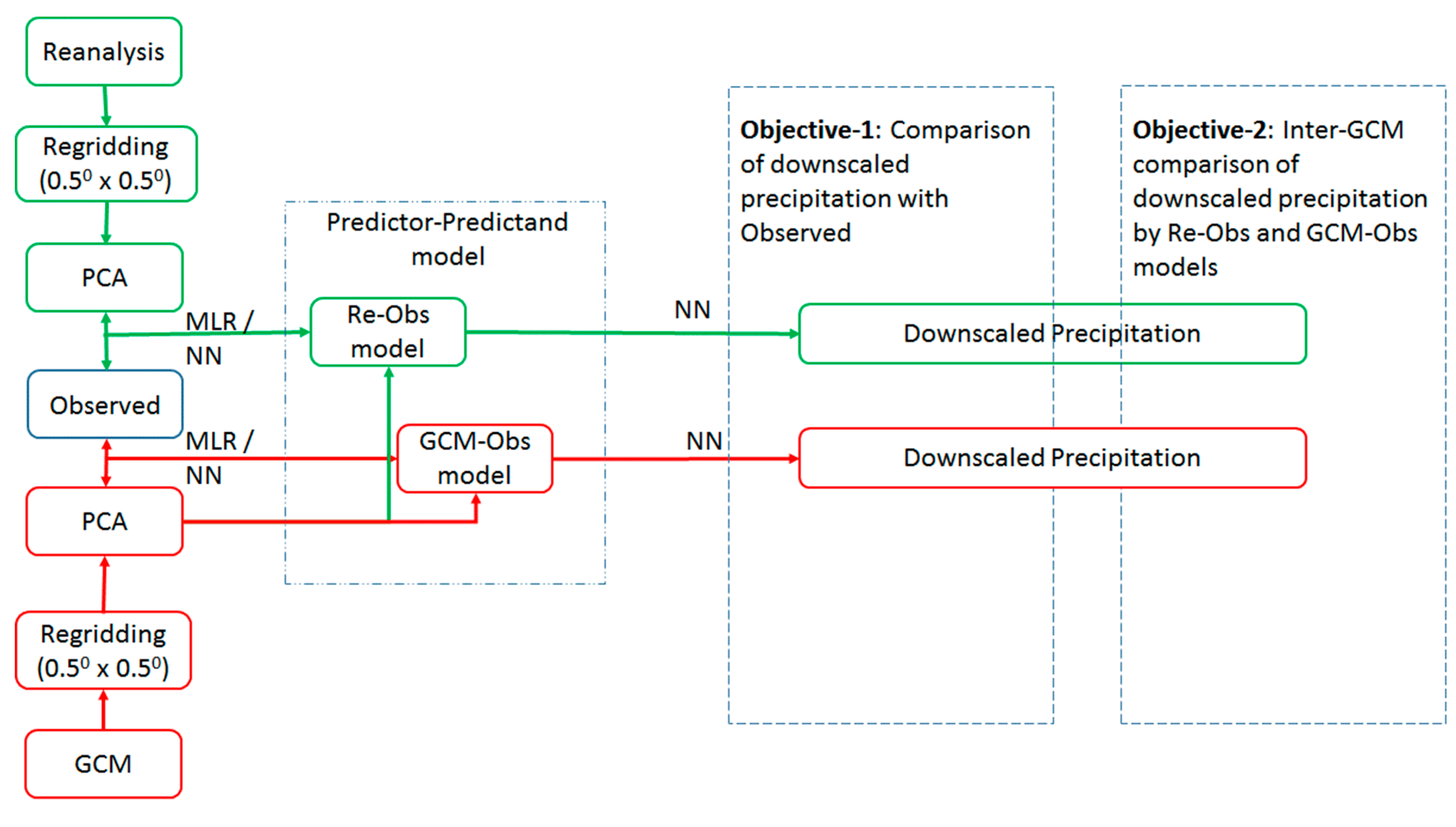
The driving ideologies of this study were that (i) there is always dissimilarity in the predictor sets of reanalysis and GCM data due to difference in their development, so predictor-predictand model based on predictors of reanalysis data might not be good enough to downscale GCMs, and (ii) a better predictor-predictand relationship of reanalysis-observed data does not assure good downscaling will occur with different GCMs. This may be better understood as follows

Say,

$$Observed=f(Obs)$$

(1)

$$\mathrm{Re}analysis=f(Obs1)$$

(2)

$$GCM1=f(G)$$

(3)

$$GCM2=f(G)$$

(4)

Here, ‘Obs’, ‘Obs1′ is the characteristics of observed and reanalysis data time series. As, the reanalysis data is developed using observations, Obs1 is similar to Obs. ‘G’ includes the characteristics of GCM1 and GCM2. GCM1 and GCM2 are GCM products of the same GCM model but with different times.

As a standard statistical approach, Observed, Reanalysis and GCM1 data are available for the same time period, while the GCM2 product have to downscale using the predictor-predictand relationship.

If one wishes to find the unknown value of GCM2 in accordance with the data observed, there may be two approaches:

(i)

‘Re-Obs’—Develop a relationship between Reanalysis and Observed than transfer the relationship to GCM2.

(ii)

‘GCM-Obs’—Develop a relationship between GCM1 and Observed and transfer it to GCM2.

So, it can be observed that GCM-Obs is a better choice as it is using the same group of variables to develop the predictor-predictand relationship which needs to be predicted.

Each GCM simulation is based on assumptions of climate systems, initial conditions, parameterizations, and numerical methods used to solve the non-linear differential equations of the fluid motion of the atmosphere and the ocean [43,44]. The reanalysis data is based on the observation data, so these are closer to the observed data than GCMs. It is obvious that the relationship between reanalysis and observed data may be better than relationship between GCM and observed data. However, this doesn’t guarantee better GCM downscaling. GCM downscaling using the Re-Obs model would be similar to predicting a time series using the relationship of two similar time series which are different from the predicted time series. Racherla et al. [7] also concluded that a better model does not necessarily translate to better climate projections. GCM downscaling using the GCM-Obs model may be the better choice, as the predictor-predictand relationship between GCM and observed data already considers the GCM uncertainty, which may result in better GCM downscaled products that may be close to the observations.

Change Factor Methodologies (CFM) [6] also use a similar approach to downscale GCM. CFM only use GCM data to downscale future GCM by using additive multiplicative measures with observations. CFM is widely used across the world in climate change impact assessment studies and programs [45,46].

An effort had been made in this study to reduce the GCM bias in downscaled products using the predictor-predictand relationship and using historical GCM data itself as the predictor. This technique is referred to as GCM-Obs. Using historical GCM data as the predictor might provide better future projections of respective GCM, as it has already considered the inherent uncertainty of GCM in model development. Change factor methodology also has a similar approach of downscaling which uses the GCM-Obs relationship to downscale future projections of climate.

After the brief introduction and background of the presented study in Section 1, GCM-Obs logic is described using mathematical expressions and synthetic series in Section 2. The Re-Obs and GCM-Obs models are compared using a case study in the Ganga river basin. The study area and data used are described in Section 3, the methodology adopted is given in Section 4, while Section 5 describes the outcome of the study. Discussions are provided in Section 6 followed by limitations in Section 7. The study is concluded in Section 7. A methodology to develop predictor-predictand relationship is described in Appendix A.

Definition 1.

Definition of Bias: The term bias used in this study represents the differences between downscaled precipitation using different GCMs and differences between downscaled and observed precipitation.

2. The GCM-Obs Logic

2.1. Mathematical Explanation

The performance of prediction model can be assessed by checking the deviations of predicted values from observed data. For example, a variable ‘O’ having mean ${\mu }_O$ and standard deviation ${\sigma }_O$ depend on the variable $‘R’$ (${\mu }_R$ and ${\sigma }_R$). It also depends on the variable $‘G’$ (${\mu }_G$ and ${\sigma }_G$). The correlation between $‘O’$ and $‘R’$ is ${\rho }_{OR}$ and between $‘O’$ and $‘G’$ is ${\rho }_{OG}$. Some part of data is considered for training $‘tr’$ and remaining is used for testing $‘ts’$. The simplest relationship between two variables can be defined by a linear regression model.

So,

$O=f\left(R\right)$ and $O=f\left(G\right)$

$${\left(O_{tr}\right)}_i={\alpha }_{R_{tr}}+{\beta }_{R_{tr}}{\left(R_{tr}\right)}_i$$

(5)

$${\widehat{\beta }}_{R_{tr}}={\rho }_{OR}\raisebox{1ex}{${\sigma }_R$}\!\left/ \!\raisebox{-1ex}{${\sigma }_O$}\right.$$

(6)

$${\widehat{\alpha }}_{R_{tr}}={\mu }_O-{\widehat{\beta }}_{R_{tr}}{\mu }_R$$

(7)

$${\left(O_{tr}\right)}_i={\alpha }_{G_{tr}}+{\beta }_{G_{tr}}{\left(G_{tr}\right)}_i$$

(8)

$${\widehat{\beta }}_{G_{tr}}={\rho }_{OG}\raisebox{1ex}{${\sigma }_G$}\!\left/ \!\raisebox{-1ex}{${\sigma }_O$}\right.$$

(9)

$${\widehat{\alpha }}_{G_{tr}}={\mu }_O-{\widehat{\beta }}_{G_{tr}}{\mu }_G$$

(10)

Here $\alpha$ and $\beta$ are intercept and slope. $\widehat{\alpha }$ and $\widehat{\beta }$ are best fit values defining the relationship between independent and dependent variables. This relationship can be used to predict response of testing data $‘ts’$

So,

$$O_{{\left(p{R}_{ts}\right)}_j}={\widehat{\alpha }}_{R_{tr}}+{\widehat{\beta }}_{R_{tr}}{\left(G_{ts}\right)}_j$$

(11)

$$O_{{\left(p{G}_{ts}\right)}_j}={\widehat{\alpha }}_{G_{tr}}+{\widehat{\beta }}_{G_{tr}}{\left(G_{ts}\right)}_j$$

(12)

Here, $O_{pR}$ and $O_{pG}$ are prediction of $G_{ts}$ data for O-R and O-G models using Equations (11) and (12) respectively.

The quality of predicted response can be checked in terms of deviation from actual value as below

$$O_{{\left(p{R}_{ts}\right)}_j}-{\left(O_{ts}\right)}_j={\widehat{\alpha }}_{R_{tr}}+{\widehat{\beta }}_{R_{tr}}{\left(G_{ts}\right)}_j-{\alpha }_{R_{ts}}-{\beta }_{R_{ts}}{\left(R_{ts}\right)}_j$$

(13)

or

$$O_{{\left(p{R}_{ts}\right)}_j}-{\left(O_{ts}\right)}_j=\left({\widehat{\alpha }}_{R_{tr}}-{\alpha }_{R_{ts}}\right)+\left({\widehat{\beta }}_{R_{tr}}{\left(G_{ts}\right)}_j-{\beta }_{R_{ts}}{\left(R_{ts}\right)}_j\right)$$

(14)

or

$$O_{{\left(p{R}_{ts}\right)}_j}-{\left(O_{ts}\right)}_j=\left({\widehat{\alpha }}_{R_{tr}}-{\alpha }_{R_{ts}}\right)+{\left(G_{ts}\right)}_j\left({\widehat{\beta }}_{R_{tr}}-{\beta }_{R_{ts}}{\left(\raisebox{1ex}{$R_{ts}$}\!\left/ \!\raisebox{-1ex}{$G_{ts}$}\right.\right)}_j\right)$$

(15)

and

$$O_{{\left(p{G}_{ts}\right)}_j}-{\left(O_{ts}\right)}_j={\widehat{\alpha }}_{G_{tr}}+{\widehat{\beta }}_{G_{tr}}{\left(G_{ts}\right)}_j-{\alpha }_{G_{ts}}-{\beta }_{G_{ts}}{\left(G_{ts}\right)}_j$$

(16)

or

$$O_{{\left(p{G}_{ts}\right)}_j}-{\left(O_{ts}\right)}_j=\left({\widehat{\alpha }}_{G_{tr}}-{\alpha }_{G_{ts}}\right)+\left({\widehat{\beta }}_{G_{tr}}{\left(G_{ts}\right)}_j-{\beta }_{G_{ts}}{\left(G_{ts}\right)}_j\right)$$

(17)

or

$$O_{{\left(p{G}_{ts}\right)}_j}-{\left(O_{ts}\right)}_j=\left({\widehat{\alpha }}_{G_{tr}}-{\alpha }_{G_{ts}}\right)+{\left(G_{ts}\right)}_j\left({\widehat{\beta }}_{G_{tr}}-{\beta }_{G_{ts}}\right)$$

(18)

Comparing the Equations (11) and (14), assuming deviation in intercept terms for O-R and O-G models almost equal, the deviation in prediction from actual value is

$$O_{{\left(p{R}_{ts}\right)}_j}-{\left(O_{ts}\right)}_j\propto \left({\widehat{\beta }}_{R_{tr}}-{\beta }_{R_{ts}}{\left(\raisebox{1ex}{$R_{ts}$}\!\left/ \!\raisebox{-1ex}{$G_{ts}$}\right.\right)}_j\right)$$

(19)

and

$$O_{{\left(p{G}_{ts}\right)}_j}-{\left(O_{ts}\right)}_j\propto \left({\widehat{\beta }}_{G_{tr}}-{\beta }_{G_{ts}}\right)$$

(20)

It can be noted that difference between best fit value of slope $\widehat{\beta }$ and the normal slope $\beta$ for the same variable will certainly be lower than the value in Equation (15). To better understand this, we assume a specific case when ${\widehat{\beta }}_R={\beta }_R$ and ${\widehat{\beta }}_G={\beta }_G$, i.e., there is already best fit relationship between dependent and independent variables. So, from Equations (15) and (16)

$$O_{{\left(p{R}_{ts}\right)}_j}-{\left(O_{ts}\right)}_j\propto {\widehat{\beta }}_{R_{tr}}\left(1-{\left(\raisebox{1ex}{$R_{ts}$}\!\left/ \!\raisebox{-1ex}{$G_{ts}$}\right.\right)}_j\right)$$

(21)

$$O_{{\left(p{G}_{ts}\right)}_j}-{\left(O_{ts}\right)}_j\propto \approx 0$$

(22)

So, the O-G model is expected to perform better than the R-G model to predict the response of unknown values of variable G.

In support of the above statement, an example of statistical downscaling using Re-Ob and GCM-Obs models is also shown in Supplementary Information. As simple statistical downscaling using multiple-linear-regression (MLR) is applied to downscale precipitation at grid point—28.25° latitude and 73.25° longitude. Monthly Global Precipitation Climatology Center (GPCC) data was used at observed precipitation (details of GPCC data is provided in Section 3). Only few predictor variables are selected to keep the example simple. A summary of the data and method is presented in

Table 1. Summary of Data/Methods.

Property	Observed (Predictand)	Reanalysis (NCEP/NCAR) (Predictor)			GCM (CMCC-CMS) (Predictor)
Variables	GPCC Observed	Near Surface Air Temperature (Temp)	Geopotential Height (Gph)	Specific Humidity (SHum)	Near Surface Air Temperature (Temp)	Geopotential Height (Gph)	Specific Humidity (SHum)
Predictor-Predictand Model	Multiple Linear Regression
Time	January-1948 to December-2005
Training data	January-1948 to December-1994
Testing data	January-1995 to December-2005

.

The statistical downscaling using both Re-Obs and GCM-Obs models is compared in

Table 2. Comparison of downscaled product with Observed using Re-Obs and GCM-Obs models.

Performance Measure	Re-Obs	GCM-Obs
Correlation Coefficient	0.53	0.67
Root Mean Square Error	27.57	24.42

.

It may be observed from the results that the GCM-Obs model performed better than the Re-Obs model to downscale GCM data. It can also be observed that the Re-Obs model showed a better predictor-predictand relationship than GCM-Obs because reanalysis data is closer to observations but the GCM-Obs model performed better to downscale GCM.

2.2. Explanation Using Synthetic Series

The logic of using historical GCM data itself instead of reanalysis data is also explained by considering two different sets of synthetic time series: (i) Set1—time series having no seasonal component i.e., annual or seasonal values and (ii) Set2—a time series which has some cyclic effects due to inter-annual patterns or natural atmospheric oscillations, i.e., ENSO etc.

Each set of series consists of observed, reanalysis, and historical GCM data for the same length. It is to be noted that both reanalysis and GCM data are correlated to some degree (even very small) with observed data. So,

$$Obs=f_1\left({\rho }_1,{\rho }_2\dots ,\mathrm{Re}1,\mathrm{Re}2\dots \right)$$

(23)

$$Obs=f_2\left({\rho }_1,{\rho }_2\dots ,GCM1,GCM2\dots \right)$$

(24)

Here, $Obs$, $\mathrm{Re}1,\mathrm{Re}2,GCM1$ and $GCM2$ are time series of observed, reanalysis data for first variable, reanalysis data for second variable, GCM data of first variable and GCM data of second variable respectively. ${\rho }_1,{\rho }_2$ are cross correlations of reanalysis and GCM variables with observed data series.

The values of variables at time $i$ for Set1 can be expressed as

$$Ob{s}_i={\mu }_{Obs}+{\sigma }_{Obs}N{(0,1^2)}_j$$

(25)

$$\mathrm{Re}{1}_i={\mu }_{\mathrm{Re}1}+{\sigma }_{\mathrm{Re}1}\left(N{(0,1^2)}_j{\rho }_{Obs-\mathrm{Re}1}+N{(0,1^2)}_{j+1}\sqrt{(1-{\rho }_{Obs-\mathrm{Re}1}{}^2})\right)$$

(26)

$$\mathrm{Re}{2}_i={\mu }_{\mathrm{Re}2}+{\sigma }_{\mathrm{Re}2}\left(N{(0,1^2)}_j{\rho }_{Obs-\mathrm{Re}2}+N{(0,1^2)}_{j+2}\sqrt{(1-{\rho }_{Obs-\mathrm{Re}2}{}^2})\right)$$

(27)

$$GCM{1}_i={\mu }_{GCM1}+{\sigma }_{GCM1}\left(N{(0,1^2)}_j{\rho }_{Obs-GCM1}+N{(0,1^2)}_{j+3}\sqrt{(1-{\rho }_{Obs-GCM1}{}^2})\right)$$

(28)

$$GCM{2}_i={\mu }_{GCM2}+{\sigma }_{GCM2}\left(N{(0,1^2)}_j{\rho }_{Obs-GCM2}+N{(0,1^2)}_{j+4}\sqrt{(1-{\rho }_{Obs-GCM2}{}^2})\right)$$

(29)

Here, $\mu$, $\sigma$ and $\rho$ are mean, standard deviation and cross correlation of reanalysis/GCM with observed data. $N{(0,1^2)}_j$ is the $j^{th}$ standard normal random number.

Set2 is generated considering the seasonality. Here we have considered seasonality composed of three sinusoidal wave forms and the data series are expressed as

$$Ob{s}_i=\sin \left(2\pi n_{1}i\right)+\sin \left(2\pi n_{2}i\right)+\sin \left(2\pi n_{3}i\right)+{\mu }_{Obs}+{\sigma }_{Obs}N{(0,1^2)}_j$$

(30)

$$\begin{array}{ll}\mathrm{Re}{1}_i& =A_1\sin \left(2\pi n_{4}i\right)+A_2\sin \left(2\pi n_{5}i\right)+A_3\sin \left(2\pi n_{6}i\right)\\ & +{\mu }_{\mathrm{Re}1}+{\sigma }_{\mathrm{Re}1}\left(N{(0,1^2)}_j{\rho }_{Obs-\mathrm{Re}1}+N{(0,1^2)}_{j+1}\sqrt{(1-{\rho }_{Obs-\mathrm{Re}1}{}^2})\right)\end{array}$$

(31)

$$\begin{array}{ll}\mathrm{Re}{2}_i& =A_4\sin \left(2\pi n_{7}i\right)+A_5\sin \left(2\pi n_{8}i\right)+A_6\sin \left(2\pi n_{9}i\right)\\ & +{\mu }_{\mathrm{Re}2}+{\sigma }_{\mathrm{Re}2}\left(N{(0,1^2)}_j{\rho }_{Obs-\mathrm{Re}2}+N{(0,1^2)}_{j+2}\sqrt{(1-{\rho }_{Obs-\mathrm{Re}2}{}^2})\right)\end{array}$$

(32)

$$\begin{array}{ll}GCM{1}_i& =A_6\sin \left(2\pi n_{10}i\right)+A_7\sin \left(2\pi n_{11}i\right)+A_8\sin \left(2\pi n_{12}i\right)\\ & +{\mu }_{GCM1}+{\sigma }_{GCM1}\left(N{(0,1^2)}_j{\rho }_{Obs-GCM1}+N{(0,1^2)}_{j+3}\sqrt{(1-{\rho }_{Obs-GCM1}{}^2})\right)\end{array}$$

(33)

$$\begin{array}{ll}GCM{2}_i& =A_9\sin \left(2\pi n_{13}i\right)+A_{10}\sin \left(2\pi n_{14}i\right)+A_{11}\sin \left(2\pi n_{15}i\right)\\ & +{\mu }_{GCM2}+{\sigma }_{GCM2}\left(N{(0,1^2)}_j{\rho }_{Obs-GCM2}+N{(0,1^2)}_{j+4}\sqrt{(1-{\rho }_{Obs-GCM2}{}^2})\right)\end{array}$$

(34)

Here, $A$ is the amplitude and $n$ is frequency of the wave form.

Typical pattern of synthetic time series for Set1 and Set2 are shown in Figure 1a,b respectively. Different values of parameters considered for Set1 and Set2 are given in

Table 3. Parameters of series for Set1.

Data	$\mathbf{Mean}(\mathit{\mu })$	$\mathbf{Standard}\mathbf{Deviation}(\mathit{\sigma })$	$\mathbf{Cross}\mathbf{Correlation}\mathbf{with}\mathbf{Observed}(\mathit{\rho })$
$Obs$	1.0	0.5	1
$\mathrm{Re}1$	5	0.3	0.8
$\mathrm{Re}2$	2	0.8	0.8
$GCM1$	7	0.7	0.6, 0.8
$GCM2$	3	0.2	0.6, 0.8

and

Table 4. Parameters of series for Set2.

Data	Mean	Standard Deviation	Seasonal Component						Correlation with Observed
			Wave 1		Wave 2		Wave 3
			Amplitude	Frequency	Amplitude	Frequency	Amplitude	Frequency
$Obs$	1	0.5	1	10	1	25	1	40	1
$\mathrm{Re}1$	5	0.3	1.1	11	1.1	23	0.9	45	0.8
$\mathrm{Re}2$	2	0.8	1.2	11	1.2	23	0.8	45	0.8
$GCM1$	7	0.7	1.5	15	2.1	20	1.9	60	0.6, 0.8
$GCM2$	3	0.2	1.6	15	2.5	20	2.1	60	0.6, 0.8

respectively.

The parameters of synthetic series of reanalysis data are considered to be closer to the observed as it is assumed that reanalysis data shows better similarity than corresponding GCM with observed data because the former is based on observations while the latter is generated while assuming an ocean-atmospheric relationship.

1000 series of sample size 115 for each variable for Set1 and Set2 are generated and tested with statistical downscaling with GCM-Obs and a formal approach using reanalysis data (Re-Obs). To reduce complexity, a simple linear regression model is used to develop the relationship between predictors, i.e., GCM/reanalysis and predictand Observed data. Around 60% of the data is used for training the model and the rest is used for testing. The predictor-predictand relationship is used to downscale/predict the testing data. The predicted response of both models is tested with observed data in terms of mean, standard deviation, skewness, lag1 autocorrelation, correlation coefficient, and root-mean-square-error (RMSE).

The predicted response of test data with both models for Set1 is compared with observed data and shown in Figure 2. All the measures to test the prediction with observed data are calculated for testing period. It is found that there is a huge bias in the mean and standard deviation of the predicted response with the Re-Obs model, while the GCM-Obs model shows a high degree of similarity. Root mean square error shows a true deviation of predicted values with the observed data. The GCM-Obs model shows a RMSE close to 1 while the Re-Obs model shows a very high RMSE of the order of 25–30. Little to no effect was found on skewness and lag1 autocorrelation of prediction with selection of the prediction model. Both of them are found to predict similar skewness and lag1 autocorrelation with the observed data.

Figure 3 shows performance of the GCM-Obs and Re-Obs models for Set2. Here also, the GCM-Obs models shows good agreement in terms of mean and standard deviation. RMSE of around 30 is found for the Re-Obs model while for the GCM-Obs model, it is found to be below 1. Both models show same degree of similarity in skewness and lag1 autocorrelation with observed data. It can be seen that higher correlation is found in predicted response with observed data for both models for a higher correlation of GCM data in generated synthetic series.

This shows that the GCM-Obs model should perform better than the Re-Obs model to reduce bias and produce better predictions.

3. The GCM-Obs model: Case Study

The GCM-Obs model was found to be better than the Re-Obs model for downscaling GCM data while considering synthetic series in the previous section. Here, the GCM-Obs model was used to downscale precipitation at different locations in the Ganga river basin and was compared with the Re-Obs model.

3.1. Study Area and Data

The confluence of the rivers Alaknanda and Bhagirathi at Devprayag in the Uttarakhand district is the beginning of the river Ganga. Gangotri glacier is the primary source of the Ganga river and is also the originating place of River Bhagirathi. The terminus of Gangotri glacier is at Gaumukh in Uttarakhand. Gaumukh is considered as the true source of the Ganga river. The Ganga river travels around 2525 km from its origin at Gaumukh to terminus at the Bay of Bengal [47]. The catchment area of Ganga river basin is around 1,086,000 km² which lies between latitudes 22°30′ N to 31°30′ N and longitudes 73°30′ to 89° E to and falls in four countries: India, Nepal, Bangladesh, and Tibet (China) [48].

The Ganga river basin map is shown in Figure 4. The elevation in the basin ranges from near to mean sea level (MSL) to about 8000 m MSL. Five regions/zones of the Ganga river basin were considered representing different climate types defined by an updated Koppen-Geiger global climate classification [49]. These are:

• Zone 1: Northern snow dominant subtropical highlands—29.5°–30° N and 79.5°–80° E at grid interval 0.5° × 0.5°
• Zone 2: Western hot semi-arid zone—25°–25.5° N and 74°–74.5° E at grid interval 0.5° × 0.5°
• Zone 3: Central subtropical humid zone—23.5°–24° N and 81°–81.5° E at grid interval 0.5° × 0.5°
• Zone 4: Eastern tropical monsoon zone—22.5°–23° N and 87.5°–88° E at grid interval 0.5° × 0.5°
• Zone 5: Eastern subtropical highlands—27.5°–28° N and 87.5°–88° E at grid interval 0.5° × 0.5°

The Global precipitation climatology center (GPCC) is a leading agency providing global monthly precipitation high resolution gridded observed data at a grid interval of 0.5° × 0.5° [50]. Other gridded data set, i.e., from the Climate Research Unit (CRU) [51,52] have also been used which agrees with the GPCC data set. GPCC precipitation data for the years 1948 to 2005 were used as gridded observed data for zones 1 to 5 in this study.

Observed precipitation data provided by India Water Portal (available at indiawaterportal.org) was also used to check the effect of different observed data providing agency on downscaled data. Monthly precipitation data for two districts in The Ganga river basin, i.e., Uttarkashi district (lies in latitude 30°30′ N to 31° N and longitude 78°25′ E to 78°75′ E) in state Uttarakhand, in which the Ganga river originates and Darjeeling district (lies in latitude 26°30′ N to 27° N and longitude 88°25′ E to 88°75′ E) in west Bengal state, which receives considerably higher rainfall, is obtained from India Water Portal (IWP) for the years 1948 to 2002. The location of the study area in the Ganga river basin is also shown in Figure 4.

Mean monthly, global NCEP/NCAR reanalysis data [12] of six climatological variables, i.e., temperature (ta), geopotential height (zg), specific humidity (hus), zonal and meridional wind components (Ua and Va respectively) and mean sea level pressure (psl), at grid interval of 2.5° × 2.5° for the years 1948 to 2015 were used to develop a predictor-predictand model.

Coupled Model Inter-comparison Project-5 (CMIP5) historical mean monthly data of six climatological variables (as considered in reanalysis data) available at different grid intervals depending on specific GCM for year 1948 to 2010 were obtained from ESGF website (available at https://pcmdi9.llnl.gov/projects/cmip5). Brief description of GCMs used in the study is given in

Table 5. GCMs used in this study and descriptions.

S.N.	GCM	Modeling Center	Horizontal Atmospheric Resolution (Lon × Lat)
1	CMCC-CESM	Euro-Mediterranean Center on Climate Change, Italy	3.75 × 3.75
2	CMCC-CM		0.75 × 0.75
3	CMCC-CMS		1.88 × 1.88
4	FGOALS-g2	LASG, Institute of Atmospheric Physics, Chinese Academy of Sciences and CESS, Tsinghua University	2.81 × 2.81
5	FGOALS-s2		2.81 × 1.66
6	GFDL-CM3	US Dept. of Commerce/NOAA/Geophysical Fluid Dynamics Laboratory	2.0 × 2.5
7	HadGEM-AO	National Institute of Meteorological Research, Seoul, South Korea	1.3 × 1.9
8	INMCM4	Institute for Numerical Mathematics, Moscow, Russia	1.5 × 2.0
9	MIROC-ESM	Japan Agency for Marine-Earth Science and Technology, Kanagawa, Japan), AORI (Atmosphere and Ocean Research Institute, The University of Tokyo, Chiba, Japan), and NIES (National Institute for Environmental Studies, Ibaraki, Japan	2.8 × 2.8
10	MIROC-ESM-CHEM

.

Detailed descriptions for CMIP5 products of GCMs, their modeling centers, and resolution can be found in previous studies [53,54].

3.2. Methodology

The first objective of the study was to check whether reanalysis data was best suited to downscale GCM data. A predictor-predictand model was developed using reanalysis data as the predictor and observed data as the predictand in the Re-Obs model. The GCM-Obs model was developed using historical data of GCM itself as the predictor and observed data as the predictand. Both reanalysis and GCM variable data were re-gridded to the grid interval of 0.5° × 0.5° to match observed data grids. Predictor variables considered at different pressure levels in milibar (mbar) in the development of predictor-predictand models are tabulated in

Table 6. Pressure levels (in mbar) for development of predictor-predictand relationship.

Variable	Zone-1	Zone-2	Zone-3	Zone-4	Zone-5	Uttarkashi	Darjeeling
ta	600	500	600	600	600	600	600
zg	500	400	700	925	500	500	500
hus	600	500	600	600	600	600	600
ua	600	500	600	600	600	500	600
va	600	500	600	600	600	500	600
psl	-	-	-	-	-	-	-

.

Principal component analysis (PCA) of predictor data is done to reduce the dimension and to remove inter-collinearity [55]. Multiple linear regression (MLR) and Artificial Neural Network (NN) methods were used to develop predictor-predictor relationships. The Artificial Neural Network method was found to be better than MLR, so the NN method is used for downscaling GCM data. Detailed description of predictor-predictand model development is given in Appendix A. Downscaling of historical GCM data is done with developed Re-Obs and GCM-Obs predictor-predictand models. The number of training, validation/testing, and downscaling years considered in model development and downscaling are given in

Table 7. Division of data for development of predictor-predictand relationship and downscaling of GCM.

S.N.	Observed Data Source	Total Years	Training Years	Validation/Testing Years	Downscaling Years
1	GPCC	58	37	11	10
2	IWP	55	37	10	8

.

Evaluation of both models was done in terms of performance and convergence capabilities. Performance of the model was checked by assessing the similarity of downscaled precipitation using different GCMs with observed precipitation in terms of normalized standard deviation, correlation, skill score, and normalized root mean square deviation (NRMSD). Convergence skill of model is inversely proportional to GCM uncertainty; that is, a model with lower GCM uncertainty shows better convergence and vice-versa. Measures like normalized root mean square deviation and correlation between downscaled precipitations using different GCMs were used to analyze the similarity or uncertainty of both models. Measures to define performance and convergence capabilities of both models are discussed in detail in the results and discussions section. Step-by-step procedures followed in this study are shown in Figure 5.

4. Results

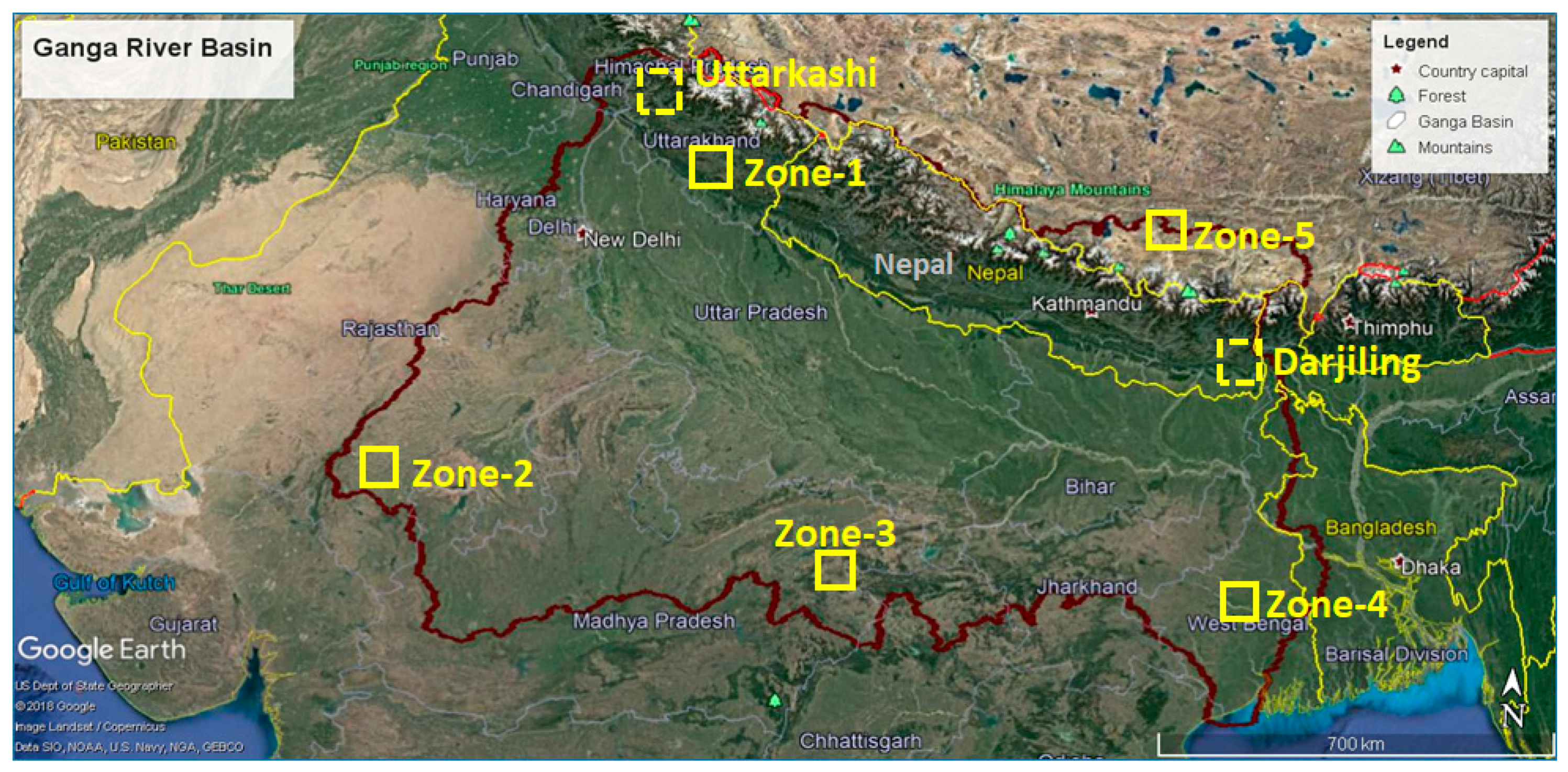
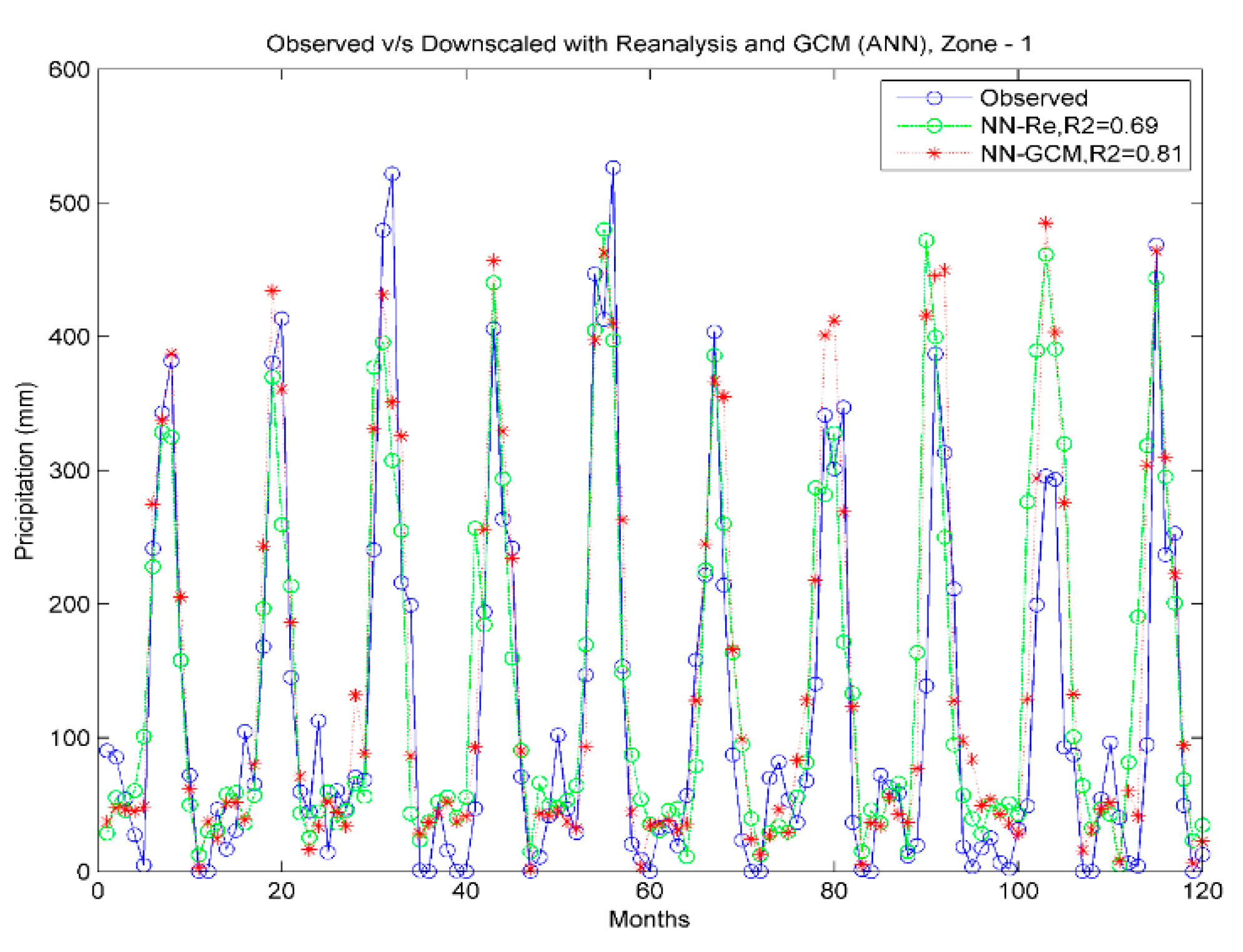
Re-Obs and GCM-Obs models were used to downscale historical GCM data at each grid point of zones 1 to 5, in the Uttarakhand and Darjeeling districts. Downscaled precipitation using both models were compared with observed precipitation for the model performance assessment. Zonal averaged values of observed and downscaled precipitation were considered for comparison in each zone. Time series of observed and downscaled precipitation by the Re-Obs model with CMCC-CMS GCM and the GCM-Obs model with GFDL-CM3 GCM for zone 1 and the Darjeeling district is shown in Figure 6 and Figure 7, respectively. A considerable difference in downscaled precipitation when using Re-Obs and models can be observed. The coefficient of determination (R²) between observed and downscaled precipitation by Re-Obs and GCM-Obs models varies from 0.5 to 0.69 and 0.8 to 0.81, respectively. Higher variability between observed and downscaled precipitation can be seen by with the Re-Obs model than with the GCM-Obs model for Darjeeling. Similar results were also found for other regions.

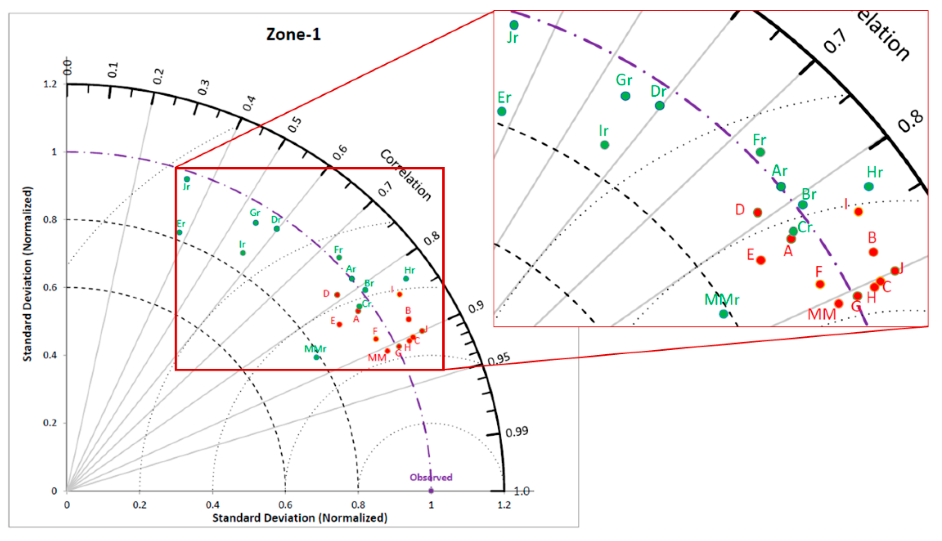
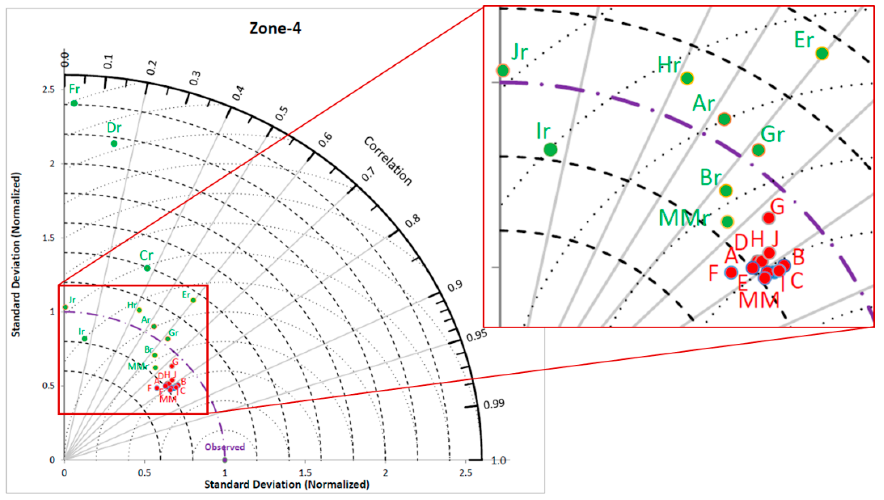
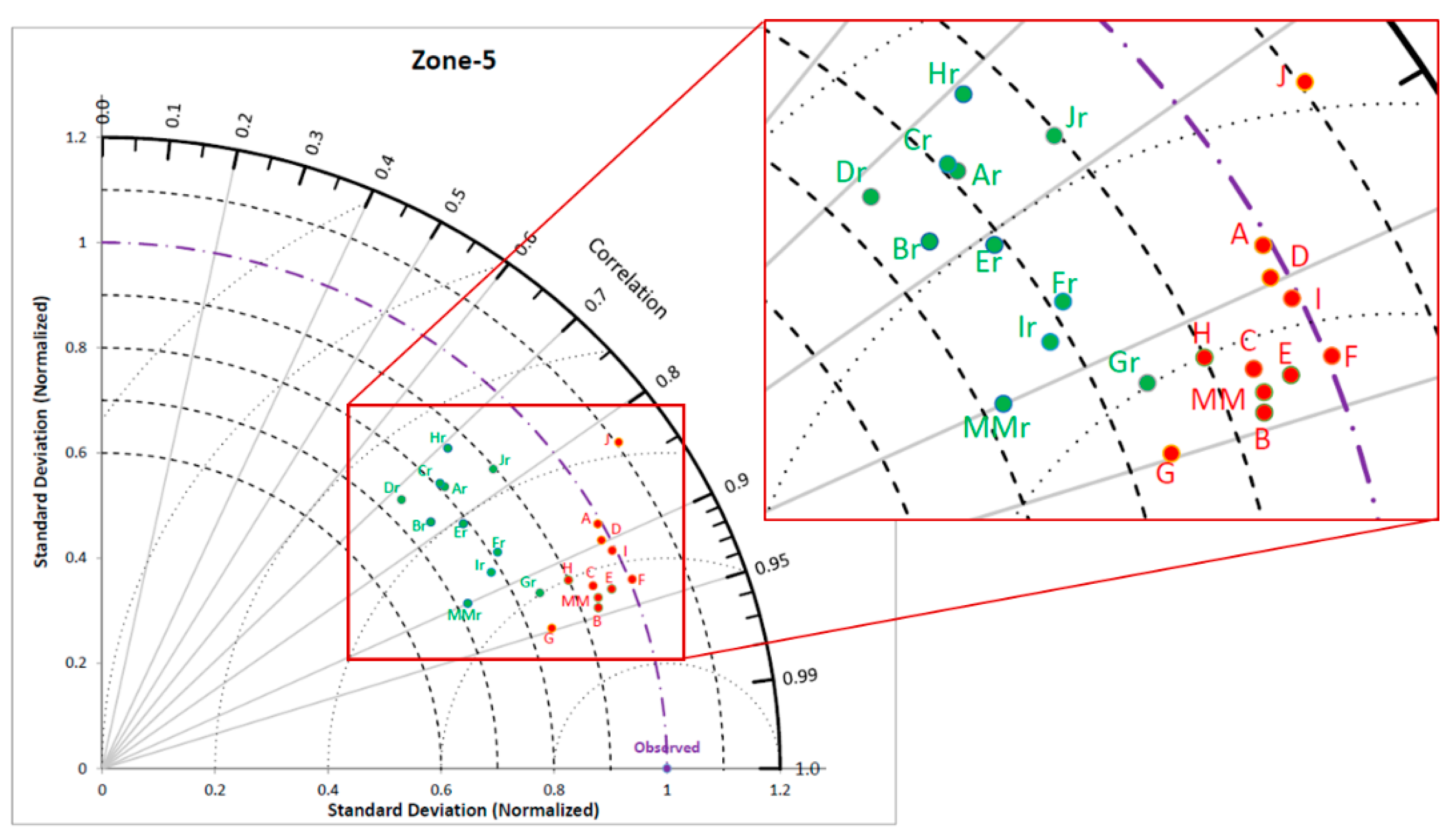
Along with a comparison of downscaling performance by both models for zone-1 to 5, Uttarkashi and Darjeeling districts are also represented by Taylor diagrams [56] in Figure 8, Figure 9, Figure 10, Figure 11, Figure 12 and Figure 13, respectively. A Taylor diagram is a useful plot to concisely show the degree of similarity between observed and modeled data. In this study, a Taylor diagram is used to show the relative performances of both methods to downscale precipitation with different GCMs. Radial lines from origin show the correlation between observed and downscaled precipitation. X and Y axis indicate the normalized standard deviation, which is computed by the following formula:

$$Normalizedstandarddeviation\left(NSD\right)=\frac{\mathrm{Standard}\mathrm{deviation}\mathrm{of}\mathrm{downscaled}\mathrm{precipitaion}}{\mathrm{Standard}\mathrm{deviation}\mathrm{of}\mathrm{observed}\mathrm{precipitation}}$$

(35)

NSDs are represented by two sets of concentric arches of circles having centers at origin and observed data point. NSD and correlation coefficient for observed data is always unity and marked at unit correlation and unit NSD in Taylor diagrams. Points in green and red colour represent downscaled precipitation with Re-Obs and GCM-Obs models, respectively. GCM Multi-model ensemble averaged precipitation is also calculated by adding more weight to the highly correlated GCM downscaled precipitation with observed precipitation using the following formula.

$$\mathrm{M}{\mathrm{M}}_t={\left(\frac{{\displaystyle \sum _{i=1}^n{r}_{i}D{P}_i}}{{\displaystyle \sum _{i=1}^n{r}_i}}\right)}_t$$

(36)

Here, MM_t is the GCM Multi-model ensemble averaged precipitation at time t, $r_i$ is correlation between downscale precipitation (DP) and observed precipitation for particular GCM, i = 1, 2, …, n number of GCMs (here ‘n’ is 10).

Notations used in this study to represent precipitation downscaled by Re-Obs and GCM-Obs models with different GCMs are given in

Table 8. Notations used in study for downscaling with different GCMs by Re-Obs and GCM-Obs models.

S.N.	GCM/Observed	Notation for the Re-Obs Model	Notation for the GCM-Obs Model
1	CMCC-CESM	Ar	A
2	CMCC-CM	Br	B
3	CMCC-CMS	Cr	C
4	FGOALS-g2	Dr	D
5	FGOALS-s2	Er	E
6	GFDL-CM3	Fr	F
7	HadGEM-AO	Gr	G
8	INMCM4	Hr	H
9	MIROC-ESM	Ir	I
10	MIROC-ESM-CHEM	Jr	J
11	Multi-model ensemble average	MMr	MM
12	Observed	Obs	Obs

.

Figure 8 shows the Taylor diagram for zone 1. Downscaled precipitation determined by the Re-Obs model with MIROC-ESM-CHEM and FGOALS-s2 GCMs is found to be the least correlated with observed precipitation, as it has a correlation coefficient (r) of 0.36 and 0.38 respectively. The GCM-Obs model is showing a significant improvement in similarity of downscaled precipitation with observed precipitation compared to the Re-Obs model. The coefficient of correlation improved to 0.9 and 0.83 using the GCM-Obs model with MIROC-ESM-CHEM and FGOALS-s2 GCMs, respectively. 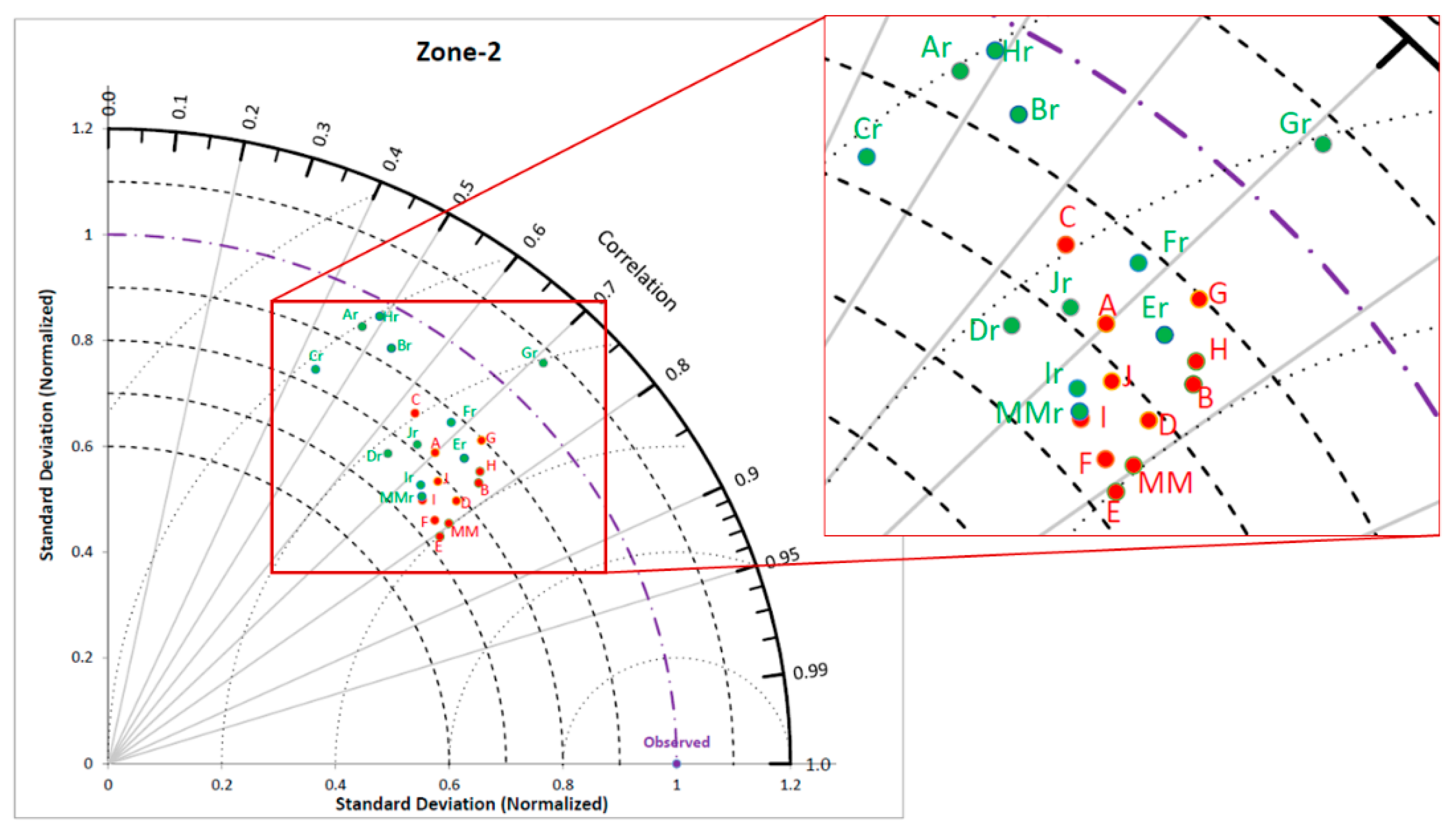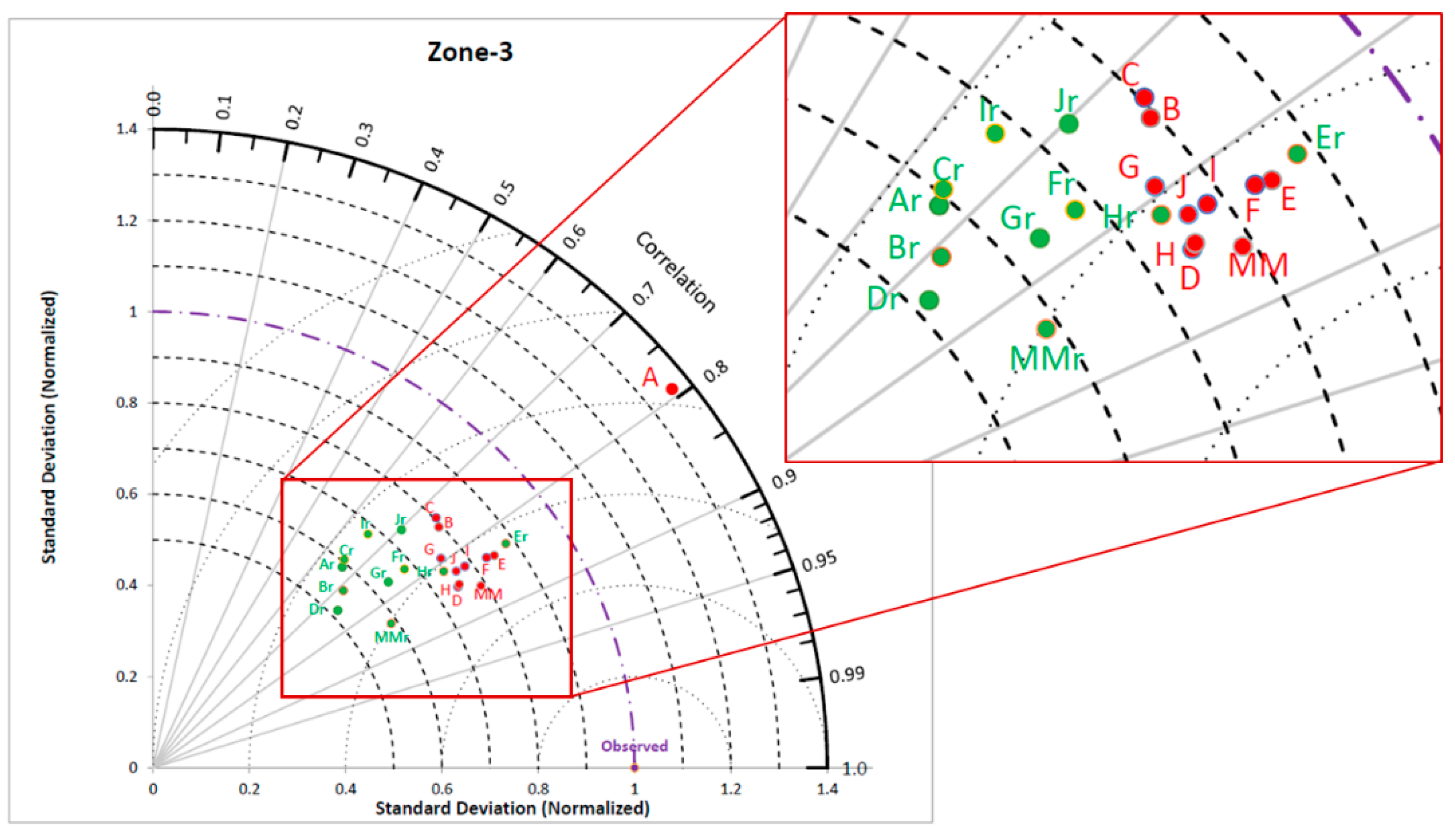NSD values by the GCM-Obs model are considerably better than the Re-Obs model, which shows less bias in observed and GCM downscaled precipitation. Similarly, Taylor diagrams for zone 2 to 5 also show improved similarity in downscaled precipitation by the GCM-Obs model than the Re-Obs model. 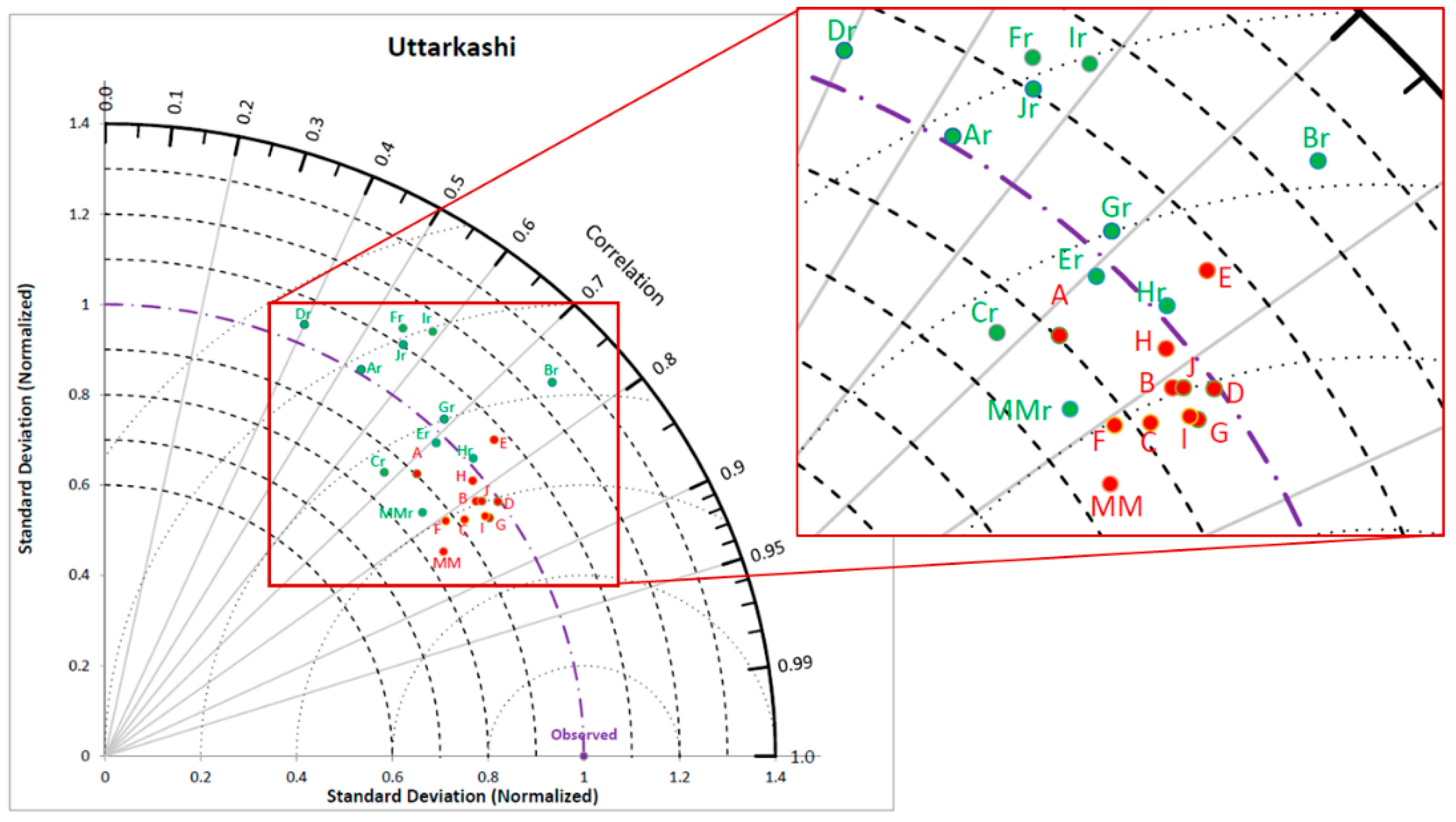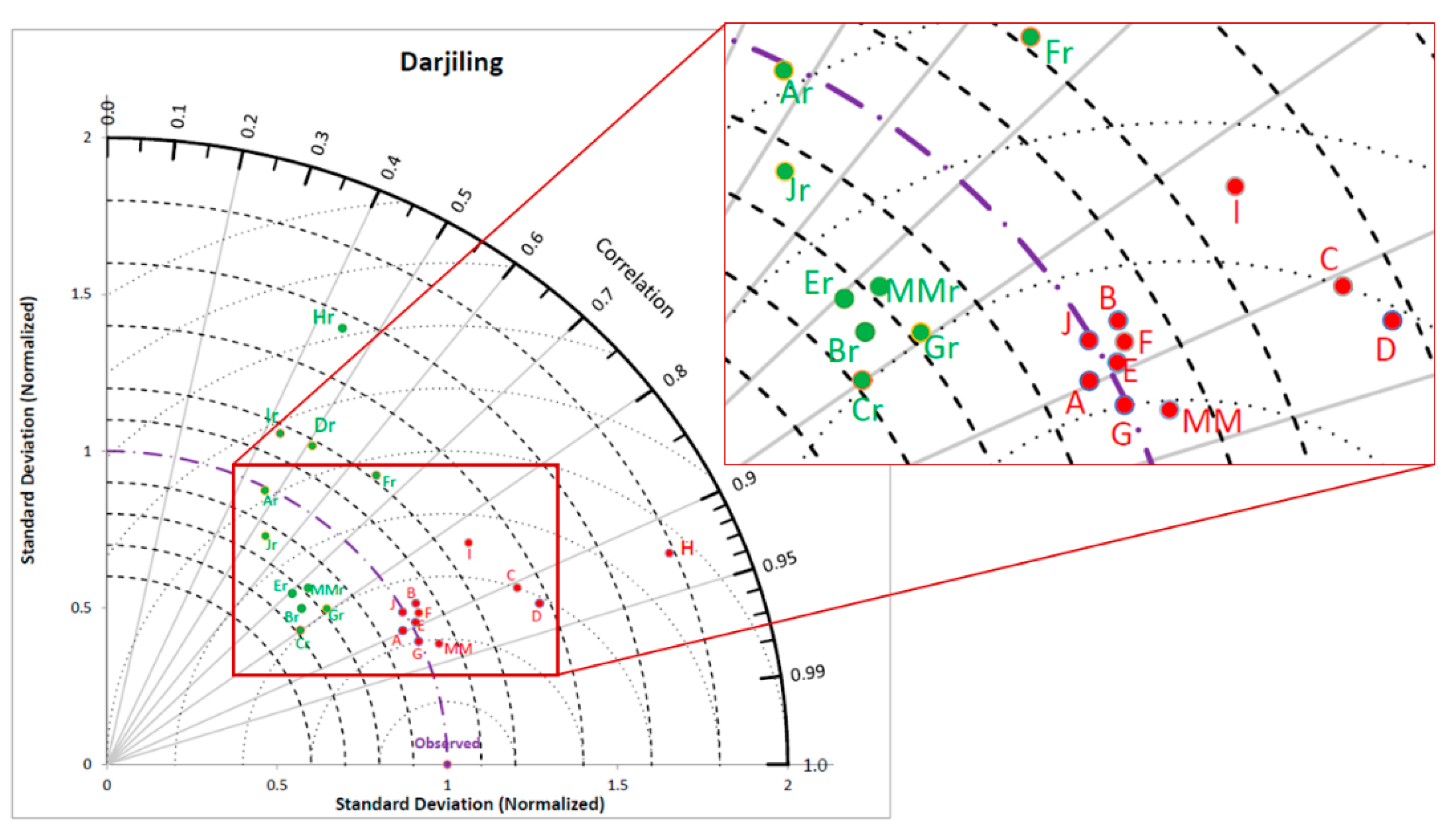Figure 13 and Figure 14 represent the Taylor diagram for district Uttarakhand and Darjeeling, respectively, for which IWP observed data was used. Figure 13 and Figure 14 also show more significant improvements in downscaled precipitation with the GCM-Obs model than with the Re-Obs model. Taylor diagrams for most of the study area show that downscaled precipitation in the GCM-Obs model with a different GCM is in the form of cluster.

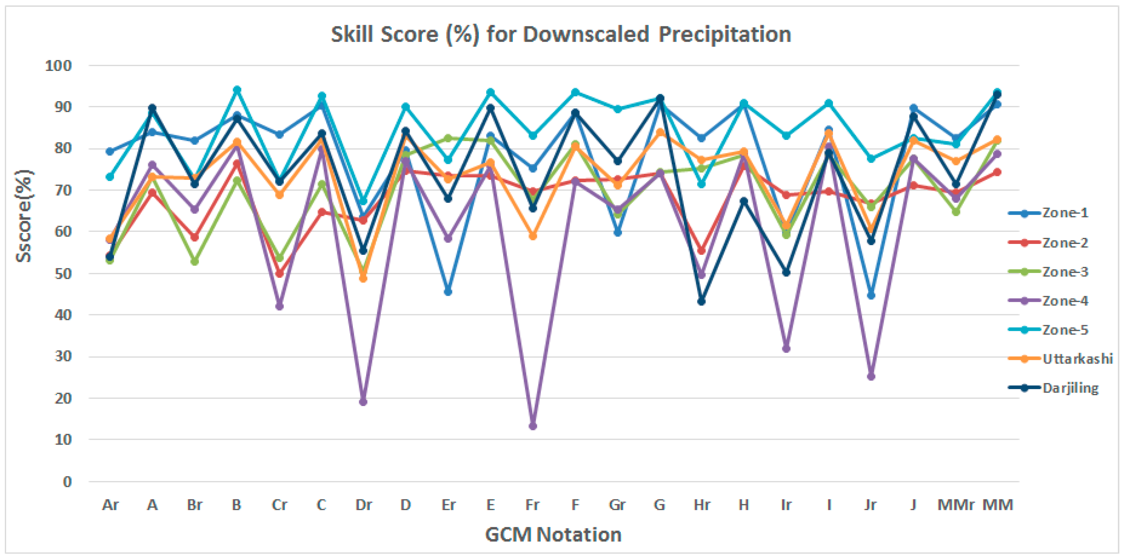
Skill score [56] is a popular method used to check the skill of model to simulate the results close to target data. Skill score increases with increase in correlation between simulated and observed data. It also increases when variance of modeled data approaches near to observed data. Skill score is defined as follows:

$$S_{score}(\%)=\frac{4{(1+\mathrm{R})}^K}{{(\sigma +\raisebox{1ex}{$1$}\!\left/ \!\raisebox{-1ex}{$\sigma $}\right.)}^2{(1+R_0)}^K}\times 100$$

(37)

Here, R is correlation between modeled and observed series, $\sigma$ is the ratio of standard deviation of modeled and observed series, K is a penalty parameter imposed for low correlation (here K = 2) and $R_0$ is maximum possible correlation which is assumed to be unity here.

The skill score of downscaled precipitation by Re-Obs and GCM-Obs models with different GCMs is shown in Figure 15. Peaks and troughs are visible in the plot, where downscaled precipitation by GCM-Obs and Re-Obs models are at peaks and troughs, respectively. Skill scores by the GCM-Obs model vary from 65% to 95% and 15% to 80% with the Re-Obs model. Zone 4 shows the least skill score under the Re-Obs model, which improved significantly by using the GCM-Obs model.

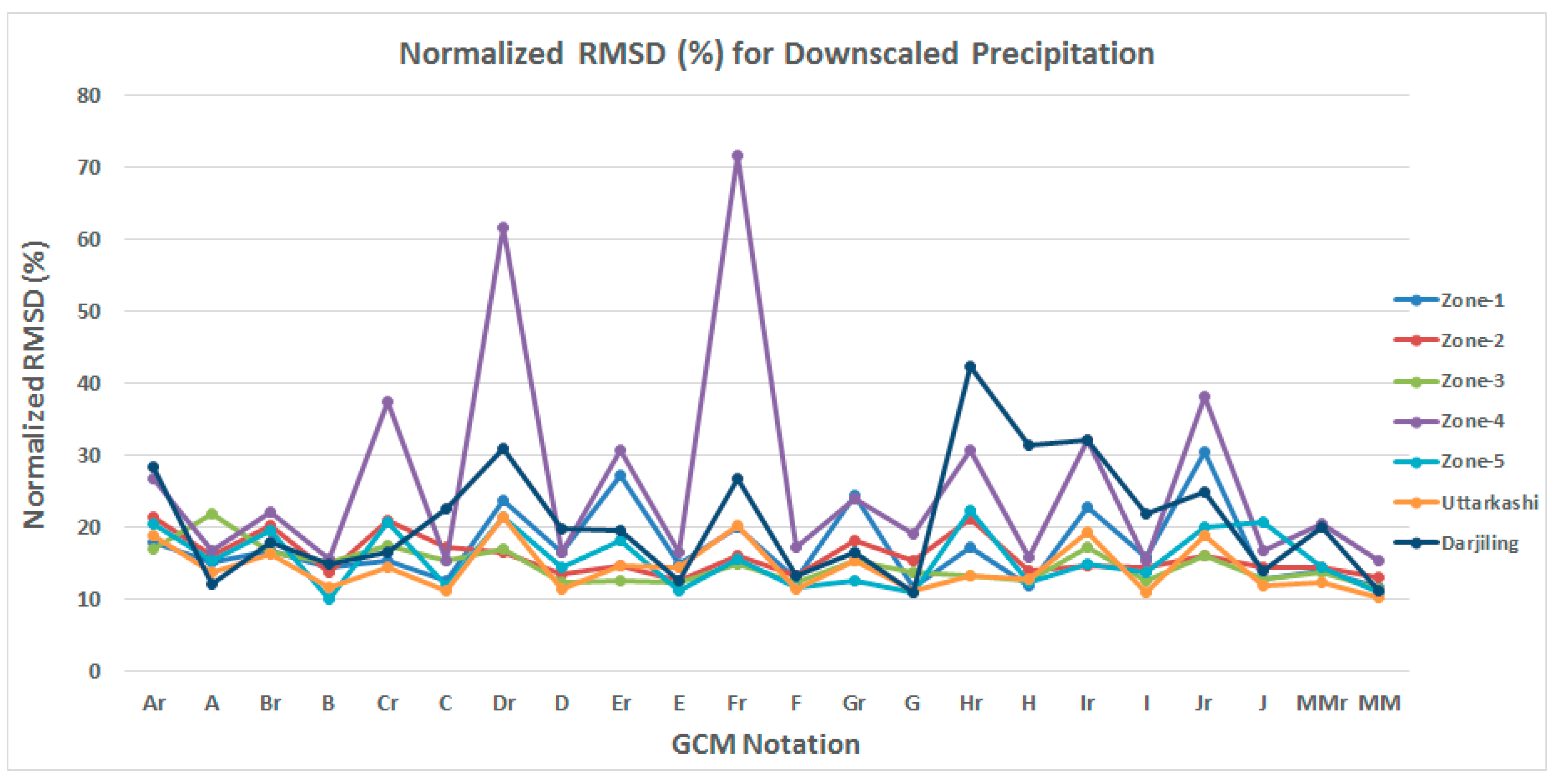
Root Mean Square Deviation (RMSD) is also a good measure to assess the predictive power of model. It directly relates difference between modeled and target data considering each data point. Lower values of RMSD shows better matching between modeled and target data. RMSD is generally presented in a normalized form to remove the scale difference between different data sets. The following formula is used to calculate a normalized RMSD.

$$NRMSD(\%)=\frac{1}{\left({\theta }_{\max }-{\theta }_{\min }\right)}\sqrt{\frac{{\displaystyle \sum _{t=1}^N{\left({\theta }_t-\widehat{{\theta }_t}\right)}^2}}{N}}\times 100$$

(38)

Here, ${\theta }_t$ and $\widehat{{\theta }_t}$ are observed and simulated values at time t, t = 1, 2, …, N number of months, ${\theta }_{\max }$ and ${\theta }_{\min }$ are maximum and minimum values of respective observed series.

NRMSD of downscaled precipitation with different GCMs by Re-Obs and GCM-Obs models is shown in Figure 16. Downscaled precipitation by the Re-Obs model at peaks and by the GCM-Obs model at troughs in the plot clearly shows the improvement in the closeness of downscaled data with observed data. FGOALS-g2, GFDL-CM3 and INMCM4 GCMs show comparatively higher NRMSD.

Performance of the GCM-Obs model was found to be better than the Re-Obs model in downscaling precipitation in close range of observed precipitation following similar patterns. Different measures adopted to check the performance of both models indicate the high performance of the GCM-Obs model over the Re-Obs model in measuring downscale precipitation with different GCMs.

Two measures are adopted to show convergence skill of both models (i) correlation matrix and (ii) NRMSD matrix. These measures are discussed in detail in following paragraphs.

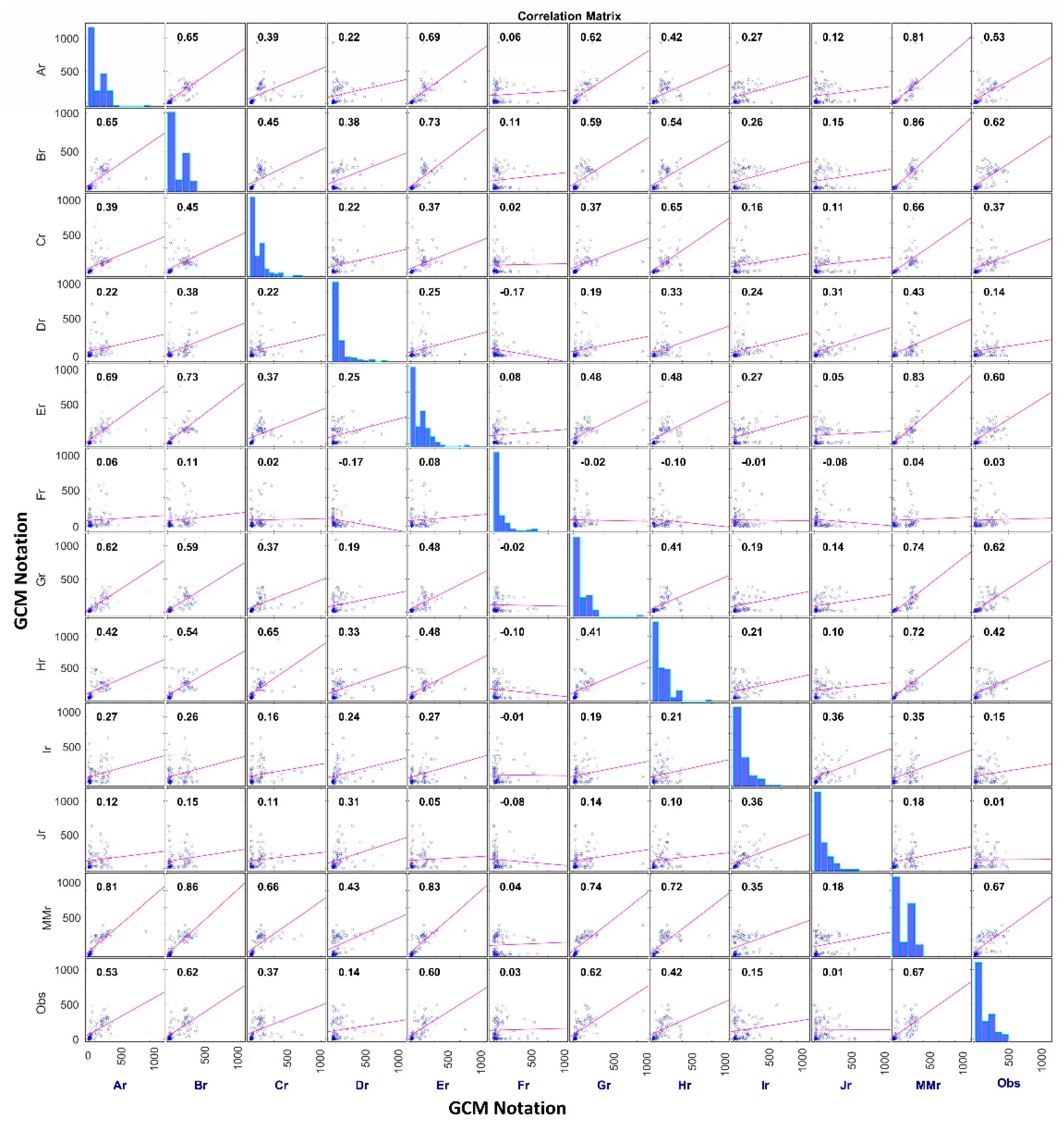
Correlation coefficient (r) is a good measure to check linear similarity between two datasets. Higher value of r shows higher similarity. The Pearson correlation coefficient is adopted in this study, which is computed as follows:

$$r_{X,Y}=\frac{{\displaystyle \sum _{t=1}^N\left(x_t-\overline{x}\right){\displaystyle \sum _{t=1}^N\left(y_t-\overline{y}\right)}}}{\sqrt{{\displaystyle \sum _{t=1}^N{\left(x_t-\overline{x}\right)}^2}}\sqrt{{\displaystyle \sum _{t=1}^N{\left(y_t-\overline{y}\right)}^2}}}$$

(39)

Here, $r_{X,Y}$ is Pearson correlation coefficient between datasets $X$ and $Y$, $\overline{x}$ and $\overline{y}$ are mean of datasets $X$ and $Y$ respectively, $x_t$ and $y_t$ are values of datasets at time t = 1, 2, …, N.

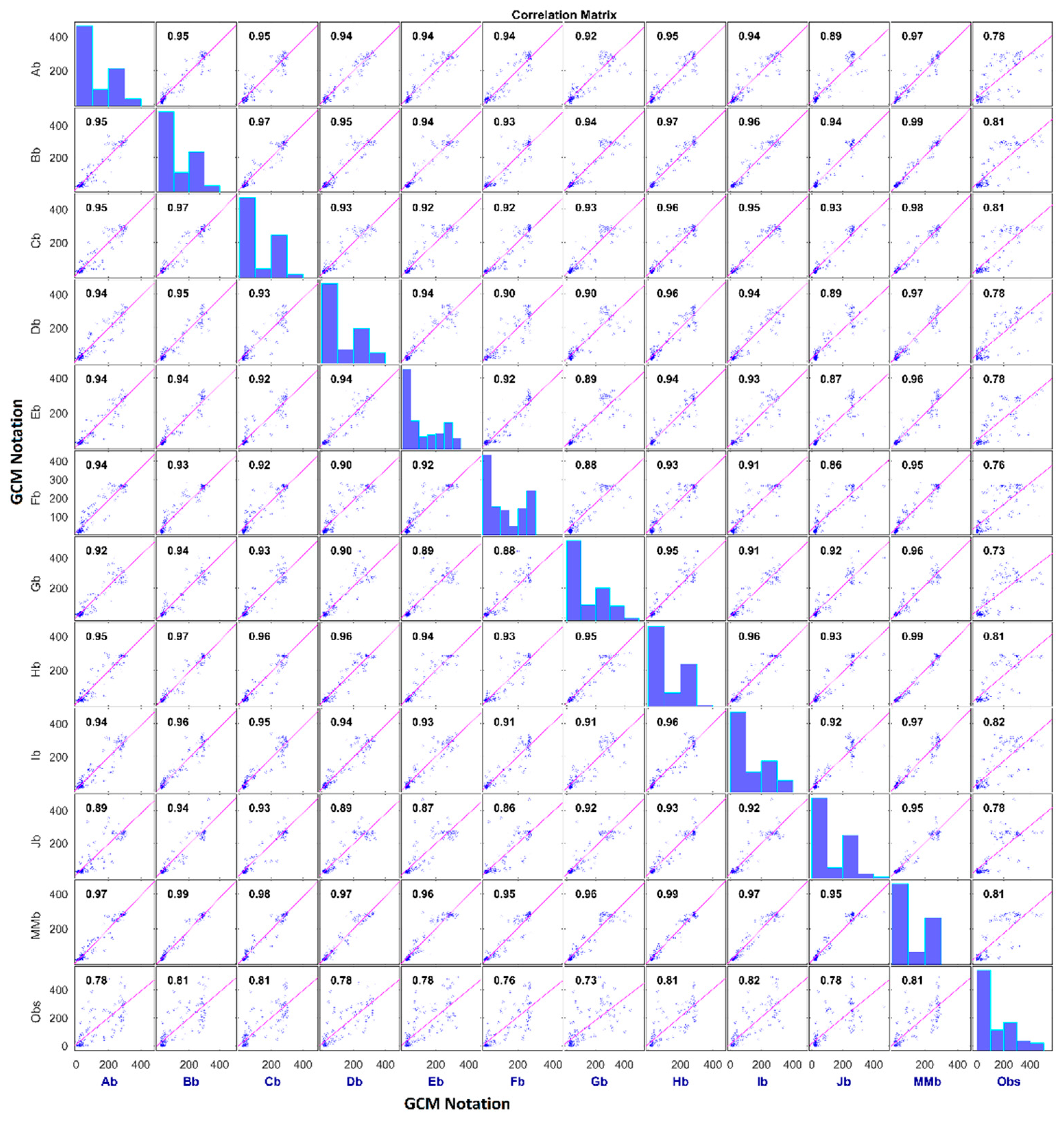
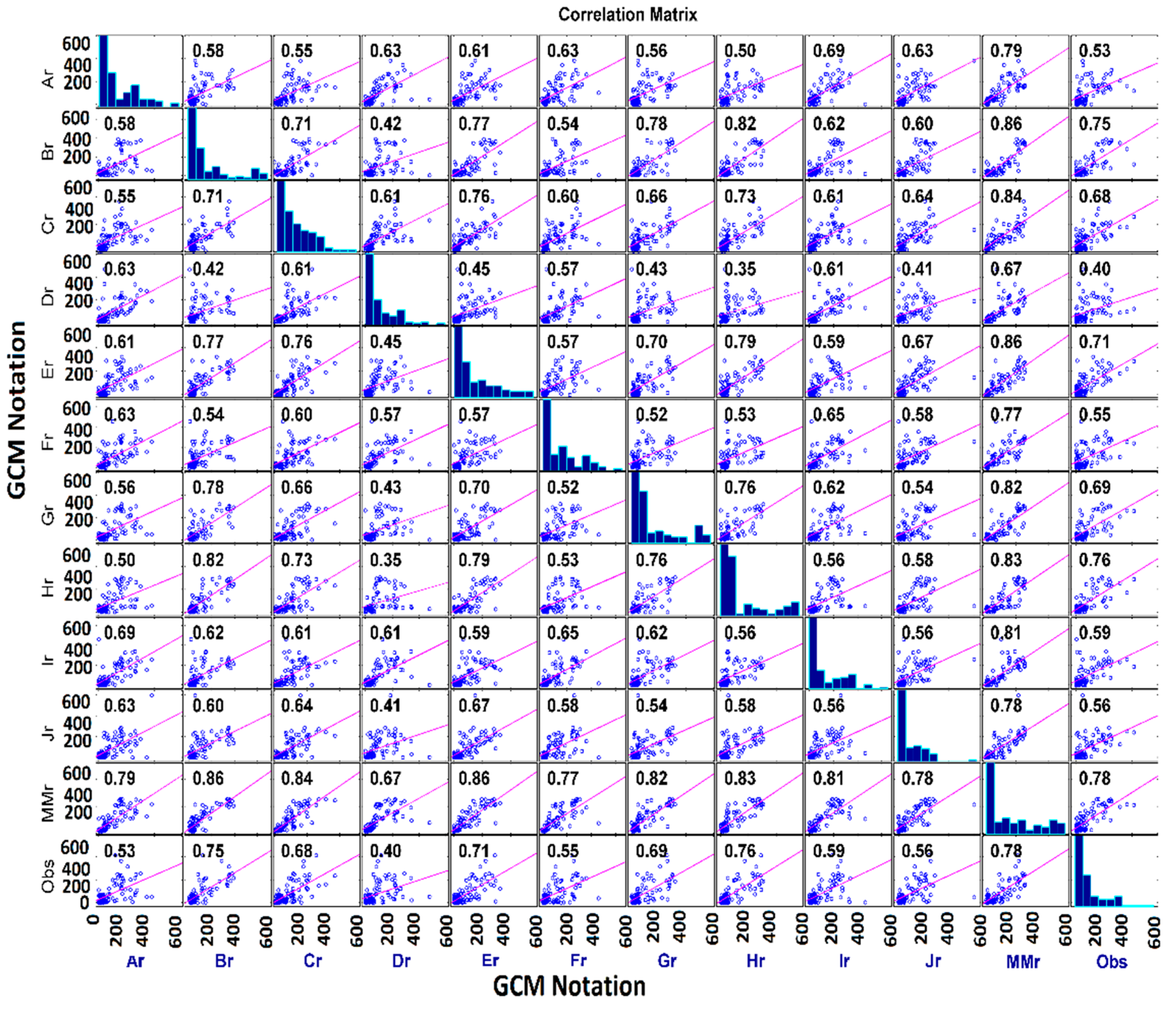
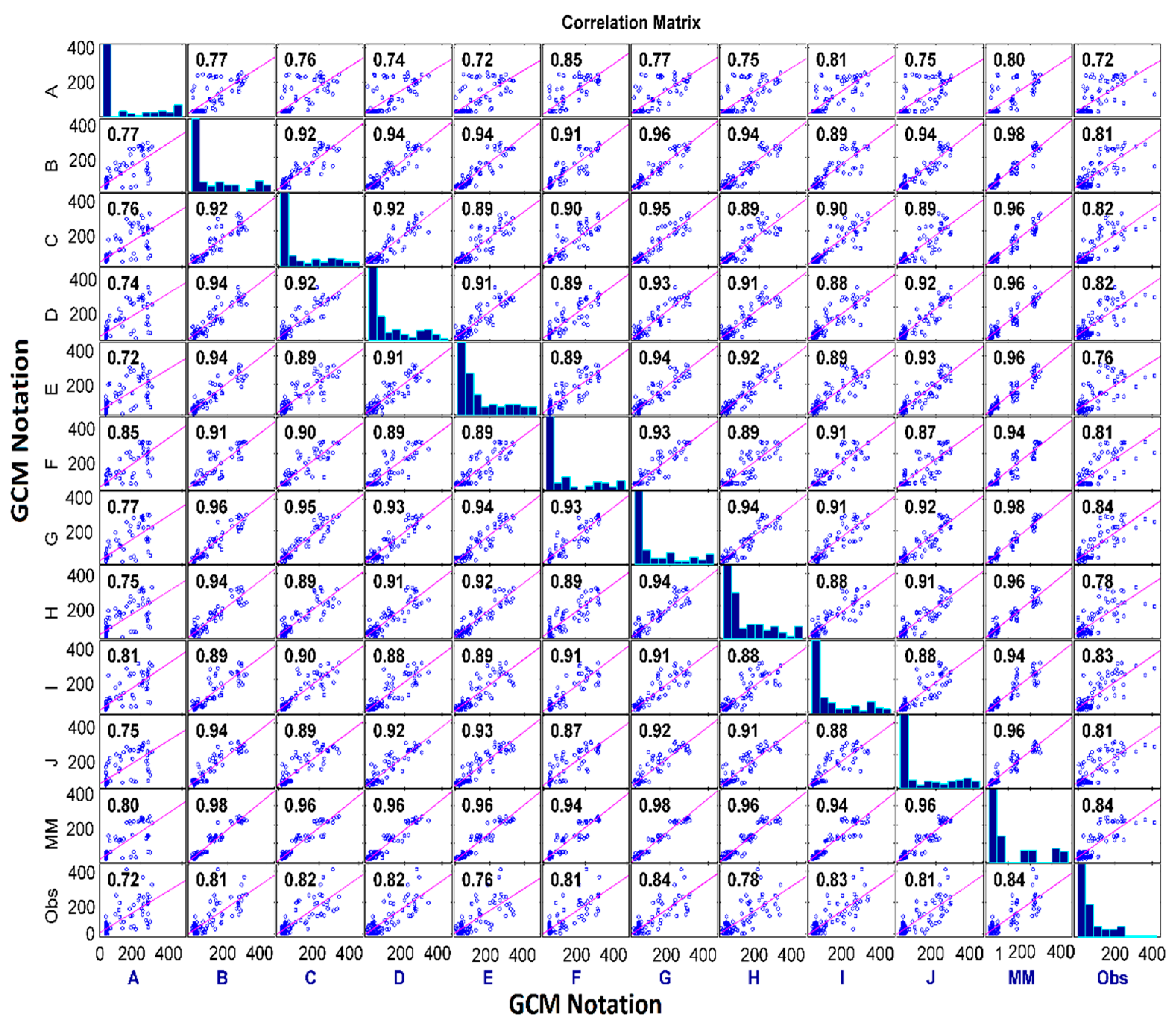
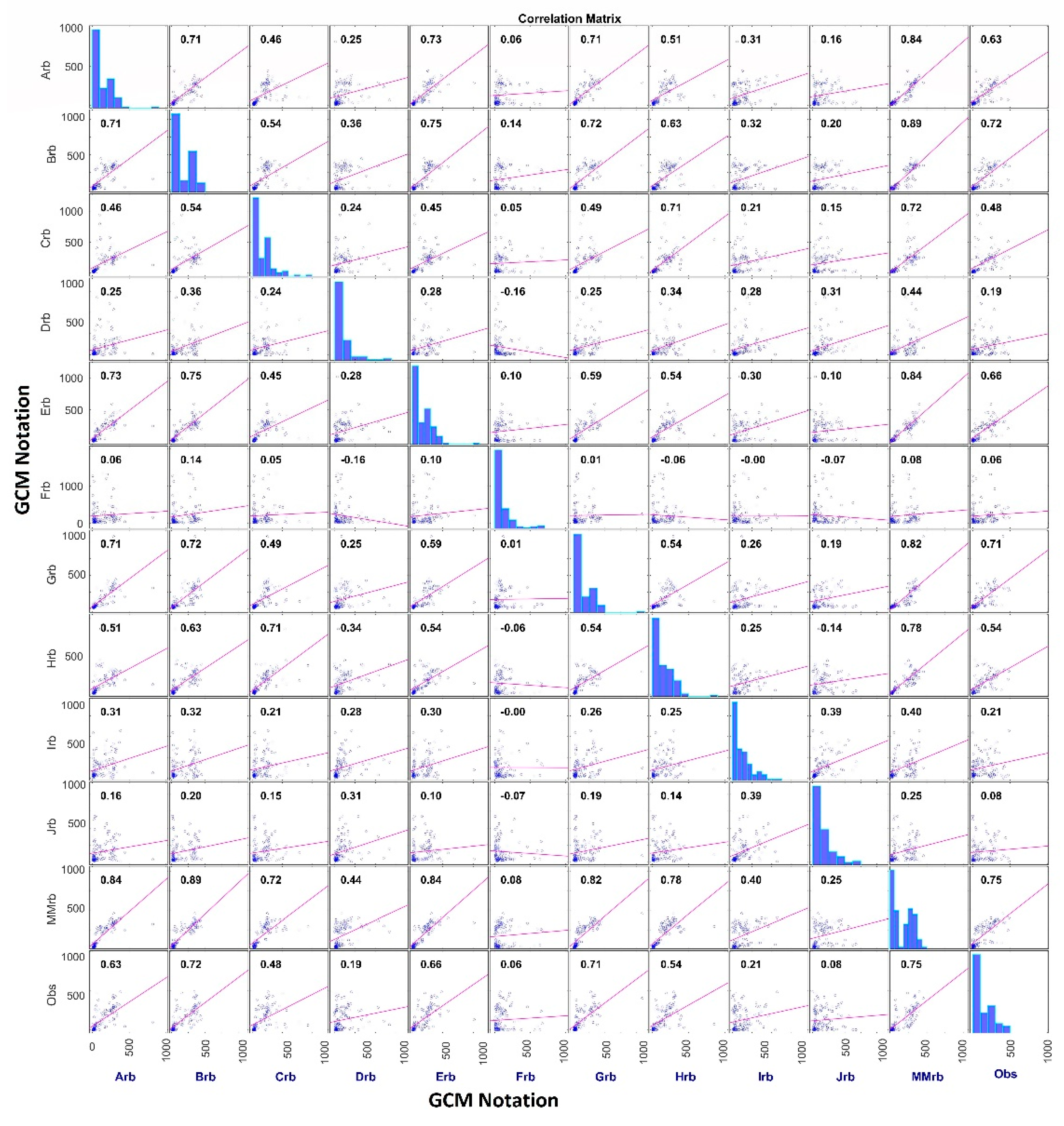
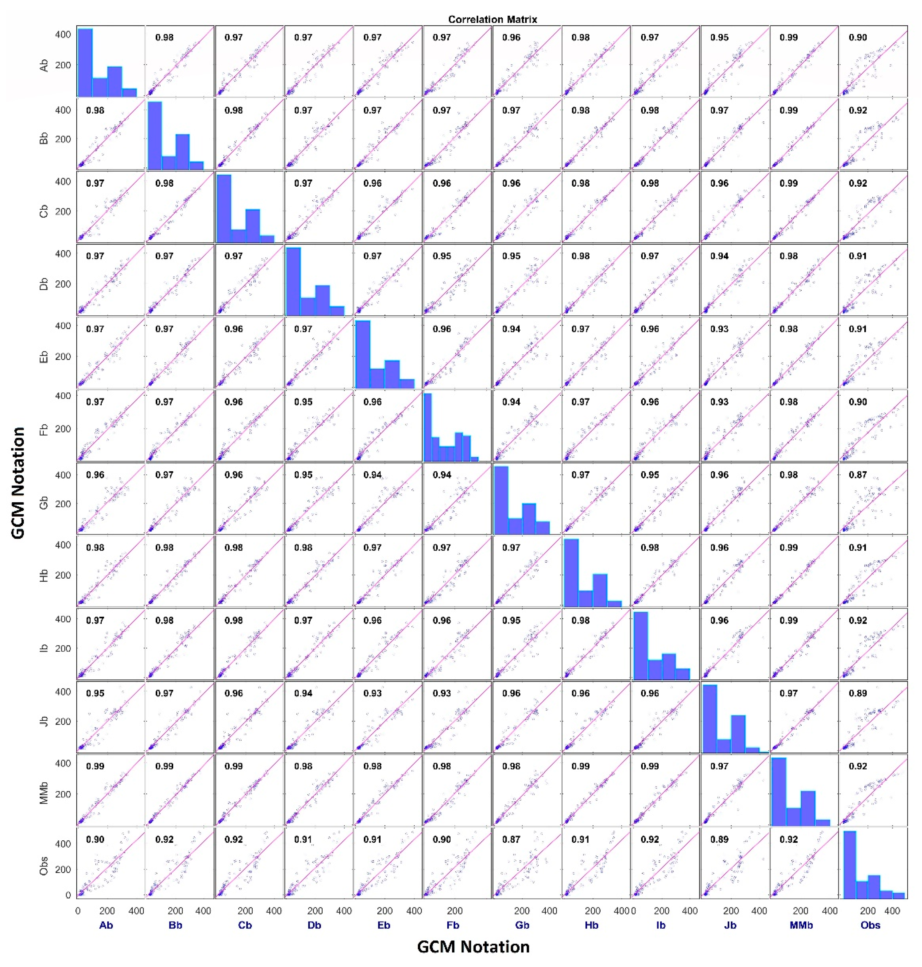
Correlation coefficient between downscaled precipitation with different GCMs by the Re-Obs and GCM-Obs models are presented in the form of a correlation matrix. Correlation between downscaled and observed precipitation is also shown. The diagonal of the correlation matrix shows a histogram of respective data series. The correlation matrix of downscaled precipitation for zone 4 by the Re-Obs and GCM-Obs models is shown in Figure 17 and Figure 18 respectively. Similar matrix is also shown for Uttarkashi district in Figure 19 and Figure 20.

A correlation matrix with the Re-Obs model for zone 4 and Uttarkashi shows a significant difference in downscaled precipitation. Four GCMs, i.e., FGOALS-g2, GFDL-CM3, MIROC-ESM and MIROC-ESM-CHEM, show almost no correlation with other GCMs, the Multi-model ensemble average, and observed data. A correlation matrix involving the GCM-Obs model shows a significant improvement in the correlation between GCMs. GCMs shows high correlation among themselves with a correlation coefficient of 0.88 to 0.97 with the GCM-Obs model instead of almost 0 to 0.73 with the Re-Obs model. This shows a significant reduction in GCM-GCM bias. Similar results were also found for other regions.

NRMSD was again used to judge the convergence skill of both models in downscaled precipitation with different GCMs. To show the closeness of downscaled precipitation with different GCMs under the Re-Obs and GCM-Obs models, a NRMSD matrix is prepared as follows:

$${\left(NRMSD\right)}_{X,Y}(\%)=\frac{1}{\left({\theta }_{\mathrm{obs}\_\max }-{\theta }_{\mathrm{obs}\_\min }\right)}\sqrt{\frac{{\displaystyle \sum _{t=1}^N{\left({\theta }_{\mathrm{X},t}-{\theta }_{\mathrm{Y},t}\right)}^2}}{N}}\times 100$$

(40)

Here, ${\left(NRMSD\right)}_{X,Y}$ is normalized root mean square deviation between downscaled precipitation for $GC{M}_X$ and $GC{M}_Y$, X, Y = 1, 2, …, 10, ${\theta }_{\mathrm{X},t}$ and ${\theta }_{\mathrm{Y},t}$ are downscaled precipitation of $GC{M}_X$ and $GC{M}_Y$ at time t, t = 1, 2, …, N number of months, ${\theta }_{\mathrm{obs}\_\max }$ and ${\theta }_{\mathrm{obs}\_\min }$ is maximum and minimum observed precipitation respectively.

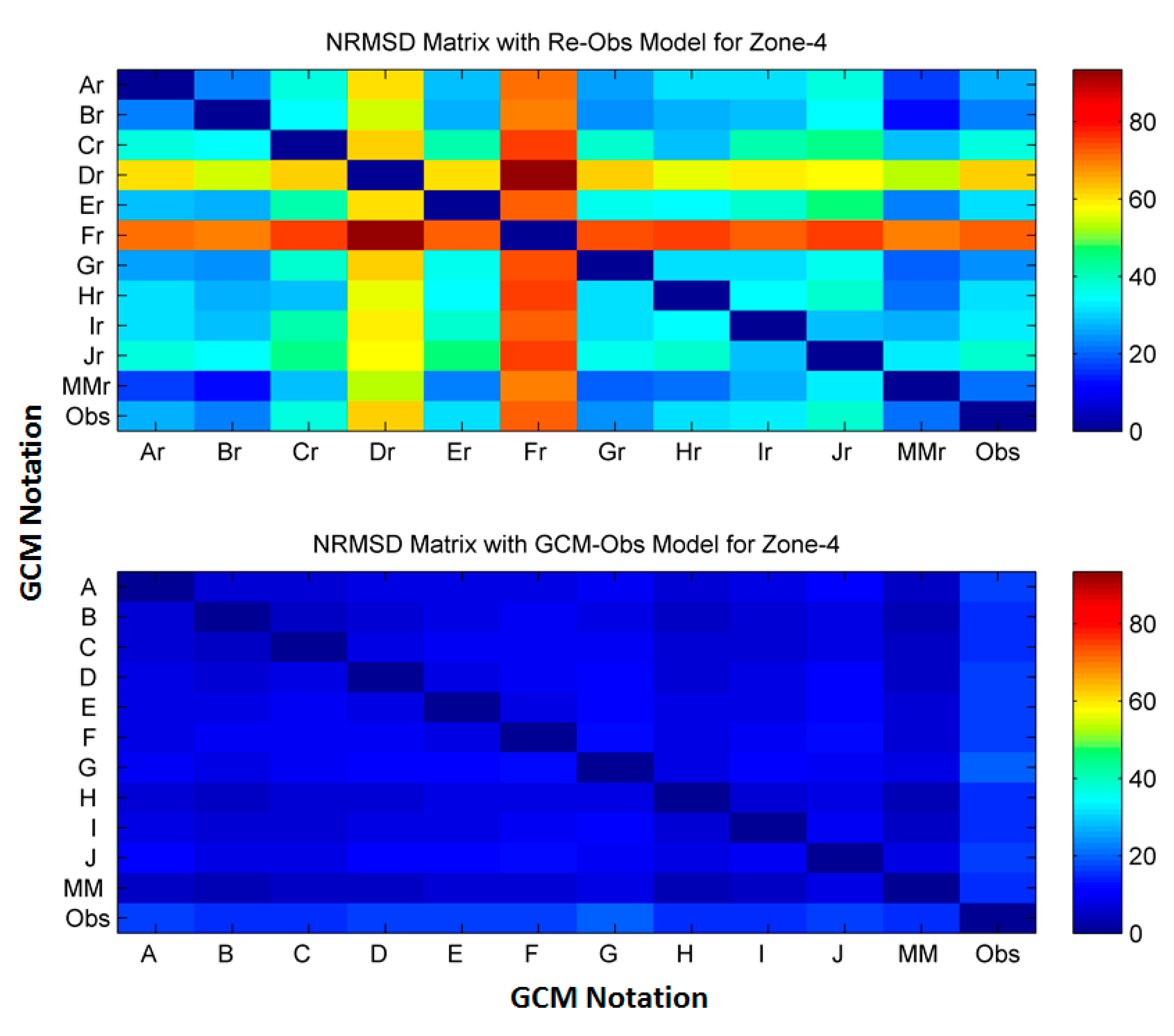
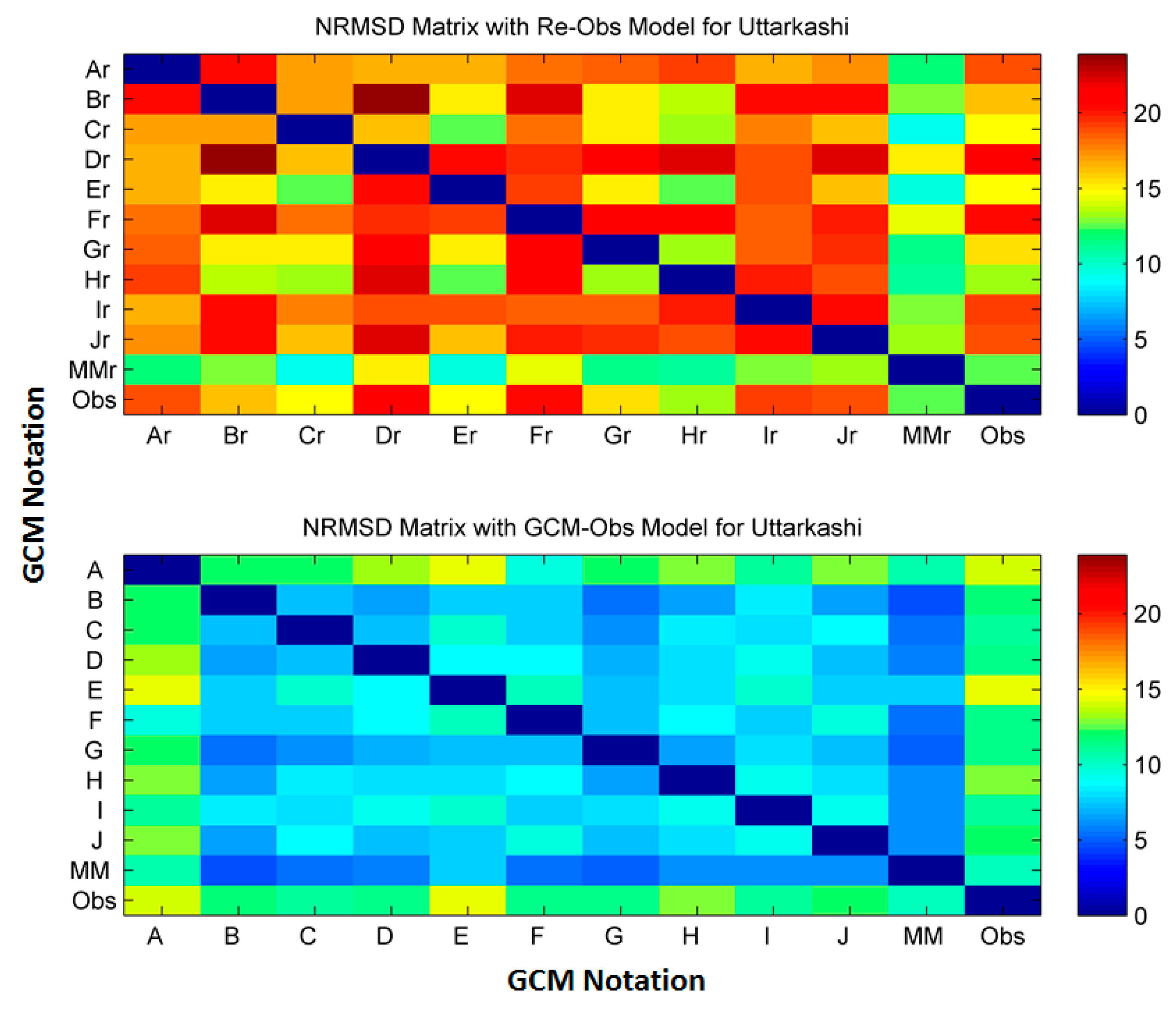
The pattern of the NRMSD matrix of downscaled precipitation by both models for Zone 4 and Uttarkashi are shown in Figure 21 and Figure 22, respectively. Two GCMs, i.e., FGOALS-g2 and GFDL-CM3, downscaled by the Re-Obs model show the highest variability with other GCMs and observed data for Zone 4 and Uttarkashi. The NRMSD value of the order of 70%–90% with the Re-Obs model is significantly reduced to 5%–15% by the GCM-Obs model for zone 4. Similarly, for Uttarkashi, the NRMSD of 15%–30% using Re-Obs model is reduced to 5–15% using GCM-Obs model. A significant reduction in the NRMSD value can also be seen with observed data using the GCM-Obs model. It can also be seen that the spatial resolution of GCM is not an influencing parameter in downscaling. A mixed pattern of downscaling performance is achieved on downscaling using coarser gridded CMCC-CESM to obtain relatively finer gridded CMCC-CM GCMs. Similar results were also found for other regions.

It can be noted from the results above that the GCM-Obs model performs better than the Re-Obs model in statistical downscaling. However, bias correction methods are generally adopted with the Re-Obs model to reduce GCM bias. Lie et al. [32] proposed Equidistant CDF matching (EDCDFm) bias correction method which is widely used to correct bias in monthly precipitation and temperature. The same method is used to correct the bias in downscaled precipitation using the Re-Obs and GCM-Obs models. 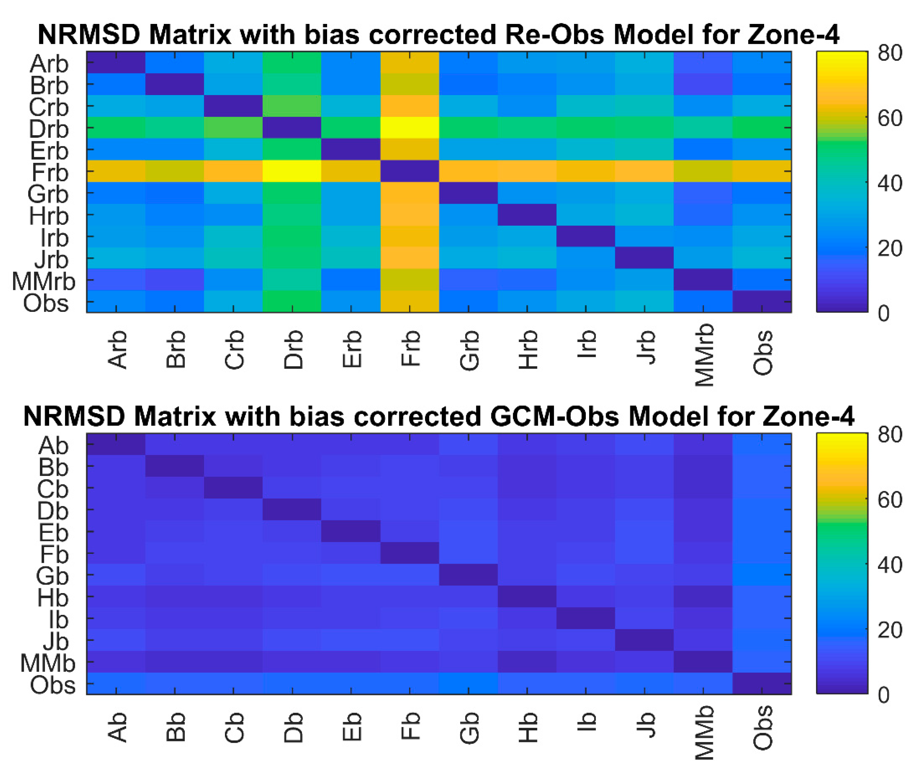The performance of both models considering EDCDFm bias correction method for zone-4 is presented by NRMSD matrix and correlation plots.

The correlation matrix for the bias corrected Re-Obs and GCM-Obs are shown in Figure 23 and Figure 24, respectively. It can be observed from the Figure 17 and Figure 23 that the bias correction method improved the downscaled precipitation. However, bias correction also improved the downscaled precipitation using the GCM-Obs model. So, the bias correction method improved the inter GCM and GCM-observed correlation and the GCM-Obs model performed better than the Re-Obs model.

The NRMSD matrix of bias corrected downscaled precipitation using Re-Obs and GCM-Obs models is shown in Figure 25. Here also, the bias correction method improved the downscaling performance of both models, and the GCM-Obs model was found to be better than the Re-Obs model.

Measures adopted to judge the convergence skill of both models indicate the GCM-Obs model’s capability to reduce GCM bias, and show a better convergence skill than the Re-Obs model with or without using bias correction methods. Overall, it can be conveyed that the GCM-Obs model performs better than the Re-Obs model.

5. Discussion

This article discusses the choice of a better statistical downscaling model among Re-Obs and GCM-Obs to downscale GCM data. The former Re-Obs model is adopted by the majority of researchers. However, the bias in the GCM downscaled product from observations and the differences in GCM downscaled product using different GCMs is major concern of the climate researchers [8,15,21]. The Re-Obs and GCM-Obs models are compared using three methods: (i) Mathematical derivation, (ii) Synthetic Series and (iii) a case study considering real observed data. The Performance of the GCM-Obs model was found to be better than the Re-Obs model for statistically downscaling GCM data. It may be argued that if the reanalysis data is closer to the observed data, it should be able to better downscale GCM, but the Re-Obs model could produce better results if the reanalysis products are to be downscaled. However, if the goal is to downscale GCM, the obvious choice for the predictor -predictand model should be the GCM-Obs model, as it already considers the characteristics of the GCM that will be downscaled.

The performance of Re-Obs and the GCM-Obs model for statistically downscaling precipitation in different regions in the Ganga river basin was checked using different skill scores [35,41]. The case study indicates that the GCM-Obs model could be better choice for statistically downscaling GCM. The GCM-Obs model can be used to downscale different CMIP5 experiments [57], as reported in the IPCC AR5 for assessing different climate states while considering different assumptions.

6. Limitations of the Study

The study aimed to propose a different downscaling approach to improve the similarity of the downscaled variable and observed data and to reduce variability in downscaled data using different GCMs. Downscaling can be further improved by using a different set of predictor variables, downscaling methods, and other techniques/methods. In this study ten different GCMs are considered and the results can be verified with other GCMs as well. However, the results are likely to be in agreement with this study. Uncertainty is inherent with GCM due to different boundary conditions, equations, methods and other factors in the development of different GCMs. GCM uncertainty cannot be fully removed, but in this study an effort has been made to reduce the variability in downscaled variables using a different downscaling approach. Observed data is obtained from renowned agencies which take utmost care in sampling and production in datasets, but still errors in the data cannot be fully ruled out.

7. Conclusions

Statistical downscaling of precipitation in different regions in the Ganga river basin was carried out with ten different GCMs along with the Re-Obs and GCM-Obs models. The predictor-predictand relationship used to downscale GCM at a local scale was developed using reanalysis and historical GCM data as predictors in Re-Obs and GCM-Obs models, respectively. Different measures were adopted to judge the relative performances of Re-Obs and GCM-Obs models to downscale precipitation with different GCMs.

Downscaled precipitation with different GCMs by the Re-Obs and GCM-Obs models showed significant differences in each region of the study area. Although the predictor-predictor model showed good connection between reanalysis and observed data, but same model could not better simulate the downscaling of GCM. Higher variance and lesser correlation between modeled and observed precipitation was shown by the Re-Obs model. Development of the predictor-predictand relationship with historical data of GCM itself as the predictor and observed data as the predictand showed a high similarity and less variability in downscaled and observed precipitation. The skill score of downscaled precipitation also showed a more significant improvement with the GCM-Obs model than with the Re-Obs model. Datasets of downscaled precipitation with different GCMs using the GCM-Obs model fall near to each other in the form of clusters, as represented by the Taylor diagram.

Intercomparison of downscaled precipitation with different GCMs by the Re-Obs model also showed higher GCM-GCM bias, as indicated by the NRMSD correlation matrix. The GCM-Obs model significantly reduced GCM bias in downscaled precipitation for all regions and all GCMs. The GCM-Obs model showed its robustness in downscaling with different GCMs for all regions and both sets of observed data, i.e., GPCC and IWP. The GCM-Obs model was found to be more reliable in terms of performance and convergence skill than the Re-Obs model. Multi-model ensemble average precipitation data showed better resemblance with observed data than most of the individual GCM. It is also found that spatial resolution of the GCM does not have a considerable effect on performance and convergence skill for both models. The bias correction method also improves the downscaling performance of both Re-Obs and GCM-Obs.

It can be said that using historical GCM data to develop the predictor-predictand relationship is a better choice to simulate the precipitation and to reduce GCM uncertainty. The GCM-Obs model is robust against bias due to different data observing agencies. Predictor-predictand model development using historical data of GCM itself can be applied to downscale other atmospheric variables, i.e., temperature, humidity, evapotranspiration etc. Improvement in performance and reduction in GCM bias is also expected to downscale other variables under the GCM-Obs model, because precipitation is in least agreement with GCM in downscaling [58]. The bias correction measures may still be used to further improve the quality of the downscaled variable. This study will be helpful for climate change researchers to develop better downscaling models and to be more certain when they decide the ranges of downscaled atmospheric variables.