Dune Contribution to Flow Resistance in Alluvial Rivers


1
Department of Engineering, University of Ferrara, V. Saragat, 1, 44122 Ferrara, Italy
2
Department of Physics and Earth Science, University of Ferrara, 44122 Ferrara, Italy
3
International Platform for Dryland Research and Education, Tottori University, Tottori 680-8550, Japan
*
Author to whom correspondence should be addressed.
Water 2019, 11(10), 2094; https://doi.org/10.3390/w11102094
Submission received: 7 August 2019
/
Revised: 24 September 2019
/
Accepted: 1 October 2019
/
Published: 8 October 2019
(This article belongs to the Section Hydraulics and Hydrodynamics)
Abstract
:One of the most relevant features of alluvial rivers concerns flow resistance, which depends on many factors including, mainly grain resistance and form drag. For natural sand-bed rivers, dunes furnish the most significant contribution and this paper provides an insight on it. To achieve this aim, momentum balance equations and energy balance equations are applied to free flow in alluvial channels, assuming hydrostatic pressure distribution over the cross sections confining the control volume, which includes a reference bed form pattern. The resulting equation in terms of energy grade accounts for an empirical bed form drag coefficient resulting from the actual flow pattern and bed form geometry. The model has been validated using a large selection of field data and it seems somewhat sensitive to the dune geometry and to the Nikuradse equivalent roughness, whereas it is shows greater sensitivity to the adopted grain surface resistance formula (e.g., Manning–Strickler formula).
1. Introduction
In alluvial channels, flow resistance is the result of several factors, including the presence of bends, vegetation, local acceleration due to flow unsteadiness, and channel geometry variations, in addition to bed surface roughness and bed forms drag. Morphological evolution of active channels also affects flow resistance, since it is responsible for the evolution of large-scale bed forms (i.e., dunes and bars). Since the 1950s great efforts have been devoted to river morphodynamic models. Most of them consist of coupled systems of depth-averaged flow mass and momentum equations, a bed evolution equation, as well as a sediment transport formula. Valuable state-of-the-art technologies for river sedimentation and morphology modeling may be found in [1,2]. These conventional morphodynamic models mainly refer to nonlinear shallow water equations, Exner equation, and an empirical formula for sediment transport. Considerable uncertainty derives from the large number of such formulae available in the literature. Moreover, sediment transport in open channel flows includes bedload and suspended load; but, although different mechanisms govern these two modes of transport, a reliable method to account for both of them has not yet been provided [3]. In conventional models further uncertainty arises from the lack of understanding of some fundamental mechanics related to sediment transport. Among them, the effect of bed slope, which has been considered by Maldonado and Borthwick, who recently proposed a simplified two-layer model [4] for bedload-dominated scenarios. Alternatively, morphodynamic models based on two-phase and two-layer approaches may also be considered [5,6,7]. Although they are scientifically more insightful than the conventional approaches, they prove to be mathematically more complex and computationally more demanding.
Even in the case of steady and quasi-uniform flow, confined within the main active channel and involving non-cohesive sediment, most of the existing resistance formulae (e.g., [8,9,10,11]) commonly provide inaccurate predictions of flow resistance. This leads to considerable error in stage-discharge prediction, both in terms of water depth (±20%), flow velocity (±15%) [12] or bed friction, for which the difference between measured and predicted values may be ±50% [11] and, where field data is used, discrepancy is even wider [13,14]). Since the middle of the twentieth century this topic has attracted the interest of many scientists and several criteria-based methods have been proposed, based on linear and non-linear approaches.
In the latter case (e.g., [12,15,16,17]) the resistance coefficient is kept as a single factor and the method does not require any knowledge of bed form geometry (i.e., empirically-based approach). By contrast, the linear approach originally introduced by Meyer-Peter and Mueller [18] considers an overlapping of effects. In fact, flow resistance depends on forces acting on individual particles (i.e., skin friction) and on forces affected by bed form configuration (i.e., form drag). Among the others Azareh et al. [19] investigated the contribution of form friction to the total friction factor, providing evidence that form friction contributes up to 65% of the total friction factor of a gravel-bed river.
Since the bed form contribution to flow resistance mainly depends on dune geometry and flow conditions, recently big efforts have been devoted to researching bed form geometry. Yalin and Karahan [20] found that the spacing of dunes was dependent on the relative depth (i.e., d50/y with d50 being bed material average grain size and y water depth). Julien and Klaassen [21] made a field investigation on the Meuse River and the Rhine River during large floods, and discovered that dune steepness remains relatively constant with discharge, and suggested a linear proportion between wavelength and water depth. The proposed linear coefficient differs from the one empirically proposed by Yalin [22], which either takes into account flume and river data, or theoretically derived [15]. Agarwal et al. [23] stressed that, for specific range of relative depth, dune spacing may greatly differ from what has been suggested by Yalin [15,24], or by Julien and Klaassen [21]. Aberle et al. [25] used a statistical approach to investigate bed forms during different flood conditions in the Elbe River showing how statistical parameters may be used to predict the flow-dependent bed roughness.
Despite the uncertainties regarding the correct representation of dune geometry, the linear approach to flow resistance in presence of bed forms still remains fascinating, in particular because it offers the possibility to explore each component (i.e., skin roughness and bed form drag) separating the independent parameters involved in the process. Recently, Yang [26] proposed an empirical approach identifying the effective toss length over the dune where the flow is in contact with the bed (i.e., associated with the skin roughness), and the separation zone behind the dune crest, which is responsible for the bed form contribution to flow resistance. An analytical model was introduced by Engelund [27] and Yalin [22]. These authors considered the form drag as a result of a sudden flow expansion on the bed form lee side. More recently, Ferreira Da Silva and Yalin [28] generalized two modes of bed forms drag (by virtue of additivity of losses), also taking into account the ripples superimposed on dunes. In any case, they applied momentum, energy and mass balance equations to a reference bed form, assuming that the effects of a bed form on the flow are comparable to a sudden expansion of a pipe flow.
In this paper, a semi-analytical model for the bed form drag is proposed, considering the effects of a sudden expansion of a free surface flow rather than of a pressure flow. The energy balance equation is applied to a 2D steady flow over a reference dune bed. In order to account for the actual flow and bed pattern, an empirical coefficient is introduced in the bed form drag formula and its dependence on dune geometry is analyzed. The skin resistance is calculated assuming Pandtl–Karman velocity distribution and, according to superposition of the effect, the hydraulic energy gradient is calculated. The model is validated by comparing observed and calculated energy gradients. Since this paper focuses on sand rivers in presence of dunes, field data related to sand streams and large sand rivers are considered, accounting for a large span of different hydraulic and sedimentary conditions.
2. Flow Resistance
In alluvial rivers with sediment transport, flow resistance is generated by surface roughness and bed forms, which act as a macroroughness. In presence of macroroughness the average velocity distribution and cross section geometry are not irrelevant. In fact, the velocity distribution and its gradient, as well as bed shear stress, vary along the channel reach, accounting for actual geometry and flow field.
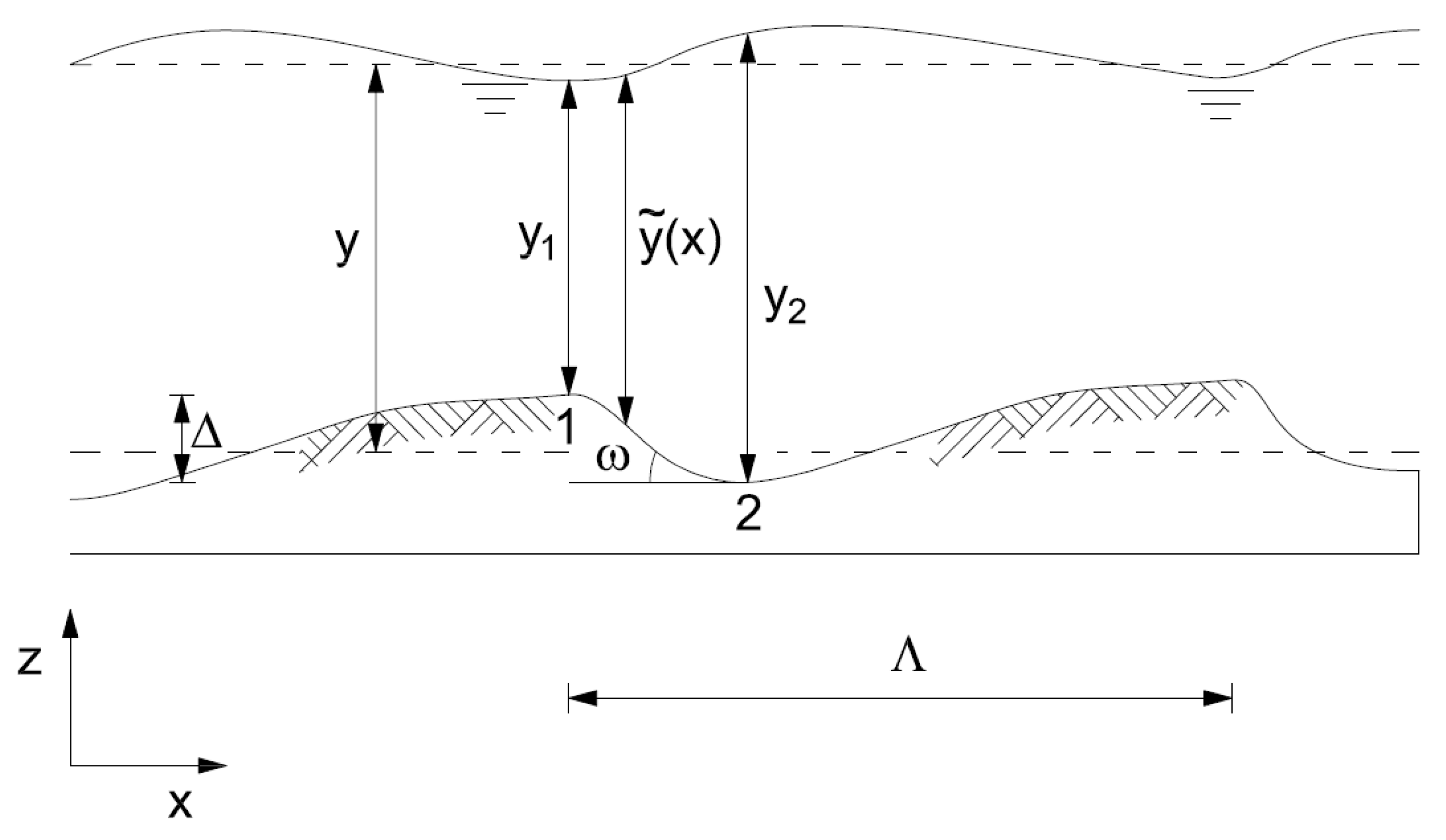
In a two-dimensional two-phase steady flow in presence of dunes (see Figure 1), the velocity distribution relates to the following characteristic parameters [15,28]:
where U is the mean flow velocity, y the mean flow depth, S the friction slope, ν and ρ the kinematic viscosity and the density of water, respectively, γs the specific weight of immersed sediment, ds the representative sediment diameter, Δ the dune height, Λ the dune length, and g the gravity acceleration. Therefore, it must hold a dimensionless general relationship of dependency on the following seven dimensionless parameters:
Assuming a constant value for the relative immersed weight of sediment in natural channels, and introducing the following dimensionless variables (i.e., relative submergence Z, Reynolds’ number Re and Froude number F):
the following relationship for the global friction slope is obtained:
So far, no theory analytically derives such a function, even for the simple reference case of steady, uniform 2D flow in a steady sediment transport condition. A possible approach consists in separating the global flow resistance into two individual contributions: surface roughness and macroroughness (i.e., bed form). Meyer-Peter and Muller [18] and Einstein [29] proposed a linear superposition assuming that the total bed shear stress (τ) could be separated into two contributions—plane bed stress (τ′) and additional shear stress—associated with the bed forms (τ″):
According to the assumed superposition of the effects, τ’ is equal to the shear stress acting on a sand-bed plane having the same grain-size distribution and the same hydrodynamic condition (i.e., velocity and flow depth). Later, Engelund [27] proposed that the total mean energy gradient per unit length of the stream (S) could be considered as a contribution of a friction loss (S′) due to the stress acting along the dune surface and of a cumulative loss due to a sudden flow expansion just downstream from the dune crest (S″):
and Equation (5) leads to:
Therefore, the total head loss (ΔH) over a stream reach of length L results from head loss due to the grain resistance (ΔH′) and head loss related to the dune (ΔH″):
3. Grain Contribution to Flow Resistance
The characteristics of the roughness elements located along the wetted perimeter affects the vertical profile of the downstream component and the resistance to flow. For fully developed turbulent flow over a rough sand-bed plane (Δ/y = Λ/y = 0), Re and F become irrelevant and the stream velocity profile can be expressed by a logarithmic law:
where u is the flow velocity at elevation z above the bed, k = 0.4 is the Von Karman’s constant, is the shear velocity related to the skin roughness and ks′ is the equivalent grain roughness. The vertically-averaged velocity U corresponds to the local velocity u at the relative depth z/y = e−1 = 0.368. By integration over the flow depth, it results:
where χ′ is the Chezy’s coefficient and C′ the dimensionless conveyance coefficient related to the skin roughness ks’. According to different Authors, ks′ is proportional to a characteristic sediment size ds, with subscript “s” being equal to 35, 50, 65, 84, 90 (i.e., the percentage of the finer particle size distribution by weight). Typically, ks′ ranges between 1.25 d35 and 5.10 d84 [1,2,3,4,5,6,7,8,9,16,30,31,32,33], whereas Millar [34] concluded that in gravel streams there is no significant difference between using d35, d50, d65, d84 or d90. In the present analysis, the mean grain size diameter d50 is assumed as a characteristic sediment size. Different values for ks were considered and the most appropriate value resulted ks = 2⋅d50.
In terms of slope friction, Equation (10) results:
which is consistent with Equation (4).
4. Sand Dune Contribution to Flow Resistance
In a two-dimensional two-phase steady flow in presence of dunes (see Figure 1), the momentum balance equation is applied to the reference control volume of a portion of 2D dune bed. The control volume is bounded between cross section 1 upstream, in correspondence to the crest of the dune, and cross section 2, downstream, in the trough zone where the streamlines are assumed to be parallel to the bed:
where P represents the pressure vector acting on the boundary of the fixed control between the two consecutive cross sections 1 and 2, G represents the mass force vector acting on the control volume and M represents the momentum flux vector through the boundary. The x-component of the previous equation gives:
being P1, P2, PL the pressure force acting on the upstream cross section, downstream cross section and on the lee side of the dune, respectively. TL is the shear stress on the lee side of the dune, M1 and M2 the momentum flux across the upstream and downstream cross sections 1 and 2, respectively, ω the angle between the lee dune side and the horizontal, and σ the average bed slope.
In a sand-bed river channel, the active longitudinal component of mass force G⋅sin(σ) can usually be disregarded with respect to the other forces. Since streamlines are parallel to the bed at cross sections 1 and 2, and the velocity in the flow separation zone may be considered null, hydrostatic pressure holds at both cross sections 1 and 2. The surface force component related to the shear stress (TL cos(ω)) is already included in the grain roughness component of the total resistance to flow. Introducing the momentum coefficient β (accounting for non-uniform velocity distribution over the cross section), the momentum balance equation per unit width of the channel becomes:
where yi is water depth at cross section (i = 1,2). The energy balance equation applied between cross sections 1 and 2 results:
where zi (i = 1,2) is the bed level and αi the Coriolis coefficient (i = 1,2) referred to cross sections 1 and 2. For the sake of simplicity from now on α1 = α2 = β1 = β2 = 1. The location of the stagnation point is not known a-priori and, taking into account for a mild slope of the toss face of the dune, it may be assumed z1−Δ = z2. Moreover, considering a reference dune bed pattern having a vertical dune lee side (i.e., ω = 90°), Equation (15) becomes:
and momentum balance Equation (14) leads to:
Disregarding the difference in water levels between cross sections 1 and 2, Equation (16) results:
It is convenient to refer to the mean water depth:
where is the local water depth (see Figure 1). For a dune bed-dominated river, the following approximation is considered [15]:
Introducing the water discharge per unit width of the channel:
and accounting for the mean water depth y (Equation (20)), results:
After algebraic simplification:
where the dune geometric correction function ΓΔ/y is:
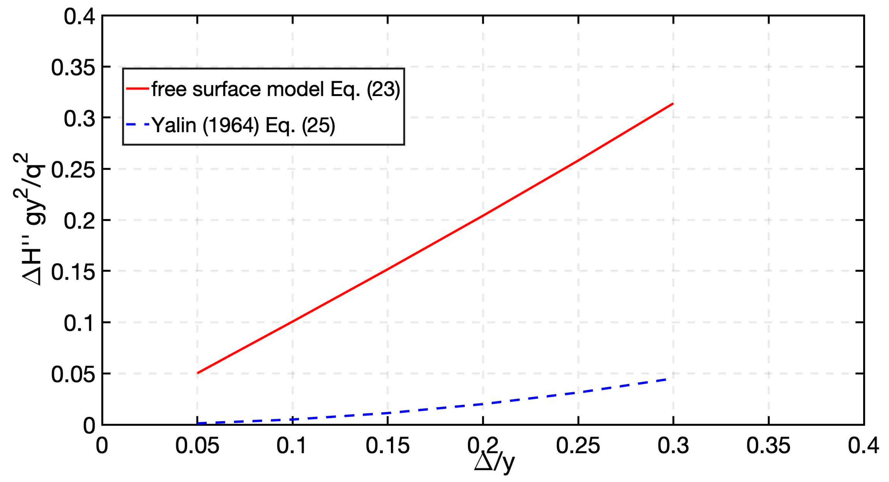
It is worth noting that Yalin [22] and Engelund [27], independently, applied a 1-D momentum conservation equation to the same dune bed reference pattern, but they assumed a constant pressure over the cross sections 1 and 2 (i.e., Borda–Carnot’s theorem for pressure pipe flow) rather than a hydrostatic pressure distribution, and they obtained:
where ΔHP″ indicates the bed form energy loss according to the pressure pipe flow approach. In this case:
A comparison of Equations (23) and (25) demonstrates the difference between the approach based on free surface flow instead of pipe flow, when the effects of sudden flow expansion in presence of dune is considered (Figure 2). Over the typical range of relative dune depth Δ/y = 0.1 − 0.3 the ratio between the two approaches, in terms of energy loss, varies from around 10 to 6. It supports the use of Equation (23) instead of Equation (25).
Using ΔH″ = S″⋅Λ, and after multiplying and dividing by the mean water depth (y), the energy slope related to the dune form drag results:
Empirical Coefficient for Bed Form Drag
Tokyay and Altan-Sakarya [35] tested the local energy losses at negative steps in subcritical open channel flows and demonstrated that energy losses are higher for inclined steps than for abrupt vertical steps. Van der Mark [36], following experimental results of flow over a single bed form with a vertical lee face concluded that an empirical coefficient should be applied to Equation (25) in order to take into account that flow velocity distribution is not uniform over the cross-section at the cross-sections 1 and 2. Engel [37] made experiments on the length of flow separation over artificial dunes in a flume, using fixed bed geometries. He showed that the separation length is independent of the Froude number, but it is dependent on the relative dune height Δ/y. Shen et al. [38] carried out laboratory experiments on rigid bed forms using both a rough and smooth surface. He showed that pressure drag coefficient relative to the bed form depends on the relative dune height, and on the dune slope steepness, whereas flow velocity and grain roughness does not influence it.
Therefore, the empirical correction coefficient κ, which is a function of the dune steepness δ = Δ/Λ, is introduced into Equation (27), to also take into account any differences between the theoretical and the actual flow field and bed form geometry, as a consequence of the assumptions so far introduced:
Using the breakdown of the energy slope S into its two components related to skin roughness S′ and bed form drag S″ (Equation (6)), Equation (28) gives the following expression for the empirical coefficient κ:
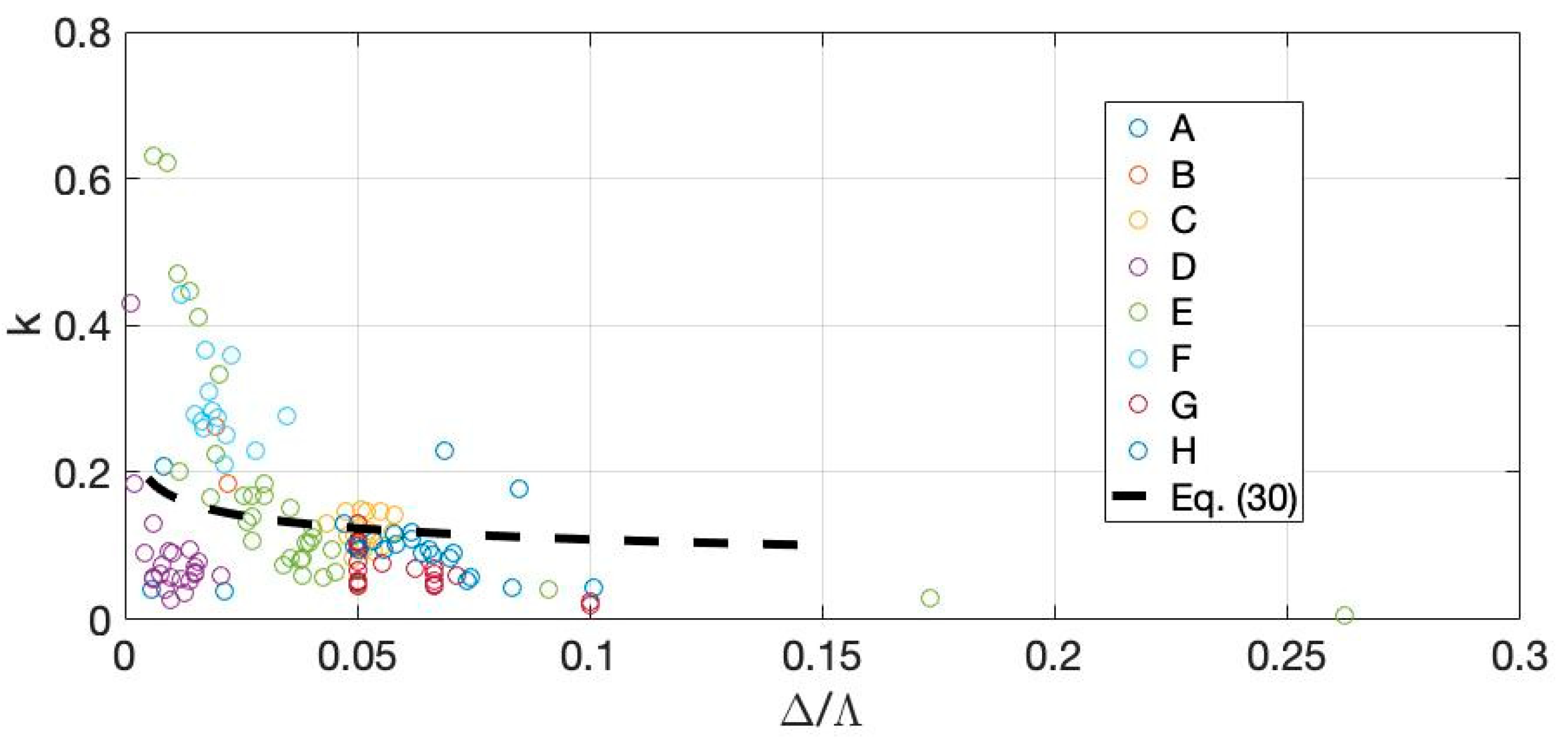
Once the bed dune geometry is known, considering the measured energy slope S, and after S′ is calculated by Equation (11) (assuming ks = 2·d50), it is possible to determine the empirical coefficient κ. A selection of 132 field data collected on 7 different sand-bed rivers with dune bed forms is considered (see Table 1). It refers to the Savio and Fiumi Uniti rivers [39], Calamus River [40], Missouri (data from Shen 1978, as reported by Brownlie [41]), Jamuna and Parana [42], Bergsche Maas (data from Adriaanse 1986, as reported by Julien [42]), and Meuse [42]. The database reports for each data set the number of measurements N, and the range of the following observed parameters: water discharge Q, mean depth y, mean flow velocity U, measured energy gradient S, Froude number F, mean grain size diameter d50, dune height Δ and dune length Λ. Despite the relative scatter of field data, Figure 3 shows how the drag coefficient decreases with increased dune steepness. Some outliers are present, corresponding to few data recorded on the Jamuna and Missouri rivers [42], characterized by very low values of dune steepness (i.e., Δ/Λ < 0.01), and filtered in the fitting procedures. The best fitting equation is:
with m = 0.053 and n = −0.2.
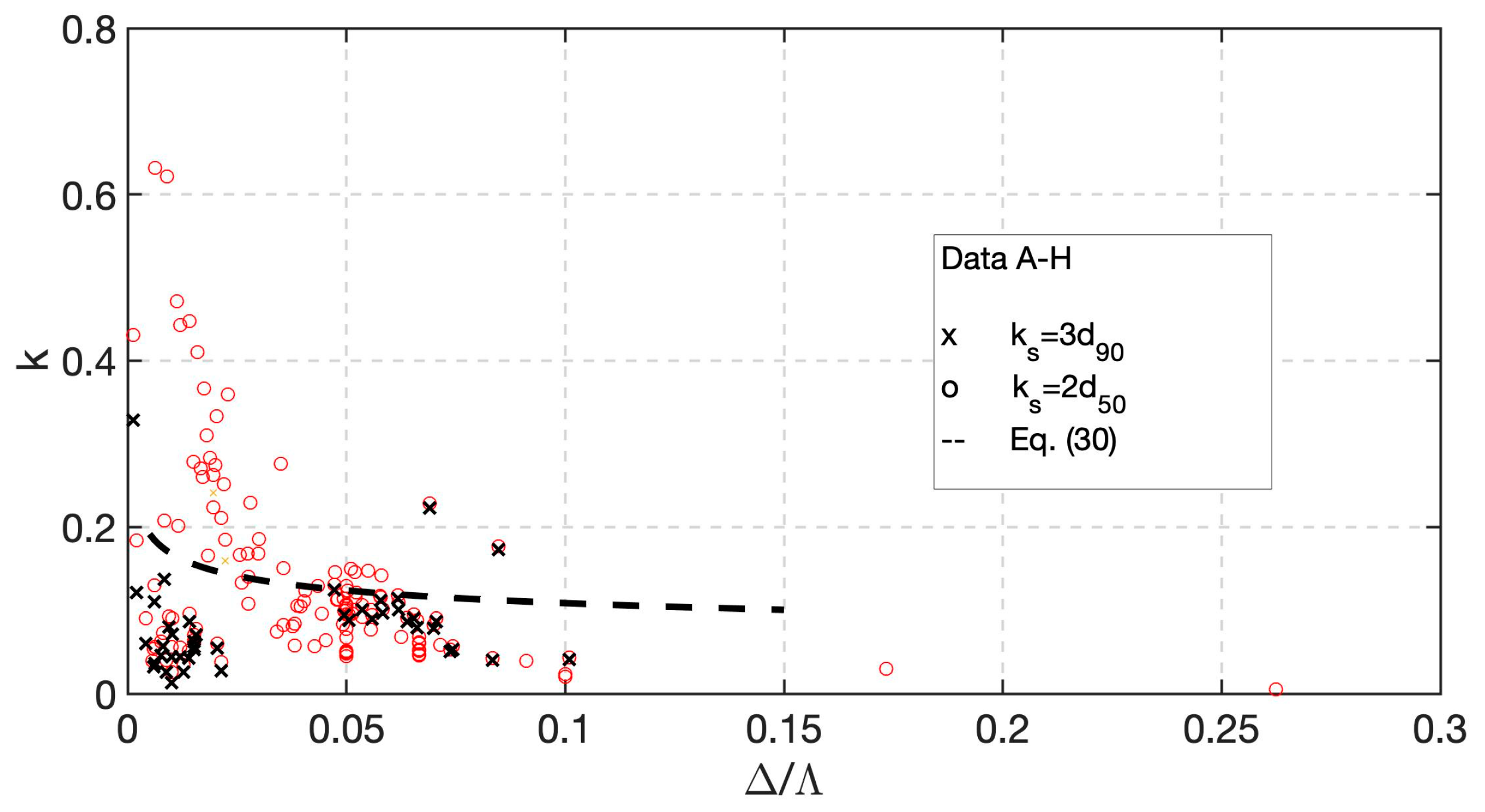
According to Equation (29), the estimated drag coefficient k depends on the skin energy slope (S′) which, in turn, depends on the equivalent roughness ks. Among the selected field data (river A–G, Table 1), Fiumi Uniti, Savio, Missouri and Meuse River reported information about sediment gradation or d90. Figure 4 shows a comparison between the drag coefficient κ obtained considering equivalent roughness ks = 2·d50 or ks = 3·d90.
The general trend remains confirmed, and it may be concluded that coefficient κ is almost independent of the equivalent skin roughness adopted to estimate the grain resistance contribution S′.
The dune steepness may be expressed by means of relative dune height and relative dune length, hence Equation (30) becomes:
The previous expression is particularly convenient, since according to several authors [10,15,24], the relative dune length may be considered as a constant. Thus, the drag coefficient remains as a function of the relative dune height and, after substituting Equation (31) in Equation (28), the bed form contribution to the energy slope is:
therefore, once the constant value for the relative dune length has been defined, the energy slope related to the dune drag results as a function only of the Froude number and of the relative dune height.
Introducing a constant value for the relative dune length Λ/y, the best fitting coefficients m and n may change from the previous values (m = 0.053 and n = −0.20) as will be discussed here in the model validation section.
5. Model Validation and Sensitivity Analysis to the Bed Form Geometry and Skin Roughness
In order to validate the proposed model a large selection of 491 field datasets is considered (Table 2), including those already used for the preliminary calibration of the empirical coefficient κ (Table 1). The Table 2 dataset refers to seventeen study reaches on five canals in Pakistan ACP-ACOP (data from Mahmood et al., 1979, as reported by Brownlie [41]), Niobrara River [43], Rio Grande (Culbertson et al. 1976, as reported by Brownlie [41]), 12 American canals in Nebraska, Colorado and Wyoming AMC (Simons 1957, as reported by Brownlie [41]), Middle Loup River (Hubble and Mateika 1959, as reported by Brownlie [41]), Atchafalaya (Toffaletti 1968 as reported by Brownlie [41]).
The model is validated comparing the observed and the estimated total energy slope (i.e., S = S’ + S″ Equation (6)), on the basis of the hydraulic parameters listed on Table 1 and Table 2.
In order to assess energy slope S, S′ is calculated by Equation (11) assuming ks′ = 2·d50, and S″ is calculated using Equations (32) and (24):
It results a parametric function of Froude number, dune geometry, and parameters m and n referred to the dune drag coefficient function (i.e., Equation (30)):
Therefore the energy slope related to the bed form drag (S″) in Equation (33) involves calculation of few parameters on the right-hand side of Equation (33). There are many empirical relationships in literature related to the bed form geometry. In the present work, the following have been considered (Van Rjin [10] and Karim [44], Equation (35) and Equation (36) respectively):
It is worth noting that Equation (36) gives relative dune height as a function of only hydraulic parameters, and equivalent skin roughness, because of introducing Equations (11) and (35) in Equation (36). Consequently, the best fitting parameters in Equation (32) result:
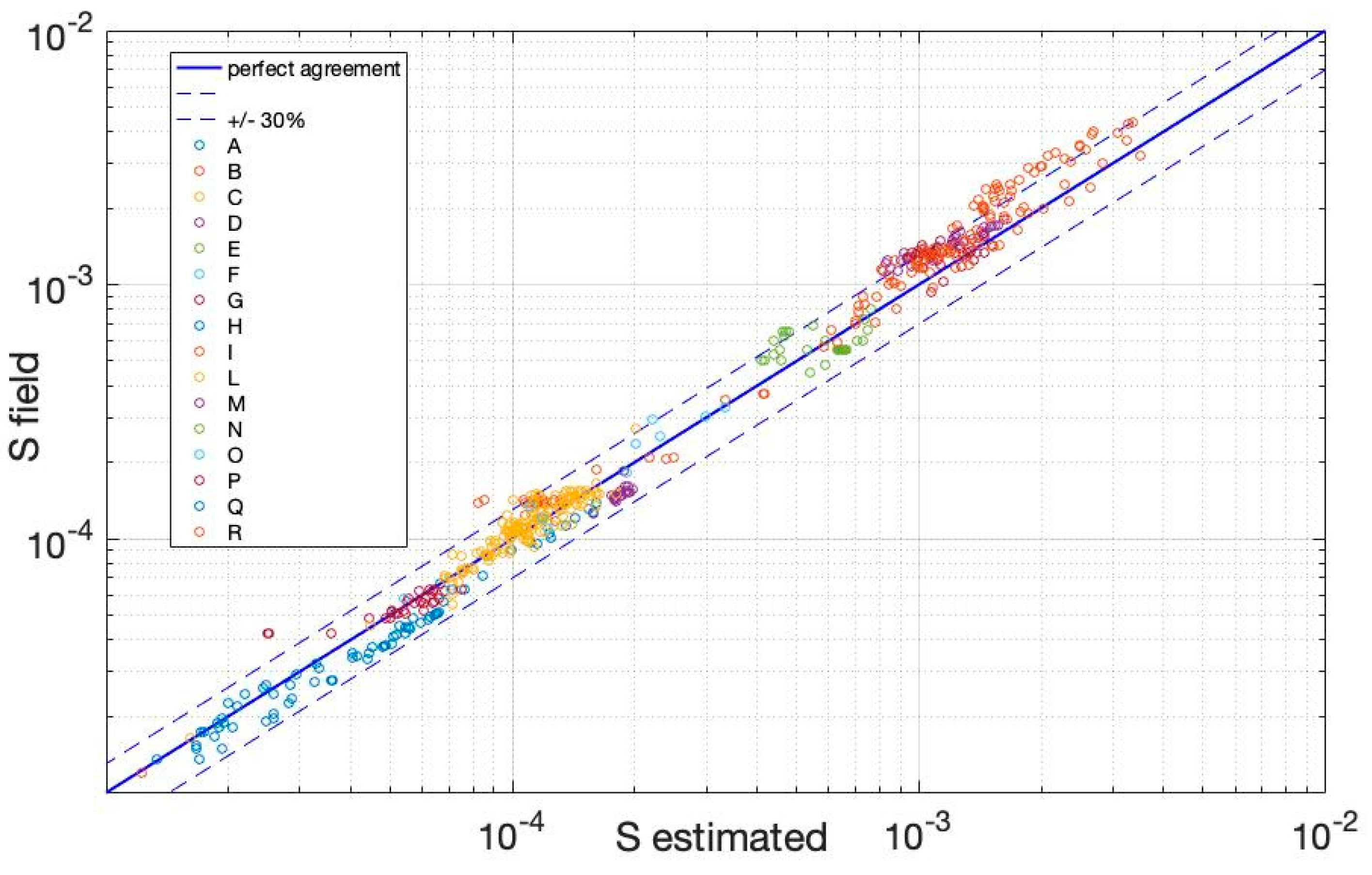
which are slightly different from those preliminary assessed (m = 0.053, n = 0.20). Figure 5 shows the comparison between calculated and measured energy slope.
m = 0.07 n = −0.19
Accounting for the observed water depth y and Froude number F (see column 5 and 8 in Table 1 and Table 2), the following equations are involved in energy slope calculation: S′ is calculated with Equation (11) assuming ks’ = 2·d50 (see column 9 in Table 1 and Table 2); S″ is calculated with Equation (33) along with parameters m and n from Equation (37), and eventually bed form steepness using Equations (35) and (36).
It is worth noting that in the range of observed mean flow velocity U, ranging 0.5–2.0 m/s, the skin roughness contribution gives a shear velocity u*’ = (g S′ y)0.5 in the range of about 0.02–0.06 m/s, and the dimensionless conveyance coefficient C = (g S y)0.5 respectively correspond to approximately 7–14 and 22–27.
Among the field data, 93.5% lies within the ±30% discrepancy band error and 68.2% of the measured energy slope lies within the ±20% band error. Considering the large uncertainties in field measurements, this can be considered as a good agreement.
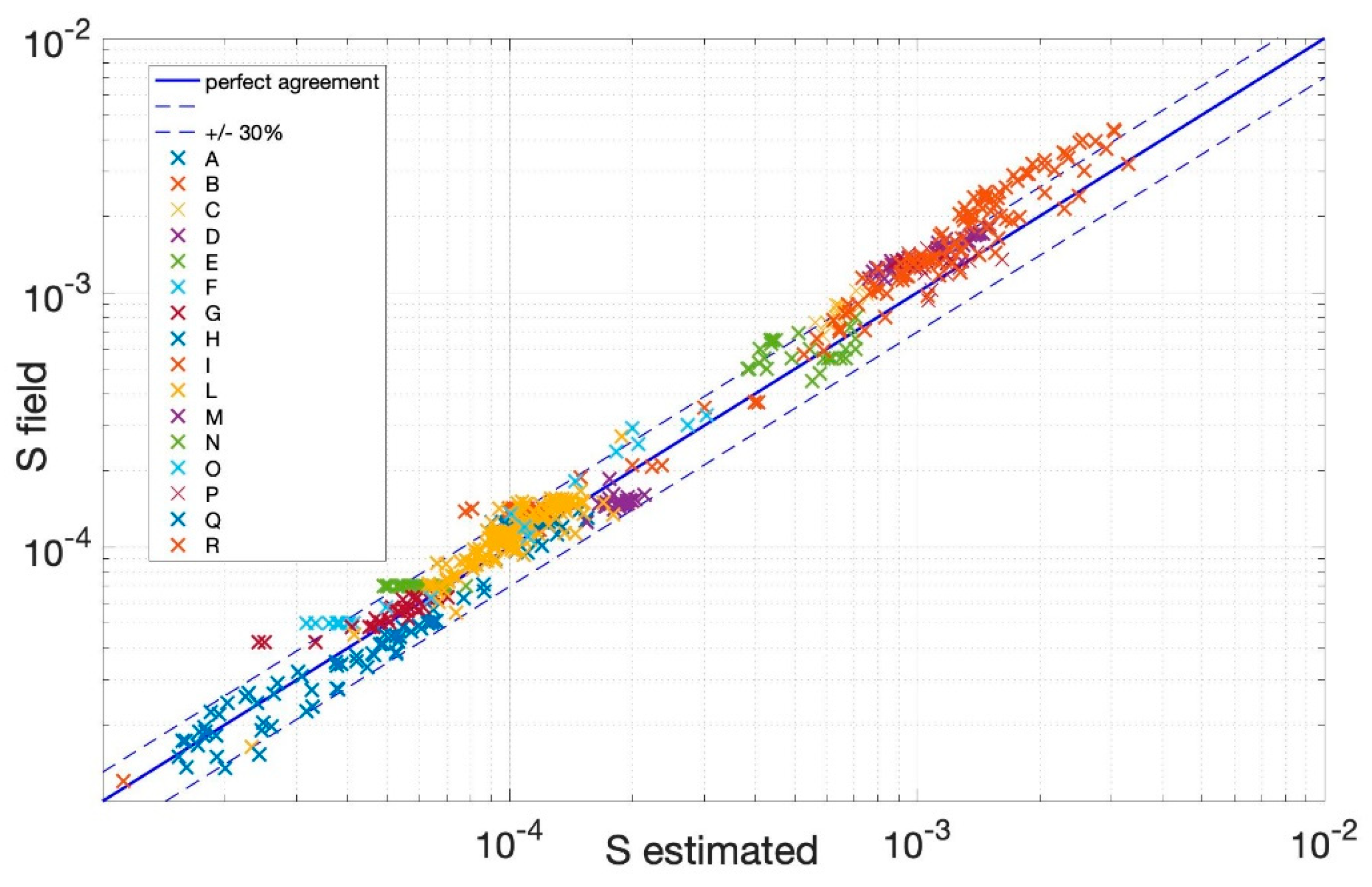
Skin roughness, as well as the adopted resistance formula, affects the grain flow resistance component and the related energy gradient calculation. Following the linear approach, the contribution due to the bed surface is equal to that of plane bed with identical hydraulic condition and sediment characteristic, without any bed form. The concepts of Karman–Prandtl logarithmic velocity distribution and Nikuradse equivalent grain roughness are considered (Equations (9) and (10)), where the latter is proportional to the characteristic grain size [45]. To test the sensitivity of the model, Nikuradse equivalent roughness ks′ = 1.0·d50 [46] and a different approach, reflecting Manning–Strickler Equation (38), are considered:
where n′ is Manning–Strickler coefficient related to the grain roughness. Hence:
and Equation (39) is used instead of Equation (11) to calculate the energy slope skin roughness contribution when Manning–Strickler formula is considered.
On the other hand, the assessment of bed form drag contribution involves dune geometry, in terms of dune steepness δ = Δ/Λ or, equivalently, the dimensionless dune height Δ/y and dimensionless dune length Λ/y (see Equation (33)). Different approaches proposed by Yalin [15,24], via empirical consideration based on field data, and reflecting theoretical consideration (Equations (40) and (41), respectively) were considered to explore the sensitivity of the proposed model to the dune geometry.
Table 3 reports the results of sensitivity analysis. Decreasing the value of Λ/y leads to a decreasing of the model accuracy. In fact, the field data included within the ±30% error band decrease from 93.5% to 91.3%, whereas the data included within the ±20% error band remains almost stable. By reducing the Nikuradse equivalent roughness (i.e., ks′ = 1 d50), field data included within the ±30% error band reduce from 93.5% to 90.7%, and the data included within the ±20% error band decrease from 68.4% to 65.5%. On the contrary, using the Manning–Strickler resistance formula (Equation (38)) only 88.2% of the predicted energy slope are within the ±30% band error and the data included within the ±20% band error are reduced to 65.5% (see Figure 6).
6. Conclusions
The focus of the present paper is the bed form contribution to the flow resistance in natural sand-bed rivers with dune bed forms, assuming a linear separation approach between skin roughness and dune bed form drag. To this aim, the momentum balance and the energy balance equations are applied to 2D flow in open channel, assuming hydrostatic pressure distribution over the cross sections bounding the control volume, which includes a reference bed form pattern. The related energy loss deviates from that derived by Borda–Carnot’s applied theorem. The resulting equation in terms of energy grade takes into account an empirical correction factor due to the actual flow field and bed form pattern. The empirical coefficient results as a power function of the dune steepness and is slightly dependent on the Nikuradse equivalent roughness of the grains. Thus, the dune contribution to the energy slope remains an explicit function of dune geometry, in terms of relative length and height, as well as Froude number. The model has been validated using 491 field measurements referred to sand rivers in presence of dunes, showing a good agreement. A sensitivity analysis on estimated energy slope was carried out in terms of dune geometry and the skin roughness adopted model. In particular, different relative dune length approaches were considered. Decreasing the relative dune length more than 30% of the reference value does not substantially degrade the model accuracy, whereas the model is relatively more sensitive to the Nikuradse equivalent roughness, and to the adopted resistance formula (e.g., Manning–Strickler formula).
Author Contributions
Conceptualization L.S.; methodology, L.S., S.C., P.C., P.B.; field investigation, S.C., P.C. and P.B.; data analysis L.S., P.B., P.C., S.C.; writing review and editing L.S., S.C., P.B., P.C.
Funding
This research received no external funding.
Conflicts of Interest
The authors declare no conflict of interest.
Abbreviations
| C′ | dimensionless conveyance Chezy coefficient related to the skin roughness |
| ds | representative sediment diameter |
| F | Froude number |
| g | gravity acceleration |
| G | mass force vector acting on the control volume of streamflow |
| k | Von Karman’s constant |
| ks’ | equivalent grain roughness |
| L | river reach length |
| m | fitting parameter of empirical correction function κ |
| M1, M2 | momentum flux in stream wise direction |
| M | momentum flux vector trough the surface of the control volume of the streamflow |
| n | fitting parameter of empirical correction function |
| n′ | Manning coefficient related to grain roughness |
| u | local flow velocity |
| shear velocity related to the skin roughness | |
| U | mean flow velocity |
| P1, P2,PL | pressure force acting on the upstream, downstream cross section, and on the lee side of the dune, with respect to the control volume of the streamflow |
| P | pressure vector acting on the boundary surface of the control volume of streamflow |
| q | water discharge per unit with of the channel |
| Re | Reynolds’ number |
| S | friction slope |
| S′ | friction slope due to the grain resistance |
| S″ | friction slope due to the dune drag |
| TL | shear stress on the lee side of the dune |
| y | mean flow depth |
| local water depth | |
| z | vertical elevation above the river bed |
| Z | relative submergence |
| αi | Coriolis coefficient |
| β | momentum coefficient |
| γs | specific weight of immersed sediment |
| ΓΔ/y and Γ PΔ/y | dune geometric correction function |
| δ | dune steepness |
| Δ | dune height |
| ΔH | total head loss |
| ΔH′ | head loss due to the grain resistance |
| ΔH″ | head loss due to the dune drag |
| ΔHP″ | head loss due to the dune drag according to pressure pipe flow approach |
| κ | empirical correction coefficient |
| Λ | dune length |
| ν | kinematic viscosity of water |
| ρ | density of water |
| σ | average river bedslope |
| τ | total bed shear stress |
| τ’ | grain shear stress contribution to the total bed shear stress |
| τ″ | bedform shear stress contribution to the total bed shear stress |
| ω | angle between the lee dune side and the horizontal |
References
- Cao, Z.; Carling, P.A. Mathematical modelling of alluvial rivers: Reality and myth. Part 1: General review. Proceedings of the Institution of Civil Engineers. Water Marit. Eng. 2002, 154, 207–219. [Google Scholar] [CrossRef]
- Wang, S.S.Y.; Wu, W. River sedimentation and morphology modeling—The state of the art and future development. In Proceedings of the 9th International Symposium on River Sedimentation, Yichang, China, 18–21 October 2004; pp. 71–94. [Google Scholar]
- Amoudry, L.O.; Souza, A.J. Deterministic coastal morphological and sediment transport modeling: A review and discussion. Rev. Geophys. 2011, 49. [Google Scholar] [CrossRef]
- Maldonado, S.; Borthwick, A.G.L. Quasi-two-layer morphodynamic model for bedload-dominated problems: Bed slope-induced morphological diffusion. R. Soc. Open Sci. 2018, 5, 172018. [Google Scholar] [CrossRef] [PubMed]
- Li, J.; Cao, Z.; Pender, G.; Liu, Q. A double layer-averaged model for dam-break flows over mobile bed. J. Hydraul. Res. 2013, 51, 518–534. [Google Scholar] [CrossRef] [Green Version]
- Iverson, R.M.; Ouyang, C. Entrainment of bed material by Earth-surface mass flows: Review and reformulation of depth-integrated theory. Rev. Geophys. 2015, 53, 27–58. [Google Scholar] [CrossRef]
- Abril, J.B.; Altinakar, M.S.; Wu, W. One-dimensional numerical modelling of river morphology processes with non-uniform sediment. In Proceedings of the River Flow 2012, San Jose, Costa Rica, 5–7 September 2012; pp. 529–535. [Google Scholar]
- Einstein, H.A.; Barbarossa, N.L. River channel roughness. Trans. Am. Soc. Civ. Eng. 1952, 117, 1121–1146. [Google Scholar]
- Engelund, F.; Hansen, E. A Monograph on Sediment Transport in Alluvial Streams; Teknisk Forlag: Copenhagen, Denmark, 1967; pp. 1–62. [Google Scholar]
- Van Rijn, L.C. Sediment Transport, Part III Bed Forms and Alluvial Roughness. J. Hydraul. Eng. ASCE 1984, 110, 1733–1755. [Google Scholar] [CrossRef]
- White, P.J.; Paris, E.; Bettess, R. The frictional characteristics of alluvial streams: A new approach. Proc. Inst. Civ. Eng. 1980, 69, 737–750. [Google Scholar] [CrossRef]
- Karim, M.F.; Kennedy, J.F. Menu of Coupled Velocity and Sediment Discharge Relations for Rivers. J. Hydraul. Eng. 1990, 116, 978–996. [Google Scholar] [CrossRef]
- Yang, S.; Tan, S. Flow resistance over mobile bed in an open channel flow. J. Hydraul. Eng. 2008, 134, 937–947. [Google Scholar] [CrossRef]
- Billi, P.; Salemi, E.; Preciso, E.; Ciavola, P.; Armaroli, C. Field measurement of bedload in a sand-bed river supplying a sediment starving beach. Z. Geomorphol. 2017, 61, 207–223. [Google Scholar] [CrossRef]
- Yalin, M.S. Mechanics of Sediment Transport, 2nd ed.; Pergamon Press: Oxford, UK, 1977. [Google Scholar]
- Van Rjin, L.C. Equivalent roughness of alluvial bed. J. Hydraul. Eng. Div. ASCE 1982, 118, 1215–1218. [Google Scholar]
- Yu, G.L.; Lim, S.Y. Modified Manning Formula for Flow in Alluvial Channels with SandBeds. J. Hydraul. Res. 2003, 41, 597–608. [Google Scholar] [CrossRef]
- Meyer-Peter, E.; Müller, R. Formulas for bed-load transport. In Proceedings of the 3rd Meeting of IAHR, Stockholm, Sweden, 7 June 1948; pp. 39–64. [Google Scholar]
- Azareh, S.; Afzalimehr, H.; Poorhosein, M.; Singh, V.P. Contribution of Form Friction to Total Friction Factor. Int. J. Hydraul. Eng. 2014, 2, 77–84. [Google Scholar]
- Yalin, M.S.; Karahan, E. Steepness of sedimentary dunes. J. Hydraul. Div. 1979, 105, 381–392. [Google Scholar]
- Julien, P.Y.; Klaassen, G. Sand dune geometry of large rivers during floods. J. Hydraul. Eng. 1995, 121, 657–663. [Google Scholar] [CrossRef]
- Yalin, M.S. On the average velocity of flow over a mobile bed. La Houille Blanche 1964, 1, 45–53. [Google Scholar] [CrossRef]
- Agarwal, V.C.; Ranga Raju, K.G.; Garde, R.J. Bed-form geometry in sand-bed flows; Discussion. J. Hydraul. Eng. 2001, 127, 433–434. [Google Scholar] [CrossRef]
- Yalin, M.S. Geometrical properties of sand waves. J. Hydraul. Div. 1964, 90, 105–119. [Google Scholar]
- Aberle, J.; Nikora, V.; Henning, M.; Ettmer, B.; Hentschel, B. Statistical characterization of bed roughness due to bed forms: A field study in the Elbe River at Aken, Germany. Water Resour. Res. 2010, 46. [Google Scholar] [CrossRef]
- Yang, S.; Tan, S.; Lim, S. Flow resistance and bed form geometry in a wide alluvial channel. Water Resour. Res. 2005, 41. [Google Scholar] [CrossRef] [Green Version]
- Engelund, F. Hydraulic resistance of alluvial streams. J. Hydraul. Div. 1966, 922, 315–326. [Google Scholar]
- Ferreira Da Silva, A.M.; Yalin, M.S. Fluvial Processes, 2nd ed.; IAHR Monograph; Taylor & Francis Group: London, UK, 2017. [Google Scholar]
- Einstein, H.A. The Bed Load Function for Sediment Transportation in Open Channel Flows; Technical Bulletin 1026; U.S. Dept of Agriculture Soil Conservation Service: Washington, DC, USA, 1950.
- Ackers, P.; White, W. Sediment Transport: New Approach and Analysis. J. Hydraul. Div. 1973, 99, 2041–2060. [Google Scholar]
- Hey, R.D. Flow Resistance in Gravel-Bed Rivers. J. Hydraul. Div. 1979, 105, 365–379. [Google Scholar]
- Kamphuis, J.W. Determination of sand roughness for fixed beds. J. Hydraul. Res. 1974, 12, 193–203. [Google Scholar] [CrossRef]
- Whiting, P.J.; Dietrich, W.E. Boundary shear stress and roughness over mobile bed. J. Hydraul. Eng. 1990, 116, 1495–1511. [Google Scholar] [CrossRef]
- Millar, R.G. Grain and form resistance in gravel-bed rivers Résistances de grain et de forme dans les rivières à graviers. J. Hydraul. Res. 1999, 37, 303–312. [Google Scholar] [CrossRef]
- Tokyay, N.D.; Altan-Sakarya, A.B. Local energy losses at positive and negative steps in subcritical open channel flows. Water SA 2011, 37, 237–244. [Google Scholar] [CrossRef]
- van der Mark, C.F. A Semi-Analytical Model for Form Drag of River Bedforms. Ph.D. Thesis, University of Twente, Twente, The Nederlands, 1978. [Google Scholar]
- Engel, P. Length of flow separation over dunes. J. Hydraul. Div. 1981, 107, 1133–1143. [Google Scholar]
- Shen, H.W.; Fehlman, H.M.; Mendoza, C. Bed form resistances in open channel flows. J. Hydraul. Eng. 1990, 116, 799–815. [Google Scholar] [CrossRef]
- Cilli, S.; Ciavola, P.; Billi, P.; Schippa, L. Moving dunes constrain flow hydraulics in mobile sand-bed streams: The Fiumi Uniti and Savio River cases (Italy). Geomorphology 2019. submitted for publication. [Google Scholar]
- Gabel, S.L. Geometry and kinematics of dunes during steady and unsteady flows in the Calamus River, Nebraska, USA. Sedimentology 1993, 40, 237–269. [Google Scholar] [CrossRef]
- Brownlie, W.R. Compilation of Alluvial Channel Data: Laboratory and Field; Report No. KH-R-43B; California Institute of Technology, WM Keck Laboratory of Hydraulics and Water Resources Division of Engineering and Applied Science: Pasadena, CA, USA, 1981; pp. 1–209.
- Julien, P. Study of Bedform Geometry in Large Rivers; Report Q 1386 Delft Hydraulics; Delft Hydraulics: Delft, The Netherlands, 1992; pp. 1–79. [Google Scholar]
- Colby, B.R.; Hembxee, C.H. Computation of Total Sediment Discharge, Niobrara River Near Cody, Nebraska; Geological survey water-supply paper 1357; U.S. Government Printing Office: Washington, DC, USA, 1955; pp. 1–187. [CrossRef]
- Karim, F. Bed form geometry in sand dunes. J. Hydraul. Eng. 1999, 152, 1253–1261. [Google Scholar] [CrossRef]
- Yen, B.C. Open Channel Flow Resistance. J. Hydraul. Eng. 2002, 128, 20–39. [Google Scholar] [CrossRef]
- Keulegan, G.H. Laws of turbulent flow in open channels. J. Res. Nalt. Bur. Stand. 1938, 21, 707–741. [Google Scholar] [CrossRef]
Figure 1.
Schematic representation of 2-D flow in presence of dune.

Figure 2.
Difference between free surface flow approach, and pressure pipe flow approach.


Figure 4.
Empirical drag coefficient κ as a function of dune steepness δ = Δ/Λ. Comparison between results obtained by using different equivalent roughness ks (Data A–G see Table 1).
Figure 4.
Empirical drag coefficient κ as a function of dune steepness δ = Δ/Λ. Comparison between results obtained by using different equivalent roughness ks (Data A–G see Table 1).

Figure 5.
Comparison of estimated and observed total energy slope (the dashed lines represent the ±30% error band).
Figure 5.
Comparison of estimated and observed total energy slope (the dashed lines represent the ±30% error band).

Figure 6.
Comparison of estimated and observed total energy slope (the dashed lines represent the ±30% error band). Note: the total energy slope S is calculated accounting for the grain component S′ obtained by Manning–Strickler Equation (39).
Figure 6.
Comparison of estimated and observed total energy slope (the dashed lines represent the ±30% error band). Note: the total energy slope S is calculated accounting for the grain component S′ obtained by Manning–Strickler Equation (39).


Table 1.
Summary of field data used to determine empirical coefficient κ (Equation (29)). Each column reports maximum and minimum value.
Table 1.
Summary of field data used to determine empirical coefficient κ (Equation (29)). Each column reports maximum and minimum value.
| Code | River | N | Q (m3/s) | Y (m) | U (m/s) | S (m/km) | F (-) | d50 (mm) | d90 (mm) | Δ (m) | Λ (m) |
|---|---|---|---|---|---|---|---|---|---|---|---|
| A | Fiumi Uniti | 22 | 358.40–21.17 | 4.72–1.31 | 1.66–0.20 | 0.139–0.002 | 0.24–0.04 | 0.655–0.390 | 2.100–0.630 | 0.28–0.10 | 17.53–13.1 |
| B | Savio | 9 | 132.06–7.04 | 3.58–1.77 | 1.50–0.21 | 0.354–0.012 | 0.28–0.05 | 0.548–0.412 | 1.702–0.694 | 0.16–0.12 | 7.16–6.14 |
| C | Calamus | 18 | 1.73–0.82 | 0.61–0.34 | 0.77–0.61 | 1.100–0.680 | 0.34–0.29 | 0.410–0.310 | - | 0.20–0.10 | 4.05–2.02 |
| D | Missouri | 25 | 1817.20–179.20 | 4.99–2.77 | 1.76–1.28 | 0.185–0.125 | 0.32–0.22 | 0.266–0.190 | 0.311–0.217 | 2.07–0.58 | 735.18–57.91 |
| E | Jamuna | 33 | 10000–5000 | 19.50–8.20 | 1.50–1.30 | 0.070 | 0.17–0.09 | 0.200 | - | 5.10–0.80 | 251.00–8.00 |
| F | Parana | 13 | 25000 | 26.00–22.00 | 1.50–1.00 | 0.050 | 0.10–0.07 | 0.370 | - | 7.50–3.00 | 450.00–100.00 |
| G | Zaire | 29 | 28490–284 | 17.60–6.80 | 1.69–0.32 | 0.345–0.042 | 0.16–0.03 | 0.545–0.430 | 1.900–0.430 | 1.90–1.20 | 450.00–90.00 |
| H | Bergsche Maas | 20 | 2160 | 10.50–5.80 | 1.70–1.30 | 0.125 | 0.20–0.13 | 0.520–0.210 | - | 2.50–0.40 | 50.00–6.00 |
Table 2.
Summary of field data used to validate the model.
| Code | River | N | Q (m3/s) | Y (m) | U (m/s) | S (m/km) | F (-) | d50 (mm) | d90 (mm) | Δ (m) | Λ (m) |
|---|---|---|---|---|---|---|---|---|---|---|---|
| I | Meuse | 44 | 1743.0–1731.0 | 9.52–8.22 | 1.57–0.87 | 0.141–0.138 | 0.17–0.09 | 0.650–0.500 | 2.500–1.030 | 0.85–0.58 | 13.42–7.03 |
| L | ACP–ACOP | 151 | 528.68–27.50 | 4.30–0.76 | 1.29–0.35 | 0.271–0.016 | 0.23–0.12 | 0.364–0.083 | 0.466–0.105 | - | - |
| M | Niobrara | 40 | 16.06–5.86 | 0.59–0.40 | 1.27–0.65 | 1.799–1.136 | 0.54–0.30 | 0.359–0.212 | 0.849–0.326 | - | - |
| N | Rio Grande | 33 | 42.19–1.67 | 1.51–0.39 | 1–69–0.10 | 0.800–0.450 | 0.49–0.04 | 0.280–0.160 | 0.417–0.198 | - | - |
| O | AMC | 11 | 29.42–1.22 | 2.53–0.80 | 0.79–0.42 | 0.3300.058 | 0.25–0.10 | 7.000–0.096 | 1.440–0.331 | - | - |
| P | MID | 38 | 13.62–9.03 | 0.41–0.25 | 1.12–0.59 | 1.572–0.929 | 0.72–0.32 | 0.436–0.215 | 1.264–0.346 | - | - |
| Q | ATC | 55 | 14186.31–1449.78 | 14.75–6.92 | 2.03–0.64 | 0.051–0.014 | 0.17–0.06 | 0.303–0.085 | 0.708–0.169 | - | - |
Table 3.
Sensitivity analysis of the bed surface roughness and the dune geometry predictor.
| Dataset | Λ/y | S′ | Validated Data within Error Band | |
|---|---|---|---|---|
| 30% | 20% | |||
| model | 7.30 | Equation (11) ks’ = 2.0·d50 | 93.5% | 68.4% |
| test | 6.28 | 93.1% | 69.4% | |
| test | 5.00 | 91.3% | 68.6% | |
| test | 7.30 | Equation (11) ks’ = 1.0·d50 | 90.7% | 62.5% |
| test | Equation (38) | 88.2% | 63.9% | |
© 2019 by the authors. Licensee MDPI, Basel, Switzerland. This article is an open access article distributed under the terms and conditions of the Creative Commons Attribution (CC BY) license (http://creativecommons.org/licenses/by/4.0/).
Share and Cite
MDPI and ACS Style
Schippa, L.; Cilli, S.; Ciavola, P.; Billi, P. Dune Contribution to Flow Resistance in Alluvial Rivers. Water 2019, 11, 2094. https://doi.org/10.3390/w11102094
AMA Style
Schippa L, Cilli S, Ciavola P, Billi P. Dune Contribution to Flow Resistance in Alluvial Rivers. Water. 2019; 11(10):2094. https://doi.org/10.3390/w11102094
Chicago/Turabian StyleSchippa, Leonardo, Silvia Cilli, Paolo Ciavola, and Paolo Billi. 2019. "Dune Contribution to Flow Resistance in Alluvial Rivers" Water 11, no. 10: 2094. https://doi.org/10.3390/w11102094
Note that from the first issue of 2016, this journal uses article numbers instead of page numbers. See further details here.