Quantifying the Uncertainty Related to Climate Change in the Assessment of Urban Flooding—A Case Study


Facoltà di Ingegneria ed Architettura, Università degli Studi di Enna Kore, 94100 Enna, Italy
*
Author to whom correspondence should be addressed.
Water 2019, 11(10), 2072; https://doi.org/10.3390/w11102072
Submission received: 10 August 2019
/
Revised: 24 September 2019
/
Accepted: 1 October 2019
/
Published: 4 October 2019
(This article belongs to the Special Issue Urban Rainfall Analysis and Flood Management)
Abstract
:Recent studies have pointed out that climate change is likely to have important implications on the extent and frequency of flooding events. Indeed, the intensification of the water cycle occurring in different areas of the world can dramatically affect the incidence of extreme events and, consequently, the flow in rivers or artificial channels, increasing the probability of disastrous floods. In this context, the criteria for the assessment of flood risk need to be improved to take into account the variability of rainfall due to climate change. In this study, a Bayesian procedure was used to update the parameters of the depth–duration–frequency (DDF) curves and quantify the uncertainty related to their assessment in some climate change scenarios. The critical storm obtained from these updated DDF curves was used as input for the FLO-2D hydraulic model, in order to investigate the effects of climate change on flood risk. The area of study was an urban catchment in Piazza Armerina, a small town located in Southern Italy. Results showed that rainfall variations remarkably affect not only the magnitude of flood events, but also the flood susceptibility of the study area.
1. Introduction
The design criteria of an urban drainage system are based on the knowledge and prediction of rainfall extremes. In recent decades, extreme rainfall events have become more intense and frequent worldwide, due to the increase of the average global air temperature and the concentration of the atmospheric water vapor [1,2,3]. The increased occurrence of extreme rainfall events is expected to alter the magnitude and frequency of peak flows over the service life of urban drainage systems [4]. Repeated floods have already affected different urban areas in Europe, causing serious and costly damages [5,6].
Several studies have investigated the impact of climate change on urban flooding. In most cases, these studies were based on projected changes in extreme rainfall to account for the effect of climate change on urban flooding and highlighted that, in regions where climate change occurs, systemic adaptation measures should be adopted to reduce impacts on the performance of the drainage systems [7]. In Australia, Schreider et al. [8] estimated the changes in the potential damage of flood events caused by climate change in three catchments near Sidney and Canberra. In Canada, Denault et al. [9] used the SWMM model to analyze the potential impacts of changes in short duration rainfall intensity on urban drainage systems in the Mission/Wagg Creek watershed (Canada). In the USA, Markus et al. [10] developed a methodology for diagnostic analysis of future climate scenarios applied to urban flooding in Chicago. Huong and Pathirana [11] used a 1-D/2-D coupled urban drainage/flooding model (SWMM-Brezo) model to estimate the changes in flood hazard in the city of Can Tho (Vietnam) in some future climate scenarios. Zhou et al. [12] investigated the performance of a drainage system in Hohhot (northern China) in different climate scenarios, exploring the role of mitigation and adaptation measures in reducing urban flood. In Brazil, da Silva et al. [13] used updated intensity–duration–frequency (IDF) curves to analyze the effects of climate change on an urban drainage system. More recently, Andimuthu et al. [14] generated IDF curves for a 2-, 5-, 10-, 50-, and 100-year return period under the current and future climate for an Indian coastal city. An integrated hydraulic and hydrological modeling was used to assess the flood-carrying capacity of the drainage system in these scenarios.
As regards European countries, studies were carried out in Sweden, Denmark, the UK, Belgium, and Italy. In Sweden, Olsson et al. [15] analyzed the impact of climate change on an urban drainage system applying the sewer simulation software MOUSE for the city of Kalmar. In Denmark, Kaspersen et al. [16] combined remote sensing and the MIKE 21 model to quantify the implications of change in imperviousness and climate on flood risk in Odense. Ashley et al. [17] analyzed the current and future pressure on planning, design, operation, and maintenance of urban drainage infrastructures in the UK. More recently, Adbellatif et al. [18] carried out an assessment of climate change impact of flood risk in an urban drainage catchment located in Northwestern England, using an artificial neural network (ANN) downscaling technique to obtain local scale future rainfall from three coarse scale general circulation models (GCM). In Belgium, Willems et al. [19] simulated the effects of climate change on sewer overflow frequencies using a continuous simulation reservoir-based model. Archetti et al. [20] studied the behavior of the sewer network in Rimini (Italy), proposing a simplified method to evaluate the urban flooding severity as a function of climate variables.
The analysis of previous research highlighted that the identification and the quantification of extreme rainfall variations and trends has a considerable role in the definition of potential future climate scenarios [21]. Specifically, methodologies and techniques need to be developed to integrate the trend magnitude in the calculation of the parameters of the depth–duration–frequency (DDF) curves, which are commonly used for the assessment of the design storm for urban drainage systems [22,23].
The main objective of this study was the analysis and quantification of the potential implications of climate change on urban drainage systems and, consequently, on urban flooding. In this study, the Bayesian procedure proposed by Liuzzo et al. [23] was applied to define the DDF curves for different climate change scenarios in Piazza Armerina, a small town located in Southern Italy. Once the design storms were estimated using the updated DDF curves, these results were used as input for the two-dimensional hydraulic model FLO-2D hydraulic model [24]. The simulations performed by means of FLO-2D were used to quantify the impacts of the detected rainfall change on the flood risk in the area of study. Results allowed evaluating the applicability and reliability of the abovementioned Bayesian procedure in the investigation of climate change effects on the performance of urban drainage systems.
2. Materials and Methods
2.1. Case Study and Dataset
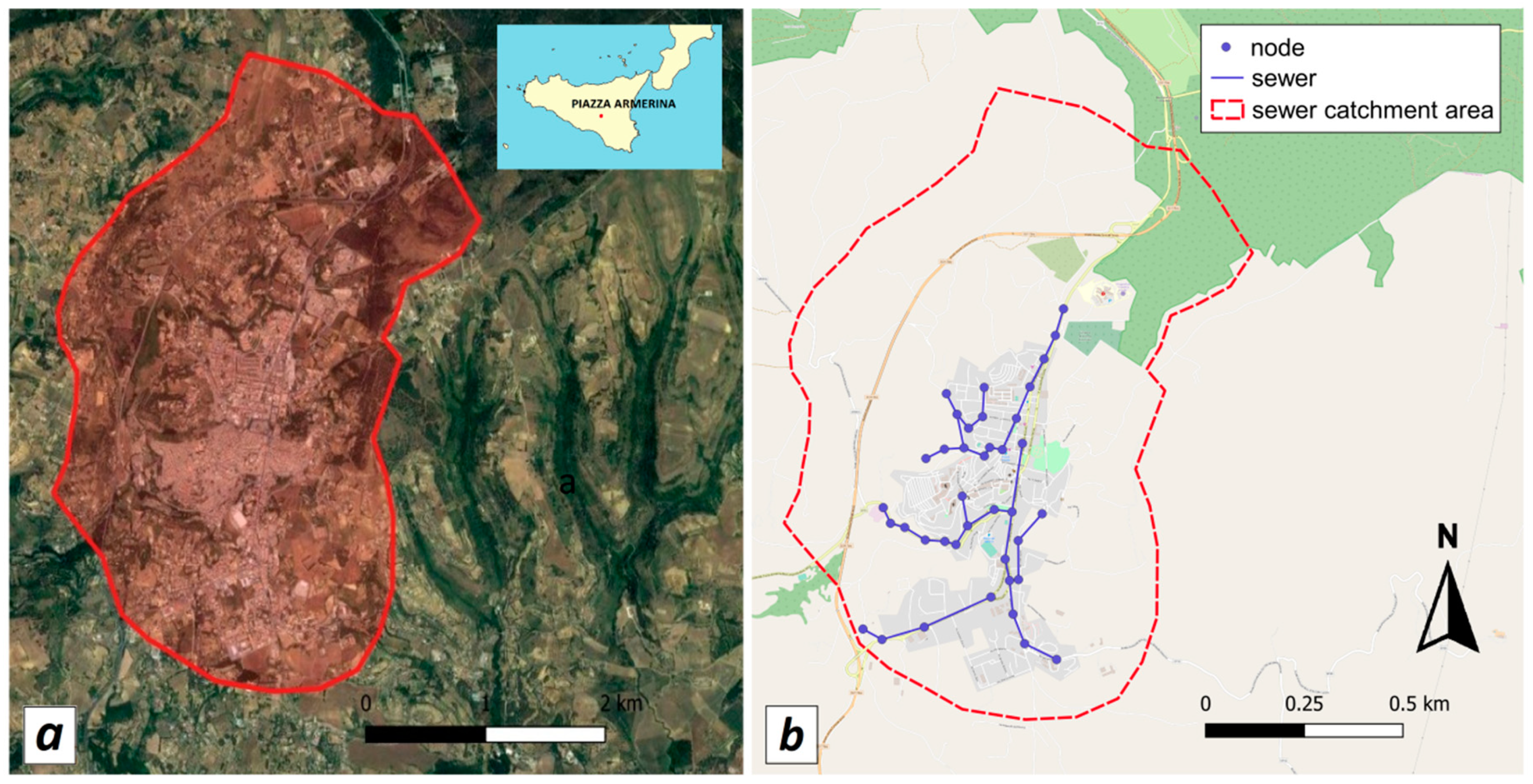
In this study, the urban drainage system of Piazza Armerina was analyzed. Piazza Armerina is a small town with a population of approximately 21,700 inhabitants, located in the central–eastern part of Sicily (Southern Italy). In this area, the climate is characterized by mild winters and hot and generally dry summers. Figure 1a shows the location of Piazza Armerina. The available historical annual maxima rainfall series of durations 1, 3, 6, 12, and 24 h recorded in Piazza Armerina during 1956–2008 were provided by Osservatorio delle Acque della Regione Sicilia.
The Piazza Armerina watershed is moderately urbanized, with an area equal to 11 km2, consisting of about 45.5% of impervious areas and 54.5% of pervious areas. The impervious area is mainly concentrated in the central part of the catchment being characterized by the urban city centre. The 92% of the constructed area is concentrated in the city center (4.7 km2); the remaining 8% is due to rural buildings and infrastructures around the center. The urban catchment is drained by a combined sewer system designed in HDPE (high-density polyethylene), considering a return period of 10 years. The design is rather new, and the network was completely redesigned in 2002 and rebuilt between 2004 and 2005. The total pipe length is approximately 74 km (considering only the main and secondary pipes, so neglecting service connections and pipes with a diameter smaller than 200 mm). As the present paper is focused on flooding only, the main pipes were simulated having diameters higher than 500 mm, being 23% of the total length (around 17 km). The concentration time of the considered urban catchment is about 2.1 hours. The DDF curve used for design purposes was evaluated by means of univariate statistical analysis of the annual maxima series recorded at the Piazza Armerina rain gauge during the 1956–2008 period.
In this study, to simulate the hydraulic behavior of the urban drainage system both for the current climate conditions and the climate change scenarios, the FLO-2D model was used. Figure 1b shows the network schematic employed in the FLO-2D to simulate the hydraulic behavior of the analyzed drainage system in the abovementioned scenarios.
2.2. Estimation of DDF Curve Parameters in Climate Change Scenarios
The DDF curves are widely used in hydraulic and hydrological engineering applications to assess the design storm for a specified return period and event duration. Thus, reliable estimations of the DDF curves parameters are necessary for the optimal design of hydraulic infrastructures. The DDF relationship for the return period T often takes the form of a power law relationship:
where h(d)T is the rainfall depth at the specified return period T, duration d, and aT and nT are parameters. According to previous studies, the annual maxima rainfall trends occurring in Sicily are because of variations of the aT parameter [25,26]. By means of the Bayesian procedure described in detail by Liuzzo et al. [23] the aT parameter of Equation (1) was estimated for some future scenarios.
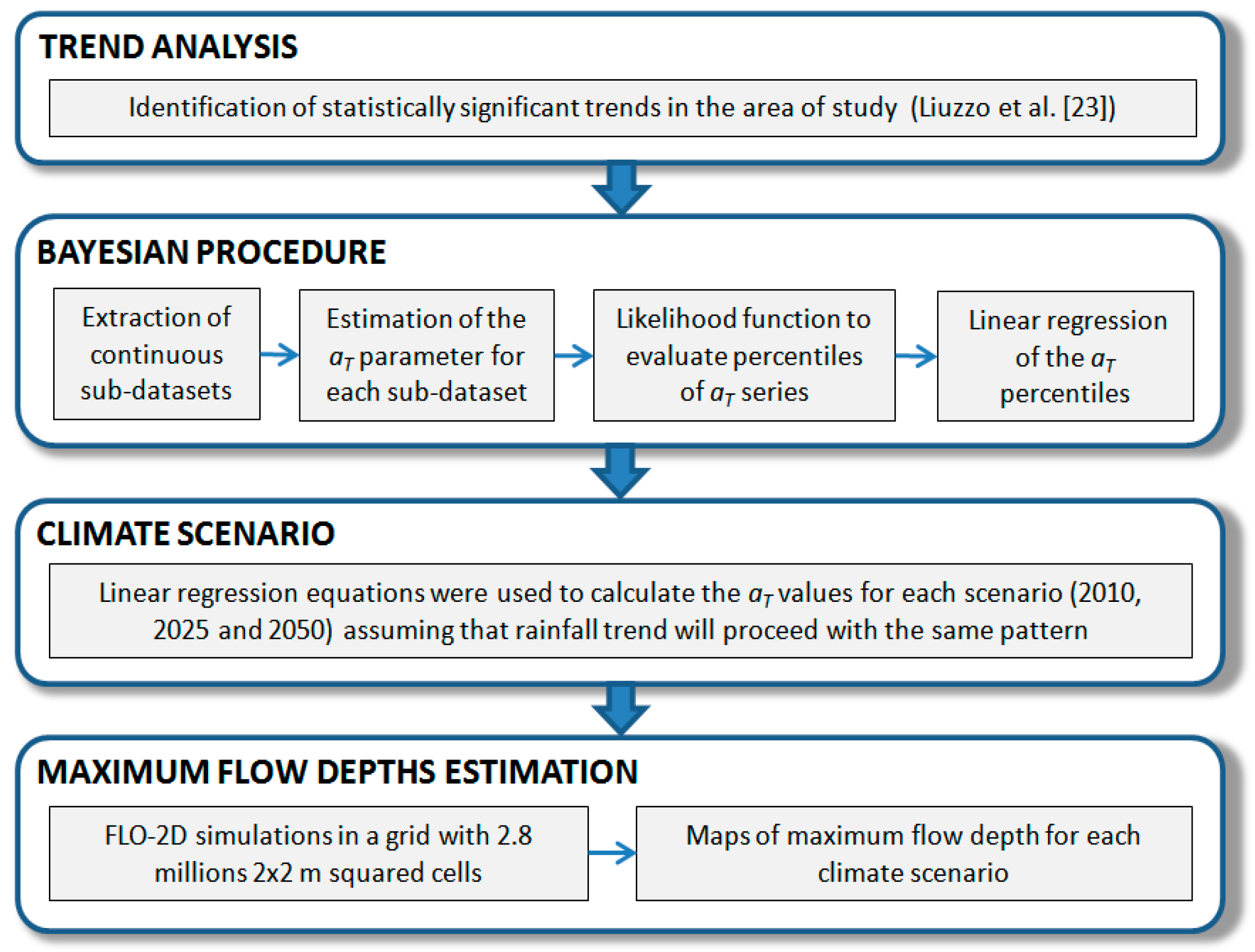
The Bayesian procedure allowed assessing the uncertainty linked to the aT parameter of the DDF curve in the presence of an annual maxima rainfall trend. Specifically, the procedure was applied to incorporate, in the DDF curve parameters, the effect of the statistically significant trends of annual maximum rainfall of 1-hour duration. The methodology can be briefly summarized as follows:
- From the original dataset, several continuous sub-datasets with different ending years and lengths were extracted. Specifically, starting from a minimum of 15 years, the length of each sub-dataset was increased by one, up to a maximum of 35 years. This choice was based on the evidence that an intensification of the hydrological cycle occurred in the last 30–35 years [27]. Moreover, this assumption is furtherly supported by the evidence of a statistically significant increase of the average annual rainfall during the last 30 years in Sicily [28];
- The aT parameter was estimated for each of the above-mentioned sub-datasets;
- The likelihood function was used to evaluate the 95th, 50th, and 5th percentiles of each aT series.
To define a mathematical law of the aT variability in time, a linear regression of the aT percentiles was performed considering the last 30 years of the series.
The 95th and 5th percentile regression laws represent, respectively, the upper and lower uncertainty bands related to the estimation of the aT parameter, and the width of these bands provides a quantification of the uncertainty in the aT appraisal.
To investigate the implications of climate change on urban flooding, some climate scenarios were generated. Among the different methodologies in literature for climate scenario generation, the temporal analogue approach [29] was chosen. According to this consolidated and frequently used methodology, in the generation of climate projections, the linear variation of precipitation over the past years, detected by trend analysis, was used, assuming that future climate will be characterized by the same pattern. Therefore, the previously defined regressions were used to extrapolate the aT parameter values for the short-term projections to 2025 and 2050. Figure 2 shows the flow chart of the entire procedure applied in this study.
Results were compared to the current conditions scenario, represented by the estimation of aT in 2010. The aT parameters were evaluated using the generalized extreme value (GEV) distribution for four return periods T: 2, 5, 10, and 20 years.
It has to be remarked that the addition of recent data to the original dataset requires reapplying the procedure including the new data. Indeed, the addition of new data could affect the results of the linear regression changing the direction and the magnitude of the trend.
2.3. The Hydraulic Model: FLO-2D
In the urban catchment, flood routing was carried out using the two-dimensional hydraulic model FLO-2D (http://www.flo-2d.com/). The governing equations include the continuity equation and the two-dimensional equations of motion (dynamic wave momentum equation):
where h is the flow depth (m); u and v are the depth-averaged velocities in the x-axis and y-axis directions, respectively; i is the excess rainfall intensity (mm/h); Sfx and Sfy are the friction slope components according to Manning’s equation of the x-axis and y-axis direction, respectively; Sbx and Sby are the bed slope of the x-axis and the y-axis directions, respectively; and g is the gravity acceleration (m/s2).
The model governing equations were solved on a grid of square elements in the eight flow directions using a finite difference method. The initial velocity was computed applying Manning’s equation in one direction. The algorithm calculates the discharge across each of the boundaries in the eight directions. Each grid element computation starts with the assessment of the linear flow depth at the boundary of the grid element. The estimated boundary flow is the average of the flow depths in the two grid elements sharing discharge in one of the eight directions. Other hydraulic parameters, such as flow resistance, flow area, etc., are averaged to calculate the flow velocity.
Once the hydraulic simulations are performed, the same grid is also employed to define the map of the flooded areas. The model includes a number of components that are useful to improve the detail level of a flood simulation (including channel floodplain discharge exchange, loss of storage due to buildings, flow obstructions, street flow, bridge and culvert flow, levee, etc.).
In this study, the application of FLO-2D allowed the estimation of the maximum flow depths in some climate change scenarios. The whole simulated domain (Figure 1b) has an area equal to 11 km2, and it was discretized with 2.8 million squared cells 2 m × 2 m. In the area, different values of roughness were attributed: Rural and agricultural area were assumed to have roughness equal to 0.041 in the Manning scale; gardens and parks were assumed to have roughness equal to 0.032; while roads, pavements, roofs were assumed to have roughness equal to 0.017. The layout of the simulated urban drainage system is shown in Figure 1b.
3. Results
3.1. DDF Curves Parameters
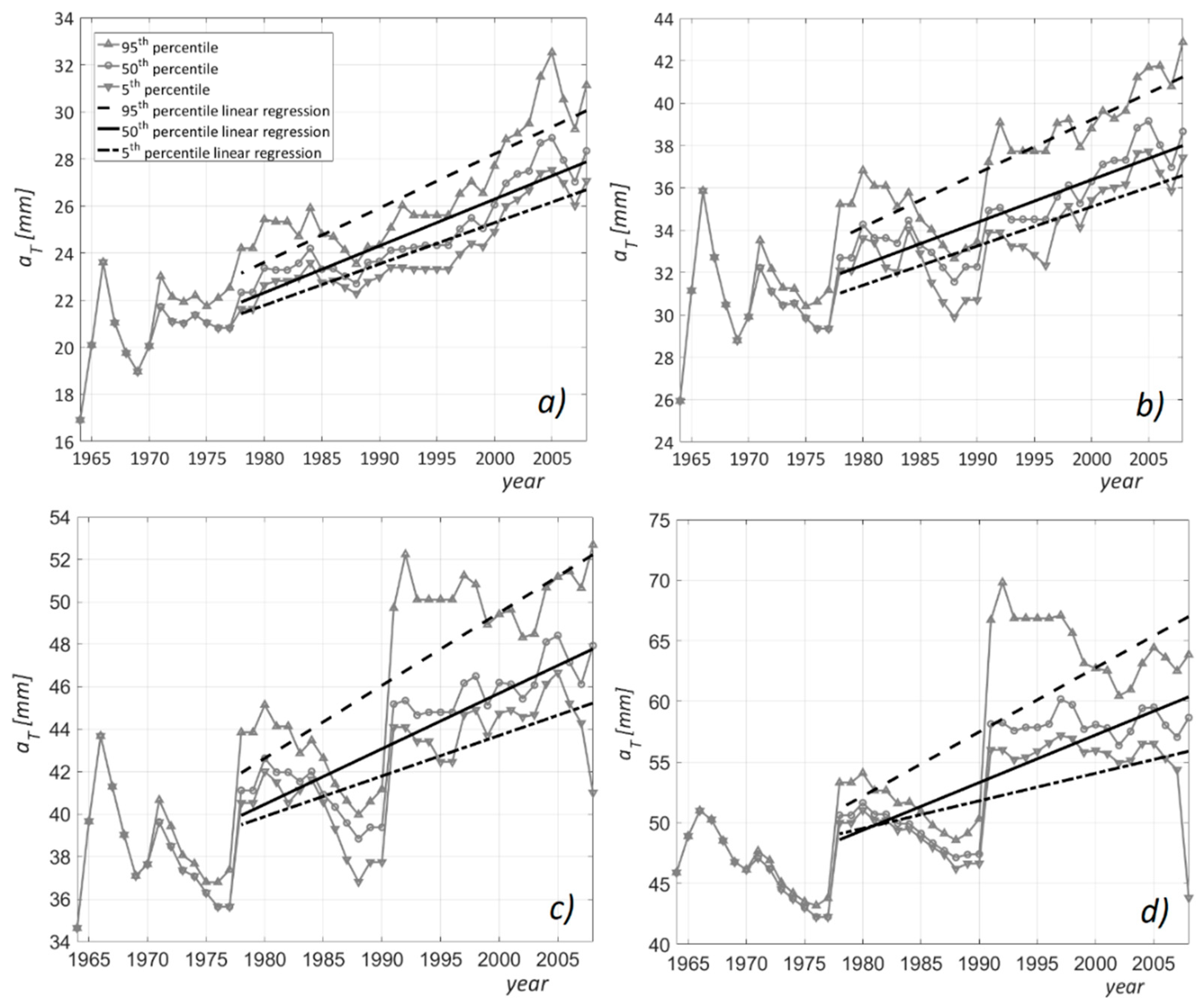
According to Liuzzo et al. [23] the annual maxima rainfall of 1-hour duration recorded in the Piazza Armerina is affected by a statistically significant increasing trend. The application of the Bayesian procedure described in Section 2.2 confirmed this result. Indeed, the linear regression of the aT percentiles showed an increasing trend for each of the considered return periods (Figure 3). The linear regression of the 95th and 5th percentile series delineated the upper and lower limits of the uncertainty bands related to the aT assessment.
Figure 3 shows that, for all the analyzed return periods, the aT 50th percentiles were affected by a quick increase in the last 30 years; nevertheless, the uncertainty bands, delimited by the 95th and the 5th percentiles, were divergent, meaning that the bandwidth was wider for the last years of the examined period compared to the earlier years of the series. This behavior is more emphasized for T equal to 10 and 20 years (Figure 3c,d, respectively) and can be attributed to the higher variability of the 95th percentiles. Specifically, an abrupt change of the 95th percentile can be observed in 1990. The divergence of the 95th and 5th linear regression lines indicates that the uncertainty related to climate change in the assessment of the aT parameter increases over time. Therefore, medium- and long-term future projections will be affected by an increasing level of uncertainty.
The equations of the linear regressions were used to calculate the aT values for the current climate conditions, the 2010 scenario, and for two future short-term projections to 2025 and 2050. Table 1 summarizes the values of the aT parameters for each scenario and return period. In the examined scenarios, variations due to climate change of the scaling exponent nT in Equation (1) were neglected [23].
Focusing on the 50th percentiles, an increase ranging between 8% and 12% can be observed comparing the aT values in the 2010 and the 2025 scenarios. Specifically, the highest increase of aT is assessed in the 2025 scenario for T = 5 years. As regards the 2050 scenario, the aT increase varies between 21% and 28%, with the highest increase for T = 2 years. These increases are comparable to those assessed for the 5th percentiles, whereas the 95th percentiles show slightly higher increases (up to 30% for the 2050 scenario).
The aT parameters in Table 1 were used to calculate the design storm provided as input of the FLO-2D hydraulic simulations. These simulations were performed considering all the aT percentiles for each return period and scenario (36 simulations).
3.2. Maps of Maximum Flow Depths
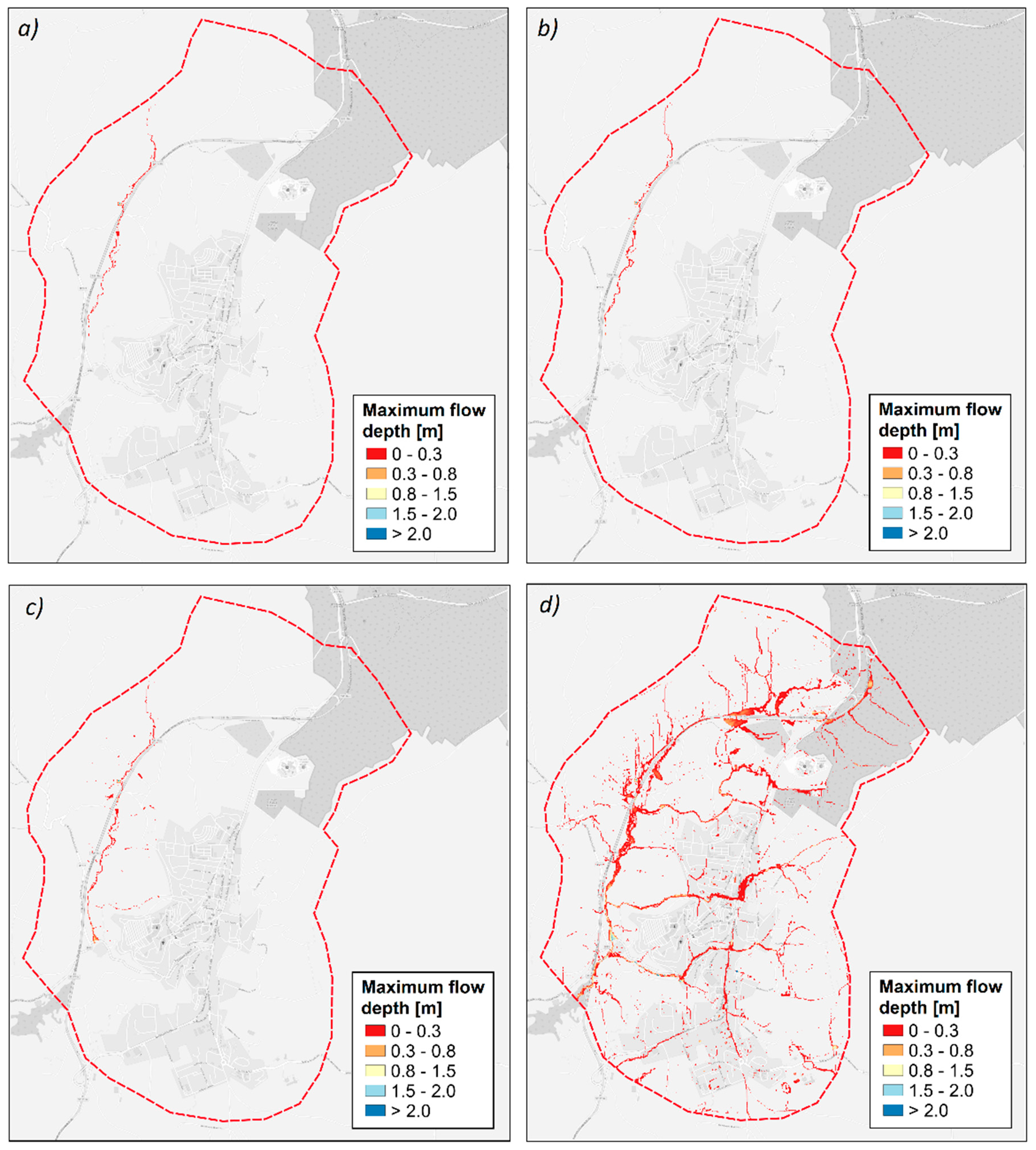
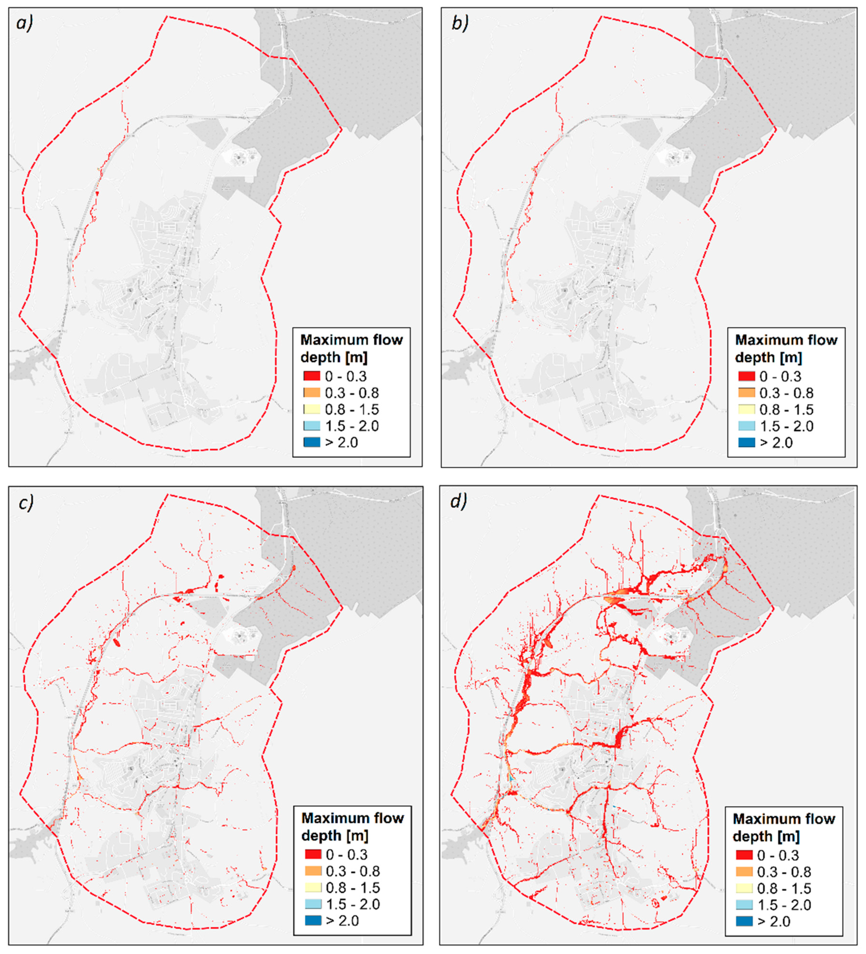
The effects of climate change on the maximum flow depth and the extension of the flooded areas in the urban catchment of Piazza Armerina were investigated. The output of the FLOD-2D simulations was used to obtain some maps in which the maximum flow depth for rainfall events of different return periods was shown. Figure 4 shows the spatial distribution of maximum flood depth for the current climate conditions (2010 scenario). These results were obtained from the hydraulic simulations based on the 50th percentile of aT. For T equal to 2, 5, and 10 years (Figure 4a–c, respectively), flooded areas have a small extension, and the flow depth does not exceed 0.3 m. For T equal to 20 years (Figure 4d), flooded areas are distributed over the whole urban catchment area, and in some locations, maximum flow depths are up to 0.8 m. The percentage of the flooded areas in the urban catchment ranges from 0.17% (for T = 2 years) to 5.48% (for T = 20 years).
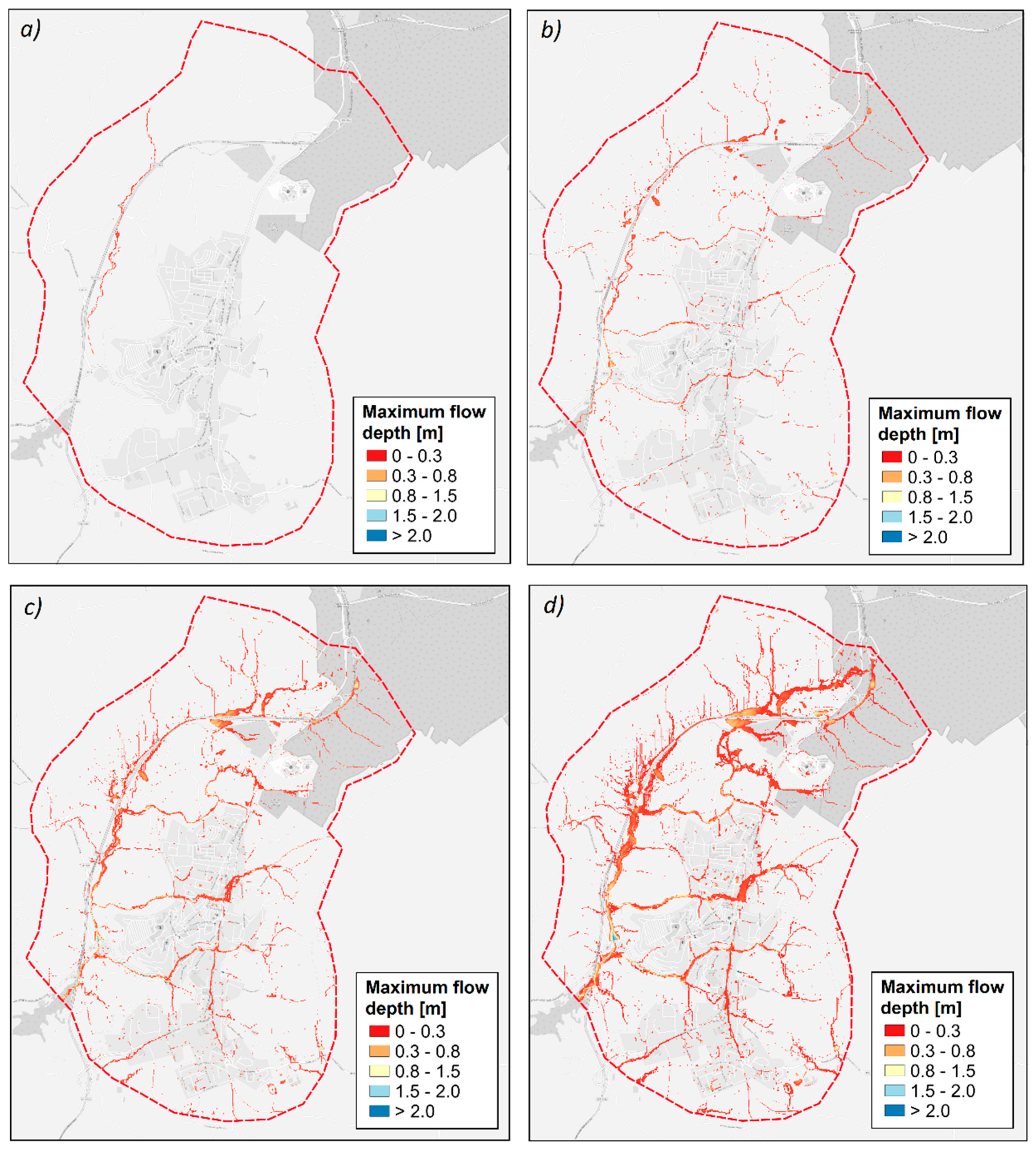
Figure 5 shows the maps of maximum flood depth for the 2025 scenario. For T equal to 2 and 5 (Figure 5a,b, respectively), flooded areas are comparable with those detected for the 2010 scenario. An increase of flooded areas is observed for T equal to 10 years. Further, the spatial distribution of these areas is affected by the increase of rainfall predicted by the Bayesian procedure for 2025. For T equal to 20 years (Figure 5d), maximum flow depths are up to 3 m. The percentage of the flooded areas in the urban catchment ranges from 0.18% (for T = 2 years) to 6.94% (for T = 20 years). In summary, for the 2025 scenario, the effects of climate change are negligible for small return periods, whereas they are more evident for the highest analyzed return periods. Specifically, the comparison of the maps for the 2010 and 2025 scenarios highlights that the increase of annual maximum rainfall has evident implications on flood risk related to events with a 10-year return period.
Figure 6 shows the maps of maximum flood depth for the 2050 scenario. As in the previous future scenario, the increase of rainfall does not affect the maximum flow depth and the extension of the flooded areas for T equal to 2 years (Figure 6a). Nevertheless, in this case, the effects of climate change are already more evident for T equal to 5 years. In Figure 6b, it can be observed that a remarkable increase of flooded areas occurred, if compared with the same maps obtained for the 2010 and the 2025 scenarios. The percentage of the flooded areas in the urban catchment ranges from 0.20% (for T = 2 years) to 8.82% (for T = 20 years). For T equal to 20 years (Figure 6d), the comparison between the maximum flow depth maps for the 2010 and the 2050 scenario highlights significant changes in the extension of the flooded areas. Further, the maximum flow depth area is affected, with an increase of the values up to 1.5 m in many locations.
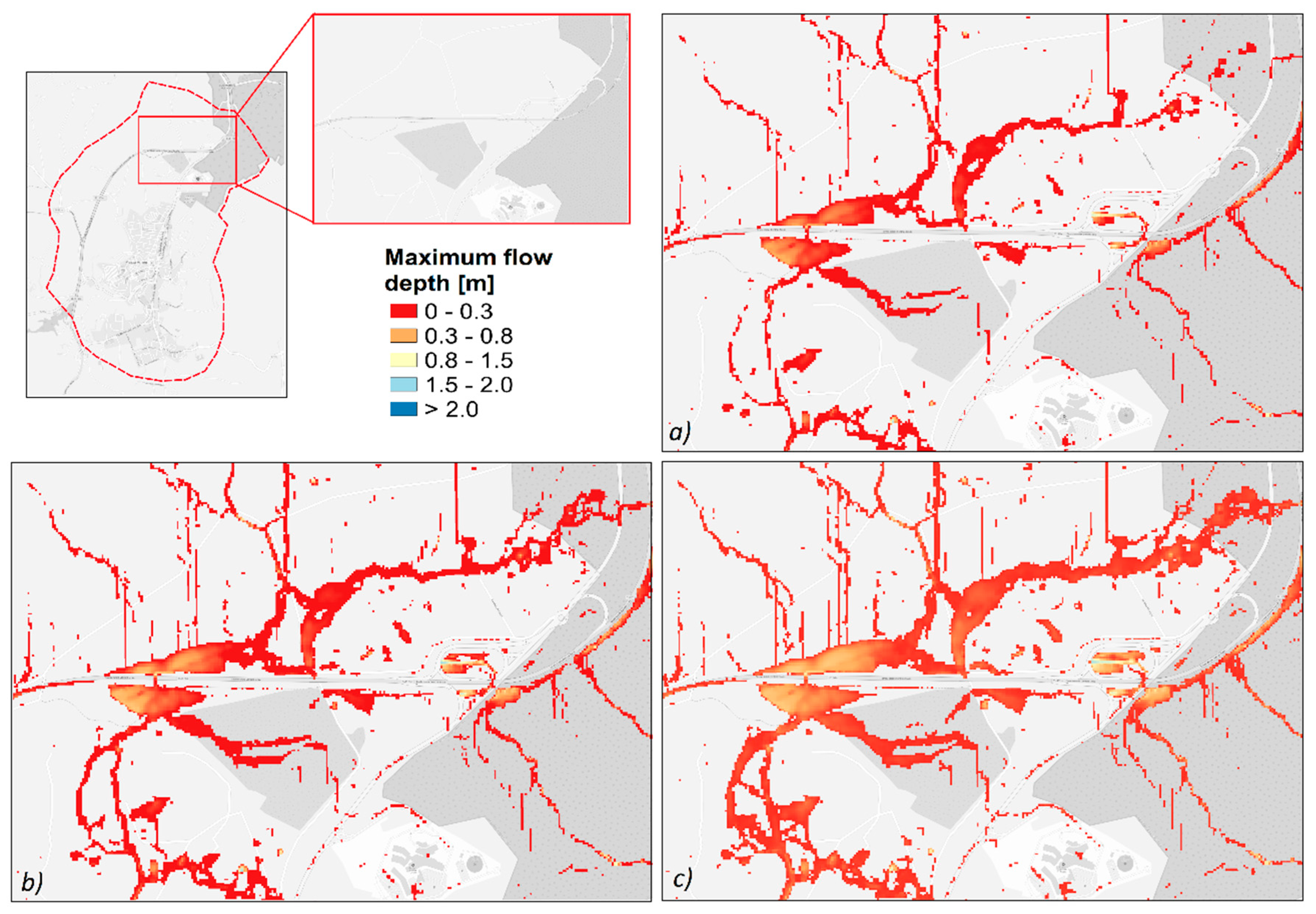
Figure 7 shows the detail of a flood-susceptible area of Piazza Armerina for T = 20 years. Comparing the climate scenarios, an increase of the flooded areas occurs. Wider flooded areas are not the only effect of the rainfall positive trend. Further, an increase of the maximum flow depth can be observed in most of the flooded areas, with values up to 1.5 m. This result highlights that the implication of climate change on extreme rainfall can have important short-term consequences on urban flooding. Basically, rainfall events that in current climate conditions are not particularly severe are likely to become more dangerous in the immediate future.
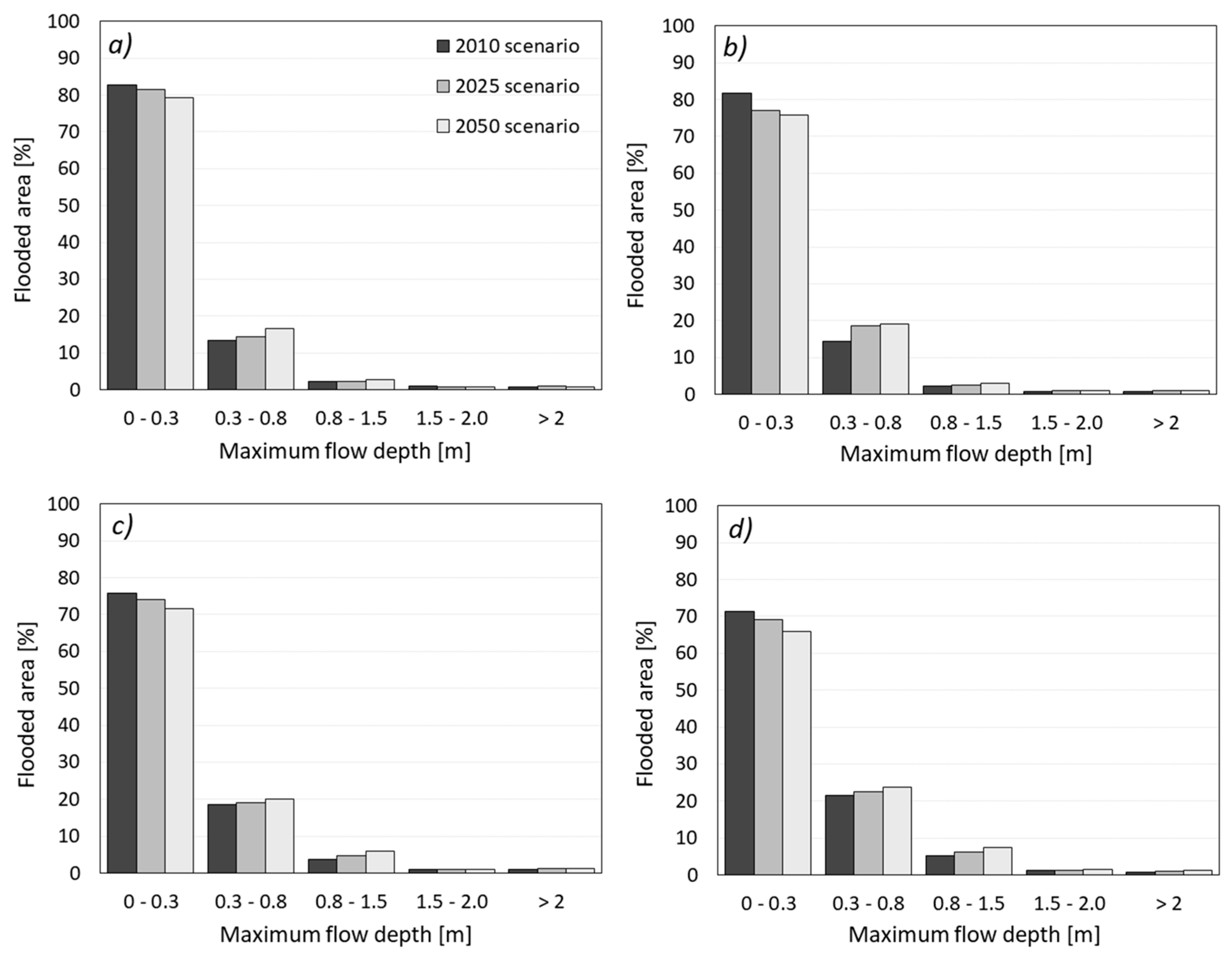
Figure 8 shows the percentage of flooded area for each range of maximum flow depth reported in the previous maps and for each return period. For all the considered return periods and climate scenarios, in most of the flooded area (65–80%), the maximum flow depth ranges between 0 and 0.3 m, whereas a percentage ranging from 12% to 20% of the flooded area is interested by maximum flow depths between 0.3 and 0.8 m. Higher values of maximum flow depth do not exceed 1% of the flooded areas in most cases. Nevertheless, a small increase of the maximum flow depth in the ranges 0.3–0.8 m and 0.8–1.5 m occurs for the 2025 and 2050 scenarios, with a reduction of the percentage of flooded area with the lowest maximum flow depth (0–0.3 m). This effect is not affected by the return period of the rainfall event. These results point out that the positive trend of annual maximum rainfall has consequences not only on the extension of the flooded areas in the urban catchment, but also on the values of the maximum flow depth.
As previously mentioned, the maps of Figure 4, Figure 5 and Figure 6 were obtained from FLO-2D simulations in which the design storm was assessed using the 50th percentile of the aT parameters (Table 1). However, for all the examined return periods, hydraulic simulations were also carried out using the design storm obtained using the DDF curves with 95th and the 5th percentiles of the aT parameters. Results were reported in maps, and the flooded areas were calculated. Assessing the extension of the flooded areas also using the 95th and the 5th percentiles of the aT parameter allowed quantifying the uncertainty related to the estimations illustrated in Figure 4, Figure 5 and Figure 6. Specifically, the maps obtained with the 95th and the 5th percentiles of aT identified the upper and lower limit of the flooded areas, respectively. Basically, the application of the Bayesian procedure for the assessment of the design storms allowed defining a potential range of variation for the flooded areas in climate change scenarios.
Table 2 summarizes the flooded areas for each scenario, return period, and aT percentile. The analysis of these results shows that in the 2010 scenario, for T equal to 2 and 5 years, there are no substantial differences between the flooded areas, and the range of variations identified with the percentiles of aT is very small. This behavior is also observed for the 2025 and the 2050 scenarios, but only when T is equal to 2 years. The uncertainty related to the assessment of flooded areas is increasing with the increase of the return period. Therefore, the uncertainty is minimum for every scenario with T equal to 2 years, while it is maximum for the 2050 scenario when T is equal to 20 years. In this case, there is a difference of 0.54 km2 in the flooded areas assessed with the 95th and the 5th percentiles of the aT parameter.
4. Discussion
In literature, different methodologies have been proposed for the investigation of climate change effects on the performance of urban drainage systems. In this study, the applied approach allowed not only quantifying the variations of flooded areas, but also having a measure of the uncertainty related to these assessments. Results have been reported in some maps in which the maximum flow depths are shown. The comparison between these maps provided an estimation of the increase/decrease of flooded areas due to rainfall variations.
The application of the methodology highlighted some limitations, mainly related to the generation of long-term scenarios. Indeed, the Bayesian procedure only provides the update of the aT parameter for short-term scenarios. In order to obtain more reliable future estimation, the calculation of aT needs to be updated by including any new available data to the original dataset. The addition of new data can affect the detected trend in terms of direction and magnitude. If the procedure were to be applied without the updating of the original dataset, the linear extrapolation approach would lead to an unreliable unlimited rainfall increase.
Another limitation of this study is related to the assumptions made for the climate scenario generation. As previously mentioned, in this study, the temporal analogue approach was used to define some climate scenarios, assuming that the linear variation of precipitation over the past few years will proceed with the same pattern in the future. Clearly, this way of generating climate scenarios can be considered questionable, since climate is a strongly nonlinear system. Nevertheless, the definition of future climate projections requires some assumptions. It has to be remarked that a climate scenario is not intended to explicitly represent the real future climate, but only one of the possible potential realizations. Therefore, caution must be exercised in the interpretation of climate change scenarios.
5. Conclusions
Extreme rainfall variations due to climate change are expected to have remarkable implications on the magnitude and frequency of peak flows over the service life of urban drainage systems. For this reason, the assessment of the design storm became a critical issue. Specifically, current guidelines and methodologies for the design of urban drainage systems need to be improved and updated to incorporate the effects of climate change in the evaluation of the design storm. Moreover, the uncertainty related to this estimation needs to be assessed and quantified.
In this work, a Bayesian procedure was applied to estimate the aT parameter of the DDF curves in some climate change scenarios. These curves were used as input of the FLO-2D model to evaluate and quantify the effects of extreme rainfall variations on urban flooding in Piazza Armerina, a small town located in Southern Italy. In this area, the annual maximum rainfall increased during the 1956–2008 period. The parameters of the DDF curves were updated to take into account this positive trend in two short-term climate projection at 2025 and 2050. The implications of the rainfall increase on the performance of the urban drainage system of Piazza Armerina were investigated, comparing the maximum flow depths and the flooded areas assessed for the current climate conditions (scenario 2010) with those of the 2025 and 2050 scenarios. The analysis was performed considering the design storm of the 2-, 5-, 10-, and 20-year return period. A total of 36 hydraulic simulations were carried out. Results showed that the effect of the rainfall trend is more significant for the flooding related to events with 10- and 20-year return periods. The application of the Bayesian procedure for the assessment of the DDF curve parameters allowed quantifying the uncertainty due to rainfall change related to the definition of the design storm and, consequently, the identification of the flooded areas in the examined urban catchment.
Author Contributions
Conceptualization, L.L. and G.F.; data curation, L.L. and G.F.; formal analysis, L.L. and G.F.; investigation, L.L. and G.F.; methodology, L.L. and G.F.; writing—original draft preparation, L.L. and G.F.; writing—review and editing, L.L. and G.F.; visualization, L.L. and G.F.; supervision, G.F.
Funding
This research received no external funding.
Conflicts of Interest
The authors declare no conflict of interest.
References
- Portmann, R.W.; Solomon, S.; Hegerl, G.C. Spatial and seasonal patterns in climate change, temperatures, and precipitation across the United States. Proc. Natl. Acad. Sci. USA 2009, 106, 7324–7329. [Google Scholar] [CrossRef] [PubMed] [Green Version]
- Donat, M.G.; Alexander, L.V.; Yang, H.; Durre, I.; Vose, R.; Dunn, R.J.H.; Hewitson, B. Updated analyses of temperature and precipitation extreme indices since the beginning of the twentieth century: The HadEX2 dataset. J. Geophys. Res. Atmos. 2013, 118, 2098–2118. [Google Scholar] [CrossRef]
- Westra, S.; Alexander, L.V.; Zwiers, F.W. Global increasing trends in annual maximum daily precipitation. J. Clim. 2013, 26, 3904–3918. [Google Scholar] [CrossRef]
- Arisz, H.; Burrell, B.C. Urban drainage infrastructure planning and design considering climate change. In Proceedings of the 2006 IEEE EIC Climate Change Conference, Ottawa, ON, Canada, 10–12 May 2006. [Google Scholar]
- Arnbjerg-Nielsen, K.; Fleischer, H.S. Feasible adaptation strategies for increased risk of flooding in cities due to climate change. Water Sci. Technol. 2009, 60, 273–281. [Google Scholar] [CrossRef] [PubMed]
- Freni, G.; La Loggia, G.; Notaro, V. Uncertainty in urban flood damage assessment due to urban drainage modelling and depth-damage curve estimation. Water Sci. Technol. 2010, 61, 2979–2993. [Google Scholar] [CrossRef]
- Arnbjerg-Nielsen, K.; Willems, P.; Olsson, J.; Beecham, S.; Pathirana, A.; Bülow Gregersen, I.; Madsen, H.; Nguyen, V.-T.-V. Impacts of climate change on rainfall extremes and urban drainage systems: A review. Water Sci. Technol. 2013, 68, 16–28. [Google Scholar] [CrossRef]
- Schreider, S.Y.; Smith, D.I.; Jakeman, A.J. Climate change impacts on urban flooding. Clim. Chang. 2000, 47, 91–115. [Google Scholar] [CrossRef]
- Denault, C.; Millar, R.G.; Lence, B.J. Assessment of possible impacts of climate change in an urban catchment. J. Am. Water Res. Assoc. 2006, 42, 685–697. [Google Scholar] [CrossRef]
- Markus, M.; Wuebbles, D.J.; Liang, X.Z.; Hayhoe, K.; Kristovich, D.A. Diagnostic analysis of future climate scenarios applied to urban flooding in the Chicago metropolitan area. Clim. Chang. 2012, 111, 879–902. [Google Scholar] [CrossRef]
- Huong, H.T.L.; Pathirana, A. Urbanization and climate change impacts on future urban flooding in Can Tho city, Vietnam. Hydrol. Earth Syst. Sci. 2013, 17, 379–394. [Google Scholar] [CrossRef] [Green Version]
- Zhou, Q.; Leng, G.; Huang, M. Impacts of future climate change on urban flood volumes in Hohhot in northern China: Benefits of climate change mitigation and adaptations. Hydrol. Earth Syst. Sci. 2018, 22, 305–316. [Google Scholar] [CrossRef]
- Da Silva, C.; Schardong, A.; Garcia, J.; Oliveira, C. Climate change impacts and flood control measures for highly developed urban watersheds. Water 2018, 10, 829. [Google Scholar] [CrossRef]
- Andimuthu, R.; Kandasamy, P.; Mudgal, B.V.; Jeganathan, A.; Balu, A.; Sankar, G. Performance of urban storm drainage network under changing climate scenarios: Flood mitigation in Indian coastal city. Sci. Rep. 2019, 9, 7783. [Google Scholar] [CrossRef] [PubMed]
- Olsson, J.; Berggren, K.; Olofsson, M.; Viklander, M. Applying climate model precipitation scenarios for urban hydrological assessment: A case study in Kalmar City, Sweden. Atmos Res. 2009, 92, 364–375. [Google Scholar] [CrossRef]
- Kaspersen, P.S.; Ravn, N.H.; Arnbjerg-Nielsen, K.; Madsen, H.; Drews, M. Influence of urban land cover changes and climate change for the exposure of European cities to flooding during high-intensity precipitation. Proc. IAHS 2015, 370, 21–27. [Google Scholar] [CrossRef] [Green Version]
- Ashley, R.; Tait, S.; Cashman, A.; Blanksby, J.; Hurley, A.L.; Sandlands, L.; Saul, A. 21st Sewerage Design; Full Report, UKWIR Report 06/WM07/7; UK Water Industry Research: London, UK, 2006. [Google Scholar]
- Abdellatif, M.; Atherton, W.; Alkhaddar, R.; Osman, Y. Flood risk assessment for urban water system in a changing climate using artificial neural network. Nat Hazards 2015, 79, 1059–1077. [Google Scholar] [CrossRef]
- Willems, P.; Arnbjerg-Nielsen, K.; Olsson, J.; Nguyen, V.T.V. Climate change impact assessment on urban rainfall extremes and urban drainage: Methods and shortcomings. Atmos. Res. 2012, 103, 106–118. [Google Scholar] [CrossRef]
- Archetti, R.; Bolognesi, A.; Casadio, A.; Maglionico, M. Development of flood probability charts for urban drainage network in coastal areas through a simplified joint assessment approach. Hydrol. Earth Syst. Sci. 2011, 15, 3115–3122. [Google Scholar] [CrossRef] [Green Version]
- Krasovskaia, I.; Gottschalk, L. Stability of river flow regimes. Hydrol. Res. 1992, 23, 137–154. [Google Scholar] [CrossRef]
- Notaro, V.; Liuzzo, L.; Freni, G.; La Loggia, G. Uncertainty analysis in the evaluation of extreme rainfall trends and its implications on urban drainage system design. Water 2015, 7, 6931–6945. [Google Scholar] [CrossRef]
- Liuzzo, L.; Notaro, V.; Freni, G. Uncertainty related to climate change in the assessment of the DDF curve parameters. Environ. Model. Softw. 2017, 96, 1–13. [Google Scholar] [CrossRef]
- O’Brien, J.S.; Julien, P.Y.; Fullerton, W.T. Two-Dimensional Water Flood and Mudflow Simulation. J. Hydraul. Eng. 1993, 119, 244–261. [Google Scholar] [CrossRef]
- Liuzzo, L.; Freni, G. Analysis of extreme rainfall trends in Sicily for the evaluation of depth-duration-frequency curves in climate change scenarios. J. Hydrol. Eng. 2015, 20, 04015036. [Google Scholar] [CrossRef]
- Notaro, V.; Fontanazza, C.M.; Freni, G.; La Loggia, G. Assessment of Modelling Structure and Data Availability Influence on Urban Flood Damage Modelling Uncertainty. Procedia Eng. 2014, 89, 788–795. [Google Scholar] [CrossRef] [Green Version]
- Vose, R.S.; Easterling, D.R.; Gleason, B. Maximum and minimum temperature trends for the globe: An update through 2004. Geophys. Res. Lett. 2005, 32. [Google Scholar] [CrossRef] [Green Version]
- Liuzzo, L.; Bono, E.; Sammartano, V.; Freni, G. Analysis of spatial and temporal rainfall trends in Sicily during the 1921–2012 period. Theor. Appl. Climatol. 2016, 126, 113–129. [Google Scholar] [CrossRef]
- Glantz, M. Societal Responses to Climate Change: Forecasting by Analogy, No. 35; Westview Press: Boulder, CO, USA, 1988. [Google Scholar]
Figure 1.
(a) Orthoimage of the area of study; (b) location of the urban drainage main pipes in the area of study.
Figure 1.
(a) Orthoimage of the area of study; (b) location of the urban drainage main pipes in the area of study.

Figure 2.
Flow chart of the applied procedure.

Figure 3.
The 95th, 50th, and 5th percentiles of the aT parameter and linear regressions for different return periods T: (a) 2 years; (b) 5 years; (c) 10 years; and (d) 20 years.
Figure 3.
The 95th, 50th, and 5th percentiles of the aT parameter and linear regressions for different return periods T: (a) 2 years; (b) 5 years; (c) 10 years; and (d) 20 years.

Figure 4.
Maximum flow depth for the 2010 scenario: (a) T = 2 years; (b) T = 5 years; (c) T = 10 years; and (d) T = 20 years.
Figure 4.
Maximum flow depth for the 2010 scenario: (a) T = 2 years; (b) T = 5 years; (c) T = 10 years; and (d) T = 20 years.

Figure 5.
Maximum flow depth for the 2025 scenario: (a) T = 2 years; (b) T = 5 years; (c) T = 10 years; and (d) T = 20 years.
Figure 5.
Maximum flow depth for the 2025 scenario: (a) T = 2 years; (b) T = 5 years; (c) T = 10 years; and (d) T = 20 years.

Figure 6.
Maximum flow depth for the 2050 scenario: (a) T = 2 years; (b) T = 5 years; (c) T = 10 years; and (d) T = 20 years.
Figure 6.
Maximum flow depth for the 2050 scenario: (a) T = 2 years; (b) T = 5 years; (c) T = 10 years; and (d) T = 20 years.

Figure 7.
Detail of a flooded urban area in Piazza Armerina for T = 20 years: (a) 2010 scenario; (b) 2025 scenario; and (c) 2050 scenario.
Figure 7.
Detail of a flooded urban area in Piazza Armerina for T = 20 years: (a) 2010 scenario; (b) 2025 scenario; and (c) 2050 scenario.

Figure 8.
Percentage of flooded areas for each range of maximum flow depths (m): (a) T = 2 years; (b) T = 5 years; (c) T = 10 years; and (d) T = 20 years.
Figure 8.
Percentage of flooded areas for each range of maximum flow depths (m): (a) T = 2 years; (b) T = 5 years; (c) T = 10 years; and (d) T = 20 years.


Table 1.
Parameters nT and aT of depth–duration–frequency (DDF) curves for each scenario and return period T.
Table 1.
Parameters nT and aT of depth–duration–frequency (DDF) curves for each scenario and return period T.
| T (Years) | Scenario | nT | aT (mm) | ||
|---|---|---|---|---|---|
| 95th Percentile | 50th Percentile | 5th Percentile | |||
| 2 | 2010 | 0.27 | 30.5 | 28.3 | 27.0 |
| 2025 | 0.27 | 34.0 | 31.3 | 29.7 | |
| 2050 | 0.27 | 39.7 | 36.2 | 34.1 | |
| 5 | 2010 | 0.32 | 41.7 | 38.4 | 37.0 |
| 2025 | 0.32 | 45.5 | 41.4 | 39.7 | |
| 2050 | 0.32 | 51.9 | 46.4 | 44.4 | |
| 10 | 2010 | 0.29 | 52.9 | 48.3 | 45.6 |
| 2025 | 0.29 | 58.1 | 52.2 | 48.5 | |
| 2050 | 0.29 | 66.6 | 58.8 | 53.2 | |
| 20 | 2010 | 0.29 | 68.0 | 61.1 | 56.3 |
| 2025 | 0.29 | 76.0 | 67.0 | 59.7 | |
| 2050 | 0.29 | 89.2 | 76.8 | 65.4 | |
Table 2.
Flooded area for each scenario, return period, and percentile of the aT parameter.
| Scenario | Return Period (Years) | Flooded Area (km2) | ||
|---|---|---|---|---|
| 95th Percentile | 50th Percentile | 5th Percentile | ||
| 2010 | 2 | 0.020 | 0.019 | 0.018 |
| 5 | 0.042 | 0.021 | 0.020 | |
| 10 | 0.274 | 0.034 | 0.025 | |
| 20 | 0.788 | 0.603 | 0.441 | |
| 2025 | 2 | 0.021 | 0.020 | 0.019 |
| 5 | 0.164 | 0.029 | 0.024 | |
| 10 | 0.507 | 0.243 | 0.094 | |
| 20 | 0.788 | 0.764 | 0.556 | |
| 2050 | 2 | 0.023 | 0.022 | 0.021 |
| 5 | 0.472 | 0.225 | 0.111 | |
| 10 | 0.750 | 0.523 | 0.276 | |
| 20 | 1.258 | 0.970 | 0.719 | |
© 2019 by the authors. Licensee MDPI, Basel, Switzerland. This article is an open access article distributed under the terms and conditions of the Creative Commons Attribution (CC BY) license (http://creativecommons.org/licenses/by/4.0/).
Share and Cite
MDPI and ACS Style
Liuzzo, L.; Freni, G. Quantifying the Uncertainty Related to Climate Change in the Assessment of Urban Flooding—A Case Study. Water 2019, 11, 2072. https://doi.org/10.3390/w11102072
AMA Style
Liuzzo L, Freni G. Quantifying the Uncertainty Related to Climate Change in the Assessment of Urban Flooding—A Case Study. Water. 2019; 11(10):2072. https://doi.org/10.3390/w11102072
Chicago/Turabian StyleLiuzzo, Lorena, and Gabriele Freni. 2019. "Quantifying the Uncertainty Related to Climate Change in the Assessment of Urban Flooding—A Case Study" Water 11, no. 10: 2072. https://doi.org/10.3390/w11102072
Note that from the first issue of 2016, this journal uses article numbers instead of page numbers. See further details here.