Multi-Parametrical Tool for the Design of Bottom Racks DIMRACK—Application to Small Hydropower Plants in Ecuador

Abstract

A novel computational tool, DIMRACK, is presented for the design of the required length of bottom racks in intake systems. The users may consider clear water cases or the rack’s occlusion due to sediment transport in the river. The computational tool uses a methodology based on the experimental works undertaken at the Universidad Politécnica de Cartagena from 2010. This work also presents an extension of the methodology to cover a broad range of void ratios, bar profiles, slopes, and flow rates. Designing nomograms are also proposed. These are two diagrams to allow the approximate graphical computation of the rack length with clear water. In sediment transport cases, an occlusion factor is proposed, obtained from experimental gravel tests. This parameter enables an increment in the rack length due to occlusion, depending on the bar type. The results are compared with those proposed in classical technical manuals. Finally, the results have been compared with ten existing small hydropower plants’ bottom intake designs in Ecuador.

1. Introduction

In 2018, approximately 81% of the electricity consumed in Ecuador came from hydroelectric energy. About 21,000 GWh were generated in the hydroelectric plants owned by the government during that year, according to the National Energy Operator (CENACE) [1]. Several studies dealing with hydroelectric power plants have been developed in Ecuador. From these, around twelve include small hydropower plants (SHP), i.e., with an installed capacity below 10 MW. Small hydropower has been identified as one of the important energy sources that can provide convenient and uninterrupted energy to remote rural communities or industries [2]. Bottom racks were proposed for the water intakes of all these SHP. The racks are designed to be put in the stream bed in order to derive part of the stream flowrate and to avoid solids larger than the space between the bars from entering.

Table 1. Characteristics of the small hydropower plants (SHP) planned in mountain rivers in Ecuador [3,4,5,6].

Name	Head (m)	Installed Capacity (MW)	Estimated Annual Production (GWh/year)	Turbines
Dudas [3]	294.00	7.40	41.35	1 Pelton unit
San Antonio [3]	195.00	7.19	44.87	1 Pelton unit
Jondachi-Sardinas [4]	98.77	6.71	44.06	2 Francis units
Nanegal [5]	110.00	5.30	37.16	2 Francis units
Alambi [5] *	110.00	5.50	29.50	2 Francis units
Tulipe [5]
Chuquiraguas [5]	300.00	2.35	13.15	2 Pelton units
Chanchán [5]	220.00	7.25	38.78	3 Pelton units
Chalpi A [6] **	398.62	7.67	24.70–35.96 (depending on urban water supply requirements)	2 Pelton units
Encantado [6]
Chalpi B [6]
Chalpi C [6]

Notes: * Alambi and Tulipe intakes belong to same SHP; ** Chalpi A, Encantado, Chalpi B, and Chalpi C belong to same SHP.

summarizes the characteristics of these intakes designed by different administrations and universities in Ecuador [3,4,5,6].

As case study examples, the details of Chalpi A, Dudas, and San Antonio bottom intakes can be seen in Figure 1 and Figure 2. These projects are currently under construction.

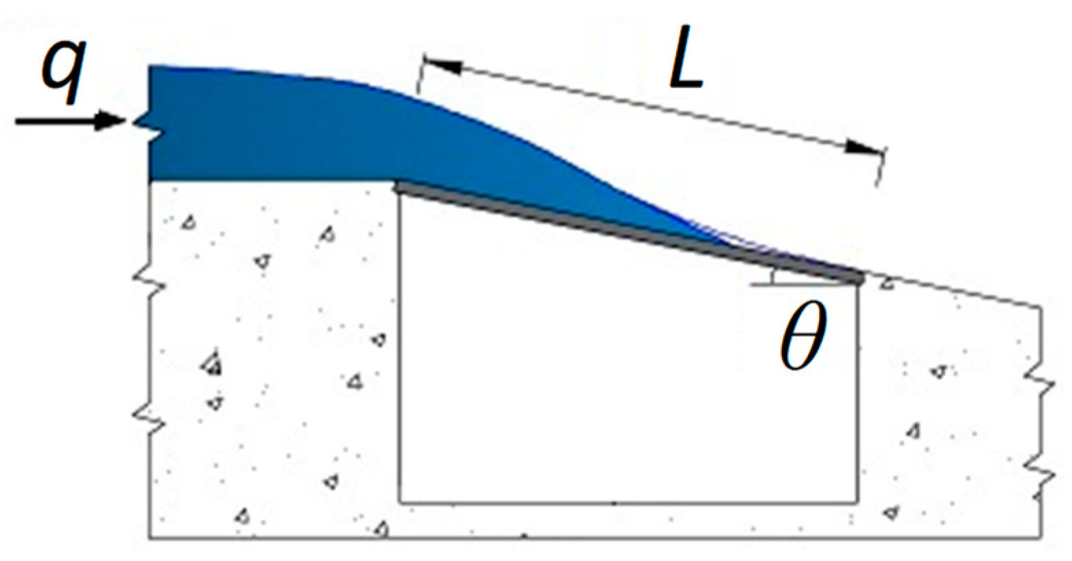
From the beginning of the 20th century, many researchers have investigated bottom racks in the laboratory and in the field to obtain the design parameters for these intakes. The rack length to derive a certain flow is its main objective. In each case, the bar type - with a predomination of T-shaped, prismatic, circular, and top-rounded -, the space between bars, and the longitudinal slope of the racks, give rise to important differences in the length of the rack [7,8,9,10,11,12]. Figure 3 presents a scheme of the configuration of these intakes, where q is the approximation flowrate to derive, tanθ the longitudinal slope, and L the rack length necessary to completely derive the flow.

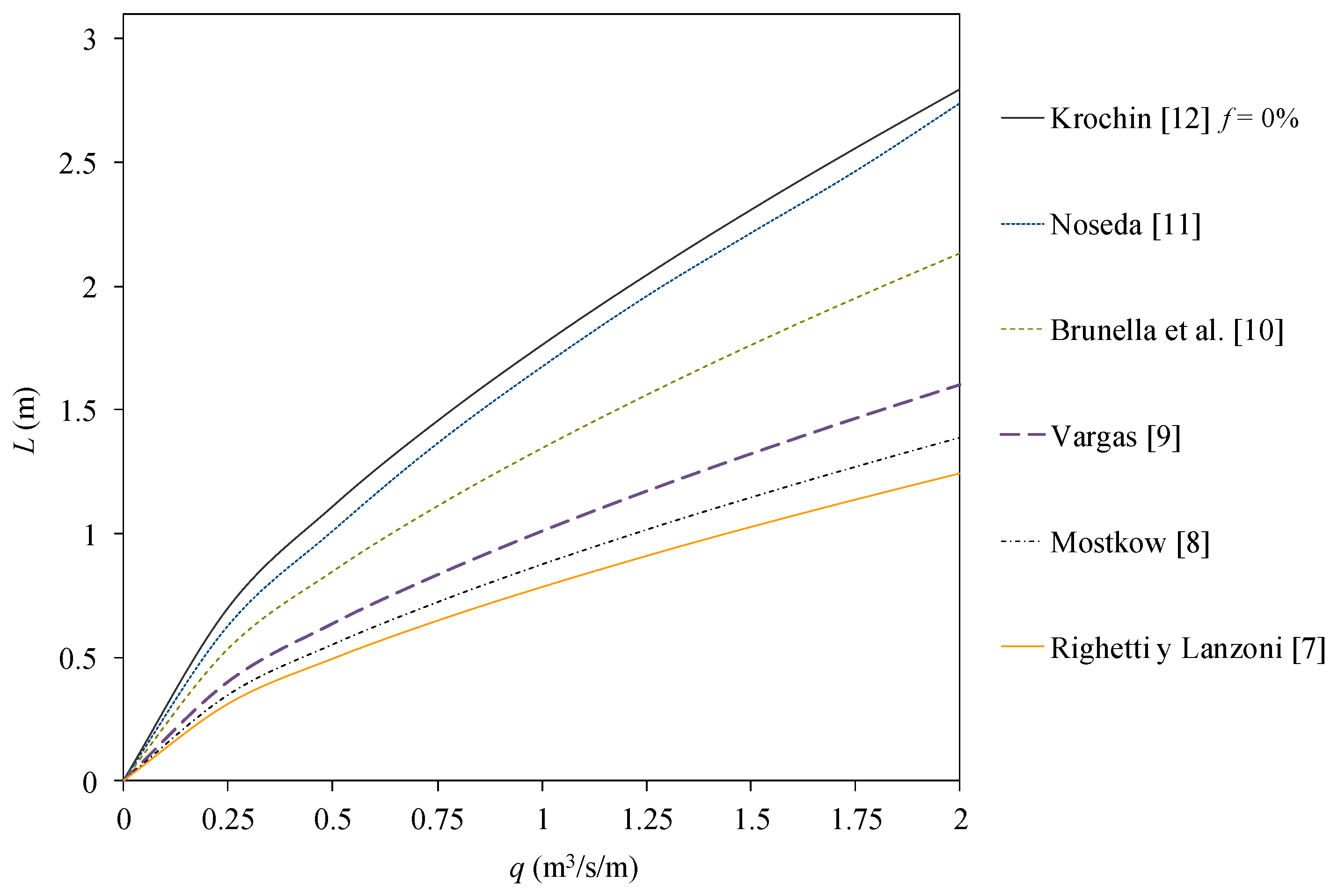
Figure 4 presents the length of the rack, calculated according to the proposals of several studies, in the case of a void ratio (area of void divided by the total area of the rack), m = 0.60, and longitudinal slope of 20%. In the figure, the differences between the values proposed are over 100%, which makes it difficult to choose a design value. This is due to the different configurations of the experiments taken by each researcher, which give rise to important differences. Those differences can be observed in

Table 2. Different setups of experiments to define the length of the bottom racks for q₁ = 1.25 m³/s/m.

Autor	Required Length (m)	Shape of the Bars	Setting of the Rack, Void Ratio	Slope of the Experiments
Righetti & Lanzoni [7]	0.91	Prismatic with rounded edge	m = 0.20; b1 = 0.50 cm; bw = 2.00 cm	<3.5%
Mostkow [8]	1.01	Prismatic	Not specified
Vargas [9]	1.17	Circular	Two setups: (a) m = 0.33; b1 = 0.50 cm; bw = 1 cm; (b) m = 0.5; b1 = 1 cm; bw = 1 cm	slope: 0°–20°
Brunella et al. [10]	1.56	Circular	Two setups: (a) b1 = 0.60 or 0.30 cm; bw = 1.20 or 0.60 cm; m = 0.352 (b) b1 = 1.80 or 0.90 cm; bw = 1.20 or 0.60 cm; m = 0.664	0°–51°
Noseda [11]	1.96	T- shaped	0.16 < m < 0.28 0.57 < b1 < 1.17 cm	0–20%
Krochin [12] f = 0%	2.04	Prismatic	Not specified

Notes: b₁ is the space between bars; b_w the width of a bar; and $m=b_1/\left(b_1+b_w\right)$ the void ratio.

for the specific flowrate of q = 1.25 m³/s/m. In all the cases, an occlusion factor f = 0 was considered. The parameter f multiplies the wetted rack length calculated with a clear water hypothesis.

In 1981, Drobir [13] proposed the first technical guide for the design of the bottom intake racks. This was based on experiences in the management of several bottom intakes from TIWAG Tyrolean hydroelectrical company and the proposals of Frank [14], which were in agreement with the experimental values presented by Noseda [11]. In view of the abacus proposed in the technical manual, m adopts a single value equal to 0.60. The equations proposed by Frank [14,15] are included below.

$$q=\raisebox{1ex}{$2$}\!\left/ \!\raisebox{-1ex}{$3$}\right.c{C}_{q0}L\sqrt{2g{h}_0}$$

(1)

$$h_0=k_c{h}_c$$

(2)

$$c=0.6m{\left(\cos \beta \right)}^{\raisebox{1ex}{$3$}\!\left/ \!\raisebox{-1ex}{$2$}\right.}$$

(3)

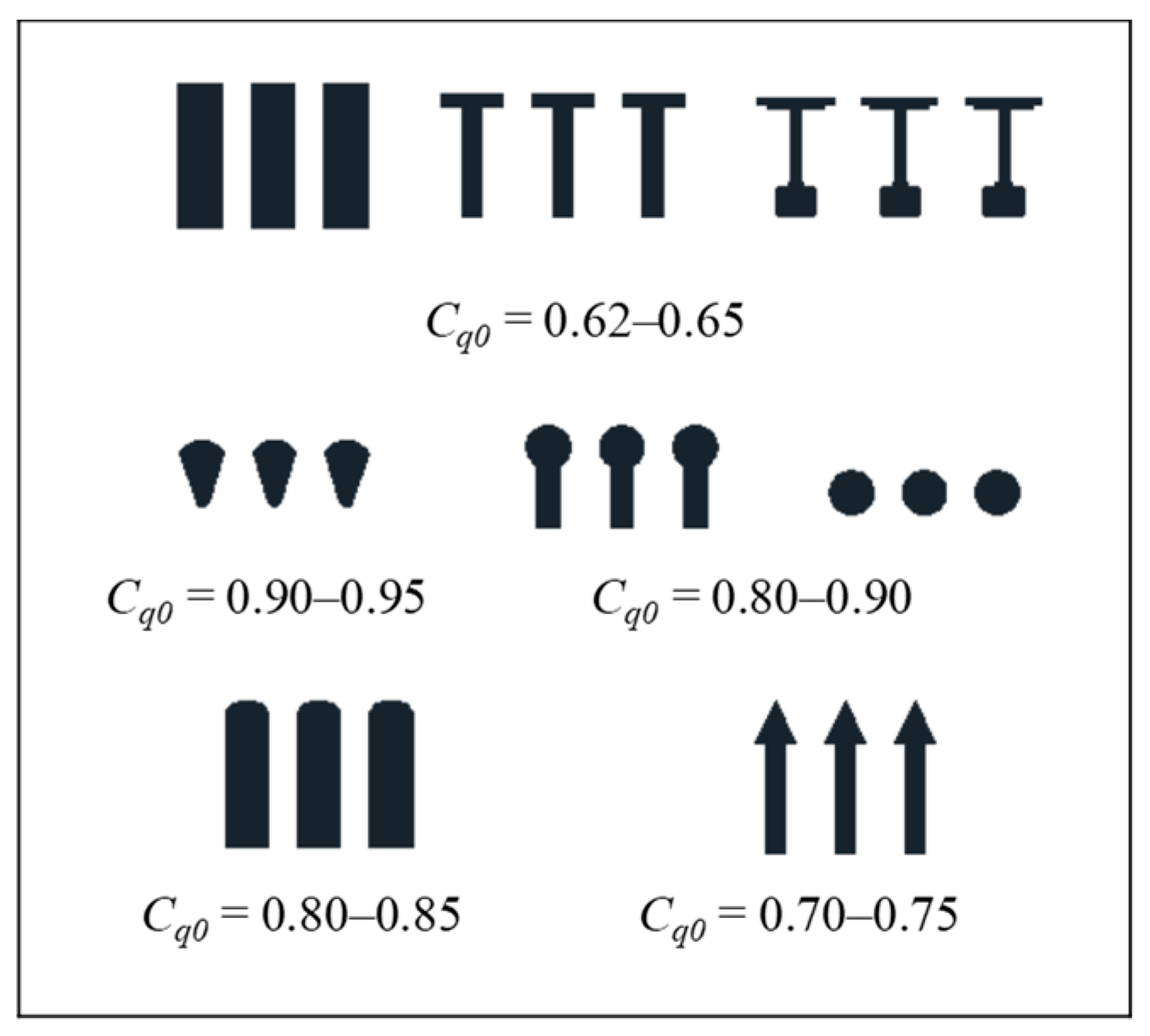
where q is the specific flowrate to derive (m³/s/m); C_q0 the discharge coefficient measured in racks with m = 0.60 in static conditions, i.e., with still flow dissipating the kinetic energy [7,8,10,16] (-); L is the wetted rack length to be calculated (m); h₀ the flow depth at the beginning of the rack (m); k_c a coefficient to correct the flow depth at the beginning of the rack depending on the longitudinal slope [14,15] (-); h_c the critical depth calculated as $h_c={\left(q/\sqrt{g}\right)}^{2/3}$ (m); and g the gravity acceleration (m/s²). Figure 5 shows the values of the static discharge coefficients proposed by Frank.

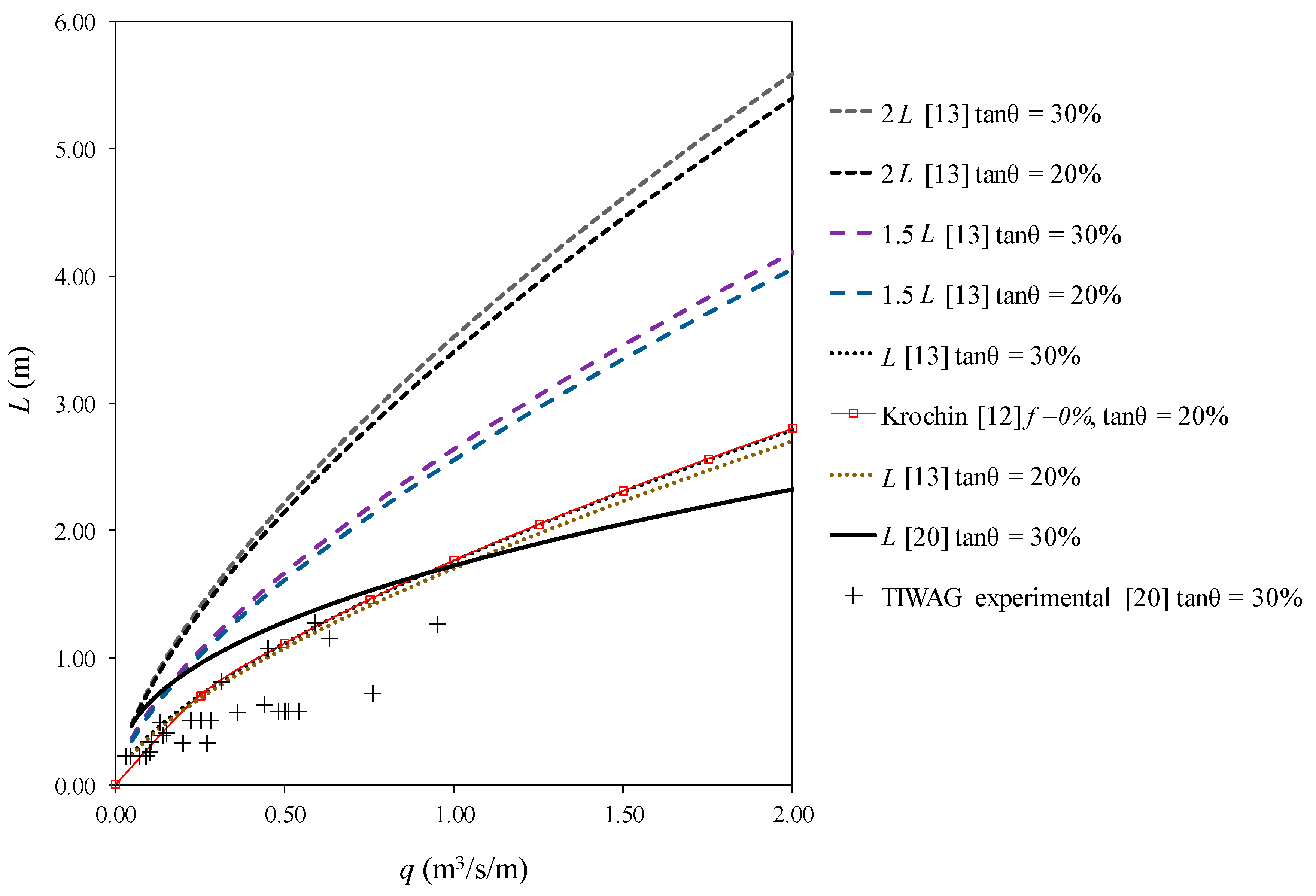
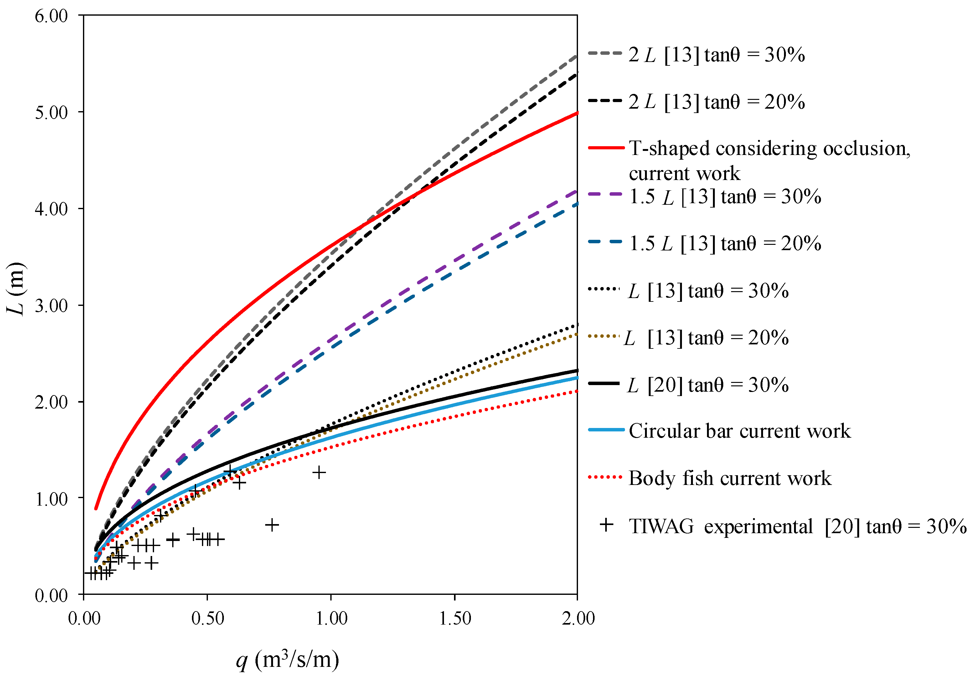
Other technical manuals such as those by Lauterjung and Schmidt [18] and Andaroodi and Schleiss [2] also include the methodology proposed by Frank, summarized by Equations (1)–(3). All of them proposed an increment in the calculated wetted rack length, L, to consider the occlusion of the space between the bars due to the sediments transported with the river flows. While Drobir [13,19] proposed increment values between 50% and 100%, other authors [2,18] proposed increments of around 20%. In parallel, Krochin [12] gathered the experience in bottom intakes from the east of Europe and took it to Ecuador. That author proposed occlusion factors of 15% and 30% of increment, and recommended the use of prismatic bars, differing from the TIWAG experiences that proposed more hydrodynamic bars, such as the case of circular and fish body profiles. In 1999, Drobir [20] obtained field measurements in a prototype at the Kaunertal power plant managed by the TIWAG. Measurements were taken in a bottom intake with the void ratio of m = 0.60, circular bars, and a longitudinal slope of 20%. Drobir [20] proposed a novel potential adjustment for the rack length as an envelope of all field measurements, improving though the previous knowledge from Frank [14,15]. The distinction between the behavior of the wetted rack length, which is more gravitational, and the other, more influenced by the surface tension, was first introduced by [20]. Figure 6 presents the rack length proposed by those authors [12,13,20]. It can be observed that the shape of the length curve, once it has been improved by Drobir’s field measurements [20], is more horizontal than previous designs. This is due to the important influence of the end part of the wetted length, characterized by low flows governed by surface tension around the bars that gives rise to quite constant lengths. This end part of the wetted length had not been well identified previously [13,14,15]. In Figure 6 we can observe the agreement between the length proposed by Krochin [12], considering an occlusion factor f = 0% and prismatic bars, and that proposed by Frank [14,15], published in [13]. with fish body and circular bars, both for the longitudinal slope of tanθ = 20%. Figure 6 also includes the recommendations in [13] to consider 1.5 and two times the calculated length by Frank [14,15], to take occlusion of the racks into account.

This work is based on the experimental work developed at the Universidad Politécnica de Cartagena from 2010 [16,21,22,23,24,25,26,27,28,29,30,31], presenting an extension of a methodology [25] to calculate the length of the rack considering different bar profiles and void ratios, beyond those proposed in previous technical manuals [2,12,13,18,20]. This includes clear water and flow, with gravel tests that enable the increment of the length due to occlusion to be assessed. The results are compared with those proposed by Frank [14,15] and Drobir [13,20]. Comparison with ten existing SHP bottom intake designs in Ecuador [4,5,6] are also studied and discussed in the present work. A series of designing nomograms are proposed. These are two nondimensional diagrams to allow the approximate graphical computation of the rack length. To finish, a computational tool created in Matlab^® software and available online, DIMRACK, gathers together all the conclusions and serves as a Tool for the Design of Bottom Racks with the possibility of taking into account multiple different parameters such as different void ratios, bar types, longitudinal slope, and flowrates.

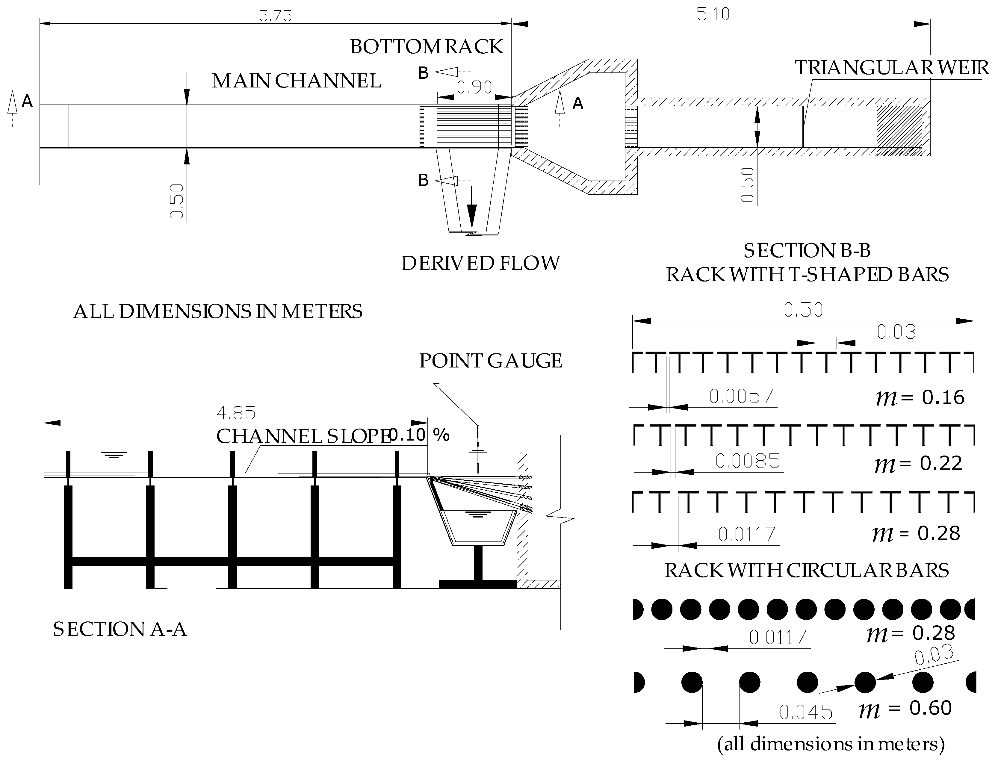
2. Experimental Setting

The physical device consists of an intake system based on Noseda’s [11] physical model (Figure 7). The inlet is a 5.00 m long and 0.50 m wide channel with methacrylate walls. At the end of the channel there is a bottom rack intake system with different slopes (from horizontal to 33%). The racks were built with aluminium bars with T-shaped flat and circular profiles. The rack is 0.90 m long in the flow direction. Bars are longitudinally oriented with the flow direction. The characteristics of the racks used in the present work [16,21,22,23,24,25,26,27,28,29,30] are presented in

Table 3. Different setups of experiments to define the length of the bottom racks.

Length (m)	Width bw (m)	Bar Type (mm)	Width of the Bars (mm)	Direction of the Bars	Spacing between Bars, b1 (mm)	Void Ratio $\mathrm{m}=\frac{{\mathrm{b}}_1}{{\mathrm{b}}_1 + {\mathrm{b}}_{\mathrm{w}}}$
0.90	0.50	T30/25/2	30	Longitudinal	5.7	0.16
		T30/25/2			8.5	0.22
		T30/25/2			11.7	0.28
		O30/30			11.7	0.28
		O30/30			45.0	0.60

.

In each test, the water depth at the beginning of the rack, h₀, and the wetted rack length L were measured with a vertical point gauge (accuracy ± 0.5 mm in vertical and ± 1.0 mm in horizontal) as shown in Figure 7. The point gauge measures only vertical distances. To define the water depth at the beginning of the rack, it was necessary to measure several points to trace the water surface profile. From this, the water depth was defined by geometric projection [16,21,22,23,24,25,26,27,28,29,30].

Inlet specific flows were in the range of 0.05 to 0.20 m³/s/m. The inlet total flow was measured with an electromagnetic flowmeter Endress Häuser Promag 53W of 125 mm with an accuracy of 0.50% of the flow. Tests were performed with five different longitudinal rack slopes. Further details of the model are available in [16,21,22,23,24,25,26,27,28,29,30]. The approaching flow is subcritical in all the cases at the beginning of the inlet channel. The flow reaches supercritical conditions at the beginning of the rack. The experimental data from these authors carried out from 2010 were analyzed as a whole in the present work.

Table 4. Different setups of experiments to define the length of the bottom racks [16,21,31].

Experimental Work Description	Flow Rates (L/s/m)	Void Ratios, m	Longitudinal Slope (%)	References
T-shaped bars with clear water. Flow profile, rack length, and discharge coefficients	53.8, 77.0, 114.6, 138.8, 155.5	m = 0.16, 0.22 and 0.28	0, 10, 20, 30, 33	[22,23,24,25]
T-shaped bars in a flow with gravels. Occlusion factor with three different gravels: d50 = 8.3, 14.8, and 22.0 mm	114.6, 138.8, 155.5	m = 0.16, 0.22 and 0.28	0, 10, 20, 30, 33	[26,27]
Circular bars with clear water. Flow profile, rack length, and discharge coefficients	53.8, 77.0, 114.6, 138.8, 155.5, 198.0	m = 0.28, 0.60	0, 10, 20, 30, 33	[24,25,28]
Circular bars in a flow with gravels. Occlusion factor with three different gravels: d50 = 22.0 and 58 mm	114.6, 138.8, 155.5, 198.0, 250.0	m = 0.28, 0.60	0, 10, 20, 30, 33	[29,30]

summarizes the experimental work that is analyzed through the present work.

3. Results and Discussion

3.1. Generalized Nomogram for the Rack Length Calculation

In previous experimental campaigns [25], the wetted rack length, L, and mean discharge coefficient, $\overline{C_{qH}}$ were measured using five different bottom racks with different void ratios, m. Two different types of bars, T-shaped flat and circular bars, were employed. Five different longitudinal slopes: 0%, 10%, 20%, 30%, and 33% were considered. The specific flow rate, q, covered the range from 0.05 to 0.20 m³/s/m. Details of that work can be found in [25]. The resulting equations are presented as follows:

$$\overline{C_{qH}}=\frac{am{C}_{q0}}{\left(1+tan\theta \right)}{q}^b,$$

(4)

where a and b constants have been obtained for each void ratio and bar type. Those are the parameters in Table 4, as presented in [25]. The dimensional analysis of Equation (4) is indicated below:

$$f\left(U_0,h_0,\mu ,\sigma ,\rho ,g,tan\theta ,m,C_{q0},\overline{C_{qH}}\right)=0,$$

(5)

$$\overline{C_{qH}}=f\left(\frac{U_0{h}_0}{\mu /\rho },\frac{U_0^2{h}_0}{\sigma /\rho },\frac{U_0}{\sqrt{g{h}_0}},tan\theta ,m,C_{q0}\right),$$

(6)

$$\overline{C_{qH}}=f\left(R_{e0},W_{e0},F_{r0},tan\theta ,m,C_{q0}\right),$$

(7)

where U₀ is the mean velocity at the beginning of the rack, calculated as the relation between the incoming flow and the flow depth at the beginning of the rack, $q/h_0$, μ the kinematic viscosity; ρ the density; σ the surface tension of water; tanθ expresses the longitudinal slope of the rack; m the void ratio, C_q0 the discharge coefficient measured in static conditions; g the gravitational acceleration; $\overline{C_{qH}}$ the mean discharge coefficient for each wetted rack length, and R_e0, W_e0, and F_r0 are the Reynolds, Weber, and Froude numbers, respectively. The sub-index 0 indicates that those variables are calculated at the beginning of the rack. For both inspectional and empirical analyses in the bottom racks, it is stated that $h_0=f\left(q^{\raisebox{1ex}{$2$}\!\left/ \!\raisebox{-1ex}{$3$}\right.}\right)$, allowing us to rewrite the previous equation, $\overline{C_{qH}}=f\left(q^{power},tan\theta ,m,C_{q0}\right)$. This assumption fits with the experimental measurements presented in [25] and it is consistent with the Equation (4) of the current work, $\overline{C_{qH}}=\frac{am{C}_{q0}}{\left(1+tan\theta \right)}{q}^b,$ where both “a” and “b” variables are functions of the void ratio, m, maintaining in this way the consistency with previous equations that arose from dimensional analyses. Besides this, from experimental measurements, these variables are adjusted as a function of the void ratio that is included as a dependent variable of the mean discharge coefficient, $\overline{C_{qH}}$.

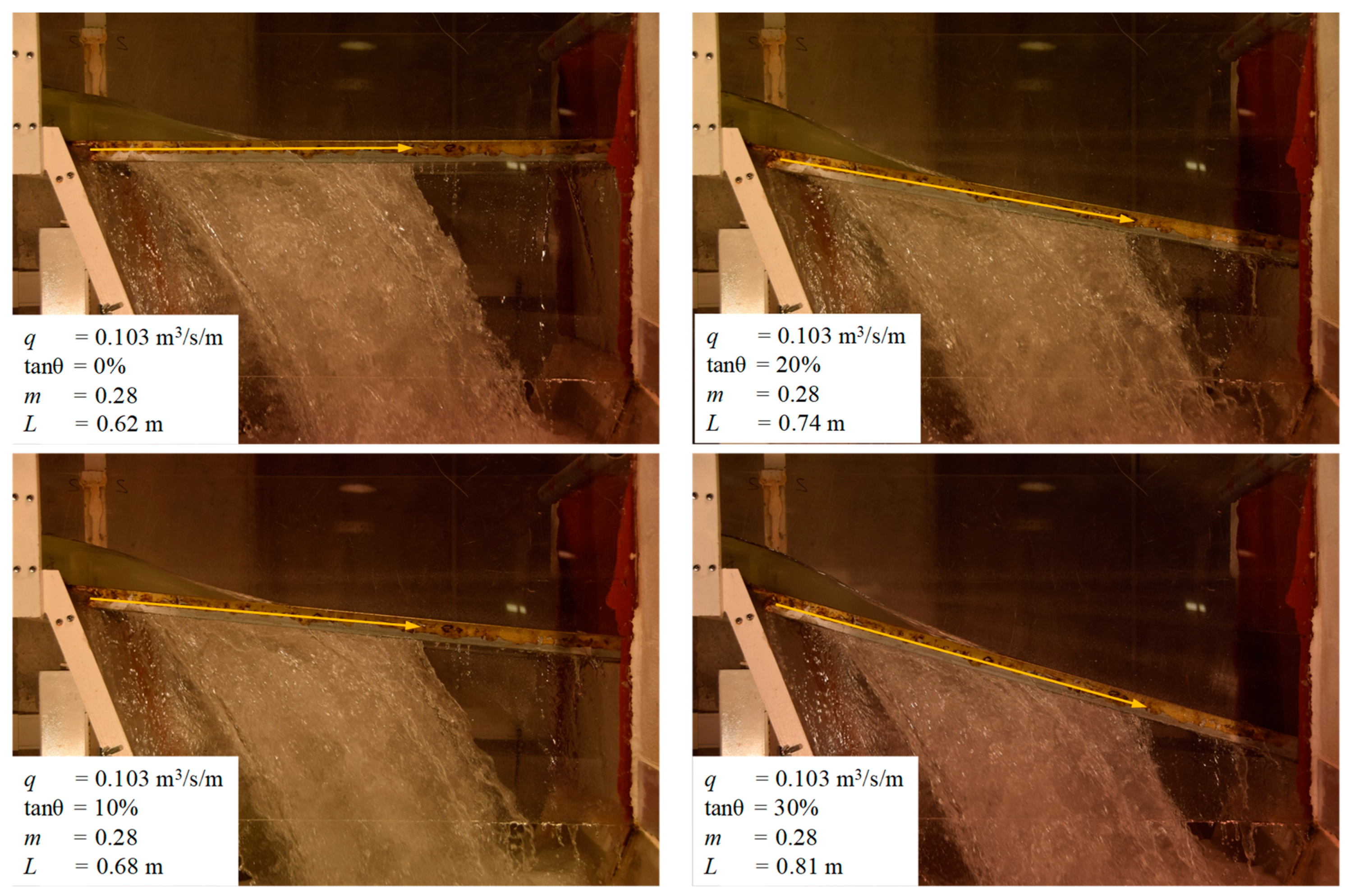
To extend Equation (4) to any void ratio and bar type, in the present work, the generalization of the values of the a, b, and C_q0 variables that appear in Equation (4), beyond the values presented in

Table 5. Constants of Equation (10) for the adjustment of the mean discharge coefficient $\overline{C_{qH}}$ [25].

Bar Type	m	a	b
T	0.16	3.3	0.05
T	0.22	2.1	0.05
T	0.28	1.5	0.05
O	0.28	1.45	0.05
O	0.60	0.70	0.20

were sought. The wetted rack length is defined as the maximum length reached by the flow over a rack to completely derive the incoming flow [20]. The total wetted length, L, can be observed in Figure 8, as the photos clearly show. These rack lengths must usually be measured experimentally in the laboratory.

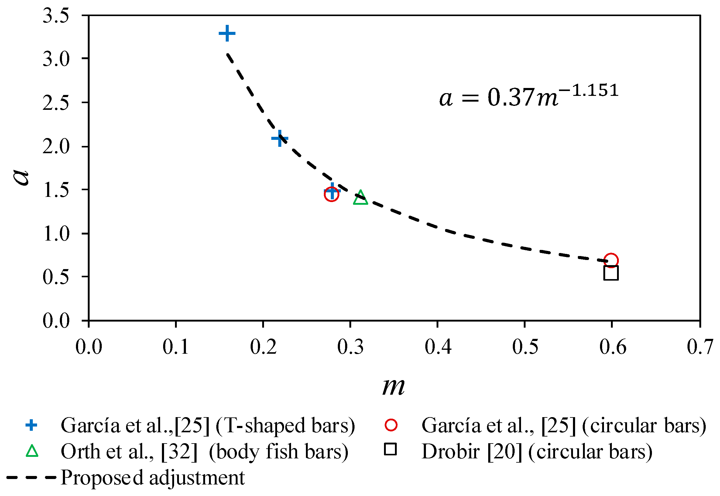
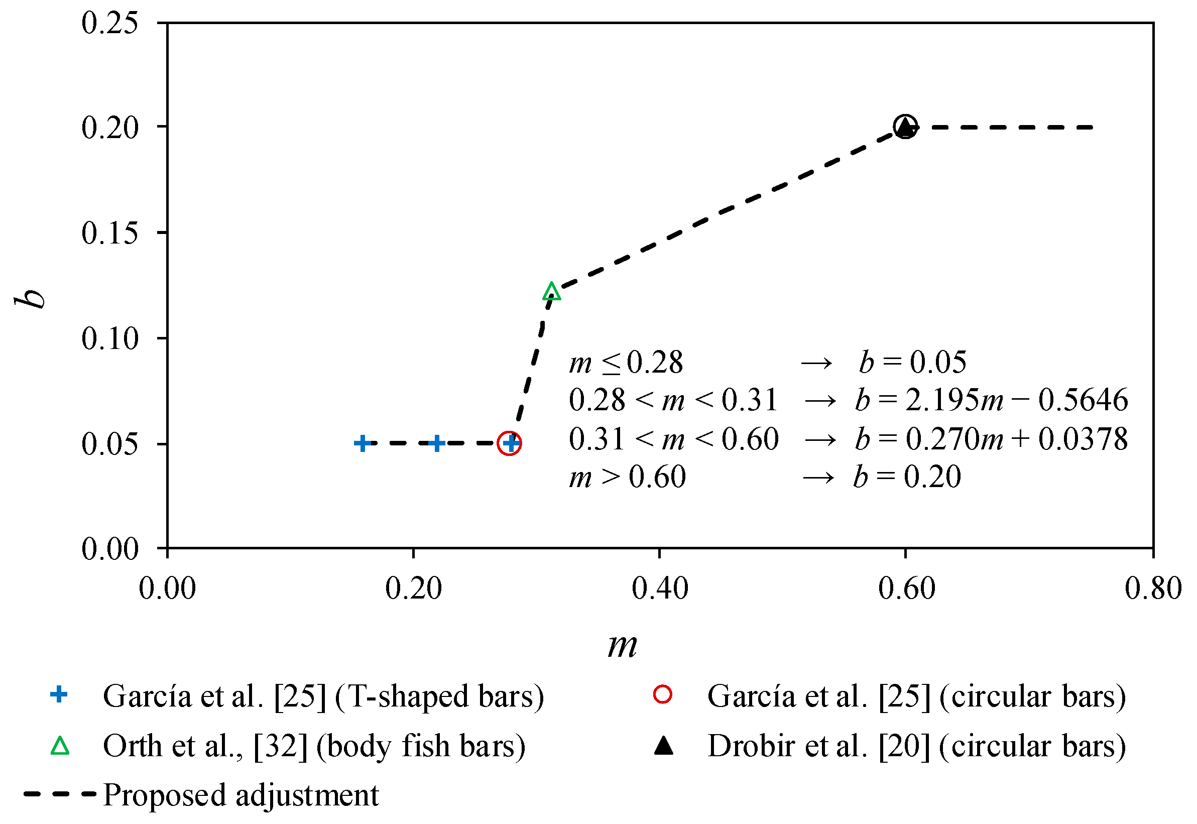
Figure 9 and Figure 10 present the proposed adjustments values of variables a and b, depending on the void ratio. Some of these values come from other experimental works [20,31]. The adjustments included in Figure 9 and Figure 10 enable the use of Equation (4) to be extended for the calculation of the mean discharge coefficient at any void ratio, m, bar type, and flow rate to derive. However, the present work focused on four types of bars, namely: T-shaped, circular, prismatic rounded, and fish body-like. In the case of Figure 10, more experimental tests are recommended in the future in the void ratio range 0.3–0.5 to improve this adjustment that is proposed as a linear transition between the known values.

The static discharge coefficient proposed by the authors from experimental measurements [22] is presented in Figure 11, including four different bar types: fish body, circular, prismatic top rounded, and T-shaped. The coefficients proposed by Frank [14,15] are included.

The equations associated with the adjustments proposed and the static discharge coefficients are presented below:

$$a=0.37m^{-1.15}$$

(8)

$$\begin{gathered} \mathrm{If} m \le 0.28 \to b=0.05 \\ \mathrm{If} 0.28<m<0.31 \to b=2.195m-0.5646 \\ \mathrm{If} 0.31\le m<0.60\to b=0.270m+0.0378 \end{gathered}$$

(9)

$$C_{q0}=c{e}^{-0.77m}$$

(10)

where c is a factor that depends on the shape of the bars: 1.52 for fish body bars, 1.43 for circular bars, 1.15 for prismatic rounded bars, and 0.90 for T-shaped bars. Once the previous parameters have been calculated, the rack length can be obtained as:

$$L=\frac{q}{\overline{C_{qH}}m\sqrt{2g{H}_{min}}},$$

(11)

where H_min = 1.50h_c, is the minimum energy of the flow and $\overline{C_{qH}}$ the mean discharge coefficient according to Equation (4). Equation (11), comes from the classical orifice equation $\frac{dq}{dx}=C_{qH}\left(x\right)m\sqrt{2g{H}_{min}}$. In this equation, x is the rack length longitudinal coordinate, H_min the energy height at the beginning of the rack that is the energy associated to the critical conditions, i.e., minimum energy, θ the angle between the bottom rack and the horizontal, m the void ratio, and g the gravitational acceleration. Once integrated along the wetted rack length considering a mean discharge coefficient, $\overline{C_{qH},}$ the Equation (11), is obtained. In equation (11), L is the wetted rack length. In the lab, L was measured for more than 376 different cases. Other cases proposed by [20,31] from field and lab experiments were also included to support the proposed Equations. Equation (10), presents the static discharge coefficient, C_q0, adjusted from experimental measurements. This was obtained in the lab disregarding the approaching velocity, placing a vertical wall at the end of the rack. Therefore, there is only potential energy and the Froude number of the approaching flow, F_r0, tends to 0. In the lab, the flow depth for different flowrates were measured and the orifice equation was solved, obtaining the static discharge coefficient. Results were in agreement with those proposed by several authors [7,10,11,14,15,17]. The Equation (10), was originally published in [16,22]. In the present work, new adaptations have been done to include the static discharge coefficient associated to other profiles like the fish body bars. Regarding Equations (8) and (9), from dimensional analysis, it was previously stated that $\overline{C_{qH}}=f\left(q^{power},tan\theta ,m,C_{q0}\right)$ [25]. In agreement with this, it was proposed that Equation (4),$\overline{C_{qH}}=\frac{am{C}_{q0}}{\left(1+tan\theta \right)}{q}^b$, which was also derived from the analysis of the experimental data. Equation (4) includes two variables, “a” and “b”. These parameters were proposed for the generalization of Equation (4) to any void ratio and are a novelty of the current work. The variable “a” takes into account the influence of the void ratio (in Figure 9, it follows a potential law); and the variable “b” accomplishes the potential law shown in the dimensional analysis, which relates $\overline{C_{qH}}$ and the specific discharge, q, for any void ratio. Both variables together with the static discharge coefficient allow for the extension of Equation (4) to any void ratio and bar profile.

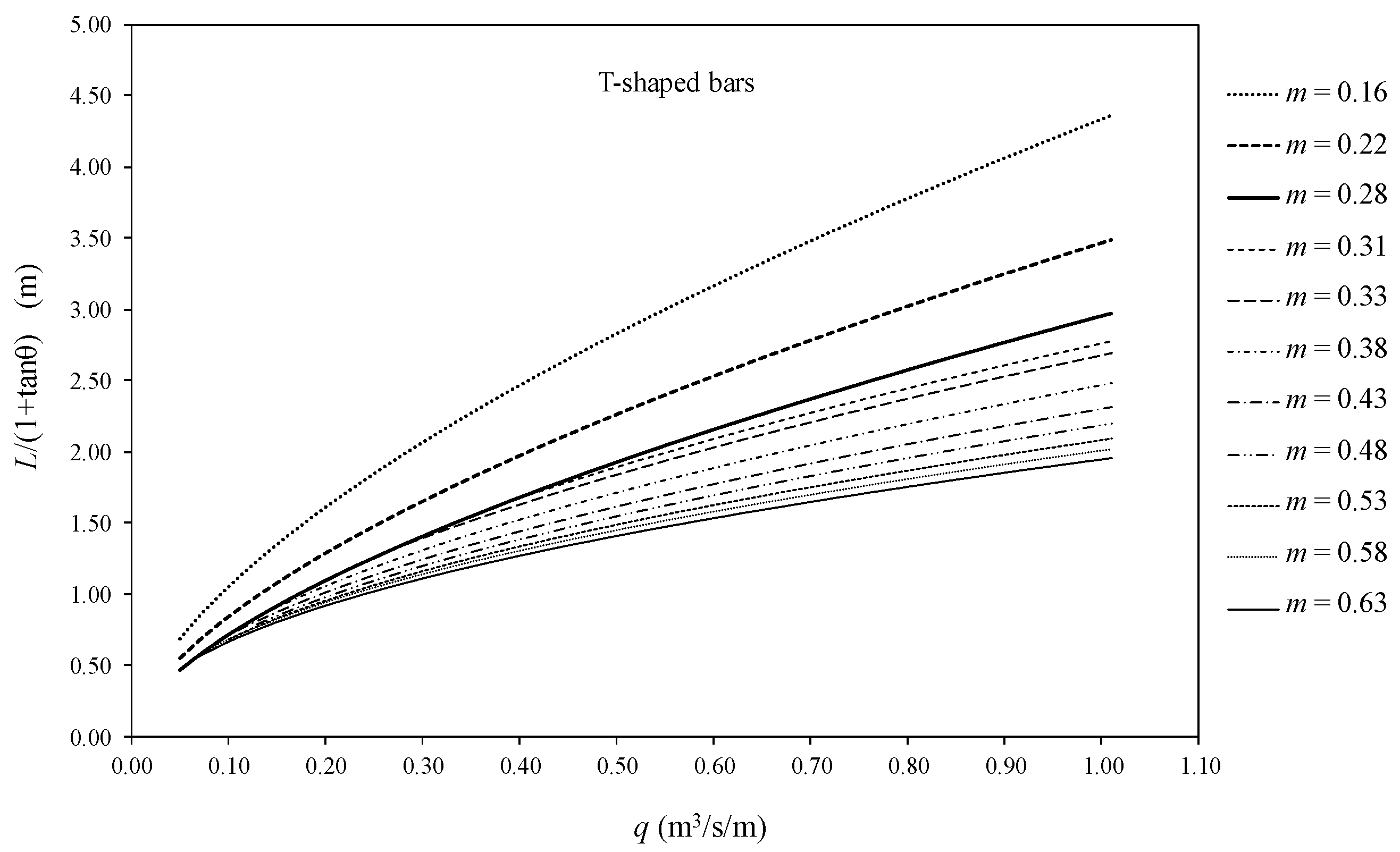
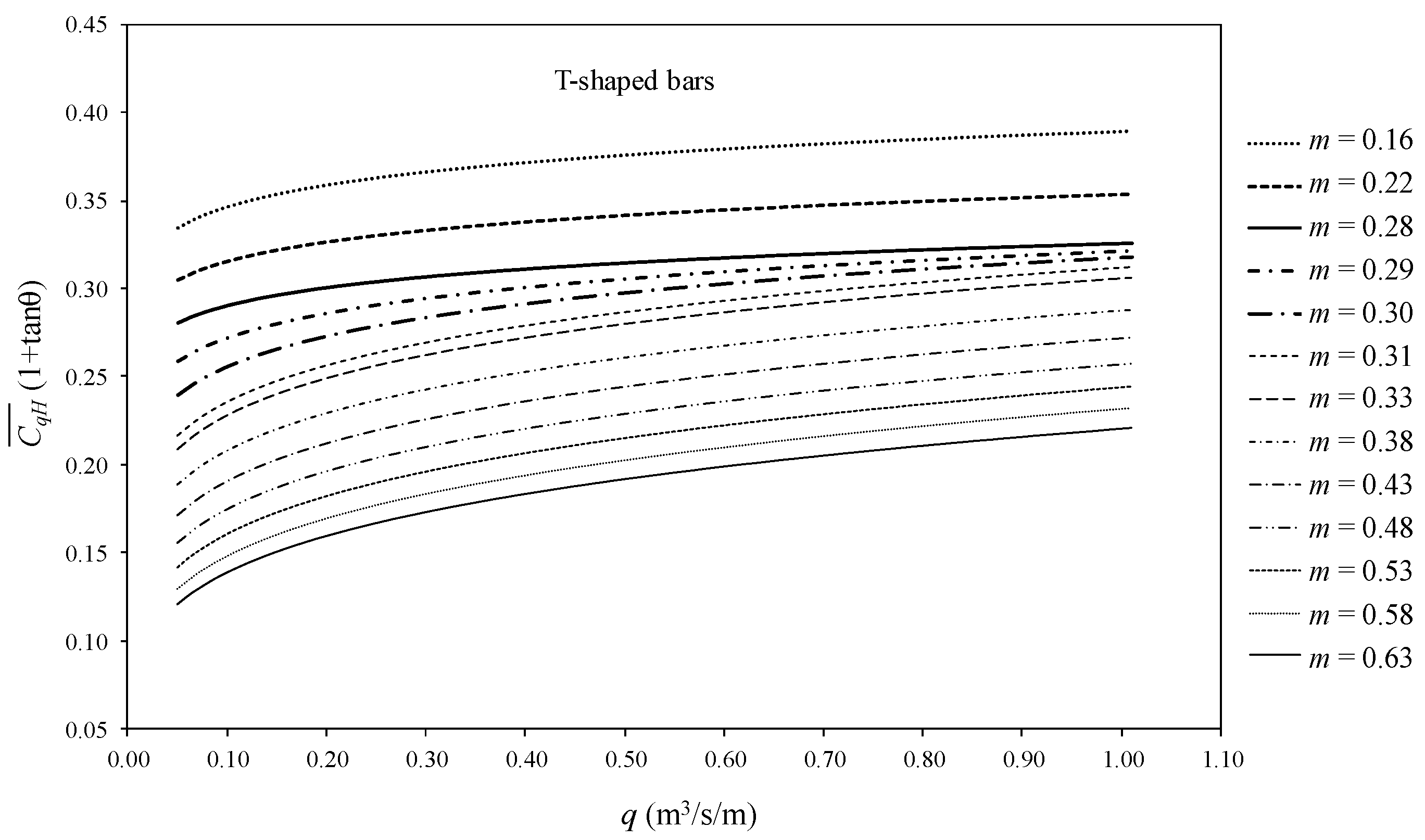
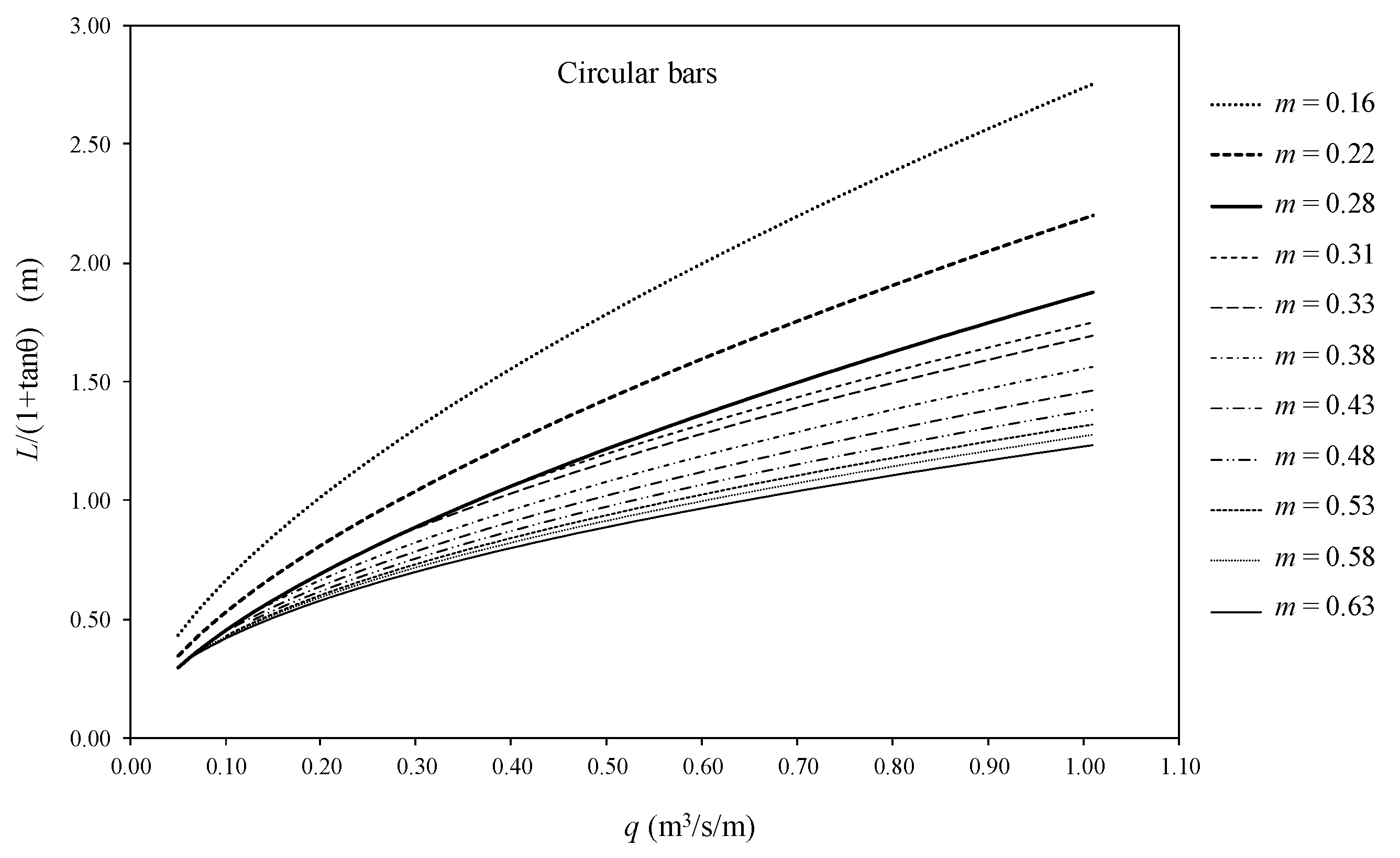
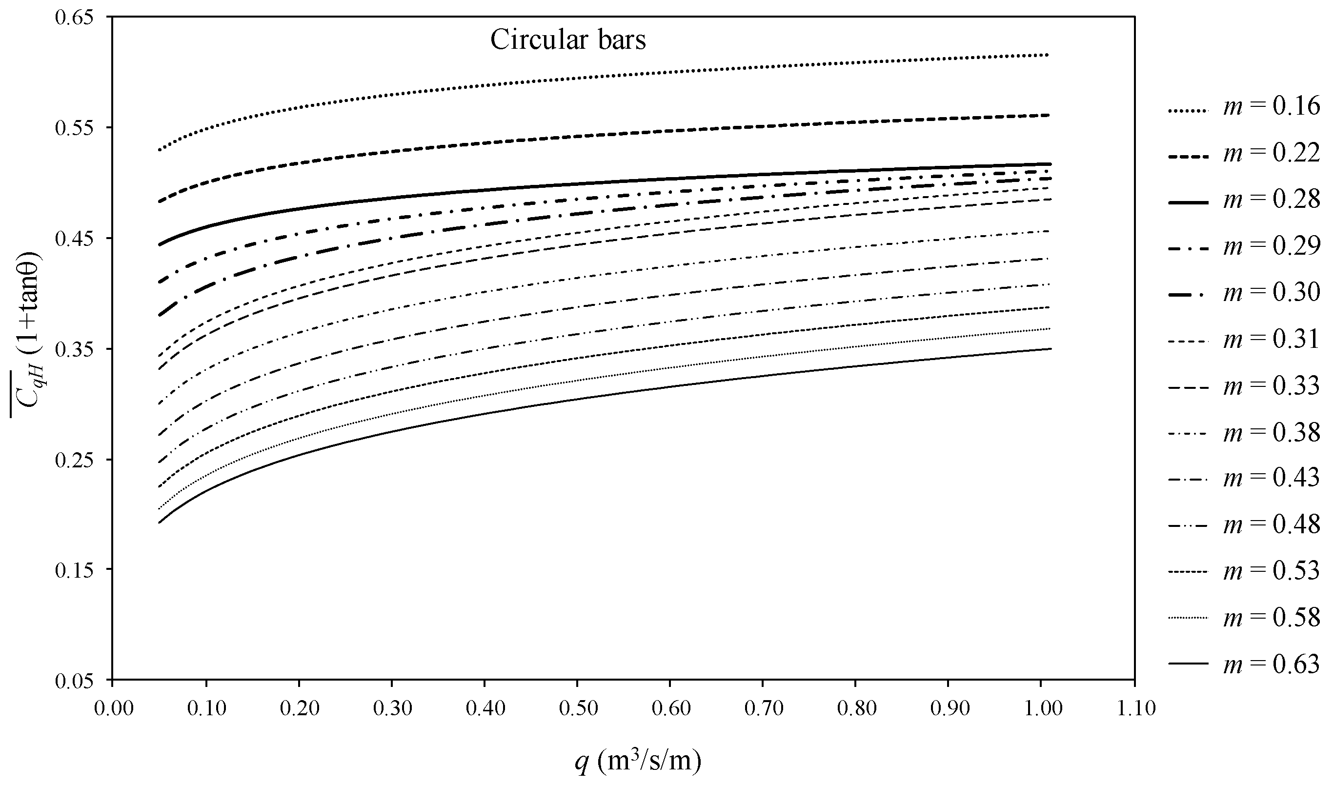
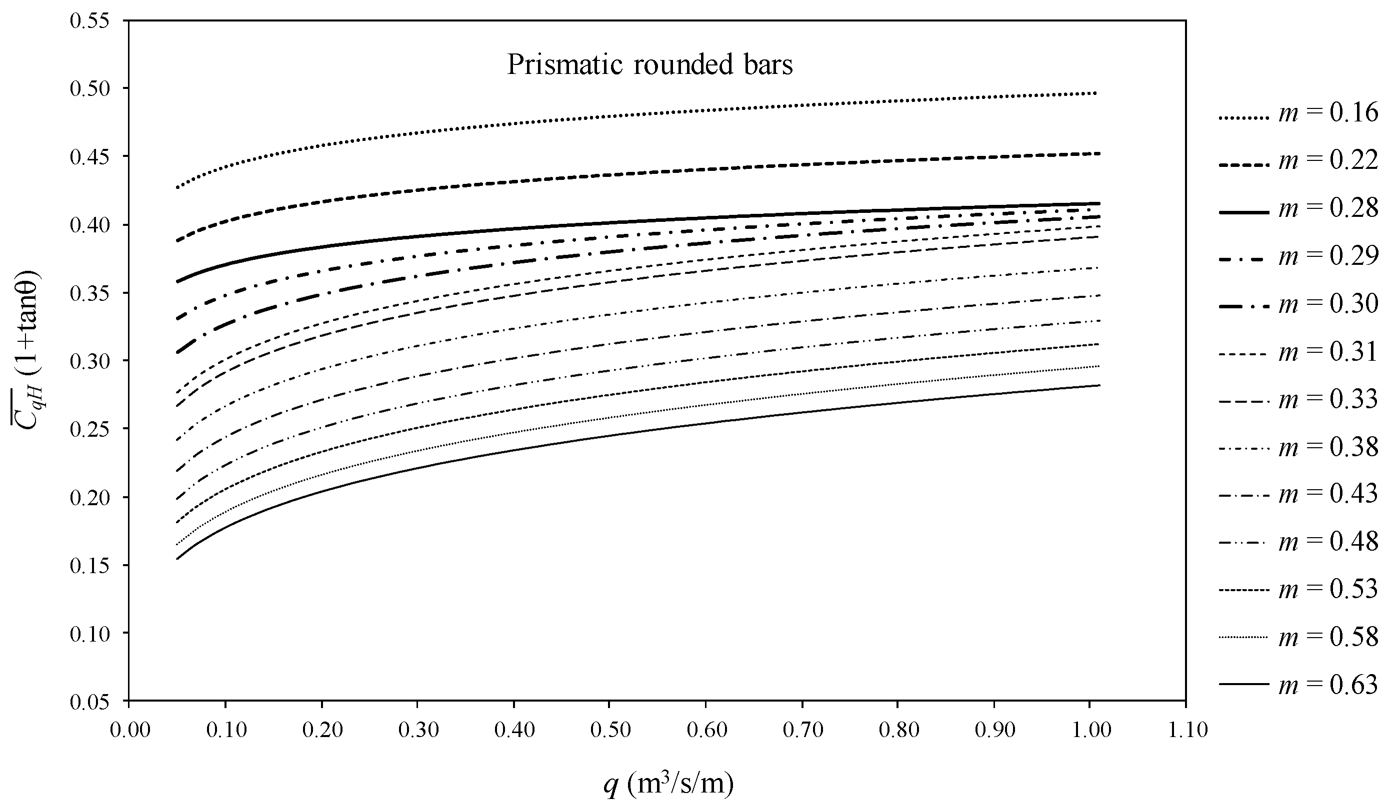
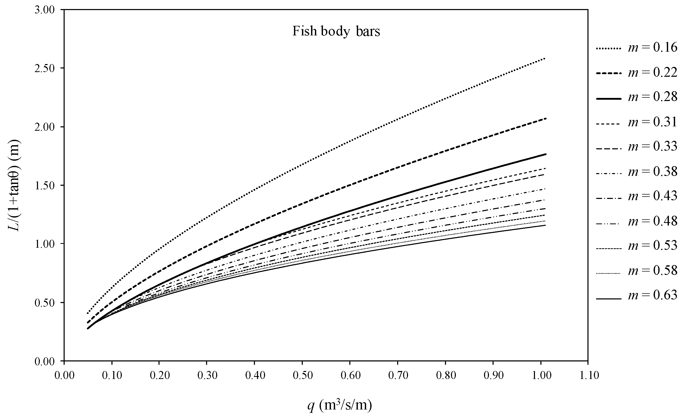
The extension of previous equations gives rise to a proposed series of designing nomograms. These are two dimensional diagrams that would allow the approximate graphical computation of the rack length. As commented, in the present work we included only four types of bars. Once the static discharge coefficient is known, the nomograms could be extended to any bar once the variables a and b are available from Figure 9 and Figure 10, and this serves for all the cases. Figure 12, Figure 13, Figure 14, Figure 15, Figure 16, Figure 17, Figure 18 and Figure 19 present the proposed nomograms in the case of the four different bar types. Factors of the length of the rack, L, and mean d discharge coefficient, $\overline{C_{qH}}$, for different slopes, void ratios, and longitudinal slopes are presented for the design of the bottom racks.

3.2. Occlusion Factor from Experiment Data

Research works about the effects of gravel size materials in the different configurations of the bottom racks have been extensively studied through more than 300 tests at the Universidad Politécnica de Cartagena [26,27,29,30], as described in Table 4. The occlusion factor is the factor that multiplies the wetted rack length calculated in clear water to the required length of the rack to derive a flow considering the occlusion phenomenon, $f=L_{\mathit{occlusion}}/L_{\mathit{clear}\mathit{water}}$. According to this percentage of efficiency in occlusion cases, it may be calculated by subtracting the unit from the occlusion factor. The tests that include gravels show scatter results in the occlusion factor. This is not considered as an error, but a deviation due to the stochastic nature of the phenomenon of the sediment transport and the different conditions of the experiments like longitudinal slope and flowrate. In lower flow rates, the percentage of clogging may increase considerably. The following figures include a summary of the results obtained in the different cases studied and from these, occlusion factors are proposed to be considered in the design. As presented in Table 4, racks with T-shaped bars were investigated with three different gravels: g₁ with d₅₀ = 8.3 mm, g₂ with d₅₀ = 14.8 mm, and g₃ with d₅₀ = 22.0 mm. The d₅₀ of the gravels is similar to the space between the bars, which favors the embedding of the gravels in the slits between the bars. The mean values of the occlusion factor f, obtained in the experimental campaign, can be observed in Figure 20. These values were in the range of 1.65–1.37 for longitudinal slopes of 0–33%, and the minimum mean occlusion factor achieved in the 30% slope was 1.35. The mean of the occlusion factors of T-shaped bars was calculated, omitting the higher value of f in each figure, under the consideration that this value would excessively penalize their design. From this, the deviation of each of the figures in terms of the occlusion factor was between 0.12 and 0.18.

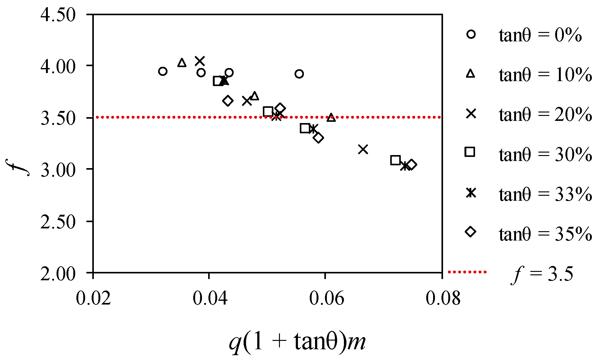
In the case of racks with circular bars, the void ratio m = 0.28 was investigated with gravel g₃ and d₅₀ = 22.0 mm. The results are presented in Figure 21.

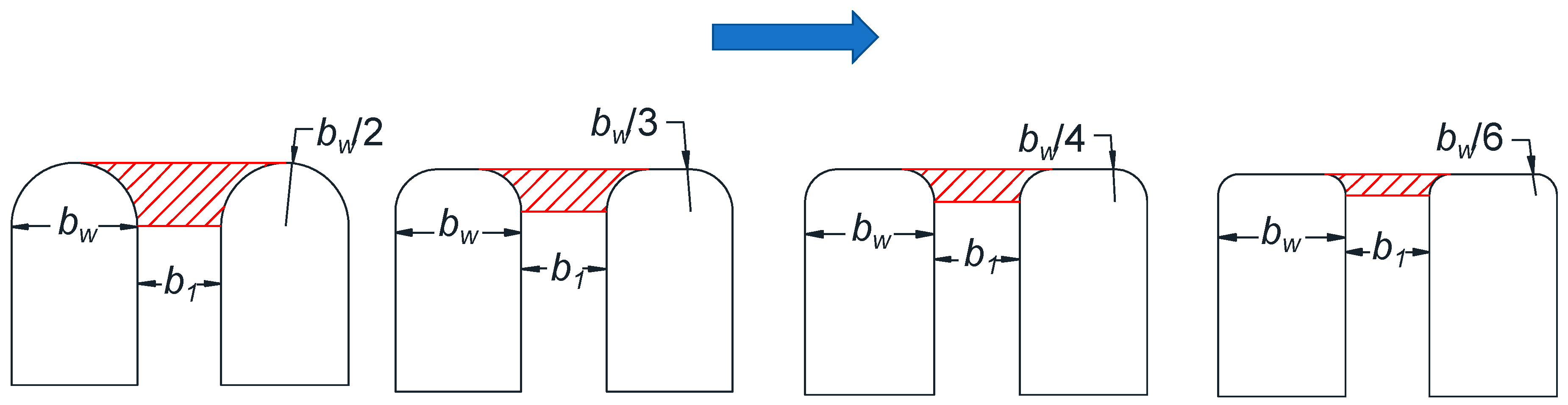
It can be observed that a high occlusion factor was obtained for the racks with circular bars, with the mean value being around 3.50. Experimentally measured occlusion factors yielded an important dispersion. In circular bars, the deviation achieved, in terms of the occlusion factor, was around 0.77. These racks are not recommended if occlusion due to gravels may occur [29]. To understand the influence of the shape of the profiles in the occlusion of the racks, Figure 22 is included. The red lines indicate the potential occlusion zone. In the case of profiles with a high radius, their area is higher and occlusion is favored to a broader range of diameters. In addition to a larger area, there is a greater contact length between the embedded gravels and the bar profile, which is also proportional to the drag force required to remove gravels embedded in the slit between two bars. Thus, profiles with a larger length and area of contact are more susceptible to having important occlusions factors. Figure 22 shows some cases in which, with the reduction of the radius of the top of the profiles, this effect can be reduced.

If we look in the bibliography, we can find the recommendations of previous authors, coming more from experiences in the maintenance than from experimental campaigns. For instance, Krochin [12] recommended the use of T-shaped or prismatic bars. The recommendations for the occlusion factor in the bibliography are: Krochin [12] f = 1.15–1.30; Drobir [13] and Simmler [19] f = 1.50–2.00; Andaroodi and Schleiss [2] and Lauterjung and Schmidt [18] f = 1.20; Bouvard [32] f = 1.50 to 2.00; Castillo et al. [26] and García [16] f = 1.30. Hence, the occlusion factor seems to be somewhere between 1.15 and 2.00 for T-shaped or prismatic bars. In circular bars, the occlusion factor may increase until f = 3.03 to 4.04 [29]. For this reason, circular bars are not recommended when occlusion phenomenon can occur.

3.3. Application Case

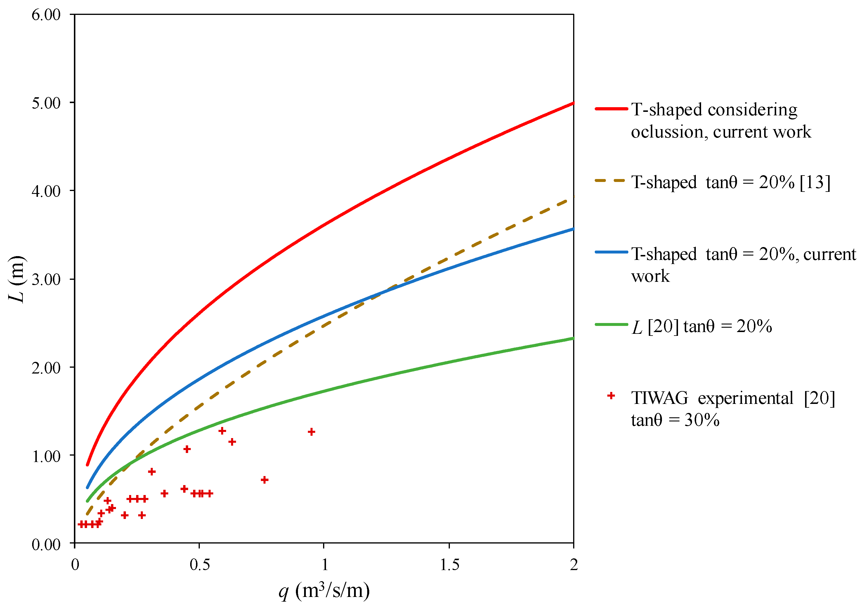
In this section, the wetted rack length proposed by previous researchers [13,20] was compared in the case of the void ratio, m = 0.60, circular bars, and slopes of 20% and 30%, which are the only cases available at prototype scale. Comparisons were also extended to values of the new methodology, including the occlusion factor. It can be observed in Figure 23 that the lengths are in agreement, in the case of considering T-shaped bars and an occlusion factor of 1.40, with the lengths proposed by [13] when considering double the wetted rack length. In the case of no occlusion, the lengths calculated with the new methodology coincide with those proposed by Drobir [20] (upper envelope at prototype scale).

3.4. Application to Design Cases in Ecuador

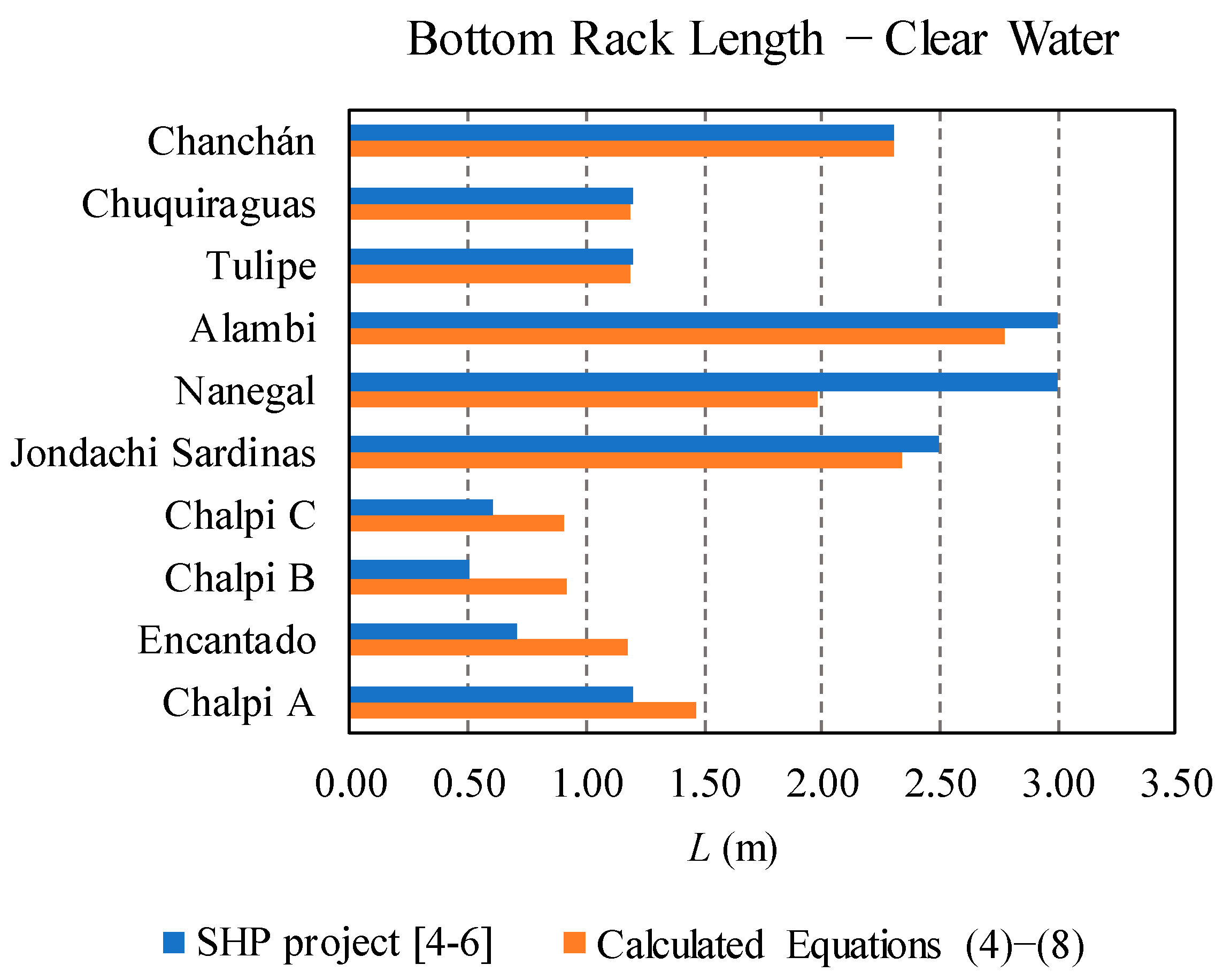
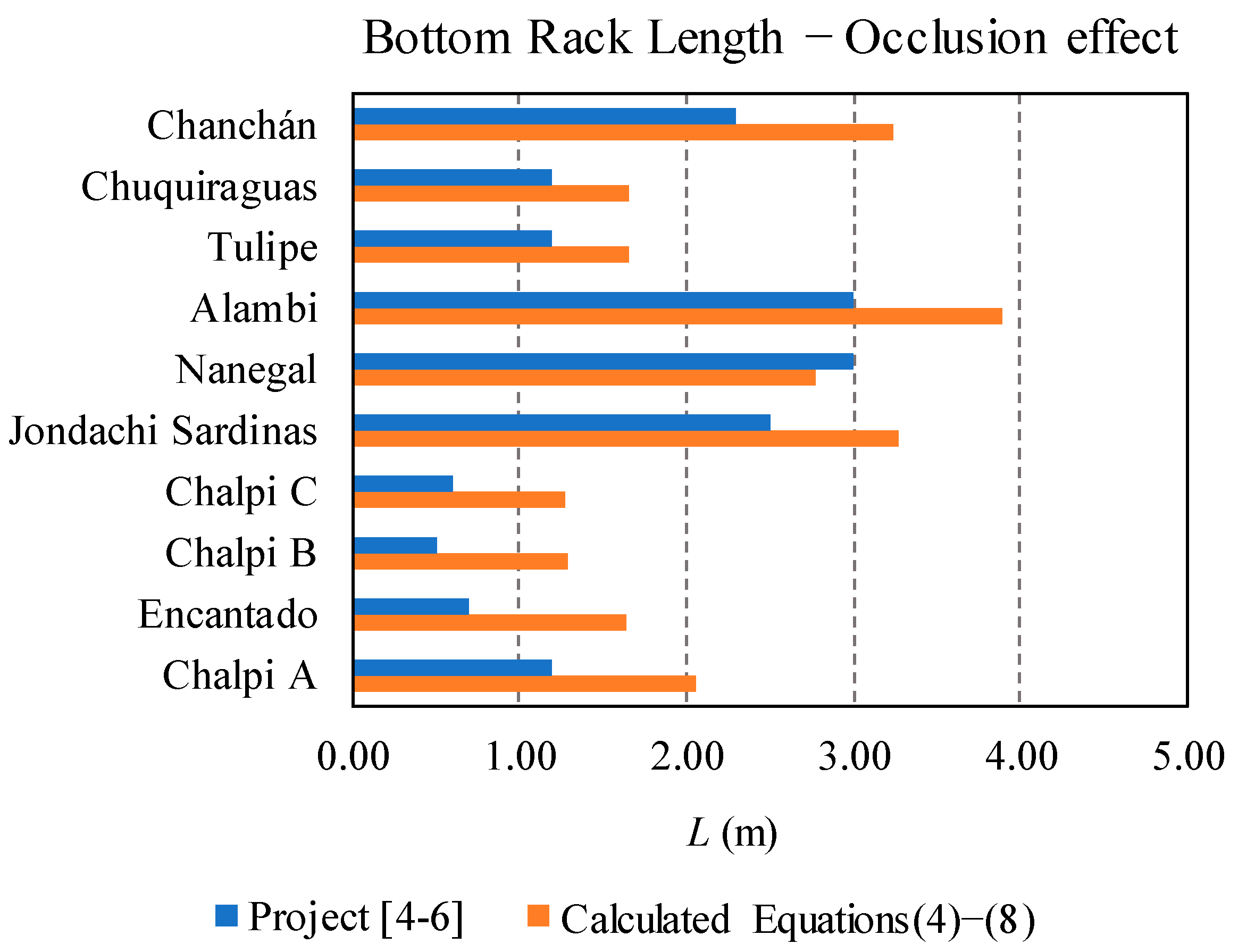
The information regarding the rack length included in the projects for the design of SHP in Ecuador [4,5,6] is included in

Table 6. Characteristics of the SHP projects in Ecuador [4,5,6]

Intake	Width of the River, Br (m)	Width of the Intake, B (m)	Design Flowrate, QD (m3/s)	Bar Type	Longitudinal Slope, tanθ (%)	b1 (m)	bw (m)	Void Ratio, m (-)	Rack Length, L
Chalpi A	35.00	6.00	2.20	T	20	0.050	0.030	0.625	1.20
Encantado	16.00	5.00	1.14	T	20	0.050	0.030	0.625	0.70
Chalpi B	12.00	3.50	0.47	T	20	0.050	0.030	0.625	0.50
Chalpi C	5.00	1.00	0.12	T	20	0.0254	0.020	0.559	0.60
Jondachi Sardinas	40.00	9.00	8.80	Prismatic	21	0.050	0.030	0.625	2.50
Nanegal	48.00	10.00	7.00	T	20	0.050	0.030	0.625	3.00
Alambi	17.00	8.00	11.50	T	20	0.050	0.030	0.625	3.00
Tulipe	6.00	6.00	1.40	T	20	0.050	0.030	0.625	1.20
Chuquiraguas	11.00	6.00	1.40	T	20	0.050	0.030	0.625	1.20
Chanchán	10.00	5.00	4.83	T	20	0.050	0.030	0.625	2.30

. This was compared with the values proposed by the methodology proposed in the present work through Equations (4)–(8) and with the occlusion factors proposed for T-shaped bars in Section 3.1. Figure 24, Figure 25 and Figure 26 present the comparison of both rack lengths, with and without the consideration of the occlusion factor.

The rack length proposed in the bottom intakes of the SHP in Ecuador [4,5,6] was calculated from the equations proposed by Frank (1)–(3), published in [13,14,15], using the static discharge coefficient, Cq₀, included in Figure 4, which was only for the void ratio of m = 0.60. Figure 24 shows that the rack lengths concur with those proposed by the present work.

In the case of changing the void ratio, the Frank formulation could not be applied. The equations proposed by [14,15] were also used to calculate the case of T-shaped rack lengths. These are compared in Figure 25 with that of the present work for the case of the longitudinal slope, tanθ = 20%. It can be observed how the differences between both lines increase with high and low flowrates, as both lines present different inclinations. The only exception presented is the Jondachi–Sardinas bottom rack design. In [4], it was reported that an increase of 20% in the minimum design length was considered to introduce the occlusion effect in the bottom rack grid with T-shaped bars. According to the experiments compiled in the current work, the occlusion factor recommends a 40% increase in the length.

The length of the racks proposed in the SHP design projects were compared with that of the present methodology, considering the occlusion factor proposed for the 20% slope (f = 1.40), in Figure 26. Important differences were observed. No increment due to occlusion was considered in the design of those intake systems.

3.5. Multi-Parametrical Tool for Designing Purposes

The computational tool created in Matlab^®, includes the methodology proposed in the current work and serves as a tool for the design of bottom racks with the possibility of taking into account multiple different parameters such as: clear water or with sediment dragging, different void ratios, bar types, longitudinal slope, and flowrates as presented below.

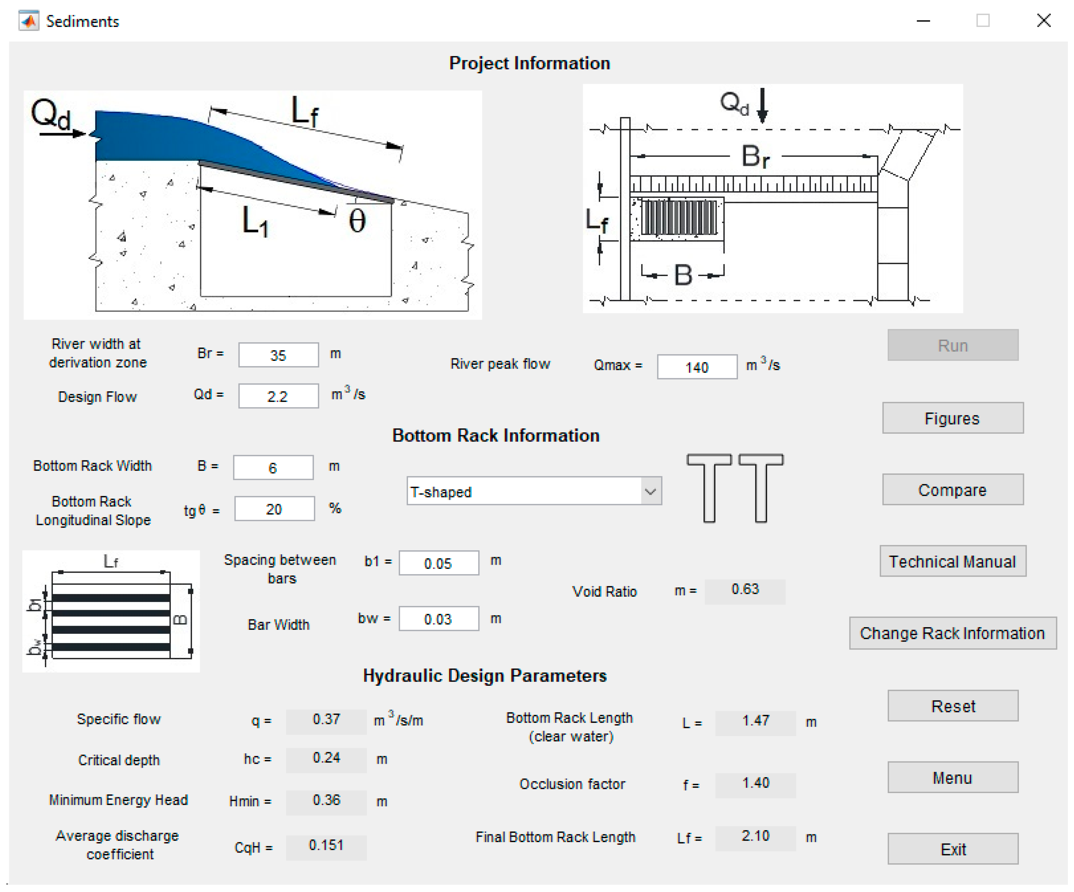
This computational tool is available online [33]. Figure 27 shows an image of the computational tool in which the following can be observed:

(a)

Project Information: This section is designed to enter information related to the design conditions of the bottom grid, such as the width of the section of the river where the intake will be located, B_r, and the design flow to derive, Q_d. Schemes of the components of the bottom intake are also included, as presented in Figure 27. This part also includes the bottom rack information, which allows the information chosen for the racks, such as rack width, B, longitudinal slope, tanθ, and the selection of bottom racks profile (fish body, T-shaped, and circular), to be entered. It also includes schemes of the selected rack profile and its components. The user also needs to provide the bar width, b_w, and bar spacing, b₁.

(b)

Hydraulic Design Parameters: This section presents the results of the calculations made by the program and the recommended rack length for the design. In the case of the design considering sediment clogging, the rack length is expressed as L_f, where f is the occlusion factor. The clear water design length is expressed by L.

Figure 27 shows the windows of the computational tool with the values of the Chalpi A bottom intake case study.

4. Conclusions

An extension of an existing methodology [25] is presented to calculate the required length of the rack in a bottom intake system, considering a broad range of bar profiles, void ratios, and slopes. This methodology improves the information in previous technical manuals [2,13,17,18,20], covering a broad range of bar profiles, void ratios, and flowrates. The present extended methodology is based on the experimental works carried out at the Universidad Politécnica de Cartagena from 2010 [16,21,22,23,24,25,26,27,28,29,30] and other experimental works both at prototype scale [20] and at laboratory scale [31]. The proposed extended methodology accomplishes the dimensional analysis of the discharge coefficient proposed in [25], where $\overline{C_{qH}}=f\left(q^{power},tan\theta ,m,C_{q0}\right).$

The Equations (4), (8), and (9) were validated with experimental data coming from: (1) circular bars with void ratio of 0.60 and 30% of longitudinal slope in a field prototype in the existing Tyrolean Weirs that belong to the power plant Sellrain-Silz (Tiroler Kraftwerke AG), carried out between 1988 and 1993; (2) fish body bar profile, with void ratio of 0.33, and longitudinal slope of 20%, for several flow rates, obtained by Orth [32] in a 1/5 scale model; (3) T-shaped and circular bars experiments with void ratios of 0.16, 0.22, 0.28, and 0.60; with flowrates from 0.05 to 0.2 m³/s/m and longitudinal slopes from 0 to 33% [25].

The proposed extended methodology generates a series of nomograms, or dimensional diagrams, to allow the approximate graphical computation of the required rack length. From this, the length of the rack can be selected from different settings of bar type. Four of those nomograms are presented in the current work (Figure 12, Figure 14, Figure 16 and Figure 18), for each of the four bar profiles presented. Their discharge coefficient can be also obtained from a series of proposed nomograms (Figure 13, Figure 15, Figure 17 and Figure 19).

The results of the extended methodology were compared with those proposed by Frank [14,15], Drobir [13,19], and Drobir [20] in Figure 23. It can be observed that the proposed methodology lengths are in agreement with those of Drobir [20], proposed as an envelope of the field campaign taken in a prototype for a void ratio m = 0.60. However, not the same agreement is observed with the previous methodologies [13,14,15,19]. The differences may come from the fact that those previous experiments were not considering the terms as the result of a dimensional analysis that could give rise to scale effects for high flow rates.

The consideration of the occlusion of the racks due to flow with gravel tests has been included. The occlusion factors are in the range of 1.65–1.37 for longitudinal slopes of 0–33%, in the case of T-shaped type bars. This factor grows to the range of three to four in the case of circular bars. These circular bar profiles are not recommended for occlusion cases. The current work highlights that occlusion effect increases in bar shapes with a larger area of contact, providing a suitable bed for the deposition of the materials. Finally, the comparison with ten existing SHP bottom intake designs in Ecuador [4,5,6] has also been studied and discussed in the present work. Good agreement is observed when the occlusion factor is not considered. However, these design lengths are lower than those recommended by this methodology in the case of occlusion effects.

A computational tool developed in Matlab, DIMRACK, which is available online [33], compiles all the conclusions of the current work and serves as a tool for the design of bottom racks. It allows users to consider multiple different parameters, such as different void ratios, bar types, longitudinal slope, and flowrates.

References

- CENACE. Available online: http://www.cenace.org.ec/ (accessed on 11 July 2019).
- Andaroodi, M.; Schleiss, A. Standardization of Civil Engineering Works of Small High-Head Hydropower Plants and Development of an Optimization Tool, LCH N 26: Communication; Laboratoire de Constructions Hydrauliques, Ecole Polytechnique Fédérale de Lausanne: Lausanne, Switzerland, 2006. [Google Scholar]
- Proyecto Mazar-Dudas. Available online: https://www.celec.gob.ec/hidroazogues/proyecto (accessed on 6 July 2018). (In Spanish).
- Andrade Borges, A.P.; Heredia Hidalgo, B.A. Diseño de Las Obras Hidráulicas de La Alternativa Técnica de La Central Hidroeléctrica Sardinas Grande, Provincia de Napo; Pontificia Universidad Católica del Ecuador: Quito, Ecuador, 2013. (In Spanish) [Google Scholar]
- Escuela Politécnica Nacional, (Facultad de Ingeniería Civil y Ambiental); Ministerio de Electricidad y Energía Renovable. Diseño a nivel de Prefactibilidad de Cinco Centrales Hidroeléctricas: Nanegal, Tulipe, Chuquiraguas, Huarhuallá y Chanchán; Ministerio de Electricidad y Energía Renovable: Quito, Ecuador, 2008. (In Spanish) [Google Scholar]
- ASTEC Cía. Ltda. Estudios de Factibilidad y Diseños Definitivos de la Primera Etapa del Proyecto de Agua Potable Ríos Orientales, Ramal Chalpi Grande—Papallacta; Empresa Pública Metropolitana de Agua Potable y Saneamiento: Quito, Ecuador, 2012; p. 74. (In Spanish) [Google Scholar]
- Righetti, M.; Lanzoni, S. Experimental Study of the Flow Field over Bottom Intake Racks. J. Hydraul. Eng. 2008, 134, 15–22. [Google Scholar] [CrossRef] [Green Version]
- Motskow, M. Sur le calcul des grilles de prise d’eau. La Houille Blanche 1957, 4, 569–576. (In French) [Google Scholar]
- Vargas, V. Tomas de fondo. In Proceedings of the XVIII Congreso Latinoamericano de Hidráulica, Oaxaca, Mexico, 18–21 September 1998. (In Spanish). [Google Scholar]
- Brunella, S.; Hager, W.; Minor, H. Hydraulics of Bottom Rack Intake. J. Hydraul. Eng. 2003, 129, 2–10. [Google Scholar] [CrossRef]
- Noseda, G. Correnti permanenti con portata progressivamente decrescente, defluenti su griglie di fondo. L’Energia Elettr. 1956, 33, 565–588. (In Italian) [Google Scholar]
- Krochin, S. Diseño Hidráulico, 2nd ed.; EPN: Quito, Ecuador, 1978; pp. 97–106. (In Spanish) [Google Scholar]
- Drobir, H. Entwurf von Wasserfassungen im Hochgebirge. Österreichische Wasserwirtsch. 1981, 11, 243–253. (In German) [Google Scholar]
- Frank, J.; Von Obering, E. Hydraulische Untersuchungen für das Tiroler Wehr. Bauingenieur 1956, 31, 96–101. (In German) [Google Scholar]
- Frank, J. Fortschritte in der hydraulic des Sohlenrechens. Bauingenieur 1959, 34, 12–18. (In German) [Google Scholar]
- García, J.T. Estudio Experimental y Numérico de Los Sistemas de Captación de Fondo. Ph.D. Thesis, Universidad Politécnica de Cartagena, Cartagena, Spain, June 2016. (In Spanish). [Google Scholar]
- Sotelo, G. Hidráulica de Canales; Facultad de Ingeniería Ediciones, Universidad Nacional Autónoma de México: Ciudad de México, México, 2002. (In Spanish) [Google Scholar]
- Lauterjung, H.; Schmidt, G. Planning of Water Intake Structures for Irrigation or Hydropower; A Publication of GTZ-Postharvest Project; Deutsche Gesellschaft für Technische Zusammenarbeit (GTZ) GmbH: Harare, Zimbabwe, 1989. (In German) [Google Scholar]
- Simmler, H. Konstruktiver Wasserbau; Technische Universität Graz, Institut für Wasserwirtschaft und konstruktiven Wasserbau: Graz, Austria, 1978. (In German) [Google Scholar]
- Drobir, H.; Kienberger, V.; Krouzecky, N. The wetted rack length of the Tyrolean Weir. In Proceedings of the IAHR-28th Congress, Graz, Austria, 22–27 August 1999. [Google Scholar]
- Castillo, L.G.; Lima, P. Análisis del dimensionamiento de la longitud de reja en una captación de fondo. In Proceedings of the XXIV Congreso Latinoamericano de Hidráulica, Punta del Este, Uruguay, 25 December 2010. (In Spanish). [Google Scholar]
- Castillo, L.G.; García, J.T.; Carrillo, J.M. Influence of rack slope and approaching conditions in bottom intake systems. Water 2017, 9, 65. [Google Scholar] [CrossRef]
- Carrillo, J.M.; Castillo, L.G.; García, J.T.; Sordo-Ward, A. Considerations for the design of bottom intake systems. J. Hydroinform. 2018, 20, 232–245. [Google Scholar] [CrossRef]
- Castillo, L.G.; García, J.T.; Haro, P.; Carrillo, J.M. Rack length in bottom intake systems. Int. J. Environ. Impacts 2018, 1, 279–287. [Google Scholar] [CrossRef]
- García, J.T.; Castillo, L.G.; Carrillo, J.M.; Haro, P.L. Empirical, dimensional and inspectional analysis in the design of bottom intake racks. Water 2018, 10, 1035. [Google Scholar] [CrossRef]
- Castillo, L.G.; García, J.T.; Carrillo, J.M. Experimental measurements of flow and sediment transport through bottom racks-influence of gravels sizes on the rack. In Proceedings of the International Conference on Fluvial Hydraulics, Lausanne, Switzerland, 3–5 September 2014; pp. 2165–2172. Available online: http://www.upct.es/hidrom/publicaciones/congresos/sizes_on_the_rack.pdf (accessed on 1 August 2018).
- Castillo, L.G.; García, J.T.; Carrillo, J.M. Experimental and numerical study of bottom rack occlusion by flow with gravel-sized sediment application to ephemeral streams in semi-arid regions. Water 2016, 8, 166. [Google Scholar] [CrossRef]
- Carrillo, J.M.; García, J.T.; Castillo, L.G. Experimental and Numerical Modelling of Bottom Intake Racks with Circular Bars. Water 2018, 10, 605. [Google Scholar] [CrossRef]
- García, J.T.; Castillo, L.G.; Haro, P.L.; Carrillo, J.M. Occlusion in Bottom Intakes with Circular Bars by Flow with Gravel-Sized Sediment. An Experimental Study. Water 2018, 10, 1699. [Google Scholar] [CrossRef]
- Haro, P.L.; Castillo, L.G.; García, J.T.; Carrillo, J.M. Experimental study of clogging in bottom intakes. Case of circular bars with high void ratios. In Proceedings of the Adapting River Management in an Era of Change, Madrid, Spain, 15 November 2018. [Google Scholar]
- Orth, J.; Chardonnet, E.; Meynardi, G. Étude de grilles pour prises d’eau du type en-dessous. La Houille Blanche 1954, 9, 343–351. (In French) [Google Scholar] [CrossRef]
- Bouvard, M. Mobile Barrages & Intakes on Sediment Transporting Rivers; International Association of Hydraulic Engineering and Research (IAHR) Monograph: Rotterdam, The Netherlands, 1992. [Google Scholar]
- Haro, P.L.; García, J.T.; Castillo, L.G.; Carrillo, J.M. Dimrack, Matlab Central File Exchange 2019. Available online: https://www.mathworks.com/matlabcentral/fileexchange/72361-dimrack (accessed on 30 September 2019).
Figure 1.
View of the Chalpi A project: (a) construction of the first bottom intake system and sand trap; (b) detail of the bottom rack bar profile [6]; and (c) project location in Ecuador (without scale).
Figure 2.
Mazar Dudas Project: (a) Dudas bottom intake system [3]; (b) San Antonio bottom intake system [3]; and (c) project location in Ecuador (without scale).
Figure 3.
Scheme of the configuration of longitudinal racks in a bottom intake system.
Figure 4.
Rack length depending on the flowrate to derive, q, in case of m = 0.60 and longitudinal rack slope = 20% [7,8,9,10,11,12].
Figure 6.
Rack length depending on the flowrate to derive, q, in the case of m = 0.60 and longitudinal rack slope = 20% and 30%.
Figure 7.
Scheme of the intake system physical device at Universidad Politécnica de Cartagena.
Figure 8.
Wetted rack length for different flows and longitudinal slopes with racks made of circular bars and void ratio m = 0.28.
Figure 9.
Adjustment proposed for variable a according to experimental measurements.
Figure 10.
Adjustment proposed for variable b according to experimental measurements.
Figure 11.
Static discharge coefficient for different bar-types.
Figure 12.
Factor of wetted rack length in Equation (8), L, in the case of T-shaped bars for different void ratios, m, and flowrates, q.
Figure 13.
Factor of mean discharge coefficient in Equation (4), , for T-shaped bars depending on the void ratio, m, and the flowrate, q.
Figure 14.
Factor of wetted rack length in Equation (8), L, in the case of circular bars for different void ratios, m, and flowrates, q.
Figure 15.
Factor of mean discharge coefficient in Equation (4), , for circular bars depending on the void ratio, m, and the flowrate, q.
Figure 16.
Factor of wetted rack length in Equation (8), L, in the case of prismatic rounded bars for different void ratios, m, and flowrates, q.
Figure 17.
Factor of mean discharge coefficient in Equation (4), , for prismatic rounded bars depending on the void ratio, m, and the flowrate, q.
Figure 18.
Factor of wetted rack length in Equation (8), L, in the case of fish body bars for different void ratios, m, and flowrates, q.
Figure 19.
Factor of mean discharge coefficient in Equation (4), , for fish body bars depending on the void ratio, m, and the flowrate, q.
Figure 20.
Mean occlusion factor in the case of T-shaped bars.
Figure 21.
Mean occlusion factor in the case of circular bars with m = 0.28.
Figure 22.
View of the area and length of contact.
Figure 23.
Rack length depending on the flowrate to derive, q, in the case of m = 0.60 and longitudinal rack slope = 20%.
Figure 24.
Rack lengths calculated for SHP bottom intakes in Ecuador compared with the values proposed in the present work (clear water case).
Figure 25.
Rack length depending on the flowrate to derive, q, in the case of m = 0.60 and longitudinal rack slope = 20% according to Ecuador SHP designs, including the results of the current work.
Figure 26.
Rack lengths calculated for SHP bottom intakes in Ecuador compared with the values proposed in the present work, considering the occlusion factor f = 1.40.
Figure 27.
Window of the computational tool including the values of the Chalpi A case of study.