Characterisation of the Water Renewal in a Macro-Tidal Marina Using Several Transport Timescales


LIENSs, La Rochelle University, 2 rue Olympe de Gouges, 17000 la Rochelle, France
*
Author to whom correspondence should be addressed.
Water 2019, 11(10), 2050; https://doi.org/10.3390/w11102050
Submission received: 11 June 2019
/
Revised: 24 September 2019
/
Accepted: 26 September 2019
/
Published: 30 September 2019
(This article belongs to the Special Issue Tracer and Timescale Methods for Passive and Reactive Transport in Fluid Flows)
Abstract
:In this paper, we investigate the water renewal of a highly populated marina, located in the south-west of France, and subjected to a macro-tidal regime. With the use of a 3D-numerical model (TELEMAC-3D), three water transport timescales were studied and compared to provide a fully detailed description of the physical processes occurring in the marina. Integrated Flushing times (IFT) were computed through a Eulerian way while a Lagrangian method allowed to estimate Residence Times (RT) and Exposure Times (ET). From these timescales, the return-flow (the fraction of water that re-enters the marina at flood after leaving the domain at ebb) was quantified via the Return-flow Factor (RFF) and the Return Coefficient (RC) parameters. The intrinsic information contained in these parameters is thoroughly analysed, and their relevance is discussed. A wide range of weather-marine conditions was tested to provide the most exhaustive information about the processes occurring in the marina. The results highlight the significant influence of the tide and the wind as well as the smaller influence of the Floating Structures (FS) on the renewal. Besides, this study provides the first investigation of the water exchange processes of La Rochelle marina. It offers some content that interest researchers and environmental managers in the monitoring of pollutants as well as biological/ecological applications.
1. Introduction
Over the years, the increasing development of coastal areas has modified the quality of water and sediments as well as marine habitats. Ports, which are the main interfaces between cities and the sea, are primarily subjected to a multi-source of contamination due to intense anthropogenic activities. Their complex geometry and infrastructure (e.g., quays, channels, and docks) induce low circulation and stagnant waters which tend to enhance and to control the fate of contaminants. Given the tendency of pollutants to remain confined and settle on the bottom, the pollution generated within the ports is of grave concern. Then, improving water and sediment quality is of vital importance for the sustainable development of coastal waters.
In recent decades, managers have been under increasing pressure to demonstrate the environmental skills of the port they manage. Some studies focused on the effect of diffuse pollution originating from urban water runoffs and boat repair activities [1,2] as well as accidental oil spills [3,4]. Metal concentrations in water and sediments were also monitored and investigated [5,6] but characterising the water quality of such areas is still a challenge as it requires many parameters.
Although ports are considered as low-energy systems, the hydrological pattern established within the port basin cannot be neglected in any study [7]. The rate of renewal of a basin is useful information that provides a first-order description of its dynamics. Numerous transport timescales have been defined through the literature to quantify this renewal [8,9,10,11,12]. With the growing use of numerical modelling, these water transport timescales are useful parameters to condense the considerable amount of data in intelligible and quantitative information [13]. The most commonly used, “flushing time”, “residence time”, ”age”, and ”exposure time” have been applied in a wide range of studies all over the world [14,15,16,17]. From the environmental port management point of view, these transport timescales offer an interesting indication of the spatial and temporal variability of the dynamic and of the susceptibility to pollution. However, such timescale descriptors need to be carefully employed because there is no real consensus on their application [11].
After an expansion in 2014 (corresponding to the NE basin in Figure 1), La Rochelle Marina, located in the southwestern part of France, is currently considered as the biggest marina on the European Atlantic coast. Despite the environmental policy and ecological awareness of the marina, equipment and maritime activities may be a source of the pollution [18]. The main objective of this study is, therefore, to characterise the water renewal of La Rochelle Marina due to the horizontal and vertical variability of its currents. This contribution can be considered as a first scientific investigation because, even if the importance of such timescales is evident, no references or estimates were available in the literature for a similar marina.
To describe water renewal mechanisms accurately, we performed a large number of simulations with a 3D hydrodynamic model calibrated and validated in a previous study [19]. The specificity of the model is to take into consideration the considerable number of structures floating in the marina (e.g., docks, boats). In this study, three timescales are compared (flushing time, residence time and exposure time) to find the most relevant parameter to describe water renewal of the domain. Besides, we estimated the return-flow in different ways, the fraction of water that leaves the marina at ebb tide before re-entering it at the next flood tide [20], and its effect on the tidal flushing of the marina was analysed. The above-mentioned timescales and quantities were computed for different scenarios to characterise the influence of wind, tide and floating structures on the water renewal. In the next section, study site and numerical computations will be presented before introducing definitions and concepts of chosen timescales and quantities. In Section 3, a Lagrangian validation is carried out while timescale results are shown in Section 4 and discussed in Section 5.
2. Materials and Methods
2.1. Study Site
2.1.1. La Rochelle Marina
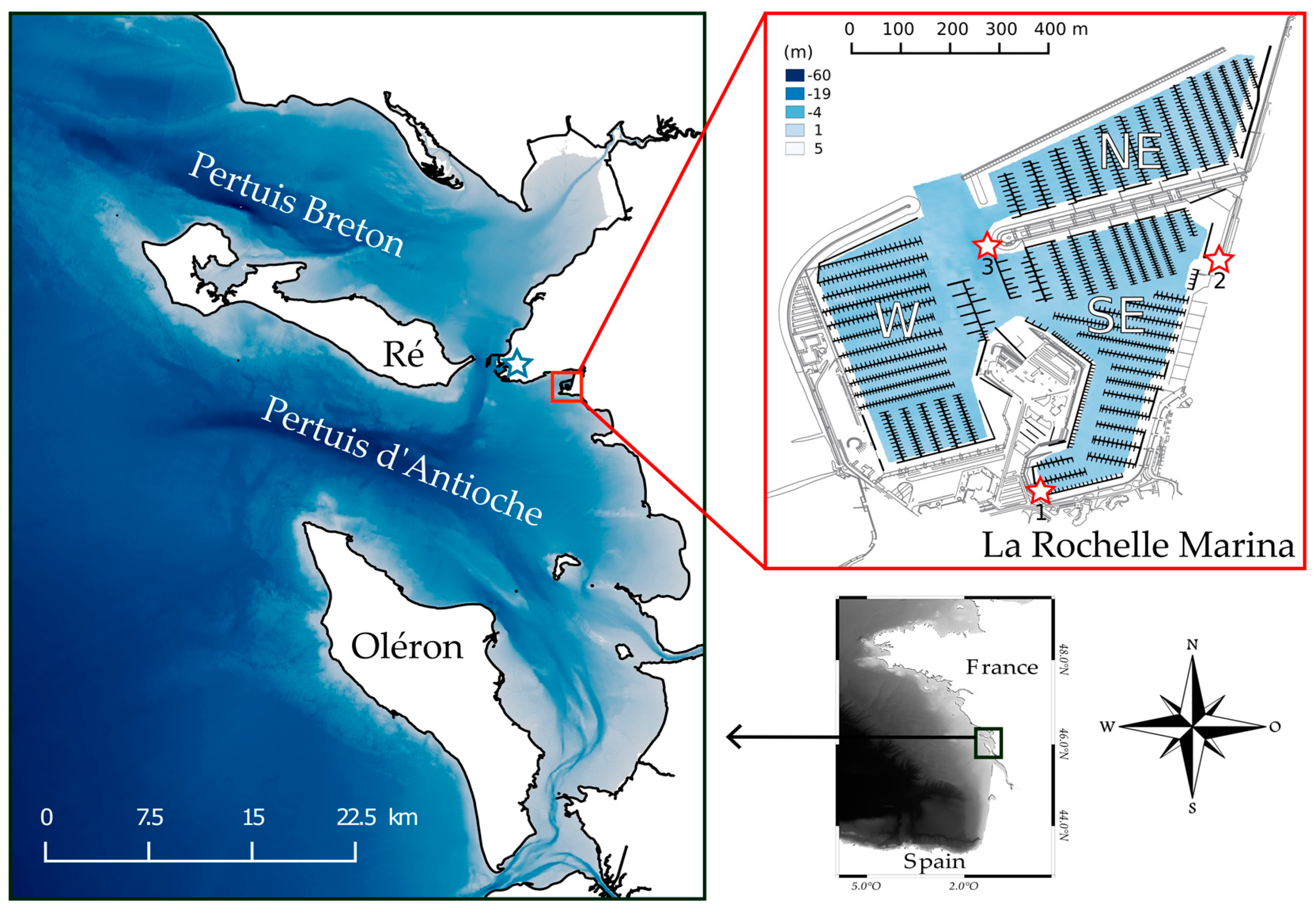
The city of La Rochelle, the provincial administrative centre of the department, has a land area of 28.43 km2 and a population of 80,000 inhabitants. Its marina, created in 1972, has been the biggest marina (50 ha) along the Atlantic coast, since its expansion in 2014. This 900 m-long and 820 m-wide semi-enclosed area is divided in three basins totalling 4500 moorings, distributed along 15 km of floating docks. The southeastern (SE) basin is the more prominent, with 22 ha, while the western (W) and the northeastern (NE) basin, present respectively 17 and 15 ha. At sea, the marina is accessible by a 110 m wide main entrance, while the NE basin offers two openings: 150 m wide to the northeast and a 64 m wide to the southwest which connects the NE basin to the W basin (Figure 1). The marina is not spared by siltation and has to spend 10 per cent of its total budget to dredge around 200 000 m3 of cohesive sediment each year. The annual sediment deposition can overpass 50 cm in some of its basins (Pers. Comm. La Rochelle Marina), which requires recurring dredging of the basins, 8 months a year.
The environmental policy of the marina led to an ISO 14001 certification, an international reference in sustainable development. Despite their effort, water quality and marine biodiversity are still impacted by intensive anthropogenic inputs. Several potential sources of contamination have been identified in the marina (symbolized in Figure 1): the rainwater outlet, where runoff waters from streets and roadways can flow abundantly during storm events; the fairing area where boats are maintained (antifouled, painted and sanded); the fuel station where dripping fuel can be discharged. We can also consider diffuse pollution from boat activities.
2.1.2. Geomorphology and Hydrodynamics of the Coastal Area
La Rochelle Marina is located in the northern landward part of the Pertuis d’Antioche embayment along the French Atlantic Coast, in the central part of the Bay of Biscay. This shallow water coastal area is protected from the Atlantic Ocean by Ré and Oléron islands and connected to the Pertuis Breton embayment through a narrow inlet. The bathymetry is characterised by silty to sandy-silty bottoms, with a 44 m deep trench and many tidal flats. The coastal area is considered as a mixed, wave and tide-dominated estuary [21]. The tidal regime is semidiurnal and tidal range varies from 2 m during neap tides to more than 6 m during spring tides. This macro-tidal environment is dominated by M2, and its amplitude grows to more than 1.8 m in the inner part of the estuaries due to resonance and shoaling [22]. Because of resonance occurring on the Bay of Biscay shelf, the quarter-diurnal tidal constituents (M4, MS4 and MN4) are strongly amplified shoreward [23]. In the embayments, average freshwater inflows are about 2 orders of magnitude less than tidal flows [24].
2.1.3. Meteorological Context
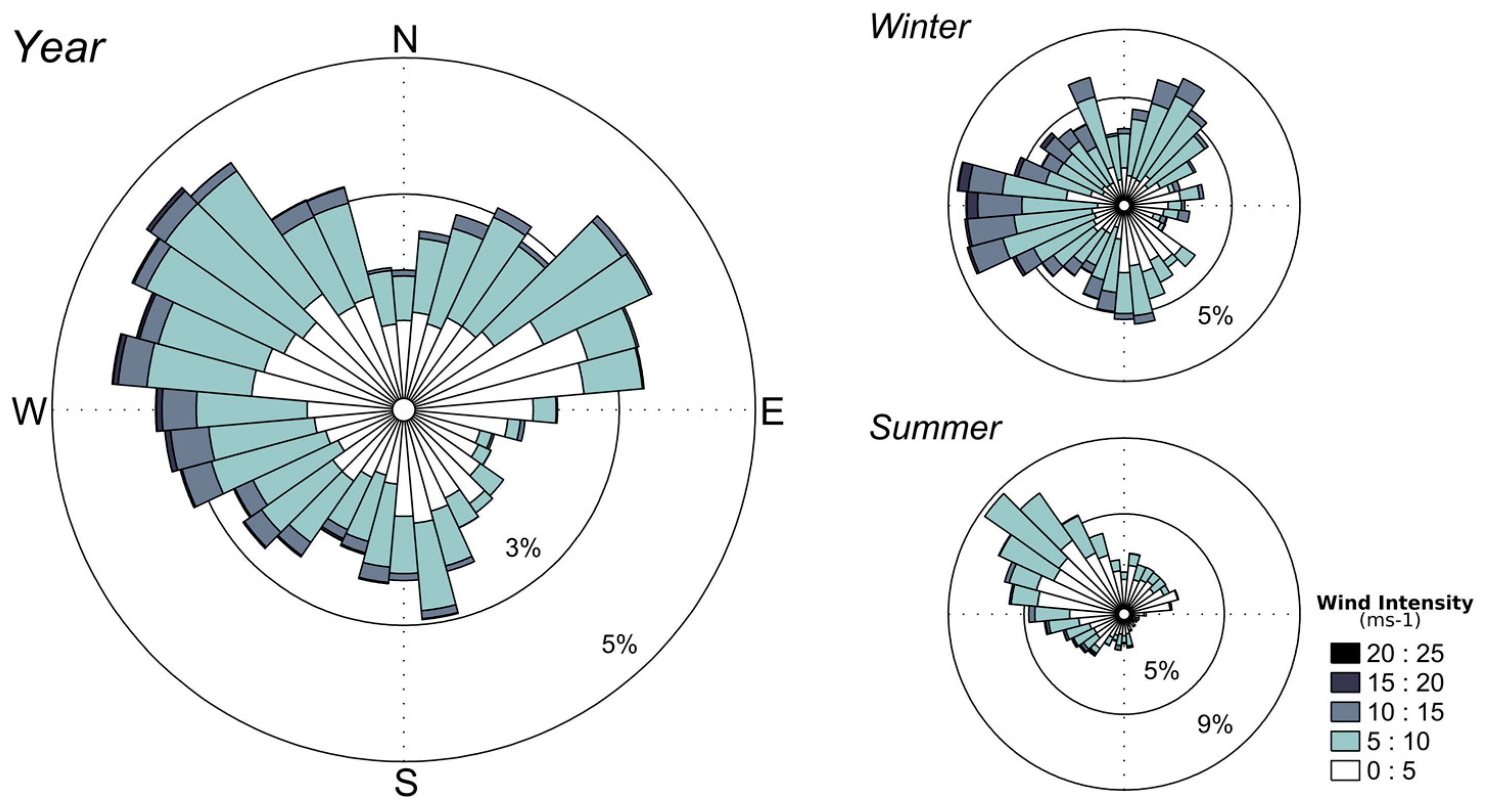
The study area is subjected to seasonal climate variations. Summer presents a weak low-pressure system activity resulting in weak northeasterly winds while northwest thermic breezes mainly dominate littoral. Low-pressure systems that cross the Atlantic Ocean from autumn are the most active during winter, generating extreme west and northwest winds. North Atlantic Oscillation (NAO) partly controls the inter-annual variability of the wind regime in the whole Bay of Biscay [25]. Weather-marine conditions were collected by La Pallice weather station (blue-bordered white star in Figure 1) over the temporal interval 2015–2018 (Figure 2). Data analysis reveals a predominance of four winds over the area of study: north-western (22% mean yearly occurrence), western (21% mean yearly occurrence), north-eastern (19% mean yearly occurrence) and southern (14% mean yearly occurrence).
2.2. Numerical Model Implementation
To calculate water transport timescales, we used the TELEMAC-3D model [26], a three-dimensional hydrodynamic model adapted to free-surface flow. In this study, three-dimensional Navier-Stokes equations were solved in non-hydrostatic mode. Bottom stress was computed through a Chézy parametrisation over an unstructured grid. The semi-implicit Galerkin finite element method is used to solve continuity and momentum equations and a Lagrangian-Eulerian treatment of advective terms and a semi-implicit way ensure numerical stability. More insight and details about the equations are presented in [19]. TELEMAC-3D provides the possibility of taking into account passive tracers in the model domain. The model solves the advection and diffusion equation of a conservative tracer.
The modelled area is 35 km wide and 100 km long and is discretised on a 41,000 nodes unstructured grid, with resolution from 2 km offshore to nearly 5 m in the marina [19]. The size of the computational domain (4757.9 km2) is considered sufficiently large so that the prescribed boundary conditions negligibly affect the tracer mass in the marina (0.5 km2) as requested by [27]. The model has eight vertical sigma levels, which are treated with the Arbitrary Lagrangian-Eulerian method [28] and lead to a total of 320,000 nodes. Our bathymetry originates from French Navy (hereafter SHOM) [29] and single beam surveys acquired in the marina. Then, the topography of intertidal areas is determined using a LiDAR survey, acquired in 2010 (LITTO3D, French National Geographic Institute and SHOM). Along its open boundary, the model is forced by 34 astronomical tidal constituents obtained by linear interpolation from the global tide model FES2014 [30]. Atmospheric forcing is set over the whole domain with hourly sea-level atmospheric pressure and 10 m wind speed and direction originating from the Climate Forecast System Reanalysis (CFSR) provided by the National Center for Environmental Prediction (NCEP). All the simulations used a time step set to 5 s after sensitivity analysis. Wave effects are not simulated because the marina is considered sufficiently sheltered from ocean waves. Water fluxes across the sea surface (precipitation-evaporation) and rivers input are also neglected. Floating docks and moorings that occupy more than a third of the marina surface were implemented in the model by adding head losses at the surface. Their implementation and their effect on circulation are presented in [19] as well as validation results in terms of currents and water levels.
2.3. Water Transport Timescales
Flow exchanges between inner water and the open sea control the water quality of the domain. Numerous transport timescales have been tested to assess water renewal in semi-enclosed areas. This study focuses on three transport timescales: flushing, residence, and exposure time. They provide different space and time-dependent quantitative measures of the water renewal. They can help to determine water mass dynamics in aquatic systems and its influence on both geochemical and biological processes. Their definitions and numerical computation are explained in this section.
2.3.1. Flushing Time
Flushing time characterises the general exchange characteristics of the waterbody and has been described as the ratio of the mass of a scalar in a semi-enclosed domain to the rate of renewal of the scalar [11]. It reflects the mean time spent by any pollutant discharged in the marina and measures the effectiveness of flushing to remove any pollutant from the water body of the marina.
Here, FT calculation is based on the study of the evolution of a conservative tracer initially introduced at several locations in La Rochelle Marina. Flushing time was primarily defined as the time required to reduce the mass of the conservative tracer to 37% (e-1) of its initial value in the water body [31,32,33]. This parameter was sometimes referred to as “e-folding flushing time” [11,34]. In this study, we used 37% as a percentage reference, but it should be noted that it varies according to the authors (e.g., 2% in [35] and 50% in [36]). Computation of flushing time is based on the assumption that the marina behaves as a continuously stirred tank reactor (CSTR). The main assumption for a CSTR is that any introduction of mass is wholly mixed throughout the domain, so the concentration of a constituent exiting the system is equal to the concentration everywhere inside the CSTR [11,37]. Assuming that a known quantity of conservative tracer has been introduced only at t = 0 and that the water entering the marina can mix totally with the existent water of the marina, the total mass of the tracer is:
is the mass of conservative tracer that remains in the marina, the initial mass of conservative tracer introduced in the marina and t the time since the tracer has been discharged from a specific location. To spatially determine the flushing time of the marina, we computed the Integrated Flushing Time (hereafter IFT) at several locations of the marina. This timescale, defined by [33] is the time for the mean mass of the tracer over the whole marina to fall below 37% of the initial mass discharged at a specific location in the marina. IM and correspond to the spatial integration of the tracer mass over the entire domain, under stable conditions. By releasing tracer at a hundred source points evenly distributed in the marina domain, we obtained spatially-varying IFT. Building on Equation (1), for the same previous assumptions, IFT was computed through the following equation:
where IM(t) is the mass of conservative tracer over the whole marina for a release at a specific location, the initial mass of conservative tracer released at a specific location. The use of a 3D-model has permitted to compute IFT at each layer of the water column.
2.3.2. Residence and Exposure time
Residence time (hereafter RT) is a fundamental concept defined as the time until a water parcel, or particle at a specified location within the water body, leaves the system [8,38,39]. Similarly to the Lagrangian Water Transport Time (or Water Transit Time) defined by [40], RT is a property of the water parcel that is carried in and out of the marina by the hydrodynamic processes. A vast number of particles is necessary to capture the diffusive processes generated by the small scale turbulence [41,42]. For the computation of RT, 400 particles were released at arbitrary locations, and each particle was representative of a 1000 m2 area. Then, the RT was computed for each particle, from their release to the first time they reached the boundaries (symbolised by the two main entrances of the marina). No random walk diffusion was implemented in the particle tracking method which will give us an interesting comparison axis with the IFT.
Previous residence time studies underestimated the total time that particles spend in the domain because of the possibility for the particles to re-enter the domain [11,43]. This conceptual drawback of residence time timescale led to unrealistic timescales in tidal systems where water parcels can leave and re-enter the domain many times, especially close to the boundaries. Reference [11] then introduced the concept of exposure time to take into account returning water parcels or particles. By computing the total time that a particle spends in the domain, exposure time offers an interesting alternative to residence time and is particularly suited for macro-tidal seas. The two timescales are very similar in terms of region of interest and numerical computation, but exposure time requires additional assumptions and post-processing treatment. Indeed, the latter dwells on the hydrodynamic processes that occur not only within but also outside the marina. The computational domain must be much larger than the domain of interest, and the open boundaries need to be located far enough from the area of interest [44,45,46]. For this study, we supposed that both open boundaries and model domain extension have a negligible influence on the computed exposure times. Then, we defined Exposure Time (hereafter ET) to get a spatial distribution of exposure time for each particle. While the RT was computed by detecting the first departure of the particles from the marina, we computed ET by considering the total time spent by the particles inside the marina before their last departure.
2.3.3. Estimation of the Return-Flow
Comparing Residence Time (RT) and Exposure Time (ET) provides information about the contribution of returning water at each tidal cycle. For the same numerical computation, RT equal to ET indicates that the fraction of water flowing out of the domain during ebb tide is totally lost into the open sea, and does not return into the domain on the next flood tide. Conversely, ET much higher than RT indicates that a significant fraction of water that flowed out the area during ebb tide has returned into the area on the next flood tide. This fraction of effluent water that returns to the domain is called “Return-flow Factor (RFF)”. It represents the fate of the water once it is outside the domain, and was introduced by [20] to figure the movements of water parcels in semi-enclosed areas where the tide is significant. The RFF depends on the phase and strength difference between the flow along the coast and the flow in the connecting channel, and the mixing that occurs between open seas and water masses flowing out of the domain [20].
The timescales mentioned above can help us to compute RFF with different approaches. RFF was firstly introduced via the tidal prism method, which is a classical approach to easily estimate flushing time in tidal systems. This method is appropriate to small and well-mixed embayments with low river inputs compared to tidal flows, and sufficiently large enough receiving water to dilute water exiting the system [11,14,20]. The flushing time is then given by:
where T is the average tidal period, V the basin volume, P the intertidal volume and b, that lies in the interval [0, 1], represents the return-flow factor via the expression:
If , no water, previously ejected, returns into the embayment and the situation corresponds to a situation where all water returns to the embayment. Knowing the average flushing time of the marina ( thanks to the tracer simulations described in Section 2.3.1, the average return-flow factor can be obtained with:
The return-flow can also be described through the concept of return coefficient developed by [44]. It represents the relative difference between exposure time and residence time and is equal to:
With E the exposure time and R the residence time. The coefficient r also lies in the interval [0, 1], and the first limit (r = 0) corresponds to a situation where the exposure time is equal to residence time, while r = 1 is reached when the exposure time is much higher than the residence time of the domain. The Lagrangian Particle Tracking methodology developed in Section 2.3.2 permits to compute average residence () and exposure times () of the marina which transforms Equation (6) in:
These two expressions of the return-flow factor were computed for each scenario described in the next section.
2.4. General Simulation Set Up
Several simulations were carried out to calculate water transport timescales over La Rochelle marina, under meteorological and tidal forcing. Every scenario tested and analysed during this study are resumed in Table 1. The theoretical steady winds applied on the model domain correspond to the prevailing winds of the area: west, north-east, and south winds. Model results with north-west winds are not presented here because they are similar to model results with westerly winds. Five atmospheric conditions were tested: one without wind, three with an averaged 7.5 ms−1 wind from several directions and one 15 ms−1 west wind, typical of winter events (Table 1).
Every simulation was computed for both spring tides (tidal range about ±6 m) and neap tide conditions (tidal range about ±2 m). The tidal conditions correspond to periods from 17 March 2017 to 3 April 2017. Furthermore, to analyse the influence of floating structures (hereafter FS) on the marina hydrodynamics, simulations without FS were investigated with the tide only. Considering that the tidal phase at the moment of release is considered as one of the main factors influencing water transport timescales [40], four releases were implemented for each simulation: at low tide, rising tide, high tide and ebb tide. As TELEMAC-3D offers the possibility to release passive Eulerian tracer and Lagrangian particles in the same simulation, it led to a total of 48 simulations. The duration of each simulation was 10 days, with 1 spin-up day. The hypothesised scenarios tested do not reproduce the real situation, but they provide an overview of the typical hydrodynamic processes that affect the water renewal in La Rochelle Marina.
3. Lagrangian Validation
In a previous study [19], the validation of the model was done in term of water levels and currents intensity, at numerous locations, inside and outside the marina. Here, the simulated velocities and trajectories of particles are compared with the observational data collected by the drifting buoys. The analysis offered in this section gives a spatially continuous distribution of model skill in the upper layer of La Rochelle harbour and marina entrance. The Lagrangian time series of surface velocity allow evaluating the performance of the model to reproduce dispersion trends of surface waters, which differs from the Eulerian assessment commonly used in validation methodology.
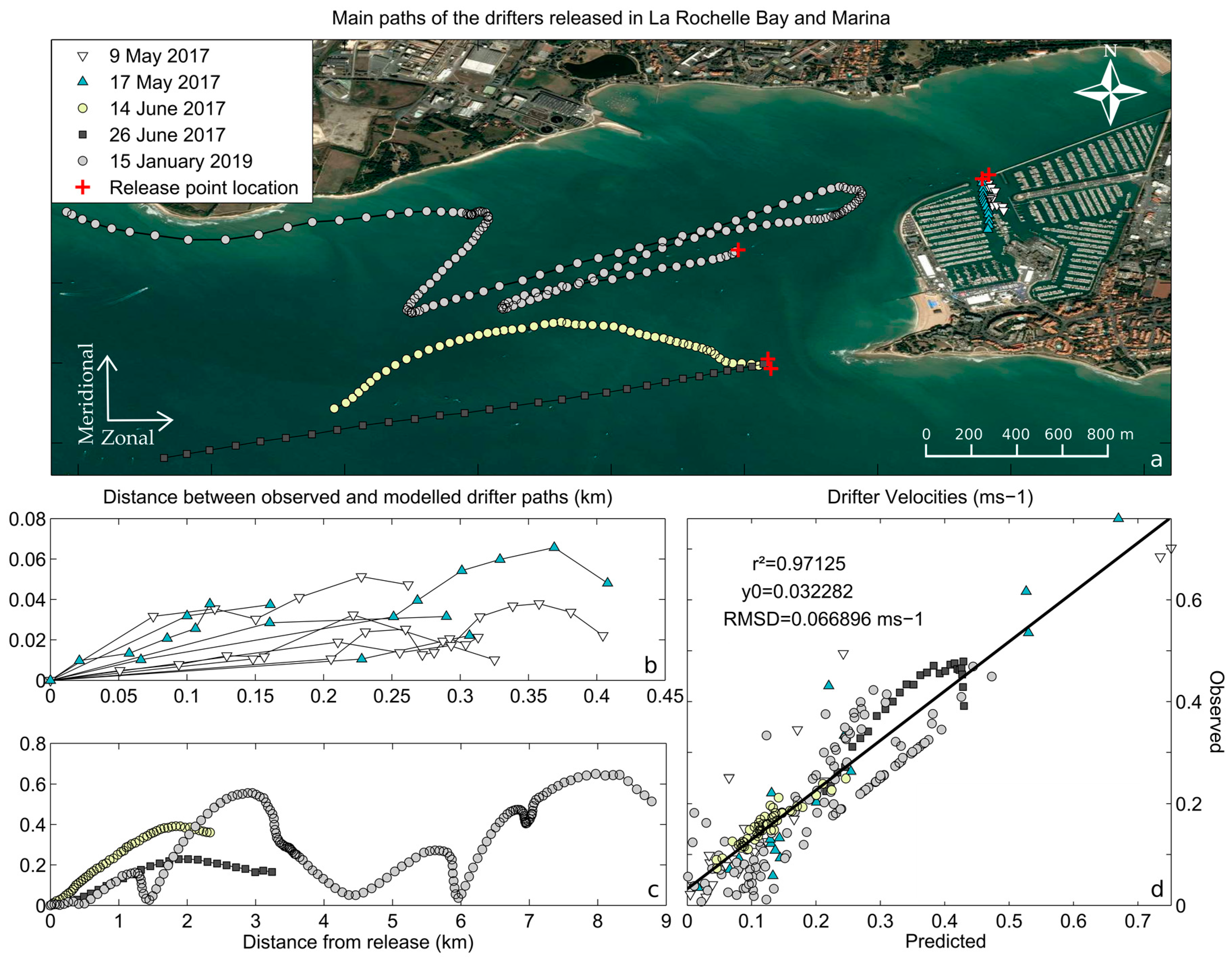
In the framework of the study, several drifting buoys were released for a wide range of temporal and spatial scales. The drifters, manufactured by Pacific Gyres (Oceanside, CA, USA), are composed of a surface float with a diameter of 0.3 m and a drogue dimension of 1.2 m length. The buoy uses Iridium to send float positions with 5-min temporal resolution. First experiments involved their deployment at the marina entrance with less than 1-h transport while the following occurred more offshore for timescales reaching more than one day. The range of hydrodynamics and atmospheric conditions tested, and the settings of the experiments were resumed in Table 2 while the mean trajectories of each drifting buoy experiment were resumed in Figure 3a. Because of maritime infrastructure and boat navigation, more release of drifting buoys was needed to track sufficient currents patterns inside the marina.
To facilitate the comparison, the real-time positions of the drifting buoys were averaged for each release while the positions of 10 simulated drifters were averaged for each corresponding release. Comparison is visible in Figure 3 and shows fair agreement between the observed and simulated circulation of the drifters. While the distance between simulated and observed drifters can reach 600 m after one day of release, the comparison indicates a good correlation in term of velocities and a 6 cms−1 Root-Mean-Squared-Discrepancy (hereafter RMSD). The meridional (V) and zonal (U) components of velocity also display a fair agreement but with less accuracy and consistency (Table 3). Globally, drifter buoy trajectories are better reproduced in the bay than in the marina, in particular during calm weather conditions where RMSD reaches 0.01 ms−1. The tide in the bay rapidly and homogeneously advected drifter buoys while complex currents and micro-scale structures at the western marina entrance caused the buoys to diverge from each other. The model is less effective at reproducing the currents at the marina entrance, but the RMSD and R2 results show a good reproducibility in particular concerning the meridional component of the velocity (Table 3). First and last deployments are characterised by stronger winds and the presence of waves in the bay. As the waves and their effects (Stokes drifts, interaction wave-currents) are not implemented in this modelling study, the quality of predictions of the model is slightly decreased (Table 3).
4. Results
4.1. Integrated Flushing Time
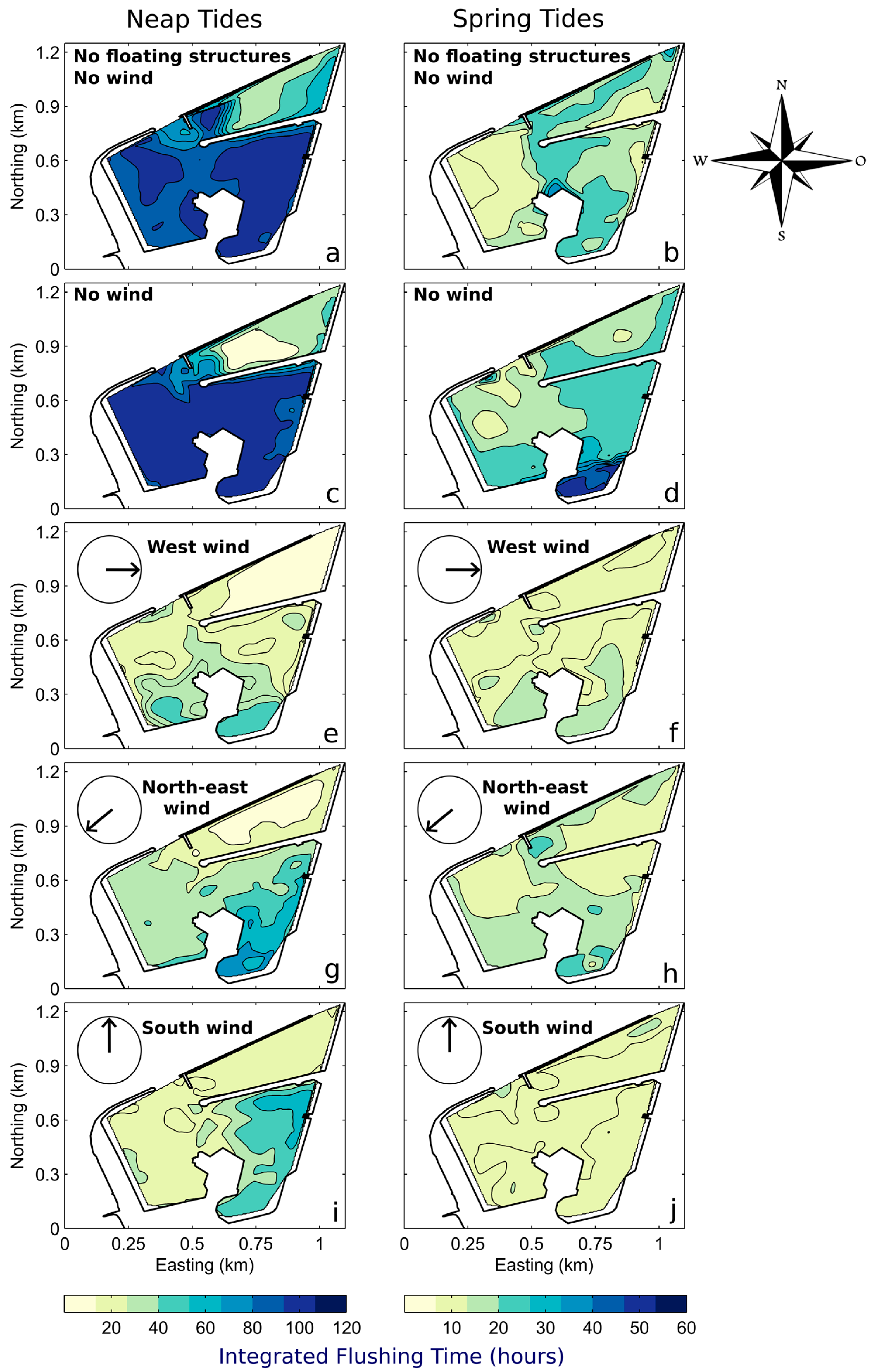
Figure 4 shows the spatial distribution of vertically-averaged Integrated Flushing Time (IFT) within La Rochelle marina for two configurations (with and without Floating Structures (FS)) associated with several combinations of wind and tide. While the first scenario considers only the tide without FS, scenarios with the wind were computed with the FS. To quantify differences between each case, we also averaged IFT (spatially and across the tidal phases) and estimated the standard deviation of its spatial variability (Spatial Standard Deviation, hereafter SSD) over the marina. We computed the standard deviation of IFT between each release (corresponding to different phases of the tide) and named it Tidal Phase Standard Deviation (hereafter TPSD).
Statistical results are visible in Table 4 while Figure 4 displays the spatial distribution of IFT. Spatially, the NE basin generally presents the lower values while the SE basin generally displays the higher values and the higher variability of IFT. IFT generally increases from the entrances to the most sheltered areas and in particular the southern part of the SE basin. The neap tide conditions exhibit 2 to 4 times larger IFT and SSD than spring tides (Figure 4, Table 4). The presence of FS increases IFT in the southern part of the SE basin during spring tides (Figure 4b–d), while it decreases IFT in the NE basin during neap tides (Figure 4a–c). While their presence slightly increases the mean IFT (23.6/22.5 h at spring tides and 89.3/88.9 h at neap tides), it considerably increases SSD during spring tides (11.1/6.2 h) and neap tides (30.2/22.7 h) (Table 4).
The wind significantly reduces IFT and SSD (on average 2 to 3 times lower) compared with situations with tide only (Figure 4c,d), in particular for the west and south directions. Although all wind cases decrease IFT in all basins relative to the tide-only case, the IFT patterns and directionality of IFT gradients vary with wind direction. For example, on neap tides the highest IFT tends to be in the southern part of the SE basin for north-east wind (Figure 4g); in the northern part of the SE basin for south wind (Figure 4i); and in the southern parts of the W and SE basins for west wind (Figure 4e). West wind is the most impacting on neap tides, and its effect increases with its magnitude. TPSD is significantly lower than SSD and is decreased by wind action and also by the presence of floating structures (Table 4). Here, we only present vertically-averaged results because the surface and bottom layers were shown to be comparable in terms of IFT (data not shown), at the scale of the marina. The relative homogeneity of the water column was found to be slightly affected by the wind.
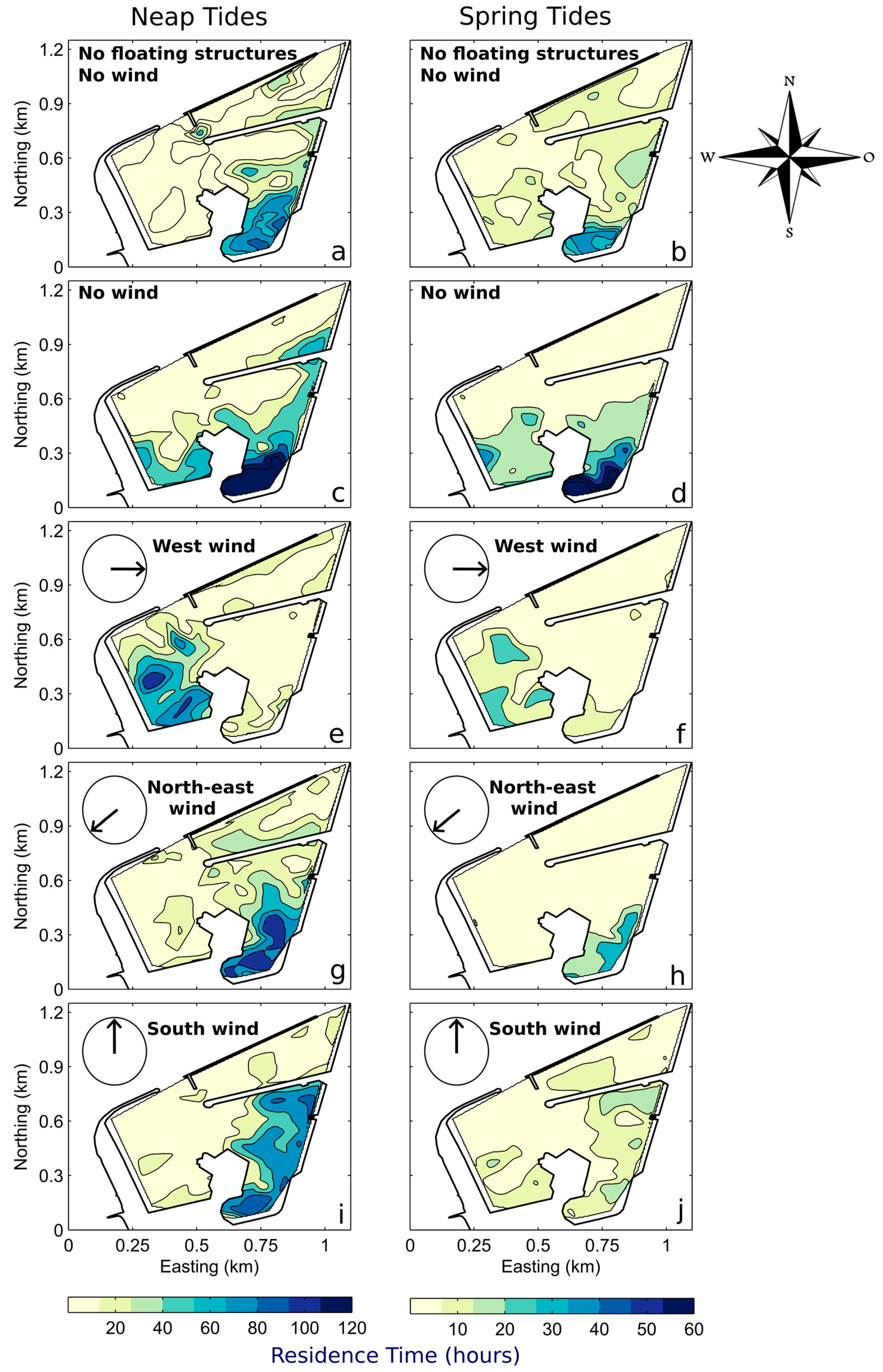
4.2. Residence Time
The vertically-averaged Residence Time (RT) of particles within La Rochelle marina is visible in Figure 5 for the same combinations of tide and wind than Figure 4. IFT and RT share many similarities, but they are quantitatively different. Mean RT is up to 3 times lower than IFT, especially for neap tides, but its spatial variability (SSD) is significantly higher.
According to Table 4, the presence of FS increases the RT (15.4/13.3 h at spring tides and 37/31.1 h at neap tides) and almost doubles SSD (20.6/12.7 h at spring tides and 42.9 h/28.3 h at neap tides). The wind has less influence on RT than on IFT and mainly reorganises RT spatially (Figure 5e–j), without substantially affecting the mean RT (Table 4). West and south winds stay the most impacting winds during neap and spring tides, respectively (Table 4). On neap tides, the lowest residence times are reached with intense 15 ms−1 west wind while on spring tides this wind configuration slightly enhances residences times compared with a 7.5 ms−1 west wind.
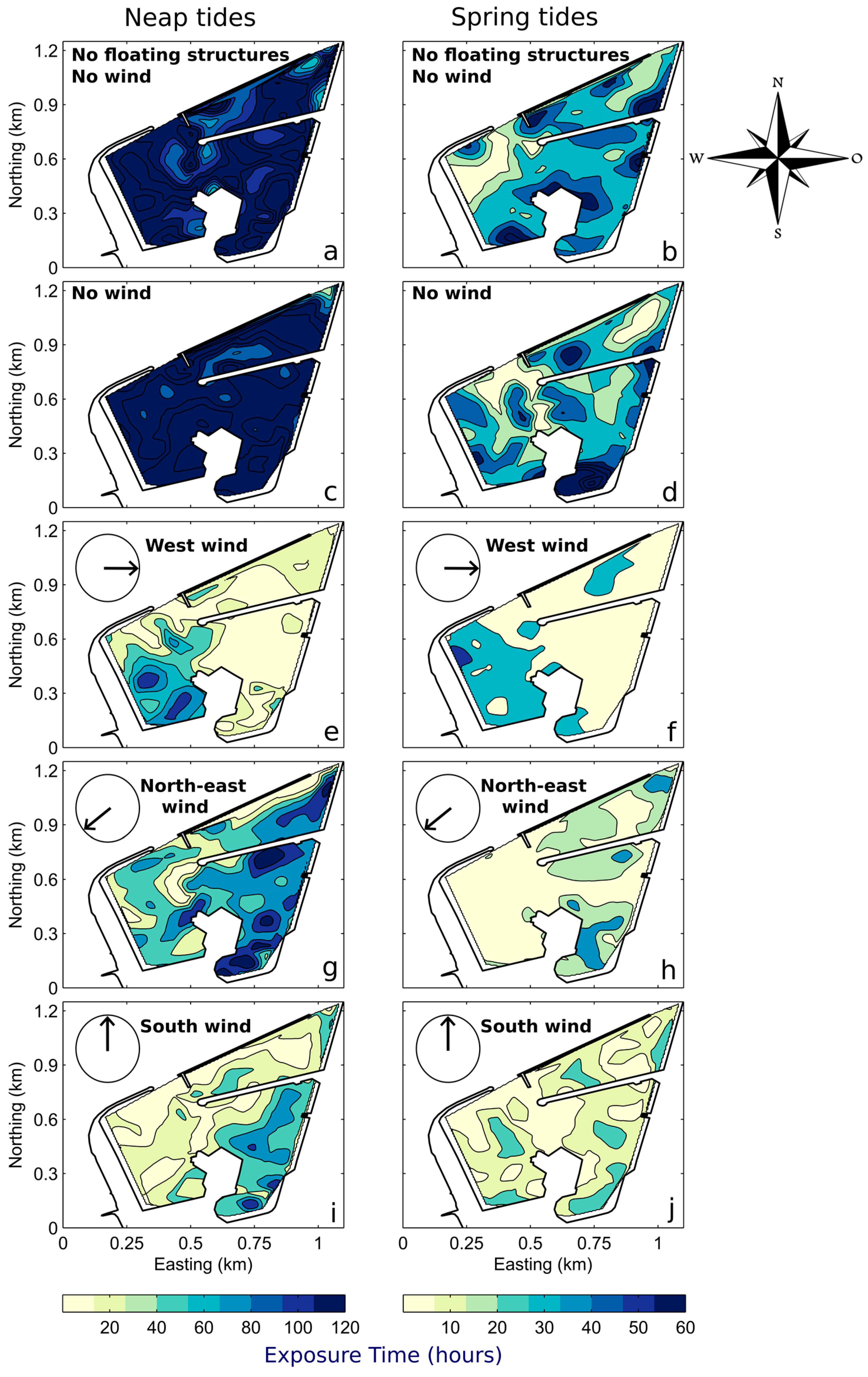
4.3. Exposure Time
The last timescale studied is ET and represents the total time that particles spend in the domain. Its computation was derived from the release of particles used to characterise RT. ET is necessarily equal to or greater than RT and is not only a function of hydrodynamic processes within the marina but also of the return-flow. Figure 6 presents the spatial distribution of the vertically-averaged exposure times computed and the statistics results related are visible in Table 4. Their behaviour share, though, some similarities with the pattern of RT and IFT but globally their magnitudes display larger values. Mean ET can significantly increase during neap tides, by doubling or almost quadrupling compared with spring tides (Table 4).
Similarly to IFT, the presence of FS does not increase significantly ET (34.8/34.5 h at spring tides and 129.3/124.1 h at neap tides). The wind has a more significant effect on exposure times than on residence times, and its impact is comparable for the behaviour of flushing times. It decreases ET by 2 to almost 5, particularly during neap tides with west winds (Table 4). Northeast winds have less influence than the other winds and mainly increase the exposure time of particles coming from both the southern part of the NE basin (on neap tides) and the entire SE basin, relative to the other wind cases. TPSD is still lower than SSD but is generally decreased by the presence of wind. During this study, we also observed that the particles returned preferentially to the marina through the western entrance (Figure 1) regardless of weather-marine conditions.
4.4. Characterisation of the Return-Flow
From the previous timescales, we assessed the importance of the return-flow in the marina through the expressions established in Section 2.3.3. The Return-flow Factor (RFF) was obtained through Equation (5) by using IFT values while the Return Coefficient (RC) was found via the Equation (7) by using RT and ET values. RFF and RC are inherently different as they were estimated, respectively, in a Eulerian and a Lagrangian way. These factors can provide relevant points of comparison that need to be analysed with caution. Results for each scenario were averaged and displayed in Table 4.
A large variety of return-flow values were found depending on the weather-marine conditions, but RFF globally displays the same behaviour than RC. The similarities mainly concern the influence of the wind and the tide. Neap tides show the higher variability of RC and RFF, with the lower and higher values respectively obtained with and without wind (Table 4). Without wind, the return-flow is always greater than 0.5, but its magnitude can drastically decrease during neap tides with the presence of wind, and particularly with the west wind (0.12 ± 0.11 and 0.19 ± 0.05 for RFF and RC, respectively). This decrease is also visible for spring tides but with less intensity (Table 4). These parameters can approach zero during intense 15 ms-1 western events. The maximum values are also obtained during neap tides without wind, with and without the presence of FS for RFF (0.73 ± 0.01) and for RC (0.75 ± 0.03), respectively. In general terms, the macro-tidal influence and the configuration of the area generate a high return-flow that is weakened under the action of the wind but not substantially affected by the presence of FS. The last result confirms the weak impact of floating structures on the circulation outside the marina.
5. Discussion
5.1. Assessment of the Main Drivers of the Water Renewal
Although the tide is a primary driver of the hydrodynamics, [19] has shown that the wind, but also infrastructures, had a substantial impact on the physical processes in the marina. The results, visible in Section 4, provide a robust view of their influence in the macro-tidal marina of La Rochelle. Here, we gather the information collected through the study of the three transport timescales to discuss the importance of the tide, the wind and the Floating Structures (FS) in the marina renewal.
5.1.1. Tidal Influence
Flushing, residence and exposure times (Figure 4, Figure 5 and Figure 6) reveal a strong spatial heterogeneity of the renewal. The NE and the SE basins generally present the lowest and largest timescale values in the marina, respectively, but the behaviour of the timescales significantly vary depending on the conditions. Close to the entrances, the water parcels are rapidly advected because of the continuous effect of the tidal currents, which decreases renewal times. On the opposite, the innermost parts of the marina are more sheltered from the flows and display the longest renewal times. This marked horizontal spatial variability has been found in estuaries and coastal embayments with macro-tidal influence [14,33,47] but also with micro-tidal influence [16,48,49].
The renewal time and its spatial variability increase as the tidal range decreases in our area: the neap tide is a very limiting factor in the renewing of waters. Indeed, tidal currents that are 3 to 4 times lower in intensity within the marina during neap tides increase the renewal time from a factor of 2–3 (for RT) to in some cases almost a factor of 4 (for IFT and ET). This result shows that the advective coastal tidal movement is a main driver of the water flow in the marina is as it was demonstrated in previous studies [40,50,51].
Other European ports investigated the behaviour of their water masses, and the results displayed a broad range of renewal timescale values. [52,53] found global flushing times of 288 and 120 h, for a Sicilian micro-tidal and an Australian macro-tidal port, respectively. In Spain, the local flushing times reached about 125 and 163 h for the meso-tidal port of Bilbao and the micro-tidal port of Barcelona, respectively [32,54]. Thus, the renewal timescales are not strictly related to the tidal regime. The shape and dimension of ports also need to be considered.
5.1.2. Wind Influence
Even if the marina is tidally dominated, the wind also has a substantial impact on the water renewal because of the presence of shallow depths. Its influence is exerted differently depending on its direction and its intensity, but the wind globally enhances the water exchange, up to a factor of almost 5 during neap tides. This significant effect on renewal timescales values has already been reported for several coastal environments [34,55,56,57,58]. The wind has a more significant influence on exposure and flushing times than on residence times, especially during neap tides (Table 4). Contrary to RT, ET and IFT take into account the return-flow into the marina. This suggests that, even if the wind has a significant influence on processes inside the marina, its impact is larger on outside processes and their interaction with processes inside the marina. It mainly pushes waters out from the marina influence and facilitates their renewal in the local environment. Among the moderate wind cases, South and west winds are the most impacting winds during spring tides and neap tides, respectively (Table 4). Water exchanges are indeed significantly enhanced by the west wind action, as reported in [19]. The effect of the south wind was less noticeable on marina flows [19], but we could explain its impact on renewal by the marina configuration. Its two main entrances (Figure 1) are almost perpendicular to the direction of propagation of southern winds which tends to evacuate water bodies more rapidly while hindering their return to the marina. The mechanisms involved during the west and south wind action are different and they are not strictly proportional to the tidal range. The funnel configuration of the bay linked to the complex architecture of the marina and the numerous tidal flats in the area could explain the non-linearity of the processes involved from neap tides to spring tides. Finally, as the variability depends mainly on the tidal forcing and the dominant wind regime, the winter which is characterised by tougher western winds, should display a faster renewal as found in [33,47,59].
The transport timescales were computed at the bottom layers, and a slight vertical variability was found in the water renewal (data not shown). With tide only, surface layers always experience the highest renewal even if the difference with bottom layers does not overpass 2 h. Even if it is less clear for north-east and south winds, west wind generally enhances the variability of the renewal between the surface and bottom layers. This result differs from the vertical heterogeneity found by some authors [32,60] that demonstrated a straight vertical variability of the renewal depending on the wind regime. In the marina, the presence of shallow depths associated with the macro-tidal forcing of the area ensure a quasi-homogeneity of the water column that is slightly affected by the action of winds.
5.1.3. Influence of Floating Structures
Floating structures (FS) have a lower influence than the wind on the total water renewal of the marina. They increase the spatial variability of the renewal by reducing the water renewal in the most sheltered parts and slightly enhancing the hydrodynamics close to the entrances [19]. With two entrances, the NE basin is particularly exposed to this enhancement. The presence of FS is also involved in the increase of the water renewal by channelling the circulation and reducing the flood-related micro-scale eddies [19]. These eddies, generated by the tide-topography interaction, develop during the flood and affect the residual circulation within the marina. Their existence can interfere with the flushing processes and subsequently generate an increase in the residence time of the particles [61]. The broad coverage of floating bodies in the marina reduces the eddy activity by decreasing velocities in the inner parts the marina and focusing it along the entrances. Although FS reduces eddies, the general decrease of currents induced is sufficient to lower the renewal of water bodies in a significant portion of the marina.
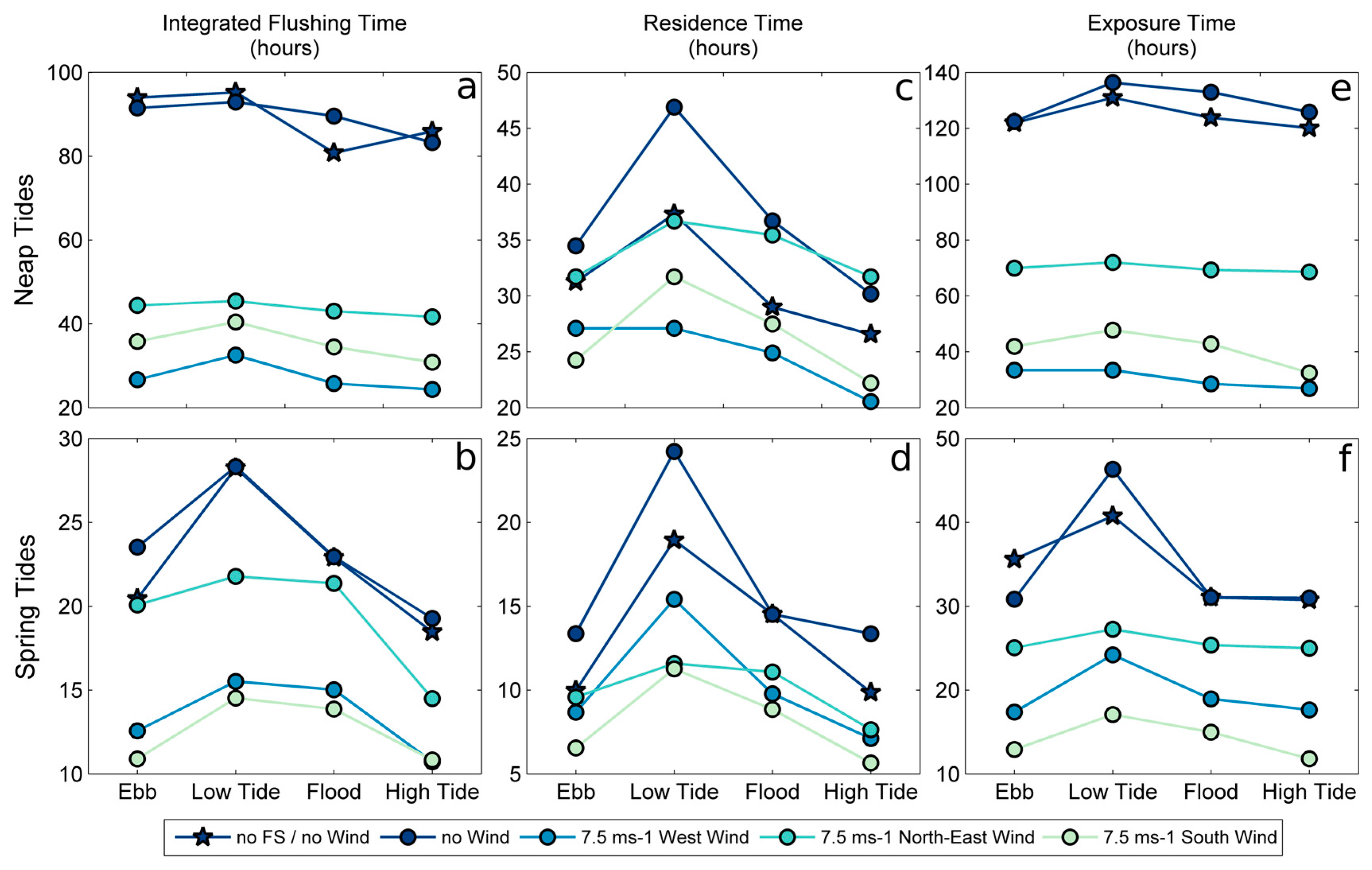
5.1.4. Influence of the Tidal Phase
Given the macro-tidal regime of the area, the tidal phase release is considered as a possible factor influencing the water transport timescales. While many studies worked with only two opposite tidal phases [44,46,57], we proposed to investigate the renewal properties of the mid-ebb, the mid-flood, the high tide and the low tide. Figure 7 enables us to investigate the influence of the tidal phase of release in the computation of the three timescale values in the marina (IFT, RT and ET).
Maximum timescale values are usually found when the release of tracer and particles occurs at low tide while the best moment to obtain lowest timescales is generally high tide (Figure 7). Generally, mid-ebb and mid-flood are quite similar in terms of renewal, even if spatial variabilities exist particularly close to the entrances. The Spatial Standard Deviation (SSD) was found to be always larger than the Tidal Phase Standard Deviation (TPSD) according to Table 4. It indicates that the variability of the renewing is more spatially than tidally dependent in the marina. Moreover, tidal phase variability of time scales generally decreased during spring tides and in the presence of wind (Table 4). This dependence on the tidal phase was already found and discussed in many studies [40,44,62].
5.2. Comparison of Water Transport Timescales
Based on the similarities shared by the several transport timescales, we highlighted general conclusions in the behaviour of the water renewal in the previous section. Here, we assess their differences to find the most relevant to describe the water transport processes occurring within the marina. The Eulerian (Integrated Flushing Time) and the Lagrangian transport timescales (Residence Time and Exposure Time) are inherently different as they follow advection-diffusion and only advection processes, respectively. The two approaches are complementary as their comparison provides exhaustive information about the motion features in the marina. As discussed in [62], their good agreement could be explained in tide-dominated environments where advection is the main driver of the circulation. Conversely, their differences in their spatial distribution characterise diffusion dominated areas. The cross-correlation of these approaches indicates that the advection mostly dominates in the marina, even if diffusion processes occur in the most sheltered parts of the marina.
The spatial distribution of Lagrangian timescales (RT and ET) displays more chaotic variability and relatively less monotonic gradients than Eulerian timescale (IFT). These chaotic patterns are the result of turbulent Lagrangian flows that generate a chaotic and non-monotonic dispersion of particles. This concept of “Lagrangian chaos”, demonstrated experimentally [63], and numerically [64], has also been experienced in [62]. It mainly contributes to greater spatial variability of Lagrangian timescales.
The Eulerian timescale IFT generally presents approximately average values between RT and ET. A sensitivity test of the « e-folding flushing time » parameter used to compute IFT (data not shown) demonstrated that the chosen percent reduction was a leading factor in the magnitude of IFT. As it was set to 63% in this study, it could help explain why IFT presents approximately average values between RT and ET. Although IFT and ET are different in terms of magnitude, they globally follow the same trend. Without wind, the transition from spring to neap tides increases IFT and ET much more than RT. It means that the combination of processes outside and inside the marina is more sensitive to the tidal range than processes occurring only in the marina. Wind influences RT less than the two other timescales. It implies that hydrodynamics within the marina are less sensitive to the wind than in the system bay-marina. RT is more vulnerable to the presence of FS than the two other timescales, which confirms that the presence of FS primarily modifies the circulation within the marina. The tidal phase release can significantly alter the time required for a water parcel to leave the marina, which noticeably affects the RT results. ET and IFT are less dependent on the tidal phase release (Table 4; compare TPSD/Mean). Considering only the tide, physical processes occurring in the marina are more sensitive to the tidal phase, while marina-bay exchanges are more tidal range dependent.
Some authors recommend to use Eulerian approaches or to take into consideration the return of particles in the system when using Lagrangian methods [40,65]. In such a macro-tidal environment, the importance of the return-flow on the water renewal requires that dynamic processes outside the area of study be considered. Taking into account the processes occurring outside the domain of study is of crucial importance to represent the water renewal of semi-enclosed tidal basins accurately. However, the computation of RT alone does not make it possible to fully characterise the behaviour of water bodies in a semi-enclosed domain with such tidal influence. In the framework of this study, the computation of IFT appears to be sufficient to represent the intra-marina exchanges as well as the exchanges between the bay and the marina. IFT and ET are also less sensitive to the initial moment of calculation, which ensures an easier solution for the calculation of currents and associated phenomena. Nevertheless, the information provided by RT was necessary to characterise the fate of waters leaving the marina via the Return Coefficient formulation. In that sense, the comparison of the three timescales allowed us to have a complete picture of the physical processes leading to the water renewal in the marina. As seen in the literature [11], the relevance of each time scale depends on the initial question and the physical, biological, and geochemical characteristics of the study area. Thus, the question of the usefulness or relevance of each timescale depends on the characteristics of the scientific study proposed.
5.3. Impact of the Return-Flow in the Water Renewal
The Return-flow Factor (RFF) and the Return Coefficient (RC) display the same behaviour while they are computed in two different ways. This consistency validates the several methods employed to characterise the water renewal in the marina. Although the three transport timescales (IFT, RT, and ET) show quantitative differences, their information allows computing the general return-flow occurring in the marina. The knowledge of the return-flow magnitude in a basin is also a straightforward way to represent the renewal by taking into account the dynamics outside the embayment. Its information and variability is a powerful indication of the water masses confinement in semi-enclosed tidal bays depending on the weather-marine conditions.
In the past, tidal prism flushing models have often set the return-flow to 0.5 or ignore it [66,67], but as suggested by [20], it should be characterised in any study. Many authors described the return-flow in different embayments throughout the world. For example, reference [68] found a maximum value of 0.15 for a micro-tidal creek in the US; reference [69] computed 0.2 to 0.9 from the entrance to the inner parts of a meso-tidal lagoon in China; reference [16] estimated a mean return-flow of 0.66 for a micro-tidal lagoon in Italy; an average return-flow of 0.32 was found by [70] in a meso-tidal Scottish Fjord; a maximum return-flow of 0.95 was reached in a meso to macro-tidal lagoon in France [33]. As experienced in La Rochelle marina and other embayments in the world, the return-flow is not correlated strictly to the tidal influence in the domain.
Here, the return flow is higher during neap tides than during spring tides in the absence of wind. The influence of the tide is particularly visible in the bay, and the back and forth movement generates significant trapping in the bay which extends to the marina. The funnel configuration of the bay and its sheltered position (Figure 1) combined with the tidal dominance of the area could explain the significant trapping of water masses, responsible for a high return-flow in the marina. This trapping is increased during neap tides when the excursions of water parcels are reduced. The study has shown that when water particles left the bay, they were rapidly ejected and their return to the system was hindered, especially in the marina. This mechanism is also described in [68], where the oscillatory flood and ebb processes caused the water masses to be trapped, particularly during neap tides. Conversely, [44] computed the larger return coefficient during spring tides, but the estuarine environment studied was much more influenced by the freshwater inputs.
The comparison of the weather-marine scenarios highlights the leading role of the wind on the reduction of the return-flow (Table 4). Neap tide conditions are particularly concerned by this decrease, which is directly correlated to lower activity of the tidal currents. The influence of the wind can overpass the tide, especially during intense 15 ms-1 west events when the return-flow can approach zero (Table 4). When water parcels leave the marina during ebb, the wind can rapidly flush them out of the bay where they are exposed to the high renewal rates of the local embayments [71].
6. Conclusions and Perspectives
The purpose of the present study was to characterise the water renewal of La Rochelle marina under a complete range of weather-marine conditions. We mainly focused on the physical mechanisms allowing to describe the renewal, but the results obtained might provide sufficient material for future studies related to the monitoring of pollutants and biological/ecological applications. Pollution is one of the major threats to water quality in coastal areas and understanding the physical behaviour of such environments is the first step toward efficient management of the problem. The results provided in this paper enable us to identify the most vulnerable zones concerning accidental pollution, but they can also be useful for undertaking protection and management policies. Results emphasise the substantial variability of the water renewal depending on the weather-marine conditions and the location in the marina.
Two different approaches helped us determining the temporal and spatial renewal of waters in the marina. The computation of three water transport timescales (IFT, RT and ET) led to the estimation of the return-flow in the marina via the RFF and RC formulations. Based on their study and comparison, the main findings concerning the water renewal in the marina are:
- The marina displays a strong horizontal variability of the renewal. The most confined waters are located in the south of the SE basin, while the NE basin is generally the most renewed.
- Both the tide and wind substantially impact the water renewal of the marina. The transition from spring to neap tides significantly decreases the water renewal while the presence of the wind enhances it, in particular for west and south directions.
- In the marina, physical processes responsible for the water renewal are generally more affected by the tidal phase than in its surrounding bay.
- The influence of the wind is less significant in the marina than in the system bay-marina.
- The water renewal is relatively homogeneous over the water column even with the effect of the wind (data not shown).
- As shown by the study of RT, the Floating Structures (FS) particularly decreased the water renewal in the most sheltered parts (SE basin), but they also generally increase it in the most exposed parts of the marina (NE basin). The study of both ET and IFT showed that they do not alter the circulation significantly outside the marina and thus, slightly affect the return-flow in the marina.
- The return-flow has been consistently represented both in a Lagrangian and Eulerian way. Its information is a relevant indication of the circulation processes occurring outside the marina. Without wind, return-flow in the marina is amplified by neap tides that generate significant trapping of the water masses at the scale of the bay. Both ET and IFT results showed that return-flow was a key parameter in the dynamics of water renewal in the marina.
- The return-flow is very sensitive to the wind action and the trapping processes happening in the bay can be drastically reduced. Wind enhances the dispersion of water masses away from the bay and thus decreases the return-flow in the marina. Powerful west winds (15 ms−1), typical of winter conditions, can generate a near-zero return-flow.
- Without wind, return-flow is amplified by neap tides that generates significant trapping.
Given the importance of the return-flow in the region of interest, we should point out that tracer mass and particles dispersion directly depend on the size of the computational domain [27,72]. We assumed the latter to be sufficiently large enough not to affect the tracer mass and the behaviour of the particles used in the definition of the water transport timescales.
The use of only one transport timescale (IFT) enabled to thoroughly describe the renewal processes occurring in the marina but also between the marina and its local environment. This parameter is less sensitive to the tidal phase release moment than RT, displays less chaotic patterns than ET and RT and offers the possibility to compute the return-flow efficiently through the tidal prism method. However, the comparison with Lagrangian timescales allowed us to detail the physical processes responsible for the renewal and to assess the consistency of the results. It underlines the need to cross-reference complementary methods and also puts forward some methods employed to address questions in a wide range of scientific domains.
Future works should characterise the influence of freshwater inflow and waves. Indeed, many authors suggested the contribution of the freshwater to the enhancement of the renewal [47,57,59,73,74]. Even if river influence is negligible in our area, intense rainy events can significantly affect the renewal times [75]. Waves that can be energetic offshore can also modify the exchange efficiency [20,76,77,78]. In the next study, the influence of dredging maintenance of the marina on the water renewal will be investigated. Indeed, the water depth was found to increase the water exchange [79], and it could be interesting to identify the optimal depth to improve the water quality of the marina.
Author Contributions
J.-R.H. and I.B. designed the study. T.C. and J.-R.H. collected and analysed the surface velocities with drifting buoys. J.-R.H. performed numerical simulations to calculate the different indicators studied. J.-R.H. analysed the results and wrote the paper. I.B. and T.C. revised the paper.
Funding
This research was funded by Région Nouvelle-Aquitaine, the direction of La Rochelle marina and the CPER (“Contrat Plan Etat Région”) DYPOMAR.
Acknowledgments
The authors wish to thank the team of La Rochelle Marina and in particular Adeline Thomassin, that provided technical support for the deployment of observing systems. The developing team of TELEMAC-MASCARET system is also acknowledged for making its code available. We also thank CNRS, Région Nouvelle-Aquitaine, and La Rochelle Université for their support and Météo France for providing us with meteorological data. The authors finally want to sincerely thank editor and reviewers chosen by Water Editorial Office, for their very constructive reviews that improved this paper greatly.
Conflicts of Interest
The authors declare no conflict of interest.
References
- Ondiviela, B.; Gómez, A.G.; Puente, A.; Juanes, J.J. A pragmatic approach to define the ecological potential of water bodies heavily modified by the presence of ports. Envion Sci. Policy 2013, 33, 320–331. [Google Scholar] [CrossRef]
- Gómez, A.G.; Ondiviela, B.; Fernández, M.; Juanes, J.J. Atlas of susceptibility to pollution in marinas. Application to the Spanish coast. Mar. Pollut. Bull. 2017, 114, 239–246. [Google Scholar] [CrossRef] [PubMed]
- Mestres, M.; Sierra, J.P.; Mösso, C.; Sánchez-Arcilla, A. Sources of contamination and modelled pollutant trajectories in a Mediterranean harbour (Tarragona, Spain). Mar. Pollut. Bull. 2010, 60, 898–907. [Google Scholar] [CrossRef] [PubMed]
- Grifoll, M.; Jordà, G.; Borja, Á.; Espino, M. A new risk assessment method for water quality degradation in harbour domains, using hydrodynamic models. Mar. Pollut. Bull. 2010, 60, 69–78. [Google Scholar] [CrossRef] [PubMed]
- Fatoki, O.S.; Mathabatha, S. An assessment of heavy metal pollution in the East London and Port Elizabeth harbours. Water SA 2001, 27, 233–240. [Google Scholar] [CrossRef]
- Bonamano, S.; Madonia, A.; Piazzolla, D.; Paladini de Mendoza, F.; Piermattei, V.; Scanu, S.; Marcelli, M. Development of a Predictive Tool to Support Environmentally Sustainable Management in Port Basins. Water 2017, 9, 898. [Google Scholar] [CrossRef]
- Mali, M.; De Serio, F.; Dell’Anna, M.M.; Mastrorilli, P.; Damiani, L.; Mossa, M. Enhancing the performance of hazard indexes in assessing hot spots of harbour areas by considering hydrodynamic processes. Ecol. Indic. 2017, 73, 38–45. [Google Scholar] [CrossRef]
- Bolin, B.; Rodhe, H. A note on the concepts of age distribution and transit time in natural reservoirs. Tellus 1973, 25, 58–62. [Google Scholar] [CrossRef]
- Takeoka, H. Fundamental concepts of exchange and transport time scales in a coastal sea. Cont. Shelf Res. 1984, 3, 311–326. [Google Scholar] [CrossRef]
- Zimmerman, J.T.F. Estuarine Residence Times. In Hydrodynamics of Estuaries, 1st ed.; Kjerfve, B., Ed.; CRC Press: Boca Raton, FL, USA, 1988; p. 171. [Google Scholar]
- Monsen, N.E.; Cloern, J.E.; Lucas, L.V.; Monismith, S.G. A comment on the use of flushing time, residence time, and age as transport time scales. Limnol. Oceanogr. 2002, 47, 1545–1553. [Google Scholar] [CrossRef] [Green Version]
- Delhez, E.J.M.; Heeming, A.W.; Deleersnijder, E. Residence time in a semi-enclosed domain from the solution of an adjoint problem. Estuar. Coast. Shelf Sci. 2004, 61, 691–702. [Google Scholar] [CrossRef]
- Deleersnijder, E.; Delhez, E. Timescale and tracer-based methods for understanding the results of complex marine models. Estuar. Coast. Shelf Sci. 2007, 74, 5–7. [Google Scholar] [CrossRef]
- Oliveira, A.; Baptista, A.M. Diagnostic modeling of residence times in estuaries. Water Resour. Res. 1997, 3, 1935–1946. [Google Scholar] [CrossRef]
- Abdelrhman, M.A. Simplified modeling of flushing and residence times in 42 embayments in New England, USA, with special attention to Greenwich Bay, Rhode Island. Estuar. Coast. Shelf Sci. 2005, 62, 339–351. [Google Scholar] [CrossRef]
- Cucco, A.; Umgiesser, G. Modeling the Venice Lagoon residence time. Ecol. Model. 2006, 193, 34–51. [Google Scholar] [CrossRef]
- Sánchez-Arcilla, A.; Espino, M.; Grifoll, M.; Mösso, C.; Sierra, J.P.; Mestres, M.; Spyroupoulu, S.; Hernáez, M.; Ojanguren, A.; Sotillo, M.G.; et al. Quay design and operational oceanography. The case of bilbao harbour. Coast. Eng. Proc. 2011, 1, 51. [Google Scholar] [CrossRef]
- Breitwieser, M.; Dubillot, E.; Barbarin, M.; Churlaud, C.; Huet, V.; Muttin, F.; Thomas, H. Assessment of the biological quality of port areas: A case study on the three harbours of La Rochelle: The marina, the fishing harbour and the seaport. PLoS ONE 2018, 13, e0198255. [Google Scholar] [CrossRef] [PubMed]
- Huguet, J.R.; Brenon, I.; Coulombier, T. Influence of floating structures on the tide and wind-driven hydrodynamics of a highly populated marina. J. Waterw. Port Coast. Ocean Eng. 2019. In press. [Google Scholar]
- Sanford, L.P.; Boicourt, W.C.; Rives, S.R. Model for Estimating Tidal Flushing of Small Embayments. J. Waterw. Port Coast. Ocean Eng. 1992, 118, 635–654. [Google Scholar] [CrossRef]
- Chaumillon, E.; Weber, N. Spatial variability of modern incised valleys on the French Atlantic coast: Comparison between the Charente (Pertuis d’Antioche) and the Lay-Sèvre (Pertuis Breton) incised valleys. In Incised Valleys in Time and Space, 1st ed.; Dalrymple, R.A., Leckie, D.A., Tillman, R.A., Eds.; SEPM Special Publications: Tarsa, OK, USA, 2006; pp. 57–85. [Google Scholar]
- Bertin, X.; Bruneau, N.; Breilh, J.F.; Fortunato, A.B.; Karpytchev, M. Importance of wave age and resonance in storm surges; the case Xynthia, Bay of Biscay. Ocean Model. 2012, 42, 16–30. [Google Scholar] [CrossRef]
- Le Cann, B. Barotropic tidal dynamics of the Bay of Biscay shelf: Observations, numerical modelling and physical interpretation. Cont. Shelf Res. 1990, 10, 723–758. [Google Scholar] [CrossRef]
- Bertin, X. Morphodynamique Séculaire, Architecture Interne et Modélisation d’un Système Baie/Embouchure tidale: Le Pertuis de Maumusson et la Baie de Marennes-Oléron. Ph.D. Thesis, La Rochelle University, La Rochelle, France, 2005. [Google Scholar]
- Dodet, G.; Bertin, X.; Tabord, R. Wave climate variability in the North-East Atlantic Ocean over the last six decades. Ocean Model. 2010, 31, 120–131. [Google Scholar] [CrossRef]
- Hervouet, J.M. Hydrodynamics of Free Surface Flows: Modelling with the Finite Element Method; John Wiley and Sons: Hobken, NJ, USA, 2007; p. 360. [Google Scholar]
- Viero, P.D.; Defina, A. Renewal time scales in tidal basins: Climbing the Tower of Babel. In Sustainable Hydraulics in the Era of Global Chang, 1st ed.; Taylor & Francis Group: London, UK, 2016; p. 216. [Google Scholar]
- Donea, J.; Giuliani, S.; Halleux, J.P. An arbitrary Lagrangian-Eulerian finite element method for transient dynamic fluid-structure interactions. Comput. Methods Appl. Mech. Eng. 1982, 33, 689–723. [Google Scholar] [CrossRef]
- SHOM. Information Géographique Maritime et Littorale de Référence. Available online: https://data.shom.fr/ (accessed on 2 July 2019).
- AVISO+ Satellite Altimetry Data. Available online: https://www.aviso.altimetry.fr/en/data/products/auxiliary-products/global-tide-fes.html (accessed on 2 July 2019).
- Choi, K.W.; Lee, J.H.W. Numerical Determination of Flushing Time for Stratified Water Bodies. J. Mar. Syst. 2004, 50, 263–281. [Google Scholar] [CrossRef]
- Grifoll, M.; Del Campo, A.; Espino, M.; Mader, J.; González, M.; Borja, Á. Water renewal and risk assessment of water pollution in semi-enclosed domains: Application to Bilbao Harbour (Bay of Biscay). J. Mar. Syst. 2013, 109–110, 241–251. [Google Scholar] [CrossRef]
- Plus, M.; Dumas, F.; Stanisière, J.Y.; Maurer, D. Hydrodynamic characterization of the Archachon Bay, using model-derived descriptors. Cont. Shelf Res. 2009, 29, 1008–1013. [Google Scholar] [CrossRef]
- Wang, C.F.; Hsu, M.H.; Kuo, A.Y. Residence time of the Danshuei River estuary, Taiwan. Estuar. Coast. Shelf Sci. 2004, 60, 381–393. [Google Scholar] [CrossRef]
- Andrejev, O.; Myrberg, K.; Lundberg, P.A. Age and renewal time of water masses in a semi-enclosed basin—application to the Gulf of Finland. Tellus A Dyn. Meteorol. Oceanogr. 2004, 56, 548–558. [Google Scholar]
- Fugate, D.C. Estimation of Residence Time in a Shallow Back Barrier Lagoon, Hog Island Bay, Virginia, USA. In Proceedings of the Ninth International Conference on Estuarine and Coastal Modelling, Charleston, SC, USA, 31 October–2 November 2005. [Google Scholar]
- Thomann, R.V.; Mueller, J.A. Principles of Surface Water Quality Modeling and Control; Harper & Row, Publishers: New York, NY, USA, 1987; p. 656. [Google Scholar]
- Zimmerman, J.T.F. Mixing and flushing of tidal embayments in the Western Dutch wadden Sea, Part I: Distribution of salinity and calculation of mixing time scales. Neth. J. Sea Res. 1976, 10, 149–191. [Google Scholar] [CrossRef]
- Dronkers, J.; Zimmerman, J.T.F. Some principles of mixing in tidal lagoons. Oceanol. Acta 1982, 4, 107–118. [Google Scholar]
- Cucco, A.; Umgiesser, G.; Ferrarin, C.; Perilli, A.; Canu, D.M.; Solidoro, C. Eulerian and lagrangian transport timescales of a tidal active coastal basin. Ecol. Model. 2009, 220, 913–922. [Google Scholar] [CrossRef]
- Spivakovskaya, D.; Heemink, A.W.; Deleersnijder, E. Lagrangian modelling of multi-dimensional advection-diffusion with space-varying diffusivities: Theory and idealized test cases. Ocean Dyn. 2007, 57, 189–203. [Google Scholar] [CrossRef]
- Delhez, E.J.M.; Brye, B.; Brauwere, A.; Deleersnijder, E. Residence time vs influence time. J. Mar. Syst. 2014, 132, 185–195. [Google Scholar] [CrossRef]
- Wolanski, E. Estuarine Ecohydrology, 1st ed.; Elsevier Science: Atlanta, GA, USA, 2007; p. 168. [Google Scholar]
- Brauwere, A.; Brye, B.; Blaise, S.; Deleersnijder, E. Residence time, exposure time and connectivity in the Scheldt Estuary. J. Mar. Syst. 2011, 84, 85–95. [Google Scholar] [CrossRef]
- Delhez, E. On the concept of exposure time. Cont. Shelf Res. 2013, 71, 27–36. [Google Scholar] [CrossRef]
- Andutta, F.P.; Helfer, F.; Miranda, L.B.; Deleersnjider, E.; Thomas, C.; Lemckert, C. An assessment of transport timescales and return coefficient in adjacent tropical estuaries. Cont. Shelf Res. 2013, 124, 49–62. [Google Scholar] [CrossRef]
- Barcena, J.F.; Garcià, A.; Gómez, A.G.; Àlvarez, C.; Juanes, J.A.; Revilla, A. Spatial and temporal flushing time approach in estuaries influenced by river and tide. An application in Suances Estuary (Northern Spain). Estuar. Coast. Shelf Sci. 2012, 112, 40–51. [Google Scholar] [CrossRef]
- Wijeratne, S.; Rydberg, L. Modelling and observations of tidal wave propagation circulation and residence times in Puttalam Lagoon, Sri Lanka. Estuar. Coast. Shelf Sci. 2007, 74, 697–708. [Google Scholar] [CrossRef]
- Ferrarin, C.; Zaggia, L.; Paschini, E.; Scirocco, T.; Lorenzetti, G.; Bajo, M.; Penna, P.; Francavilla, M.; D’Adamo, R.; Guerzoni, S. Hydrological Regime and Renewal Capacity of the Micro-tidal Lesina Lagoon, Italy. Estuar. Coasts 2013, 37, 79–93. [Google Scholar] [CrossRef]
- Yuan, D.; Lin, B.; Falconer, R.A. A modelling study of residence time in a macro-tidal estuary. Estuar. Coast. Shelf Sci. 2007, 71, 401–411. [Google Scholar] [CrossRef]
- Cavalcante, G.H.; Kjverfve, B.; Feary, D.A. Examination of residence time and its relevance to water quality whithin a coastal mega-structure: The Palm Jumeirah Lagoon. J. Hydrol. 2012, 468–469, 111–119. [Google Scholar] [CrossRef]
- Lisi, I.; Taramelli, A.; Di Risio, M.; Cappucci, S.; Gabellini, M. Flushing efficiency of Augusta Harbour (Italy). J. Coast. Res. 2009, 56, 841–845. [Google Scholar]
- Schwartz, R.A.; Imberger, J. Flushing behaviour of a coastal marina. Coast. Eng. Proc. 1988, 2626–2640. [Google Scholar] [CrossRef]
- Grifoll, M.; Espino, M.; Gonzàlez, M.; Ferrer, L.; Sánchez-Arcilla, A. Spatial residence time description for water discharges in harbours. In Proceedings of the 4th Internation Conference on Marine Waste Water Disposal and Marine Environment, Antalya, Turkey, 6–10 November 2006. [Google Scholar]
- Orfila, A.; Jordi, A.; Basterretxea, G.; Vizoso, G.; Marbà, N.; Duarte, C.M.; Werner, F.J.; Tintoré, J. Residence time and Posidonia oceanica in Cabrera Archipelago National park, Spain. Cont. Shelf Res. 2005, 25, 1339–1352. [Google Scholar] [CrossRef]
- Geyer, W.R. Influence of Wind on Dynamics and Flushing of Shallow Estuaries. Estuar. Coast. Shelf Sci. 1997, 44, 713–722. [Google Scholar] [CrossRef]
- Canu, D.M.; Solidoro, C.; Umgiesser, G.; Cucco, A.; Ferrarin, C. Assessing confinement in coastal lagoons. Mar. Pollut. Bull. 2012, 64, 2391–2398. [Google Scholar] [CrossRef]
- Du, J.; Shen, J. Water residence time in Chesapeake Bay for 1982–2012. J. Mar. Syst. 2016, 164, 101–111. [Google Scholar] [CrossRef]
- Umgiesser, G.; Zemlys, P.; Erturk, A.; Razinkova-Baziukas, A.; Mežine, J.; Ferrarin, C. Seasonal renewal time variability in the Curonian Lagoon caused by atmospheric and hydrographical forcing. Ocean Sci. 2016, 12, 391–402. [Google Scholar] [CrossRef] [Green Version]
- Warner, J.C.; Geyer, R.W.; Arango, H.G. Using a composite grid approach in a complex coastal domain to estimate estuarine residence time. Comput. Geosci. 2010, 36, 921–935. [Google Scholar] [CrossRef] [Green Version]
- Babu, M.T.; Vethamony, P.; Desa, E. Modelling tide-driven currents and residual eddies in the Gulf of Kachchh and their seasonal variability: A marine environmental planning perspective. Ecol. Model. 2005, 184, 299–312. [Google Scholar] [CrossRef]
- Ridderkinhof, H.; Zimmerman, J.T.F.; Philippart, M.E. Tidal exchange between the north sea and Dutch Wadden Sea and mixing timescales of the tidal basins. Neth. J. Sea Res. 1990, 25, 331–350. [Google Scholar] [CrossRef]
- Aref, H. Stirring by chaotic advection. J. Fluid Mech. 1984, 143, 1–21. [Google Scholar] [CrossRef]
- Arega, F.; Badr, A.W. Numerical age and residence-time mapping for a small tidal creek: Case study. J. Waterw. Port Coast. Ocean Eng. 2010, 136, 226–237. [Google Scholar] [CrossRef]
- Arega, F. Hydrodynamic modeling and characterizing of Lagrangian flows in the West Scott Creek wetlands system, South Carolina. J. Hydro Environ. Res. 2013, 7, 50–60. [Google Scholar] [CrossRef]
- Dyer, K.R. Estuaries: A Physical Introduction; John Wiley and Sons: New York, NY, USA, 1973. [Google Scholar]
- Callaway, R.J. Flushing study of South Beach Marina, Oregon. J. Waterw. Port Coast. Ocean Eng. 1981, 102, 47–58. [Google Scholar]
- Arega, F.; Armstrong, S.; Badr, A.W. Modeling of residence time in the East Scott Creek Estuary, South Carolina, USA. J. Hydro Environ. Res. 2008, 2, 99–108. [Google Scholar] [CrossRef]
- Zhang, C. Water renewal timescales in an ecological reconstructed lagoon in China. J. Hydroinform. 2013, 15, 991–1001. [Google Scholar] [Green Version]
- Gillibrand, P.A. Calculating Exchange Times in a Scottish Fjord Using a Two-dimensional, Laterally-integrated Numerical model. Estuar. Coast. Shelf Sci. 2001, 53, 437–449. [Google Scholar] [CrossRef]
- Ascione Kenov, I.; Muttin, F.; Campbell, R.; Fernandes, R.; Campuzano, F.; Machado, F.; Franz, G.; Neves, R. Water fluxes and renewal rates at Pertuis d’Antioche/Marennes-Oléron Bay, France. Estuar. Coast. Shelf Sci. 2015, 167, 32–44. [Google Scholar] [CrossRef]
- Bialik, R.J.; Karpiński, M. On the effect of the window size on the assessment of particle diffusion. J. Hydraul. Res. 2018, 56, 560–566. [Google Scholar] [CrossRef]
- Huang, W.; Spaulding, M. Modelling residence-time response to freshwater input in Apalachicola Bay, Florida, USA. Hydrol. Process. 2002, 16, 3051–3064. [Google Scholar] [CrossRef]
- Asselin, S.; Spaulding, M.L. Flushing Times for Providence River Based on Tracer Experiments. Estuaries 1993, 16, 830–839. [Google Scholar] [CrossRef]
- Malhadas, M.S.; Neves, R.J.; Leitão, P.C.; Silva, A. Influence of tide and waves on water renewal in Obidos Lagoon, Portugal. Ocean Dyn. 2010, 60, 41–55. [Google Scholar] [CrossRef]
- Azevedo, A.; Oliveira, A.; Fortunato, A.B.; Bertin, X. Application of an Eulerian-Lagrangian oil spill modeling system to the Prestige accident: Trajectory analysis. J. Coast. Res. 2009, 56, 777–781. [Google Scholar]
- Delpey, M.T.; Ardhuin, F.; Otherguy, P.; Jouon, A. Effects of waves on coastal water dispersion in a small estuarine bay. J. Geophys. Res. 2014, 119, 70–86. [Google Scholar] [CrossRef]
- Guo, W.; Wu, G.; Liang, B.; Xu, T.; Chen, X.; Yang, Z.; Xie, M.; Jiang, M. The influence of surface wave on water exchange in the Bohai Sea. Cont. Shelf Res. 2016, 118, 128–142. [Google Scholar] [CrossRef]
- Malhadas, M.S.; Silva, A.; Leitão, P.C.; Neves, R. Effect of the Bathymetric Changes on the Hydrodynamic and Residence Time in Obidos Lagoon (Portugal). J. Coast. Res. 2009, 56, 549–553. [Google Scholar]
Figure 1.
Bathymetry/topography map of the modelling domain (left) and the La Rochelle marina (right). Depths are given with respect to mean-sea-level, and the straight, bold black line indicates the shoreline in the left figure while La Pallice weather station is symbolised by a blue-bordered white star. At right, the floating docks are signified by a black line, and the maritime infrastructures are indicated by a grey line. The red-bordered white stars numbered 1, 2, and 3, represent the location of the rainwater outlet, the fairing area, and the fuel station, respectively. Western, southeastern and northeastern basins are denoted by white characters W, SE and NE, respectively.

Figure 2.
The wind regime in La Pallice station over the period 2015–2018. Winter and summer periods are also distinguished to characterise their variability in terms of direction and intensity. The legend box at right indicates the intensity of wind velocity in ms−1.
Figure 2.
The wind regime in La Pallice station over the period 2015–2018. Winter and summer periods are also distinguished to characterise their variability in terms of direction and intensity. The legend box at right indicates the intensity of wind velocity in ms−1.

Figure 3.
(a) The mean paths of drifters released in La Rochelle Bay and marina entrance; (b) and (c) The distance between observed and modelled drifter paths is displayed for every deployment; (d) Correlation of predicted-observed velocities (in ms−1).
Figure 3.
(a) The mean paths of drifters released in La Rochelle Bay and marina entrance; (b) and (c) The distance between observed and modelled drifter paths is displayed for every deployment; (d) Correlation of predicted-observed velocities (in ms−1).

Figure 4.
Spatial distribution of vertically-averaged Integrated Flushing Time (expressed in hours) within the La Rochelle marina computed for the scenario (letters) defined in Table 1. Rows characterise the wind, and FS configurations and columns correspond to the tidal regime.
Figure 4.
Spatial distribution of vertically-averaged Integrated Flushing Time (expressed in hours) within the La Rochelle marina computed for the scenario (letters) defined in Table 1. Rows characterise the wind, and FS configurations and columns correspond to the tidal regime.

Figure 5.
Spatial distribution of vertically-averaged Residence Time (expressed in hours) within the La Rochelle marina computed for each scenario (letters) defined in Table 1. Rows characterise the wind and FS configurations and columns correspond to the tidal regime.
Figure 5.
Spatial distribution of vertically-averaged Residence Time (expressed in hours) within the La Rochelle marina computed for each scenario (letters) defined in Table 1. Rows characterise the wind and FS configurations and columns correspond to the tidal regime.

Figure 6.
Spatial distribution of vertically-averaged Exposure Time (expressed in hours) within the La Rochelle marina computed for each scenario (letters) defined in Table 1. Rows characterise the wind and FS configurations and columns correspond to the tidal regime.
Figure 6.
Spatial distribution of vertically-averaged Exposure Time (expressed in hours) within the La Rochelle marina computed for each scenario (letters) defined in Table 1. Rows characterise the wind and FS configurations and columns correspond to the tidal regime.

Figure 7.
Spatially-averaged timescales values obtained for each release (at Ebb, Low Tide, Flood and High Tide) for each scenario.
Figure 7.
Spatially-averaged timescales values obtained for each release (at Ebb, Low Tide, Flood and High Tide) for each scenario.


Table 1.
Summary of the scenarios tested and analysed in the study.
| Conditions | Scenarios | ||||||||||||
|---|---|---|---|---|---|---|---|---|---|---|---|---|---|
| a | c | e | g | i | k | b | d | f | h | j | l | ||
| Tides | Neap | ● | ● | ● | ● | ● | ● | ||||||
| Spring | ● | ● | ● | ● | ● | ● | |||||||
| Wind | West 7.5 ms−1 | ● | ● | ||||||||||
| North-East 7.5 ms−1 | ● | ● | |||||||||||
| South 7.5 ms−1 | ● | ● | |||||||||||
| West 15 ms−1 | ● | ● | |||||||||||
| With floating structures (FS) | ● | ● | ● | ● | ● | ● | ● | ● | ● | ● | |||
Table 2.
The drifting buoys deployments and their corresponding settings.
| Deployment Date | Number of Drifters per Release | Number of Releases | Location | Duration | Weather-Marine Conditions |
|---|---|---|---|---|---|
| 9 May 2017 | 3 | 5 | 46°08′54.1″ N 1°10′08.0″ W | Over one flood tide | Spring tides with strong south winds |
| 17 May 2017 | 3 | 5 | 46°08′54.1″ N 1°10′08.0″ W | Over one flood tide | Neap tides with calm weather |
| 14 June 2017 | 5 | 1 | 46°08′16.2″ N 1°10′46.4″ W | One ebb tide | Neap tides with calm weather |
| 26 June 2017 | 5 | 1 | 46°08′15.8″ N 1°10′46.6″ W | One ebb tide | Spring tides with calm weather |
| 15 January 2019 | 3 | 1 | 46°08′39.2″ N 1°10′52.7″ W | 24 h | Neap tides with mixed winds |
Table 3.
Statistical analysis between the observed and predicted circulation of drifters. RMSD and linear regression analysis R2 were computed for zonal (U) and meridional (V) components of the velocity.
Table 3.
Statistical analysis between the observed and predicted circulation of drifters. RMSD and linear regression analysis R2 were computed for zonal (U) and meridional (V) components of the velocity.
| Deployment Date | RMSD (ms−1) | R2 | ||
|---|---|---|---|---|
| U | V | U | V | |
| 9 May 2017 | 0.19 | 0.15 | 0.69 | 0.75 |
| 17 May 2017 | 0.17 | 0.14 | 0.71 | 0.82 |
| 14 June 2017 | 0.01 | 0.04 | 0.91 | 0.80 |
| 26 June 2017 | 0.04 | 0.06 | 0.88 | 0.69 |
| 15 January 2019 | 0.11 | 0.17 | 0.76 | 0.72 |
Table 4.
Mean, Spatial Standard Deviation (SSD) and Tidal Phase Standard Deviation (TPSD) calculated for IFT, RT, ET, RFF and RC for the weather-marine scenarios (letters) defined in Table 1. Statistics results are in hours for IFT, RT and ET and without units for RFF and RC.
Table 4.
Mean, Spatial Standard Deviation (SSD) and Tidal Phase Standard Deviation (TPSD) calculated for IFT, RT, ET, RFF and RC for the weather-marine scenarios (letters) defined in Table 1. Statistics results are in hours for IFT, RT and ET and without units for RFF and RC.
| Parameters | Weather–Marine Scenarios | ||||||||||||
|---|---|---|---|---|---|---|---|---|---|---|---|---|---|
| Neap Tides | Spring Tides | ||||||||||||
| a | c | e | g | i | k | b | d | f | h | j | l | ||
| IFT | Mean | 88.9 | 89.3 | 27.3 | 43.6 | 35.4 | 25.6 | 22.5 | 23.6 | 13.5 | 19.4 | 12.5 | 10.1 |
| SSD | 22.7 | 30.2 | 12.1 | 19.1 | 13.5 | 13 | 6.2 | 11.1 | 3.7 | 4.9 | 3.1 | 5.6 | |
| TPSD | 6.8 | 4.3 | 3.6 | 1.6 | 3.9 | 3.3 | 4.2 | 3.7 | 2.8 | 2.6 | 2 | 2.9 | |
| RT | Mean | 31.1 | 37 | 24.9 | 33.9 | 26.4 | 23.9 | 13.3 | 15.4 | 9.3 | 10.3 | 8.1 | 9.6 |
| SSD | 28.3 | 42.9 | 26.8 | 31.2 | 26.7 | 27.9 | 12.7 | 20.6 | 7.5 | 10.6 | 5.1 | 15.4 | |
| TPSD | 4.6 | 7.1 | 3.1 | 2.5 | 4.1 | 3.8 | 4.3 | 5.3 | 3.6 | 1.6 | 2.5 | 2.8 | |
| ET | Mean | 124.1 | 129.3 | 35.5 | 69.9 | 41.3 | 27.5 | 34.5 | 34.8 | 19.3 | 19.5 | 14.2 | 11.8 |
| SSD | 24.1 | 25.7 | 27.2 | 36.2 | 27.7 | 27.6 | 17.4 | 21.2 | 14.9 | 13.1 | 9.1 | 16.7 | |
| TPSD | 5 | 6.4 | 3.4 | 1.3 | 6.4 | 6 | 6.1 | 8 | 3.9 | 0.3 | 2.3 | 5.1 | |
| RFF | Mean | 0.72 | 0.73 | 0.12 | 0.45 | 0.32 | 0.06 | 0.64 | 0.66 | 0.41 | 0.59 | 0.36 | 0.19 |
| SSD | 0.02 | 0.01 | 0.11 | 0.02 | 0.08 | 0.10 | 0.07 | 0.05 | 0.11 | 0.10 | 0.10 | 0.11 | |
| TPSD | 0.05 | 0.03 | 0.03 | 0.01 | 0.01 | 0.01 | 0.04 | 0.03 | 0.01 | 0.01 | 0.02 | 0.02 | |
| RC | Mean | 0.75 | 0.73 | 0.19 | 0.51 | 0.36 | 0.09 | 0.61 | 0.56 | 0.47 | 0.50 | 0.43 | 0.08 |
| SSD | 0.03 | 0.04 | 0.05 | 0.04 | 0.05 | 0.11 | 0.09 | 0.06 | 0.13 | 0.06 | 0.08 | 0.1 | |
| TPSD | 0.06 | 0.07 | 0.04 | 0.03 | 0.01 | 0.01 | 0.06 | 0.05 | 0.02 | 0.01 | 0.03 | 0.03 | |
© 2019 by the authors. Licensee MDPI, Basel, Switzerland. This article is an open access article distributed under the terms and conditions of the Creative Commons Attribution (CC BY) license (http://creativecommons.org/licenses/by/4.0/).
Share and Cite
MDPI and ACS Style
Huguet, J.-R.; Brenon, I.; Coulombier, T. Characterisation of the Water Renewal in a Macro-Tidal Marina Using Several Transport Timescales. Water 2019, 11, 2050. https://doi.org/10.3390/w11102050
AMA Style
Huguet J-R, Brenon I, Coulombier T. Characterisation of the Water Renewal in a Macro-Tidal Marina Using Several Transport Timescales. Water. 2019; 11(10):2050. https://doi.org/10.3390/w11102050
Chicago/Turabian StyleHuguet, Jean-Rémy, Isabelle Brenon, and Thibault Coulombier. 2019. "Characterisation of the Water Renewal in a Macro-Tidal Marina Using Several Transport Timescales" Water 11, no. 10: 2050. https://doi.org/10.3390/w11102050
Note that from the first issue of 2016, this journal uses article numbers instead of page numbers. See further details here.