On the Use of Parametric Wind Models for Wind Wave Modeling under Tropical Cyclones

Abstract

Wave and wind forces from tropical cyclones are one of the main design parameters of coastal and offshore infrastructure in tropical areas. The estimation of ocean waves parameters in the design of structures in tropical areas is difficult due to the complexity of wind fields associated with tropical cyclones. The use of numerical wave models, forced with parametric wind fields, is a common practice within the climatic characterization of extreme events. However, there is currently no consensus on the selection of parametric models for wave prediction due to the lack of a rigorous assessment of different models. In this study, six well-known parametric wind models were tested, compared, and applied in the Gulf of Mexico and the Caribbean Sea. Therefore, the evaluation and comparison of the resulting wind and wave fields are presented, showing that a particular model may best represent a specific event, but, when dealing with a large number of events, the choice of a particular parametric wind model or a combination of them does not guarantee greater accuracy.

1. Introduction

Tropical cyclones (TC) are one of the major destructive forces in nature, resulting in losses due to extreme wind speeds, precipitations, ocean waves, and storm surges. While wind and precipitation can lead to damages inland and storm surge in coastal areas, ocean waves are a relevant hazard affecting offshore areas and acting upon the storm surge as a destructive force when arriving at the coast. For example, hurricane Ivan (2004) partially destroyed seven oil and gas offshore platforms, while six drilling rigs reported major damage in the Gulf of Mexico [1], with measured waves of approximately 29 m [2]. The following year, 2005, hurricanes Rita and Katrina affected 113 oil and gas offshore platforms and seven drilling rigs, severely damaging 170 structures [3,4]. Moreover, Hurricane Katrina generated record-breaking waves with significant wave heights (Hs) of 16.76 m measured at buoy 42040 from the National Data Buoy Center (NDBC), with wave height estimations as high as 32.1 m offshore [3]. Extreme waves delivered in the 2004 and 2005 seasons led to the revision of the American Petroleum Institute (API) guidance document for hurricane conditions [5], denoting the importance of TC derived ocean waves in tropical regions and of their adequate representation.

Numerical modeling is a standard tool to derive spatial and temporal homogeneous extreme waves in tropical areas due to the scarce measured data. These models require wind fields as the primary forcing, commonly available from wind reanalysis and TC wind datasets. The main advantage of wind reanalysis is their homogeneity regarding the analysis techniques [6]. However, they are too coarse to represent extreme TC winds with high vorticity [7,8], leading to underestimation of maximum winds [9,10], and, thus, being inaccurate to derive TC generated waves [11]. Other techniques have been sought to overcome this limitation, such as wind downscaling techniques involving models capable of solving high-resolution TC wind fields (e.g., [12,13,14]). While these approaches provide accurate wind fields, their implementation is time-consuming and unfeasible for long-term analyses. Other databases, such as the Real-time Hurricane Wind Analysis System (H*Wind) [15,16], provide high-resolution measured wind fields to force wave models. However, H*Wind is only available for the North Atlantic and post-1996 hurricanes. Furthermore, the H*Wind temporal resolution between wind fields is too coarse for most long-term studies related to TC.

An alternative to accommodate historical TC in wave studies is to integrate wind parametric models to reconstruct the wind fields based on a limited set of parameters. The development of parametric wind models started with the introduction of the Rankine vortex model [17] by Depperman [18]. Later, Schloemer [19] proposed an alternative model under the concept of distributing the storm pressure in a rectangular hyperbola, from which Myers [20] derived a pressure–wind relation, and Holland [21] added a new parameter (B shape parameter) in the pressure distribution. Since then, other studies have raised modifications and adjustments to suit individual cases or locations. More recently, satellite and radar measurements motivated the revision of those models (e.g., [8,22,23]), and their parameters (e.g., the Holland-B parameter by Vickery and Wadhera [24]), while new models developed based on measurements or physical processes theory (e.g., [25,26,27,28,29,30]).

The use of parametric models is frequent due to their efficiency, simplicity, and low computational cost, hence is an excellent alternative if the driving parameters are accurately determined [31]. For instance, they are particularly useful to derive wind fields for long-term studies requiring modeling a large number of storms. Some examples of the use of parametric wind models include waves and storm surge analysis [32,33,34,35,36], wave setup estimation [37], risk modeling [38,39,40], forecasting [41,42], storm surge and waves hindcasting [43], emergency management [31], structural design [44], and analysis of trends under present climate and global warming [45,46].

Despite the widespread use of parametric models, there are only a few published studies comparing ocean waves estimated using them. Phadke et al. [31] compared three parametric wind models and evaluated TC derived waves from numerical models with buoy measurements from one TC, finding that a modified Rankine vortex provides better results for estimated wind fields but without a clear conclusion related to ocean wave fields. Jeong et al. [8] found differences of several meters of Hs between the Rankine model and a modified version. Nevertheless, based on previous studies, it is unclear which model could give better results when used for modeling TC derived waves. When dealing with few events, this is not an issue as it is possible to analyze different parametric wind models to determine which one is the most accurate (e.g., [47]). However, this is particularly problematic when dealing with a vast amount of historical or synthetic events to assess extreme wave climate conditions and wave parameters for design.

This study is presented as an extended case study of the more readily available and commonly used parametric wind models for use in wave modeling when considering a large number of events. Please note, that for a small number of events, complex models (e.g., [29,30]), may provide different conclusions than those of this study; nevertheless, their use for a large number of events is unfeasible as they require data which are not readily available for historical and synthetic events. We evaluated six parametric wind models by comparing the wind fields with ten TC events in the Gulf of Mexico (GoM) and the Caribbean Sea that reach major categories available in the H*Wind database. Subsequently, we conducted a direct comparison between numerically-obtained wave data and measurements from seven National Data Buoy Center (NBDC) buoys. We employed 13 wind field events, each one obtained with each of the six parametric models. Finally, we present a discussion about a permutation technique for each of the waves derived from the parametric models, in order to identify if a permutation method would provide better results for determining the tropical cyclones derived wave conditions.

2. Methods and Data

The main objective of this study was the assessment of different parametric wind models for use in numerical wave modeling strategy, based on two steps: (1) assessment of the accuracy of six parametric wind models to reproduce tropical cyclone wind fields; and (2) assessment of the ocean waves derived from numerical models forced by parametric wind fields. To assess the parametric model wind fields, we used H*Wind data from ten different tropical cyclones. In turn, we assessed the accuracy of the wave modeling results by using wave data from 13 events recorded by the NBDC buoys in the GoM and the Caribbean Sea.

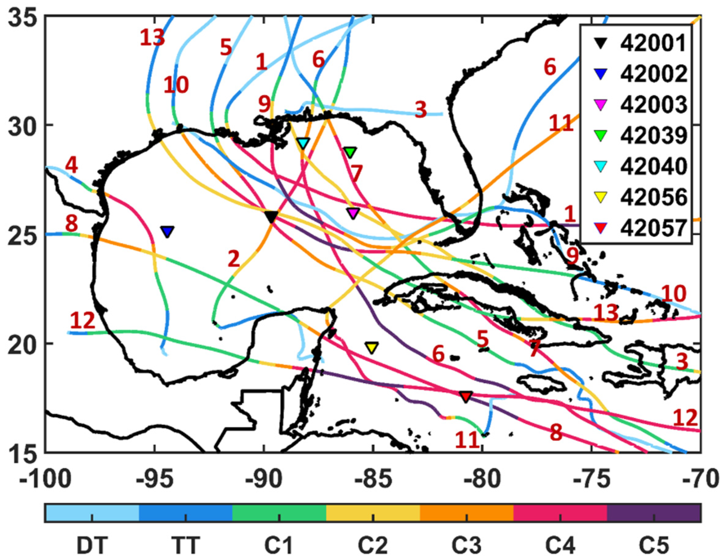
2.1. Wind and Wave Data

As input to the parametric wind models, we used the HURDAT2 data [48], which consists of 6-h temporal data for storm center location (lon-lat), maximum sustained 1-min surface wind speed (kt), central pressure (mbar), and the mean radial distance to the 34, 50 and 64 kt wind lines around the TC center. It is important to note that HURDAT2 data do not contain information about the radius of maximum wind (R_mw). While this parameter can be calculated using empirical formulas (e.g., [22,24,49,50,51]), their uncertainty is large. We then considered it more appropriate to use the R_mw available in the original HURDAT database [52]. Figure 1 shows the TC trajectories and categories for the analyzed events.

For the assessment of the parametric models derived wind fields, we used the H*Wind database (Atlantic Oceanographic and Meteorological Laboratory at the Hurricane Research Division in NOAA). This dataset ensembles multiple available surface weather observation sources (e.g., surface aviation, ships, coastal platforms, reconnaissance aircraft, anemometers, buoys, coastal stations, and satellite measurements), delivering high-resolution TC wind fields distribution in terms of u and v wind components (m/s) of the maximum sustained 1-min surface wind speeds at a 10 m reference height above mean sea level. The spatial extent of the wind fields covers an area of 8.67° × 8.68° and presents a spatial resolution of 0.0542° (~6 km). The temporal resolution between two consecutive wind fields is usually within the range of 3–7 h. Despite the uncertainty in the H*Wind product [53], it can be considered the best available TC wind field estimations (along with ocean buoys for point comparison). The H*Wind database is freely available for events earlier than 2013 at http://www.hwind.co/legacy_data/.

To assess the wind velocities and resulting wave conditions at specific locations, we used the NDBC buoy data, which include wind velocity (m/s), wind direction (°), significant wave height (m) and peak wave period (s). These data are freely available at http://www.ndbc.noaa.gov/. For buoys with anemometers at a 5 m height, the 10 m winds were calculated assuming a logarithmically varying wind profile following Mears et al. [54]. Figure 1 shows the location of the buoys, while

Table 1. Characteristics of the National Data Buoy Center buoys (NDBC) buoys used in this study at the time of analysis.

NDBC BUOYS
Buoy ID	Longitude (°)	Latitude (°)	Depth (m)	Anemometer Height (m)	Period
42001	−89.658	25.888	3246	10	1975–2017
42002	−93.666	25.79	3566.16	10	1973–2017
42003	−85.612	26.044	3282.7	5	1976–2017
42039	−86.008	28.791	307	5	1995–2017
42040	−88.205	29.205	274.3	10	1995–2017
42056	−85.059	19.874	4446	5	2005–2017
42057	−81.501	16.834	293	5	2005–2017

shows the characteristics for each buoy.

2.2. Parametric Wind Fields

Two main parameters are used in all six parametric wind models: the maximum sustained 1-min speed (V_max) in m/s and the radius of maximum wind (R_mw) in km. In addition, the Holland model [21] uses the storm central (Pc) and ambient pressure (Pn) in mbar, while the Emanuel model [27] uses an outer radius (radius to vanishing winds) (Ro) in km to limit the storm profile size. Ro is the radius at which the wind field becomes indistinguishable from the ambient flow. The computed winds fields are gradient 1-min maximum sustained speed V(r) in m/s. The following is a description of each of the parametric models assessed in this study.

1) Rankine model (RK)

Depperman [18] introduced a Rankine vortex model [17] as one of the first models describing the TC wind profile. He proposed to approximate the wind fields associated to TC by the classical Rankine vortex approximation (a center region as solid-body rotation, or constant vorticity, surrounded by circulation with zero vorticity), where the gradient speed distribution is given by Equation (1).

$$V_{\left(r\right)}=\{\begin{array}{ll}{V}_{max}\left(\frac{r}{R_{mw}}\right),& 0\le r<R_{mw}\\ V_{max}{\left(\frac{r}{R_{mw}}\right)}^X,& r>R_{mw}\end{array},$$

(1)

where r is the radial distance, and X is the scaling parameter that adjusts the velocity distribution in the radial direction [18]. The theoretical value for X is 0.5 [55,56], and typical values in the literature for X in the Atlantic and Pacific TCs are between 1/3 and 2/3 [57]. For example, Mallen et al. [58] found mean values for major TC (V_max > 50 m/s) of 0.48 and progressively smaller values for the less intense TCs. Here, we used a value of 0.5 for X.

2) Holland model (HL80)

The Holland model (1980) derives the pressure–wind profile from Myers [20] and extends the surface pressure field proposed by Schloemer [19] by introducing the B parameter to determine a modified rectangular hyperbola, as shown in Equation (2) for pressure profile and Equation (3) for wind profile.

$$P_{\left(r\right)}=P_c+\left(P_n-P_c\right){\mathrm{e}}^{{\left(-\frac{R_{mw}}{r}\right)}^B}$$

(2)

$$V_{\left(r\right)}={\left\{\left(\frac{R_{mw}}{r}\right)\left(\left(P_n-P_c\right)\frac{B{e}^{\left[-{\left(\frac{R_{mw}}{r}\right)}^B\right]}}{\rho }\right)+\frac{r^2{f}^2}{4}\right\}}^{0.5}-\frac{f r}{2}$$

(3)

where ρ is the air density, f is the Coriolis parameter (f = 2 Ω sin φ; where Ω is the rotation rate of the Earth 7.292 × 10^-5 rad/s and ρ is the latitude), e is the base of the natural logarithm and B is the shape parameter. Different models for B parameter exist in the literature (Levinson et al. [59] summarized five equations). Here we used B derived from Equation (3) at the radius of maximum gradient wind, (when r = R_mw and V = V_max):

$$B=\frac{V_{max}{}^2 \mathrm{e} \rho +f V_{max} R_{mw} \mathrm{e} \rho }{\left(P_n-P_c\right)}$$

(4)

3) Young and Sobey model (SB)

The Young and Sobey [60] wind profile model modifies the Schloemer [19] profile in the outer part of the profile where r ≥ R_mw, as given in Equation (5).

$$V_{\left(r\right)}=\{\begin{array}{ll}{V}_{max}{\left(\frac{r}{R_{mw}}\right)}^7{\mathrm{e}}^{\left(7\left(1-\frac{r}{R_{mw}}\right)\right)}& r<R_{mw}\\ V_{max} {\mathrm{e}}^{\left(0.0025 R_{mw}+0.05\right)\left(1-\frac{r}{R_{mw}}\right)}& r\ge R_{mw}\end{array}$$

(5)

4) Slosh model (SLOSH)

The storm surge model for Sea, Lake and Overland Surges from Hurricanes (SLOSH) [61] uses the parametric wind model described by Houston and Powell [62], and validated by Houston et al. [63] with H*Wind analyses. The wind profile is given by Equation (6).

$$V_{\left(r\right)}=V_{max}\frac{2 R_{mw} r}{R_{mw}{}^2+r^2}$$

(6)

5) Emanuel model (EM04)

While the previous models are partially empirical, Emanuel [27] developed a theoretical solution with a TC model based on physical environmental parameters that control the TC structure. Equation (7) describes the EM04 wind profile for r ≤ R_o.

$$V_{\left(r\right)}=V_{max}\frac{R_o-r}{R_o-R_{mw}} {\left(\frac{r}{R_{mw}}\right)}^m{\left[\frac{\left(1-b\right)\left(n+m\right)}{n+m{\left(\frac{r}{R_{mw}}\right)}^{2\left(n+m\right)}}+\frac{b\left(1-2m\right)}{1+2m{\left(\frac{r}{R_{mw}}\right)}^{2m+1}}\right]}^{\frac{1}{2}},$$

(7)

where b, n, and m are empirical parameters that control the shape of the wind profile. The model was validated against flight level observations and values of b = 0.25, n = 0.9, and m = 1.6 are commonly used (e.g., [35,64]).

The R_o parameter varies between events and during the lifetime of an event. In the Atlantic basin, R_o has a median value of approximately 400 km [65] or R_o ~ 10 R_mw for typical values of R_mw. However, Emanuel et al. [64] and Emanuel and Ravela [66] used a constant value of 1200 km, and Lin and Chavas [35] used 400 km. In this study, we used R_o = 1000 km (EM04r1000) to represent the largest TCs in the GoM and the Caribbean Sea, while we used R_o = 400 km (EM04r400) to contrast the effect of R_o over the wind profiles.

6) Emanuel and Rotunno model (EM11)

Emanuel and Rotunno [67] improved the EM04 model for the inner convective region by assuming a constant Richardson Number in the storm outflow. As the Richardson Number assumption may be violated in the outer region of the storm, the model gives an analytical gradient wind profile for V ≥ 0 (Equation (8)).

$$V_{\left(r\right)}=\frac{2 r\left(R_{mw} V_{max}+\frac{1}{2} f R_{mw}{}^2\right)}{R_{mw}{}^2+r^2}-\frac{f r}{2}$$

(8)

7) Surface Background Wind Estimation

The described parametric wind models allow determining a symmetrical wind profile for a given TC; nevertheless, TC are rarely axisymmetric, and a profile adjustment is required to create an asymmetrical wind field. To obtain the asymmetric wind field, we added the axisymmetric wind field to a uniform environmental background wind field relative to the advection of the TC. The environment background wind field is related to the storm motion [68] and is commonly related to the storm’s translation velocity (e.g., [31,41,69]). Here, we calculated the storm motion as the TC translation velocity in the free troposphere, based on the HURDAT2 data.

As the above parametric wind models generate axisymmetric wind fields corresponding to mean boundary layer or gradient winds, we needed to adjust the winds to a 10 m reference level, assess the H*Wind and buoy data, and use as forcing in the wave model. There are different techniques to compute surface winds from geostrophic winds, including atmospheric boundary layer models [70,71,72,73] and a simple wind speed reduction factor. Here, we used the parametric approach proposed by Lin and Chavas [35] where both surface wind field components are adjusted to 10 m surface level.

The method by Lin and Chavas [35] requires translating the axisymmetric component of the TC wind field and background winds to the surface 10 m reference level by considering the effect of surface friction on the storm. For the background wind field, we used a reduction factor of 0.55 over wind magnitude, and a counter-clockwise rotation angle of 22° over the direction, as described by Lin and Chavas [35]. For the axisymmetric component of the TC wind field, we employed the empirical surface wind reduction factor (SWRF) and an inflow angle following the empirical formulations by Bretschneider [74], as shown in Equation (9). Different studies show that the SWRF values vary from 0.95 to 0.65 [75], and different values are suggested in the literature. For instance, for the Holland model, Harper and Holland [76] suggested that SWRF = 0.7 and Powell [77] SWRF = 0.8, while Powell [78] suggested an SWRF between 0.75 and 0.8 and Powell and Black [79] indicated that an SWRF of 0.8 is suitable for the SLOSH wind model. Lin et al. [69] and Lin and Chavas [35] used an SWRF = 0.85 for EM11 model. For RK and SB models, we employed SWRF = 0.85 following Georgicu et al. [80] and Batts et al. [81]. The SWRF values found in the literature for each model are shown in

Table 2. Surface wind reduction factor (SWRF) employed for the wind adjustment of different parametric wind models.

MODEL	EM04	EM11	HL80	RK	SB	SLOSH
SWRF	0.8	0.85	0.775	0.85	0.85	0.8

.

$$\beta =\{\begin{array}{ll}10\left(1+\frac{r}{R_{mw}}\right),& 0\le r<R_{mw}\\ 20+25\left(\frac{r}{R_{mw}}-1\right),& R_{mw}\le r<1.2R_{mw}\\ 25,& r\ge 1.2R_{mw}\end{array}$$

(9)

Finally, the storm surface axisymmetric wind field is added to the surface background wind field. This induces an increase of TC wind speeds in the east sector of the tropical cyclone, taking as reference the direction of TC propagation, and a decrease TC wind speed in the west sector (for northern hemisphere events), therefore the resulting parametric wind field is asymmetric. In addition, it is known that the presence of two or more concentric eyewalls frequently occurs in intense symmetric TCs (e.g., [82]). Simple parametric wind models cannot reproduce TCs with a second eyewall, a secondary vortex has been included in some parametric models (e.g., [25]). However, to use those models, it is necessary to determine additional TC parameters not available in HURDAT2. Therefore, in our analysis, we only used the simple parametric wind models as described above.

2.3. Wave Model

Based on the resulting wind fields for the different selected TC, we forced the third-generation spectral wave model MIKE 21 SW [83]. A detailed description of the MIKE 21 SW model and the setup and calibration used in this work are included in Ruiz-Salcines [84] and Appendini et al. [45].

The wave model uses a directional discretization of 32 directions and a logarithmic frequency discretization with 32 frequencies with a minimum of 0.055 Hz and a factor of 1.085, using a fully spectral non-stationary time formulation. The used frequency discretization is appropriate to minimize the Garden Sprinkler effect [32,85]. For the whitecapping process characterization, we defined the dissipation coefficients Cdis and Deltadis equal to 3.5 and 0.6, respectively. The time step was automatically calculated by a multi-frequency integration step, with minimum and maximum values 0.01 s and 10,800 s. As initial condition, we defined a JONSWAP fetch growth expression with shape parameters of a = 0.07 and b = 0.09, and a peakness parameter equal to 3.3. Quadruplet-wave interactions were included for energy transfer.

The non-structured computational mesh employed covers the area of the Gulf of Mexico and the Caribbean Sea, with a varying resolution from 2 km near the NDBC buoys location to approximately 20 km in the rest of the area. The domain has close boundaries across Florida Strait (longitude 80°W) and through the islands of the Greater and the Lesser Antilles. For the water depth, we used the ETOPO 1 bathymetry [86].

3. Results and Discussion

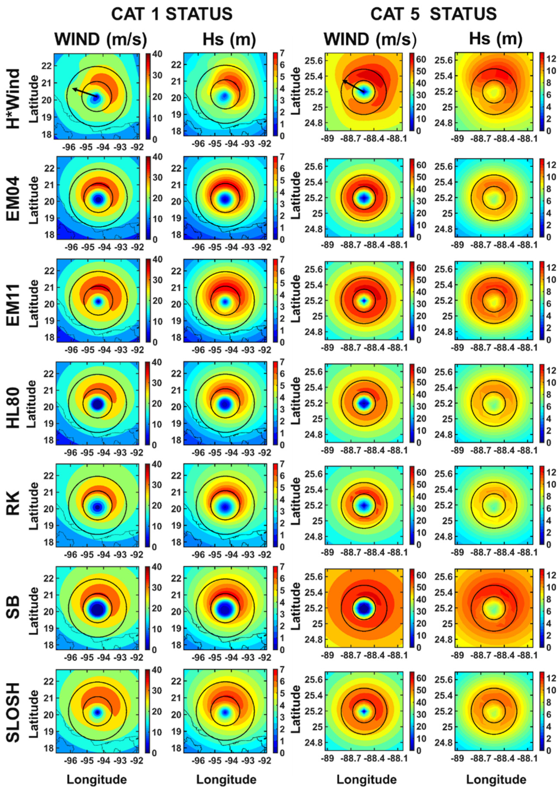
3.1. Wind Assessment

The comparison of wind profiles with wind measurements is commonly performed at geostrophic height (e.g., [30]). This implies that measured surface winds of TC (e.g., Hwind, QuickSCAT) need to be translated to geostrophic height. However, in this study, we compared the wind profiles obtained at 10 m above the surface, which is required information for wave models. At such level, the parametric wind fields become asymmetric when applying the methodology presented here. To do so, we analyzed the winds for the selected TCs (Figure 1) since wind forcing is the main parameter determining the accuracy of wave models. The TCs with Hwind available data are: Andrew 1992, Georges 1998, Lili 2002, Ivan 2004, Dennis 2005, Katrina 2005, Rita 2005, Emily 2005, Dean 2007 and Ike 2008 and only wind fields over the sea are taken account (13 wind fields for tropical storms, 40 for cat1, 37 for cat2, 45 for cat3, 56 for cat4 and 17 for cat5). Wind profiles are extracted every 22.5° (16 directions), resulting in a total of 3376 individual wind profiles for analysis. To match the time and location of the TC center, we performed a cubic spline interpolation for the HURDAT2 data before wind field calculation, to match H*Wind information. Then, we used the H*Wind location of the TC and a mesh resolution of 0.0542° to calculate the parametric wind fields. In addition, TC wind fields were rotated placing the direction of translation towards the north, to compare H*Wind and parametric wind field in each TC quadrant.3.1.1. Wind radial profile assessment.

In Figure 2, we compare the parametric normalized wind profiles for Katrina (Figure 2a) and Rita (Figure 2b) events, during category 1 (cat1) and 5 (cat5) status, respectively.

Table 3. Relative wind speed (V/V_max) percent decay at different relative radius (r/R_mw).

r/Rmw	EM04r1000		EM04r400		EM11		HL80		RK		SB		SLOSH
	C1	C5	C1	C5	C1	C5	C1	C5	C1	C5	C1	C5	C1	C5
1.5	16.0	15.2	18.8	16.5	9.4	8.1	9.3	10.3	21.6	21.6	6.9	4.7	7.7	7.7
2	32.6	31.2	37.0	33.3	23.6	20.9	21.9	24.0	34.0	34.0	13.3	9.2	20.0	20.0
2.5	43.9	42.2	49.6	44.8	36.4	32.3	32.9	35.2	42.3	42.3	19.3	13.5	31.0	31.0
3	52.0	49.9	58.6	53.0	47.1	41.7	41.9	44.0	48.3	48.3	24.8	17.5	40.0	40.0
3.5	58.0	55.7	65.4	59.1	56.0	49.3	49.4	50.9	52.8	52.8	30.0	21.4	47.2	47.2
4	62.6	60.1	70.7	63.9	63.4	55.4	55.6	56.5	56.5	56.5	34.8	25.1	52.9	52.9
5	69.5	66.6	78.6	70.9	75.2	64.8	65.5	65.0	61.9	61.9	43.5	32.0	61.5	61.5
6	74.3	71.2	84.4	75.9	84.4	71.6	72.8	71.1	65.9	65.9	51.0	38.2	67.6	67.6

summarizes the normalized wind speed (V/V_max) percent decay at different normalized distances from the TC eye (r/R_mw). The results show that EM11 and SLOSH present the highest normalized wind speed increase with normalized distance in the inner region (from TC center to R_mw), followed by EM04. RK show the lowest increases of normalized wind speed with normalized distance and with a linear trend. HL80 and SB show the largest TC eye size (location of calm winds, V/V_max ~ 0) reaching extensions of 25% R_mw for cat5 and 22% and 30% R_mw for cat1, approximately. From there, HL80 shows a steep increase in normalized wind speed with normalized distance, surpassing RK and EM04 at 50–60% V_max, approximately. SB shows a lower increase than HL80. In the areas of strong inner winds in the eyewall (the inner region near R_mw), the EM11 and SLOSH present higher normalized wind speed, being HL80 similar to EM04 in cat5 and higher than EM04 in cat1. The RK and SB models show the lowest normalized wind speed in this area.

Beyond the eyewall, SB shows higher normalized wind speeds and more extended wind decay when compared to the other models (minor than 51% of V_max at 6 × R_mw). For wave modeling purposes, SB will then have a wider area of high wind speeds generating ocean waves, which most likely result in an overestimation of wave heights. Taking into account the rate of normalize wind speed decay with the distance from the TC center, RK and EM04 are the models that present the highest rate of normalized wind speed decay in the central region (from R_mw to 2 × R_mw), with a 21.6% decay of V_max at a distance of 1.5 × R_mw for RK and 15.2% for EM04. The SLOSH, HL80, and EM11 models show quite similar profiles in the central region, although wind speed profile associated with HL80 model decays with a higher rate under weaker categories and SLOSH model decays with a lower rate during cat5. In the outer region (with distances from TC center > 2 × R_mw), RK shows the lowest decay rate follow by SLOSH under cat1 conditions and SLOSH and EM04 with larger Ro for cat5, while EM11 is the fastest decaying model for cat1 and HL80 for cat5. In the case of the EM04 models, employing lower Ro values implies a greater decay of the wind speed with increasing normalized distance. These differences demonstrate the importance of considering the evolution of Ro with time, particularly under weak category conditions. Nevertheless, the HURDAT2 data do not provide the temporal evolution of Ro, hindering the use of EM04 model.

To assess the accuracy of the surface winds given by parametric wind models, we compared radial wind speed profiles of H*Wind, and parametric wind fields, from tropical storm category to cat5 and at each 22.5° (16 directions), considering the track direction as the reference. Figure 3 shows a subset of radial profiles comparison between parametric and H*Wind radial speed profiles per category. In general terms, parametric models do not include the effect of the environmental wind shear, environmental conditions (e.g., [87,88,89,90]), non-uniform surfaces (e.g., [91]) and land–sea friction contrast (e.g., [92]). Therefore, the large asymmetries shown by H*Wind wind speed profiles cannot be represented in many cases, resulting in significant biases in the wind speed intensity and V_max location. The following patterns emerge from the results:

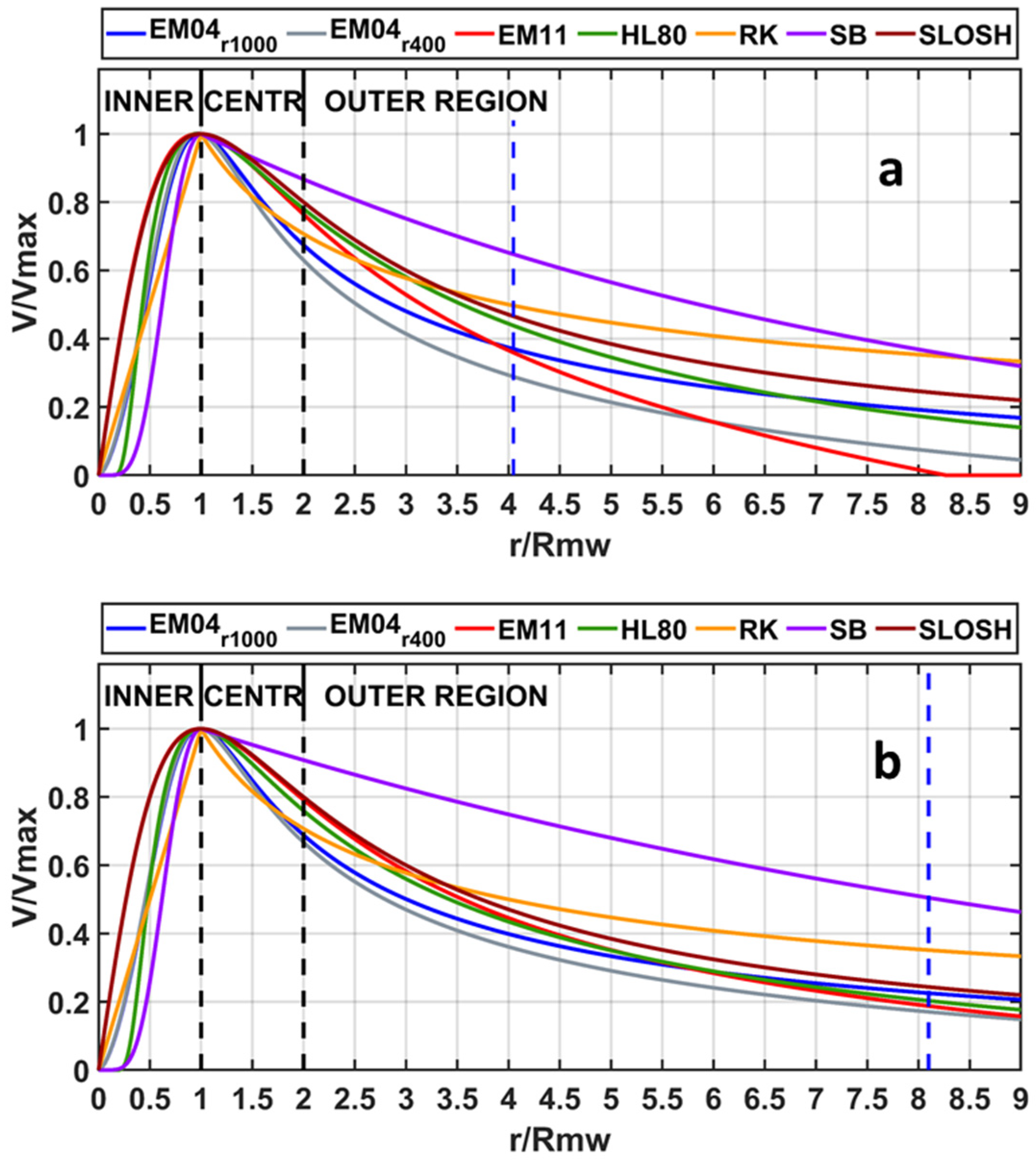
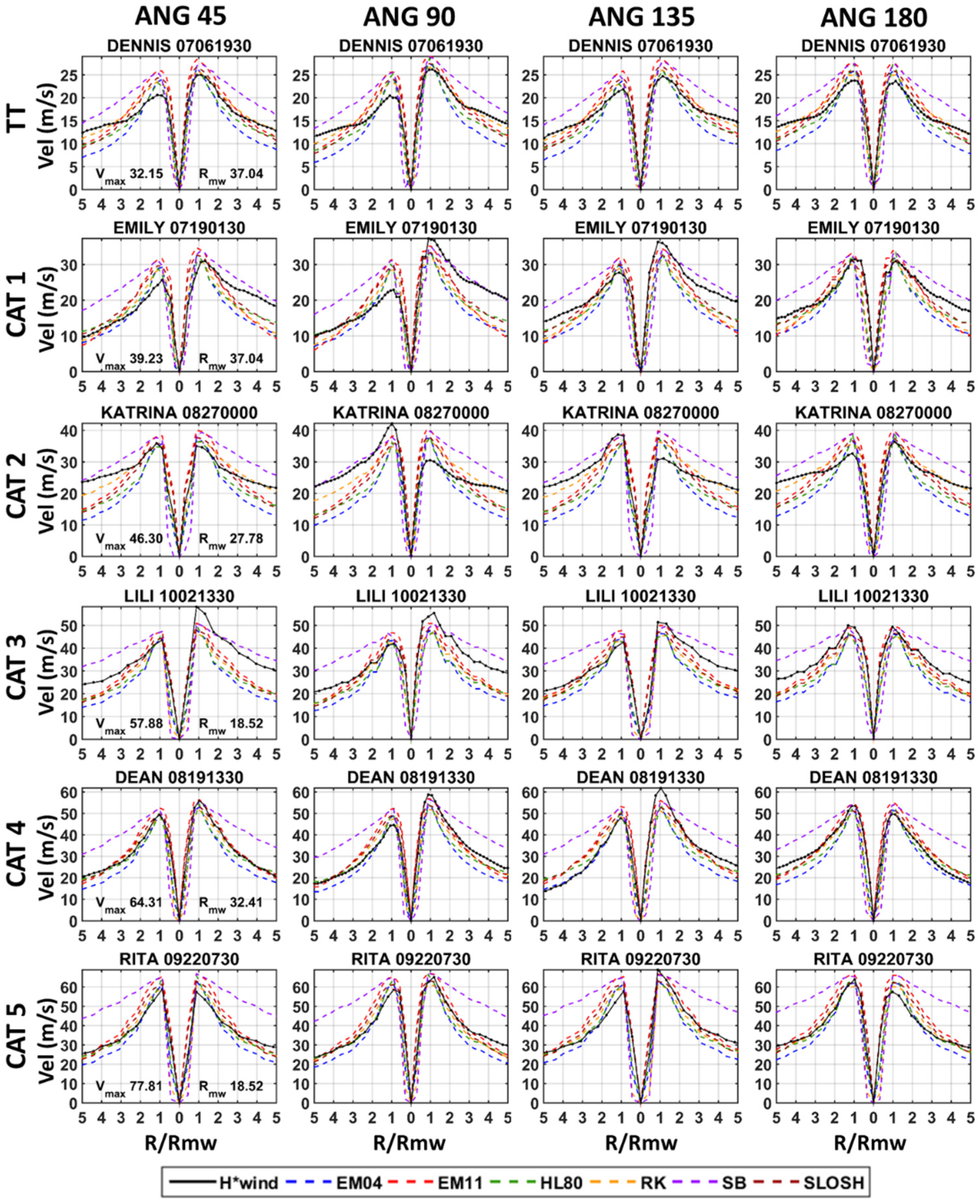
• Generally, the HL80 and SB models overestimate the size of TC eye.
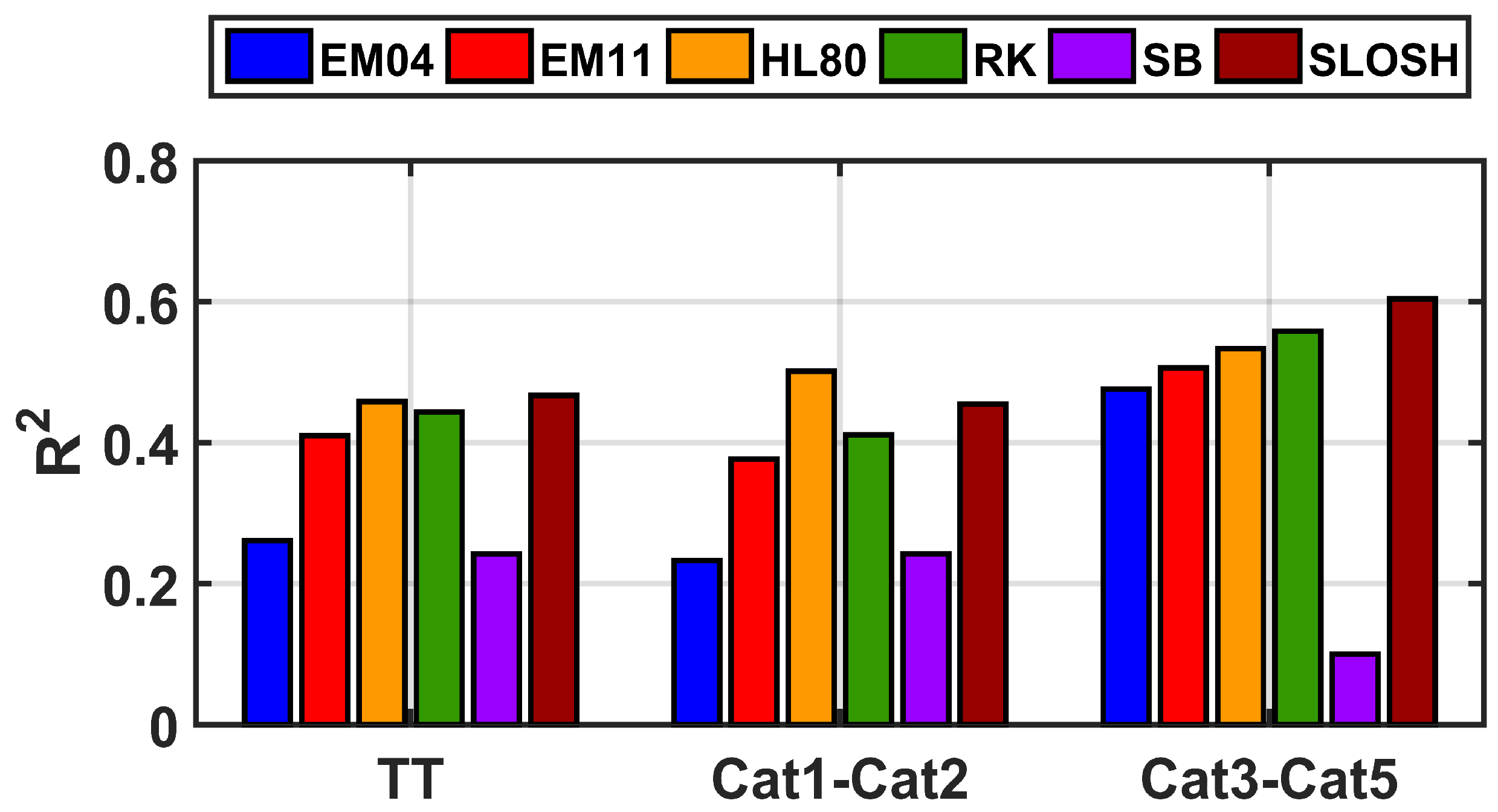
• The EM11 and SLOSH models show the most accurate fit for the inner area of the wind speed profile during major category events.
• The SB model overestimates the winds in central and outer regions of the profile for high categories, showing good agreement only for some periods during cat3 or minor categories when the wind profile decays slowly with radius in outer areas.
• For less intense events (cat1 and cat2), the EM04, HL80, and RK models show the best fit with H*Wind radial profiles, with a better representation of the central region in comparison to the outer region.
• In general, no model accurately represents the outer region (beyond 2–3 R_mw), where generally the wind profiles decay too fast.

Figure 4 shows the mean coefficient of determination (r²) associated with all wind profiles grouped in tropical storms, minor categories (cat1 and cat2) and major categories (cat3–cat5), comparing the model results with H*Wind. In general, all models except SB improve their r² with the increase of the TC category. SLOSH, HL80, RK, and EM11 shows similar r² for TT (0.41–0.47) while HL80 shows the highest r² in minor categories (0.50) followed by SLOSH and RK (0.45 and 0.41, respectively). For major categories, SLOSH is most accurate (0.60) followed by RK, HL80, EM11 and EM04 (0.56, 0.53, 0.50 and 0.48, respectively). EM11 and RK show similar results for all categories and EM04 only show good results for major categories. SB shows a very low r² in all cases. As a general conclusion, the SLOSH model is the most accurate model for these cases.

Temporal and Spatial Distribution Assessment

To analyze the spatiotemporal accuracy of the wind fields, we performed statistical analysis based on the root-mean-square error (RMS) and correlation coefficient (CC) of wind speed time series extracted from the wind fields. We extracted the time series at 22.5° intervals and over eight points located at different distances from the TC center. Figure 5 shows the boxplot representation of the time series of RMS (right panels) and CC (left panels), grouped by time series located on the right (from 0° to 180°), left and all quadrants (ALL) at different distances from TC center. The top panels are the results for all the time series.

The EM11 and SLOSH models perform better in the inner region (between 0.3 and 1 R_mw) and for the east side quadrants in the first half of the central area (up to 1.5 R_mw). Between 1.5 R_mw and 3 R_mw, HL80 model shows the lowest RMS, while RK does it for the more remote areas (above 4 R_mw). In turn, although the SB model can represent the wind fields in some cases, it provides the least accurate results in all quadrants. When considering the median of the RMS and CC of the total results (Figure 5, top panels), the boxplots show that the SLOSH model presents the lowest median of RMS and CC (7.1 m/s and 0.82), followed by HL80 and EM11 (7.3 m/s and 7.6 m/s and the CC). Finally, RK and EM04 have a median of RMS of 7.9 and 8.6 m/s, respectively, while SB has 11.6 m/s, where those three models have a similar median of CC (between 0.79 and 0.8). Nevertheless, EM11 and SLOSH present the lowest variability (the difference between percentiles 75% and 25%) in RMS (2.4 and 2.3 m/s, respectively) and CC (0.15 and 0.16) followed by EM04 (4.9 m/s and 0.23), RK 5.4 m/s and 0.23), HL80 (6.1m/s and 0.3) and SB (10.8 m/s and 0.53). Thus, EM11 and SLOSH models are more likely to better represent the TC wind fields, mainly in areas close to the V_max, when a large number of TCs are under assessment.

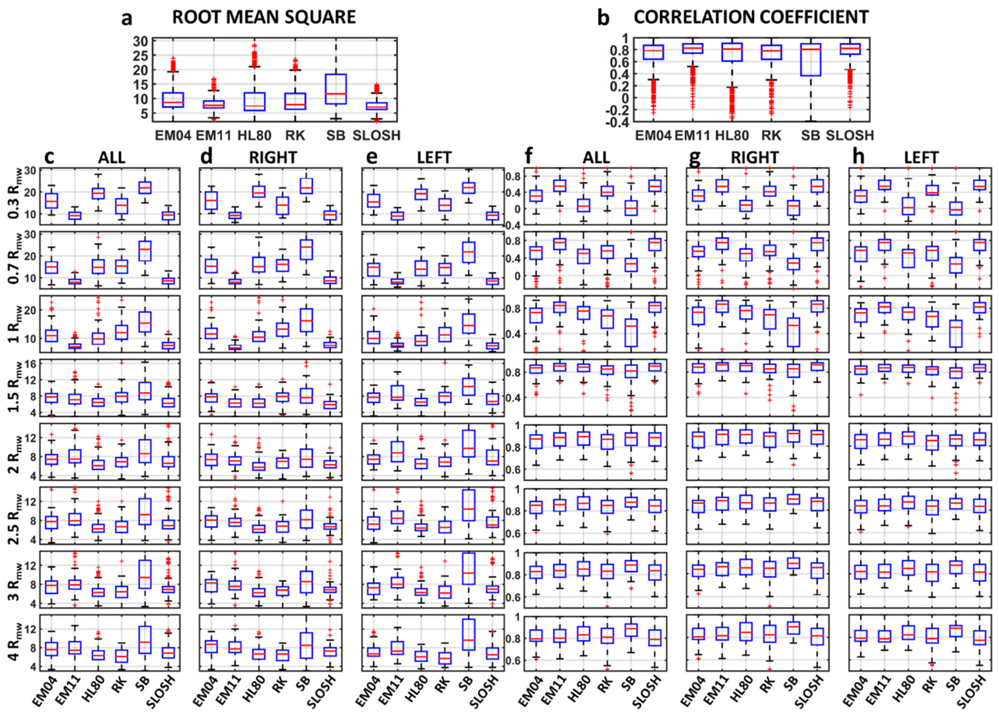
3.2. Wave Assessment

Here, we present the evaluation of the different parametric wind models based on their use for wave modeling, by comparing the spatial distribution of the generated waves and the time series with the specific buoy measurements.

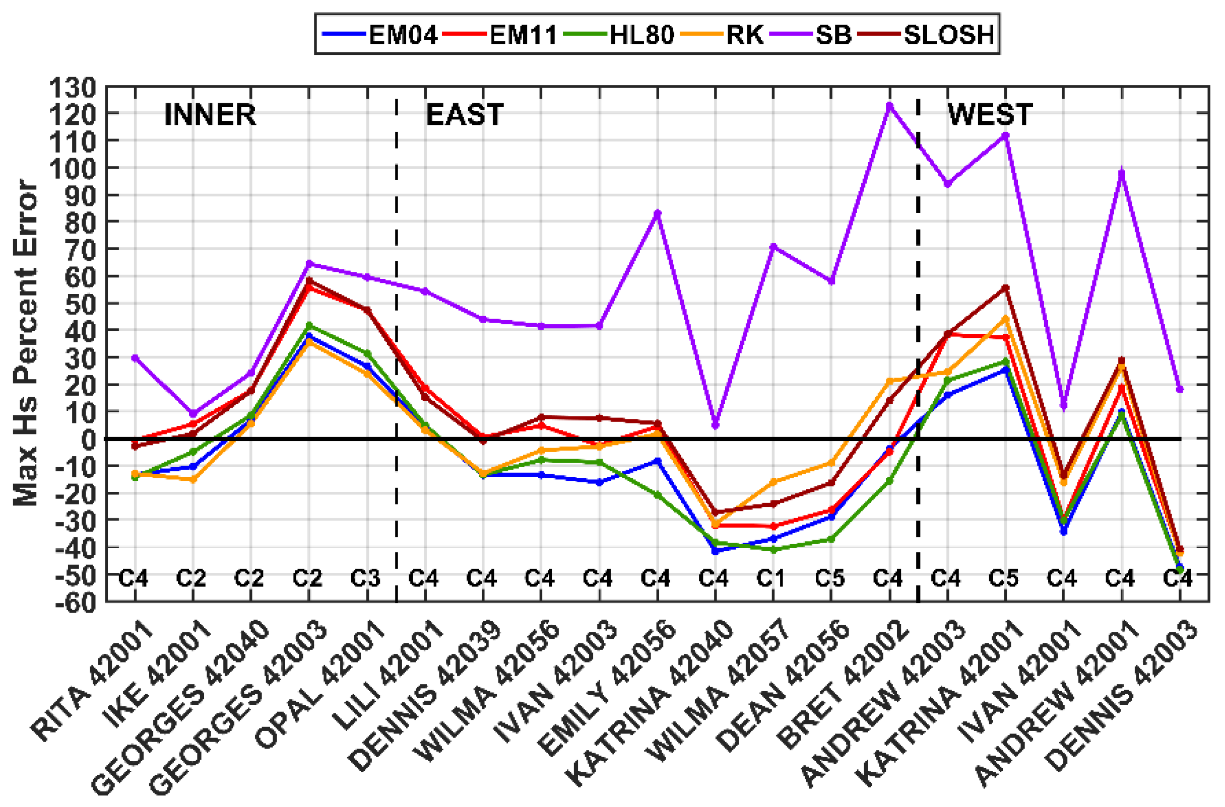
3.2.1. Spatial Distribution Assessment

We used steady-state simulations for two events, Dean (2007) during category 1 and Rita (2005) during category 5, to analyze the wave field generation from different parametric wind models. The spatial distribution of the wave field for steady-state TCs are expected to resemble the wind field pattern, so the spatial distribution of Hs error is directly related to the capacity of the wind model to represent the TC winds. Figure 6 shows both the H*Wind and parametric wind fields (first and third columns), and the wave fields generated from H*Wind and parametric models (second and fourth columns), during hurricanes Dean (cat1) and Rita (cat5). In addition, as a reference, we include the H*Wind wind and Hs fields used for biases estimation in the first panels row. The overestimation of the Hs generated from parametric wind fields reaches maximum values of 1.8 m, associated with SB model during cat5 conditions, and 1.7 m associated with the EM11 model during cat1 conditions. These overestimated values correspond to 14.4% and 26.7% higher than the Hs generated from H*Wind wind fields, respectively. Similarly, the highest Hs underestimations are 3.3 m (51.1%) using the SB during cat1 conditions and RK with 3.1 m (25%) during cat5 conditions. In general, differences in the modeled wind fields are related to differences between the wind fields of H*Wind and the parametric models, showing that the parametric wind models cannot represent TC wind fields when the driving parameters are inaccurate, as shown by Phadke et al. [31]. From the results, we found that the relationship between wind and maximum Hs errors is larger in weak categories, suggesting that a correct definition of the V_max parameter may be more relevant during weaker categories.

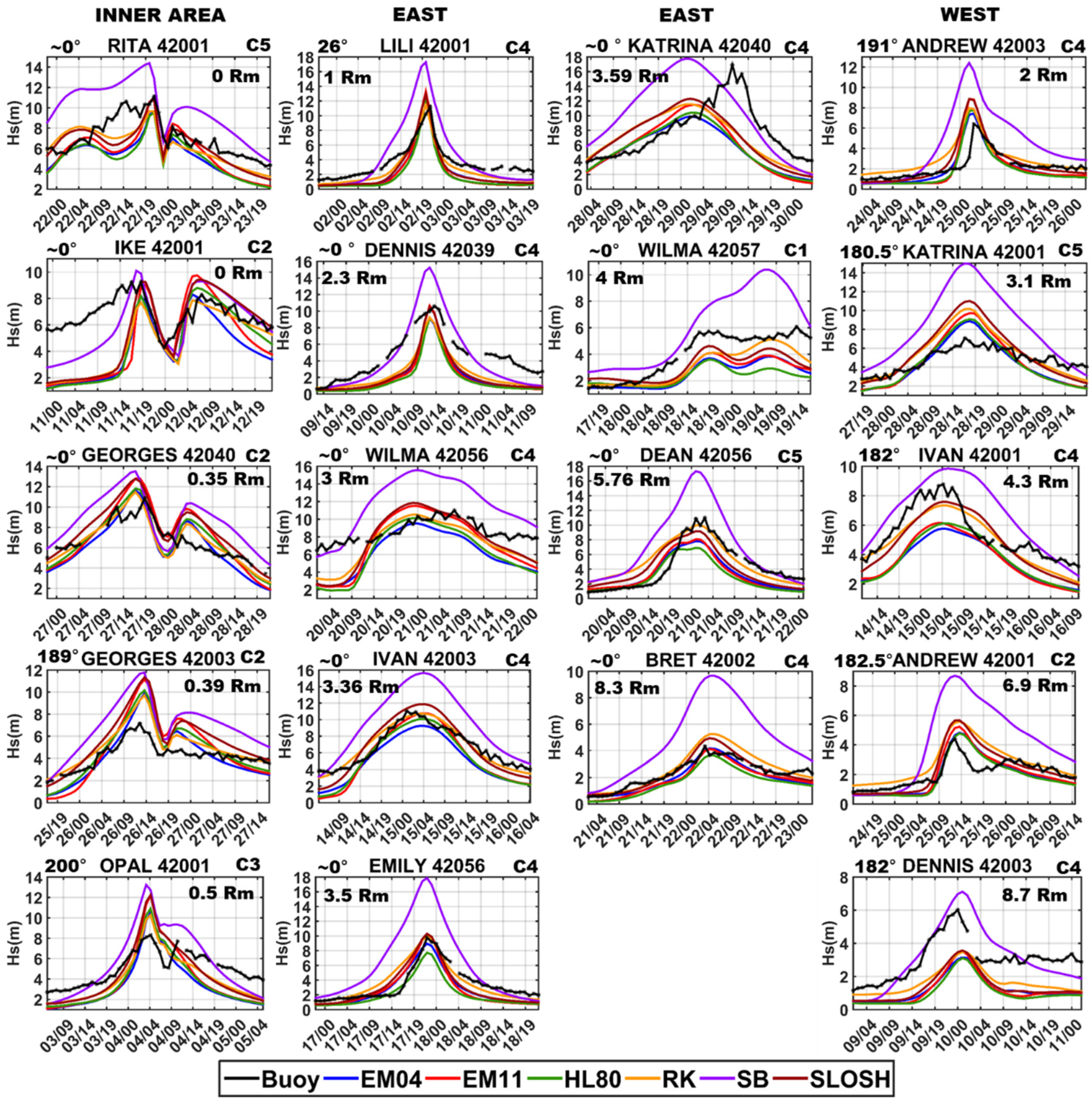
3.2.2. Wave Time-Series Assessment

We selected 13 TC and considered seven NDBC buoy locations in deep water to verify the accuracy of the wave modeling within the GoM. To avoid errors in the predicted wind fields due to land-induced asymmetries, we selected only offshore buoy data. We also considered an intersection buffer of 200 km from each buoy with the TC trajectory, so that the resulting number of cases analyzed is 19.

Figure 7 shows the resulting Hs time series for each TC using the different parametric wind fields. During TC Katrina, the Hs time series waves do not reproduce the NDBC measurements accurately, mainly due to the highly asymmetrical wind fields near the buoy. We observed the same effect for Ike after passing over buoy 42001. Another factor reducing the accuracy of the results is the formation of a second eyewall, observed during TC Katrina and Rita, which the parametric models are unable to reproduce. In particular, Katrina shows a second eye formation 60 km from the TC center that shows higher winds than in the inner eyewall [16]. Rita presents a second eye formation after crossing buoy 42001 (e.g., [93]). Furthermore, the uncertainty of the eye location also reduces the accuracy of the results [48]. Such uncertainty has an impact on the position of the wind field and, therefore, on the associated swell. For example, for Georges and Opal (at buoys 42003 and 42001, respectively), the modeled Hs has two peaks that are not seen in buoy measurements, implying that the parametric wind field has the eye moving above the buoy.

Figure 8 shows the corresponding root mean square error (RMS) and correlation coefficient (CC) when comparing model results to buoy data. The results show that SB has a poor performance, showing an overall overestimation of Hs (Figure 7) and, with few exceptions, the largest RMS (Figure 8). Excluding SB, we found a maximum difference between RMS of 1.1 m and a mean difference of 0.63 m, while a maximum difference between CC equal to 0.1. The model with the lowest RMS is RK, performing better in 47% of the cases and when the buoy is located in the inner (60%) and east zones (55.5%). When the buoy is located in the west area, EM04 performs better in three of the five cases. Nevertheless, RK has the slowest decaying wind speed rate, so that the winds remain higher far from the eye when compared to other models. As a result, RK generally performs better than the other models when simulating waves when the TC is far from the buoy, resulting in a low RMS (Figure 8), but does not necessarily provide an accurate representation of the TC highest waves (Figure 9). This is observed in the results when the TC approaches or moves away from the buoy (e.g., Rita on the buoy 42001 in Figure 7) and when the buoy is far of the TC eye, mainly when the buoy is at the east of the TC (e.g., Dean and Bret on the buoys 42056 and 42002 on Figure 7).

The relative position between the buoy and the TC track influences the accuracy found between wave model results and measurements. As such, this relative location will also affect the accuracy of the wave results. Nevertheless, there is no clear relation between the accuracy of the wave model results and the parametric wind fields used depending on the location of the buoy and the wind intensity.

Considering that the maximum Hs (Hs_max) attained at a particular event is the main parameter used for extreme value analysis to determine design parameters, we proceed to assess such parameter for each event. Figure 9 shows the Hs_max error percentage between model results and measurements. The results show that the SB parametric winds generate the highest Hs_max error, with large overestimations. When the buoy is located in the inner region and the east zone at less than three times R_mw, all models have similar behavior. EM11 and SLOSH models show lower Hs_max percent error for Rita and Ike, but higher errors than using EM04, HL80 and RK for Georges and Opal. For the east and west zones, the accuracy of the models also varies for each case and intensity. Some models improve the results depending on the distance to the buoy and the intensity of the event, although without a clear trend. Therefore, it is not possible to determine the most accurate model for all cases when considering Hs_max.

Figure 10 summarizes the accuracy of the wave modeling results based on the Hs_max, RMS, and CC boxplot of the time series. For Hs_max percent error, RK shows the best fit for all areas (Figure 10a) followed by EM11 and SLOSH. SB shows large overestimations and HL80, and EM04 underestimate the median despite showing relatively good results. In the inner region (Figure 10b), RK also shows the better fit, although EM04 has a very similar distribution, and it is followed by HL80. For the east area (Figure 10c), RK also provides the best fit, followed by SLOSH and EM11. The largest overestimations of Hs_max was by SB, including all cases and all areas. The lowest RMS error (Figure 10e–h) is obtained by the RK model, followed by SLOSH, EM04, EM11, and HL80, which have similar distributions, while SB has a larger RMS than all other models. For the CC (Figure 10i–l), the values are very similar, although they are higher for EM04, which shows a distribution with low dispersion around 0.85. Similar to the analysis for Hs, we analyzed time series of mean and peak wave period as part of our study, obtaining similar results (not shown).

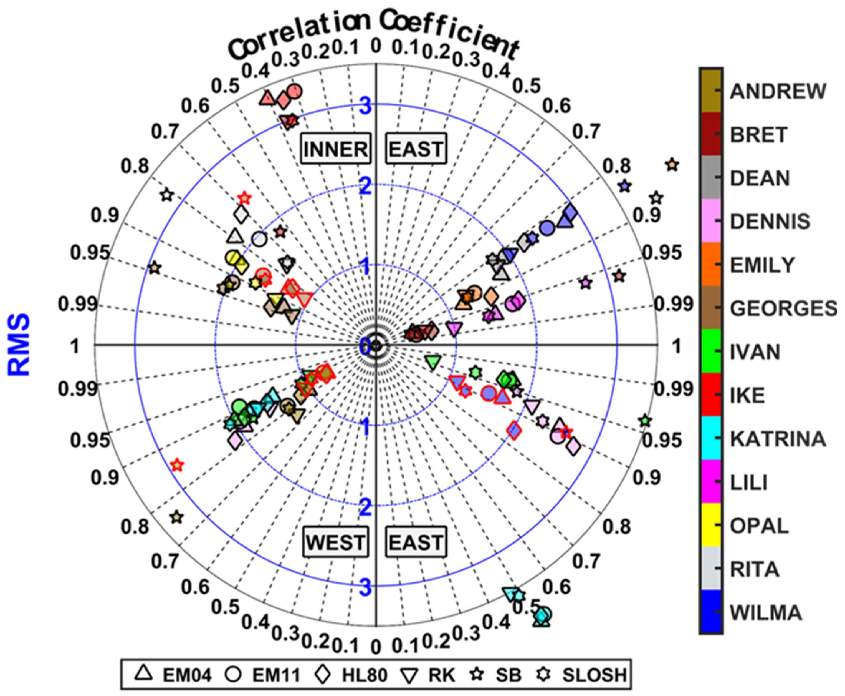
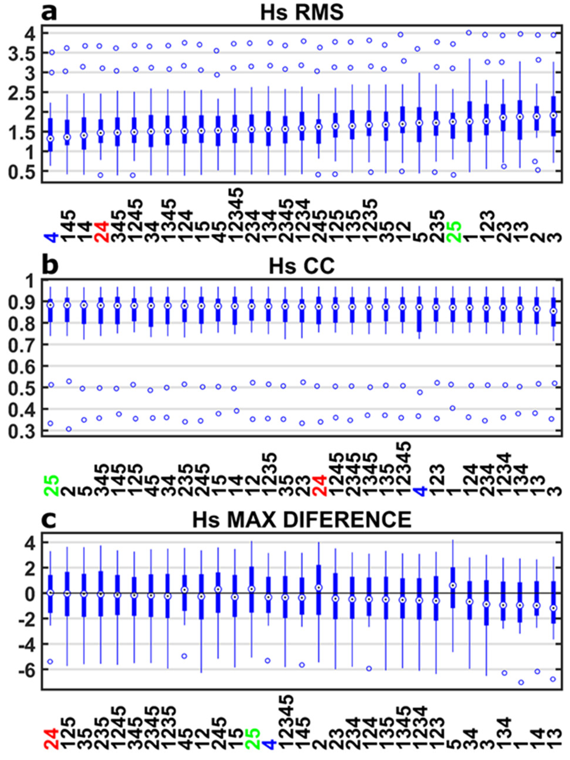
3.2.3. Time Series Permutations

As each model may perform better depending on the TC characteristics (e.g., track and intensity), we hypothesized that using all or some models to calculate the Hs based on an ensemble may provide more accurate results. We then assessed the use of ensembling the results from different models by arranging the resulting time series in all possible combinations, referred to as permutations. Such concept conducts to a resulting wave field which is the average of the wave fields of the models included in each proposed combination of models (each permutation), so the resulting time series correspond to the average of the time series included in each permutation. This means that for each parametric wind field involved in a permutation, we need to run a wave model forced by each parametric wind field. The resulting wave fields are then averaged to obtain a single wave field which is later used to assess its accuracy. Figure 11 shows the assessment of the error measures when comparing the permutations to the same buoy measurements than for the wave assessment, where Figure 11a shows the RMS, Figure 11b the CC and Figure 11c the difference between maximum simulated and measured Hs. Note that we did not consider the SB model for the permutations, as it proved to be an inaccurate model in the previous assessments. The numbers on the x-axis of the figures indicate the models included in each permutation: EM04 (1); EM11 (2); HL80 (3); RK (4); and SLOSH (5).

The results show that some permutations improve the RMS over the use of individual models, except RK, which has the minor RMS median. Nevertheless, the variance may be improved, as shown by the permutation of EM04, RK, and SLOSH models (145 in Figure 11a), which improve the variance in the 75th percentile and 5th percentile for RMS and has a similar median to RK (4 in Figure 11a). Regarding the CC results (Figure 11b), the permutation results are very similar, although RK shows a large variance (4 in Figure 11b). Figure 11c shows the maximum Hs error for all permutation, where permutations 24 and 45 improve Hs maximum differences with similar variance as RK (4). The previous results show that the improvement using permutations is marginal and, in some cases, improving an error measure may worsen another one. However, the permutation approach allows us to quantify uncertainty associated with the use of different parametric models (parameter uncertainty) when conducting wave studies for tropical cyclones. Moreover, while the use of permutations will require an increase number of simulations, the advent of parallel and GPU computing enables the use of permutations as a feasible method to calculate ensemble runs for waves using different parametric wind models.

4. Conclusions

The use of parametric models to determine wind fields to force wave models is a common practice in offshore and coastal engineering. While the use of a particular wind parametric model can be more accurate for a specific event, it is unclear if any specific model is more accurate when simulating a large number of tropical cyclones. As there is a broad suite of parametric wind models, we provide an assessment to determine the accuracy of six commonly used models in engineering practice, focusing on their accuracy when used for wave modeling. As the accuracy of the wave model results depends strongly on the ability of the parametric wind fields to reproduce the TC winds, the accuracy of the HURDAT parameters is crucial. In addition, the inability of the parametric wind models to reproduce strong asymmetries of the wind fields and second eye formations impose limitations on their use for wave modeling.

The results presented show that a particular parametric wind model may more accurately represent the winds for some areas of the TC, or during some stage of its life, but there is not a particular model that overall outperforms the others. The variations in the maximum winds and waves estimates can be up to 15% and 30%, respectively, depending on the parametric model (excluding the SB model, which highly overestimated winds and waves). Concerning the wind fields, EM11 and SLOSH seem to be more accurate to represent areas closer to the eyewall (inner region, from TC center to R_mw), while the central region (from R_mw to 2* R_mw) is better represented by HL80 and RK models, and the outer region (distance from center > 2* R_mw), by RK. In general, the RK model proves to be more accurate when evaluating the results of wave modeling. However, it is a consequence of the slow decaying of the wind profile, which results in the higher waves in areas away from the TC center. As such, the wave error measurements area improved but does not necessarily represent the Hs_max accurately. In general, the wave fields far from the center of the tropical cyclone (distance > 4 R_mw times) will likely not be well represented since there is overall fast wind decay between 2 and 3 R_mw in the parametric wind profiles, particularly in the western areas of the wind field.

The results lead us to conclude that the selection of a particular wind parametric model will be more accurate for some events, but will induce errors for others. Therefore, when modeling a large number of events, we do not expect significant improvements depending on the parametric model used, as the inaccuracy for some events will be compensated with the accuracy of other events. Nevertheless, the SB model proved to result in large overestimations, and, thus, we do not recommend this model in wave studies, unless it is for a particular storm where it proves to be accurate. In addition, the EM04 model is not recommended as it requires the Ro parameter (limiting the TC size), which is usually unavailable for historical storms and synthetic databases. Similarly, EM04, HL80, and RK model depend on the wind profile shape parameters than need be adjusted case by case. Therefore, when modeling a large number of events, we recommend the use of the simplest parametric wind models, without shape parameters, such as EM11 or SLOSH models.

We explored the use of permutations to obtain ensemble results using combinations of different parametric wind models. Results for a limited number of events do not show substantial improvements. However, further research on the implementation of the permutation methods to assess parameter uncertainty, related to the use of different wind parametric models, is warranted.

References

1. Stewart, S.R. Hurricane Ivan: 2–24 September 2004; National Hurricane Center: Miami, FL, USA, 2004; Volume 3.
2. Panchang, V.G.; Li, D. Large waves in the Gulf of Mexico caused by Hurricane Ivan. Bull. Am. Meteorol. Soc. 2006, 87, 481–489. [Google Scholar] [CrossRef]
3. Wang, D.P.; Oey, L.Y. Hindcast of waves and currents in hurricane Katrina. Bull. Am. Meteorol. Soc. 2008, 89, 487–495. [Google Scholar] [CrossRef]
4. Cruz, A.M.; Krausmann, E. Damage to offshore oil and gas facilities following hurricanes Katrina and Rita: An overview. J. Loss Prev. Process Ind. 2008, 21, 620–626. [Google Scholar] [CrossRef]
5. American Petroleum Institute. Interim Guidance on Hurricane Conditions in the Gulf of Mexico; American Petroleum Institute: Washington, DC, USA, 2007. [Google Scholar]
6. Caires, S.; Sterl, A.; Bidlot, J.R.; Graham, N.; Swail, V. Intercomparison of different wind-wave reanalyses. J. Clim. 2004, 17, 1893–1913. [Google Scholar] [CrossRef]
7. Hemer, M.A.; Wang, X.L.; Church, J.A.; Swail, V.R. Coordinating global ocean wave climate projections. Bull. Am. Meteorol. Soc. 2010, 91, 451–454. [Google Scholar] [CrossRef]
8. Jeong, C.K.; Panchang, V.; Demirbilek, Z. Parametric Adjustments to the Rankine Vortex Wind Model for Gulf of Mexico Hurricanes. J. Offshore Mech. Arct. Eng. 2012, 134, 041102. [Google Scholar] [CrossRef]
9. Rotunno, R.; Chen, Y.; Wang, W.; Davis, C.; Dudhia, J.; Holland, G.J. Large-eddy simulation of an idealized tropical cyclone. Bull. Am. Meteorol. Soc. 2009, 90, 1783–1788. [Google Scholar] [CrossRef]
10. Hodges, K.; Cobb, A.; Vidale, P.L. How well are tropical cyclones represented in reanalysis datasets? J. Clim. 2017, 30, 5243–5264. [Google Scholar] [CrossRef]
11. Appendini, C.M.; Torres-Freyermuth, A.; Oropeza, F.; Salles, P.; López, J.; Mendoza, E.T. Wave modeling performance in the Gulf of Mexico and Western Caribbean: Wind reanalyses assessment. Appl. Ocean Res. 2013, 39, 20–30. [Google Scholar] [CrossRef]
12. Wang, X.L.; Swail, V.R. Trends of Atlantic wave extremes as simulated in a 40-yr wave hindcast using kinematically reanalyzed wind fields. J. Clim. 2002, 15, 1020–1035. [Google Scholar] [CrossRef]
13. Knutson, T.R.; Sirutis, J.J.; Garner, S.T.; Held, I.M.; Tuleya, R.E. Simulation of the Recent Multidecadal Increase of Atlantic Hurricane Activity Using an 18-km-Grid Regional Model. Bull. Am. Meteorol. Soc. 2007, 88, 1549–1565. [Google Scholar] [CrossRef] [Green Version]
14. Emanuel, K.; Sundararajan, R.; Williams, J. Hurricanes and global warming: Results from downscaling IPCC AR4 simulations. Bull. Am. Meteorol. Soc. 2008, 89, 347–367. [Google Scholar] [CrossRef]
15. Powell, M.D.; Houston, S.H.; Amat, L.R.; Morisseau-Leroy, N. The HRD real-time hurricane wind analysis system. J. Wind Eng. Ind. Aerodyn. 1998, 77, 53–64. [Google Scholar] [CrossRef]
16. Powell, M.D.; Murillo, S.; Dodge, P.; Uhlhorn, E.; Gamache, J.; Cardone, V.; Cox, A.; Otero, S.; Carrasco, N.; Annane, B.; et al. Reconstruction of Hurricane Katrina’s wind fields for storm surge and wave hindcasting. Ocean Eng. 2010, 37, 26–36. [Google Scholar] [CrossRef]
17. Rankine, W.J.M. A Manual of Applied Physics; Charles Griff and Co.: London, UK, 1882. [Google Scholar]
18. Depperman, C.E. Notes on the origin and structure of Phillipine typhoons. Bull. Am. Meteorol. Soc. 1947, 28, 399–404. [Google Scholar] [CrossRef]
19. Schloemer, R.W. Analysis and Synthesis of Hurricane Wind Patterns over Lake Okeechobee, Florida; Hydrometeorological Reports No. 31; Department of Commerce: Washington, DC, USA, 1954; p. 49.
20. Myers, V.A. Maximum hurricane winds. Bull. Am. Meteorol. Soc. 1957, 38, 227–228. [Google Scholar]
21. Holland, G. An analytic model of the wind and pressure profiles in hurricanes. Mon. Weather Rev. 1980, 108, 1212–1218. [Google Scholar] [CrossRef]
22. Willoughby, H.E.; Rahn, M.E. Parametric Representation of the Primary Hurricane Vortex. Part I: Observations and Evaluation of the Holland (1980) Model. Mon. Weather Rev. 2004, 132, 3033–3048. [Google Scholar] [CrossRef]
23. Holland, G.J.; Belanger, J.I.; Fritz, A. A Revised Model for Radial Profiles of Hurricane Winds. Mon. Weather Rev. 2010, 138, 4393–4401. [Google Scholar] [CrossRef]
24. Vickery, P.J.; Wadhera, D. Statistical models of Holland pressure profile parameter and radius to maximum winds of hurricanes from flight-level pressure and H* wind data. J. Appl. Meteorol. Climatol. 2008, 47, 2497–2517. [Google Scholar] [CrossRef]
25. Thompson, E.F.; Cardone, V.J. Practical Modeling of Hurricane Surface Wind Fields. J. Waterw. Port Coast. Ocean Eng. 1996, 122, 195–205. [Google Scholar] [CrossRef]
26. Vickery, P.J.; Skerlj, P.F.; Steckley, A.C.; Twisdale, L.A. Hurricane wind field model for use in hurricane simulations. J. Struct. Eng. 2000, 126, 1203–1221. [Google Scholar] [CrossRef]
27. Emanuel, K. Tropical cyclone energetics and structure. In Atmospheric Turbulence and Mesoscale Meteorology; Fedorovich, E., Rotunno, R., Stevens, B., Eds.; Cambridge University Press: Cambridge, UK, 2004; pp. 165–192. [Google Scholar] [Green Version]
28. Hu, K.; Chen, Q.; Kimball, S.K. Consistency in hurricane surface wind forecasting: an improved parametric model. Nat. Hazards 2011, 61, 1029–1050. [Google Scholar] [CrossRef]
29. Wood, V.T.; White, L.W.; Willoughby, H.E.; Jorgensen, D.P. A New Parametric Tropical Cyclone Tangential Wind Profile Model. Mon. Weather Rev. 2013, 141, 1884–1909. [Google Scholar] [CrossRef]
30. Chavas, D.R.; Lin, N.; Emanuel, K. A model for the complete radial structure of the tropical cyclone wind field. Part I: Comparison with observed structure. J. Atmos. Sci. 2015, 3647–3662. [Google Scholar] [CrossRef]
31. Phadke, A.C.; Martino, C.D.; Cheung, K.F.; Houston, S.H. Modeling of tropical cyclone winds and waves for emergency management. Ocean Eng. 2003, 30, 553–578. [Google Scholar] [CrossRef]
32. Tolman, H.L.; Alves, J.-H.G.M. Numerical modeling of wind waves generated by tropical cyclones using moving grids. Ocean Model. 2005, 9, 305–323. [Google Scholar] [CrossRef]
33. Peng, M.; Xie, L.; Pietrafesa, L.J. Tropical cyclone induced asymmetry of sea level surge and fall and its presentation in a storm surge model with parametric wind fields. Ocean Model. 2006, 14, 81–101. [Google Scholar] [CrossRef]
34. Lin, N.; Smith, J.A.; Villarini, G.; Marchok, T.P.; Baeck, M.L. Modeling Extreme Rainfall, Winds, and Surge from Hurricane Isabel (2003). Weather Forecast. 2010, 25, 1342–1361. [Google Scholar] [CrossRef]
35. Lin, N.; Chavas, D. On hurricane parametric wind and applications in storm surge modeling. J. Geophys. Res. 2012, 117, D09120. [Google Scholar] [CrossRef]
36. Meza-Padilla, R.; Appendini, C.M.; Pedrozo-Acuña, A. Hurricane-induced waves and storm surge modeling for the Mexican coast. Ocean Dyn. 2015, 65, 1199–1211. [Google Scholar] [CrossRef]
37. Kim, S.Y.; Yasuda, T.; Mase, H. Wave set-up in the storm surge along open coasts during Typhoon Anita. Coast. Eng. 2010, 57, 631–642. [Google Scholar] [CrossRef]
38. Lin, N.; Emanuel, K.A.; Smith, J.A.; Vanmarcke, E. Risk assessment of hurricane storm surge for New York City. J. Geophys. Res. 2010, 115, D18121. [Google Scholar] [CrossRef]
39. Lin, N.; Lane, P.; Emanuel, K.A.; Sullivan, R.M.; Donnelly, J.P. Heightened hurricane surge risk in northwest Florida revealed from climatological-hydrodynamic modeling and paleorecord reconstruction. J. Geophys. Res. Atmos. 2014, 119, 8606–8623. [Google Scholar] [CrossRef]
40. Rey, W.; Mendoza, T.E.; Salles, P.; Zhang, K.; Teng, Y.; Miguel, A.; Franklin, G.L. Hurricane Flood Risk Assessment for the Yucatan and Campeche State Coastal Area. Nat. Hazards 2019, 96, 1041–1065. [Google Scholar] [CrossRef]
41. Mattocks, C.; Forbes, C. A real-time, event-triggered storm surge forecasting system for the state of North Carolina. Ocean Model. 2008, 25, 95–119. [Google Scholar] [CrossRef]
42. Appendini, C.M.; Rosengaus, M.; Meza-Padilla, R.; Camacho-Magaña, V. Operational hazard assessment of waves and storm surges from tropical cyclones in Mexico. Bull. Am. Meteorol. Soc. 2017, 98, 503–515. [Google Scholar] [CrossRef]
43. Appendini, C.M.; Torres-Freyermuth, A.; Salles, P.; López-González, J.; Mendoza, E.T. Wave climate and trends for the Gulf of Mexico: A 30-yr wave hindcast. J. Clim. 2014, 27, 1619–1632. [Google Scholar] [CrossRef]
44. Vickery, P.J.; Wadhera, D.; Galsworthy, J.; Peterka, J.A.; Irwin, P.A.; Griffis, L.A. Ultimate Wind Load Design Gust Wind Speeds in the United States for Use in ASCE-7. J. Struct. Eng. 2009, 136, 613–625. [Google Scholar] [CrossRef]
45. Appendini, C.M.; Pedrozo-Acuña, A.; Meza-Padilla, R.; Torres-Freyermuth, A.; Cerezo-Mota, R.; López-González, J.; Ruiz-Salcines, P. On the Role of Climate Change on Wind Waves Generated by Tropical Cyclones in the Gulf of Mexico. Coast. Eng. J. 2017, 59, 32. [Google Scholar] [CrossRef]
46. Panchang, V.; Kwon Jeong, C.; Demirbilek, Z. Analyses of Extreme Wave Heights in the Gulf of Mexico for Offshore Engineering Applications. J. Offshore Mech. Arct. Eng. 2013, 135, 031104. [Google Scholar] [CrossRef]
47. Krien, Y.; Arnaud, G.; Cécé, R.; Khan, J.; Madani, A.B.; Bernard, D.; Islam, A.K.M.S.; Durand, F.; Testut, L.; Palany, P.; et al. Can We Improve Parametric CyclonicWind Fields Using Recent Satellite Remote Sensing Data? Remote Sens. 2018, 10, 1963. [Google Scholar] [CrossRef]
48. Landsea, C.W.; Franklin, J.L. Atlantic Hurricane Database Uncertainty and Presentation of a New Database Format. Mon. Weather Rev. 2013, 141, 3576–3592. [Google Scholar] [CrossRef]
49. Silva, R.; Govare, G.; Salles, P.; Bautista, G.; Diaz, G. Oceanographic Vulnerability to Hurricanes on the Mexican Coast. Costal Eng. Conf. 2002, 1, 39–51. [Google Scholar]
50. Knaff, J.A.; Sampson, C.R.; DeMaria, M.; Marchok, T.P.; Gross, J.M.; McAdie, C.J. Statistical Tropical Cyclone Wind Radii Prediction Using Climatology and Persistence. Weather Forecast. 2007, 22, 781–791. [Google Scholar] [CrossRef]
51. Takagi, H.; Wu, W. Maximum wind radius estimated by the 50 kt radius: Improvement of storm surge forecasting over the western North Pacific. Nat. Hazards Earth Syst. Sci. 2016, 16, 705–717. [Google Scholar] [CrossRef]
52. Jarvinen, B.R.; Neumann, C.J.; Davis, M.A.S. A Tropical Cyclone Data Tape for The North Atlantic Basin, 1886–1983: Contents, Limitations, and Uses; NOAA Technical Memorandum NWS NHC 22, NOAA/Tropical Prediction Center; National Oceanic and Atmospheric Administration: Miami, FL, USA, 1984.
53. Dinapoli, S.M.; Bourassa, M.A.; Powell, M.D. Uncertainty and Intercalibration Analysis of H*Wind. J. Atmos. Ocean. Technol. 2012, 29, 822–833. [Google Scholar] [CrossRef]
54. Mears, C.A.; Smith, D.K.; Wentz, F.J. Comparison of Special Sensor Microwave Imager and buoy-measured wind speeds from 1987 to 1997. J. Geophys. Res. 2001, 106, 11719. [Google Scholar] [CrossRef]
55. Riehl, H. Some relationships between wind and thermal structure of steady state hurricanes. J. Atmos. Sci. 1963, 20, 276–287. [Google Scholar] [CrossRef]
56. Emanuel, K.A. An Air-Sea Interaction Theory for Tropical Cyclones. Part I: Steady-State Maintenance. J. Atmos. Sci. 1986, 43, 585–605. [Google Scholar] [CrossRef]
57. Cao, Y.; Fovell, R.G.; Corbosiero, K.L. Tropical cyclone track and structure sensitivity to initialization in idealized simulations: A preliminary study. Terr. Atmos. Ocean. Sci. 2011, 22, 559–578. [Google Scholar] [CrossRef]
58. Mallen, K.J.; Montgomery, M.T.; Wang, B. Reexamining the Near-Core Radial Structure of the Tropical Cyclone Primary Circulation: Implications for Vortex Resiliency. J. Atmos. Sci. 2005, 62, 408–425. [Google Scholar] [CrossRef] [Green Version]
59. Levinson, D.H.; Vickery, P.J.; Resio, D.T. A review of the climatological characteristics of landfalling Gulf hurricanes for wind, wave, and surge hazard estimation. Ocean Eng. 2010, 37, 13–25. [Google Scholar] [CrossRef]
60. Young, I.; Sobey, R. The Numerical Prediction of Tropical Cyclone Wind-Waves; Department of Civil & Systems Engineering, James Cook University of North Queensland: Townsville, Australia, 1981. [Google Scholar]
61. Jelesnianski, C.P.C. Numerical computations o f storm surges without bottom stress. Mon. Weather Rev. 1966, 94, 379–394. [Google Scholar] [CrossRef]
62. Houston, S.H.; Powell, M.D. Observed and Modeled Wind and Water-Level Response from Tropical Storm Marco (1990). Weather Forecast. 1994, 9, 427–439. [Google Scholar] [CrossRef] [Green Version]
63. Houston, S.H.; Shaffer, W.A.; Powell, M.D.; Chen, J. Comparisons of HRD and SLOSH Surface Wind Fields in Hurricanes: Implications for Storm Surge Modeling. Weather Forecast. 1999, 14, 671–686. [Google Scholar] [CrossRef] [Green Version]
64. Emanuel, K.; Ravela, S.; Vivant, E.; Risi, C. A statistical deterministic approach to hurricane risk assessment. Bull. Am. Meteorol. Soc. 2006, 87, 299–314. [Google Scholar] [CrossRef]
65. Chavas, D.R.; Emanuel, K.A. A QuikSCAT climatology of tropical cyclone size. Geophys. Res. Lett. 2010, 37, 10–13. [Google Scholar] [CrossRef]
66. Emanuel, K.; Ravela, S. Synthetic Storm Simulation for Wind Risk Assessment. In Storm Surge Barriers to Protect New York City Against The Deluge; American Society of Civil Engineers: Reston, VA, USA, 2012; pp. 15–36. ISBN 978-0-7844-1252-7. [Google Scholar]
67. Emanuel, K.; Rotunno, R. Self-Stratification of Tropical Cyclone Outflow. Part I: Implications for Storm Structure. J. Atmos. Sci. 2011, 68, 2236–2249. [Google Scholar] [CrossRef]
68. Chan, J.C.L.L. the Physics of Tropical Cyclone Motion. Annu. Rev. Fluid Mech. 2005, 37, 99–128. [Google Scholar] [CrossRef]
69. Lin, N.; Emanuel, K.; Oppenheimer, M.; Vanmarcke, E. Physically based assessment of hurricane surge threat under climate change. Nat. Clim. Chang. 2012, 2, 462–467. [Google Scholar] [CrossRef] [Green Version]
70. Powell, M.D.; Houston, S.H. Hurricane Andrew’s Landfall in South Florida. Part II: Surface Wind Fields and Potential Real-Time Applications. Weather Forecast. 1996, 11, 329–349. [Google Scholar] [CrossRef]
71. Dunion, J.P.; Landsea, C.W.; Houston, S.H.; Powell, M.D. A Reanalysis of the Surface Winds for Hurricane Donna of 1960. Mon. Weather Rev. 2003, 131, 1992–2011. [Google Scholar] [CrossRef] [Green Version]
72. Vickery, P.J.; Wadhera, D.; Powell, M.D.; Chen, Y. A Hurricane Boundary Layer and Wind Field Model for Use in Engineering Applications. J. Appl. Meteorol. Climatol. 2009, 48, 381–405. [Google Scholar] [CrossRef]
73. Kepert, J.D. Slab-and height-resolving models of the tropical cyclone boundary layer. Part I: Comparing the simulations. Q. J. R. Meteorol. Soc. 2010, 136, 1686–1699. [Google Scholar] [CrossRef]
74. Bretschneider, C.L. A Non-Dimensional Stationary Hurricane Wave Model. In Proceedings of the Offshore Technology Conference; Offshore Technology Conference, Houston, TX, USA, 1–3 May 1972. [Google Scholar]
75. Vickery, P.J.; Masters, F.J.; Powell, M.D.; Wadhera, D. Hurricane hazard modeling: The past, present, and future. J. Wind Eng. Ind. Aerodyn. 2009, 97, 392–405. [Google Scholar] [CrossRef]
76. Harper, B.; Holland, G. An updated parametric model of the tropical cyclone. In Proceedings of the 23rd Conference Hurricanes and Tropical Meteorology, Dallas, TX, USA, 10–15 January 1999; pp. 10–15. [Google Scholar]
77. Powell, M.D. Evaluations of Diagnostic Marine Boundary-Layer Models Applied to Hurricanes. Mon. Weather Rev. 1980, 108, 757–766. [Google Scholar] [CrossRef] [Green Version]
78. Powell, M.D. An analytic model of the wind and pressure profiles in hurricanes. Mon. Weather Rev. 1987, 115, 75–89. [Google Scholar] [CrossRef]
79. Powell, M.D.; Black, P.G. The relationship of hurricane reconnaissance flight-level wind measurements to winds measured by NOAA’s oceanic platforms. J. Wind Eng. Ind. Aerodyn. 1990, 36 Pt 1, 381–392. [Google Scholar] [CrossRef]
80. Georgicu, P.N.; Davenport, A.G.; Vickery, B.J. Design windspeeds in regions dominated by tropical cyclones. J. Wind Eng. Ind. Aerodyn. 1983, 13, 139–152. [Google Scholar] [CrossRef]
81. Batts, M.E.; Cordes, M.R.; Russell, L.R.; Shaveri, J.R.; Simiu, E. Hurricane Wind Speeds in the United States; U.S. Department of Commerce: Washington, DC, USA; National Bureau of Standards: Gaithersburg, MD, USA, 1984.
82. Willoughby, H.E.; Clos, J.A.; Shoreibah, M.G.; Willoughby, H.E.; Clos, J.A.; Shoreibah, M.G. Concentric Eye Walls, Secondary Wind Maxima, and The Evolution of the Hurricane vortex. J. Atmos. Sci. 1982, 39, 395–411. [Google Scholar] [CrossRef]
83. Sørensen, O.R.; Kofoed-Hansen, H.; Rugbjerg, M.; Sørensen, L.S. A third-generation spectral wave model using an unstructured finite volume technique. In Proceedings of the 29th International Conference on Coastal Engineering, Lisbon, Portugal, 19–24 September 2004; pp. 894–906. [Google Scholar]
84. Ruiz-Salcines, P. Campos de Viento Para HIndcast de Oleaje: Reanálisis, Paramétricos y Fusión; Universidad de Cantabria: Santander, Cantabria, 2013. [Google Scholar]
85. Tolman, H.L. Alleviating the Garden Sprinkler Effect in wind wave models. Ocean Model. 2002, 4, 269–289. [Google Scholar] [CrossRef]
86. Amante, C.; Eakins, B.W. ETOPO1 1 Arc-Minute Global Relief Model: Procedures, Data Sources and Analysis; NOAA Technical Memorandum NESDIS NGDC-24; National Geophysical Data Center: Boulder, CO, USA; Marine Geology and Geophysics Division: Boulder, CO, USA, 2009; p. 19.
87. DeMaria, M. The Effect of Vertical Shear on Tropical Cyclone Intensity change. J. Atmos. Sci. 1996, 53, 2076–2087. [Google Scholar] [CrossRef]
88. Wang, Y.; Holland, G.J. Tropical cyclone motion and evolution in vertical shear. J. Atmos. Sci. 1996, 53, 3313–3332. [Google Scholar] [CrossRef]
89. Bender, M.A. The Effect of Relative Flow on the Asymmetric Structure in the Interior of Hurricanes. J. Atmos. Sci. 1997, 54, 703–724. [Google Scholar] [CrossRef] [Green Version]
90. Frank, W.M.; Ritchie, E.A. Effects of Vertical Wind Shear on the Intensity and Structure of Numerically Simulated Hurricanes. Mon. Weather Rev. 2001, 129, 2249–2269. [Google Scholar] [CrossRef]
91. Shay, L.K.; Goni, G.J.; Black, P.G. Effects of a Warm Oceanic Feature on Hurricane Opal. Mon. Weather Rev. 2000, 128, 1366–1383. [Google Scholar] [CrossRef]
92. Powell, M.D.; Houston, S.H. Surface wind fields of 1995 Hurricanes Erin, Opal, Luis, Marilyn, and Roxanne at landfall. Mon. Weather Rev. 1998, 126, 1259–1273. [Google Scholar] [CrossRef]
93. Houze, R.A.; Chen, S.S.; Smull, B.F.; Lee, W.C.; Bell, M.M. Hurricane intensity and eyewall replacement. Science 2007, 315, 1235–1239. [Google Scholar] [CrossRef]
Figure 1. Buoy locations (colored triangles) and 1-h cubic spline interpolated tropical cyclone trajectories and category (colored lines). The number denotes the tropical cyclone as follows: (1) Andrew 1992; (2) Opal 1995; (3) Georges 1998; (4) Bret 1999; (5) Lili 2002; (6) Ivan 2004; (7) Dennis 2005; (8) Emily 2005; (9) Katrina 2005; (10) Rita 2005; (11) Wilma 2005; (12) Dean 2007; and (13) Ike 2008.
Water 11 02044 g001
Figure 2. Comparison of normalized wind profiles for different parametric models: (a) Katrina on 26 August 2005 at 12:00 UTC (Category 1) with Vmax = 38.58 m/s, ΔP = 32 mb, Rmw = 37.04 km, latitude = 25.1°; and (b) Rita on 22 September 2005 at 6:00 UTC (Category 5) with Vmax = 56.59 m/s, ΔP = 113 mb, Rmw = 37.04 km, latitude = 24.8°. Ro = 1000 km is considered in both cases. Blue dashed line shows the position of r = 150 km.
Water 11 02044 g002
Figure 3. Subset of radial wind profiles as a function of normalized distance by r/Rmw from H*Wind and parametric models, for TC in categories 1–5, at 45°, 90°, 135° and 180° taken as reference the track direction. Subplot title includes TC name and date (month, day, hour, and minute).
Water 11 02044 g003
Figure 4. Radial wind profiles mean r2 for tropical storm (TT), categories 1 and 2, and categories 3–5 for all models.
Water 11 02044 g004
Figure 5. Root-mean-square error (RMS) and correlation coefficient (CC) boxplot wind speed comparison between time series of H*Wind and parametric models (a,b in top panels) and at normalized locations (each 22.5° clockwise from HURDAT2 TC trajectory and at different distances from the storm center, 0.3, 0.7, 1, 1.5, 2, 2.5, 3 and 4 *Rmw in each time step) for all (ALL) (c,f), right (RIGHT) (d,g), and left (LEFT) (e,h) quadrants. Time series represents all the time steps with H*Wind data. Each box represents the 25th percentile (bottom) and 75th percentile (top) bounding the median (middle line), the wider dash lines represent the 10th percentile (bottom) and 90th percentile (top), and red points represent above 90th percentile.
Water 11 02044 g005
Figure 6. H*Wind and parametric steady-state wind and significant wave heights (Hs) fields associated for static situation corresponding to Dean as category 1 at 20070822T0730 (left panels) and Rita as category 5 at 20050922T1330 (right panels). Circles correspond to the distance of Rmw and 2 × Rmw. The black arrow shows the TC direction.
Water 11 02044 g006
Figure 7. Significant wave height (Hs) time series measured from NDBC buoys and estimated from the parametric models, for the selected tropical cyclones. Data in each figure: upper left corner: the angle between track and buoy (in degrees from TC translation direction to buoy and positive clockwise); right upper corner category; distance (as a function of Rmw) from the TC center to the buoy in the nearest time step. The subplots are grouped in columns according to the buoy location related to the TC center (the inner region, when the buoy is inside areas minor than Rmw and east and west buoy’s position respect the translation direction of the TC). The x-axis shows the date of the time series in day/hour format (DD/HH).
Water 11 02044 g007
Figure 8. Circular diagram of root mean square error (RMS) (blue concentric circles) and correlation coefficient (CC) (radial black dotted lines) calculated from the resulting Hs covering 24 h before and after the TC crosses a particular buoy (shown by different symbols). The results are grouped in different quadrants according to the location of the buoy relative to the TC center (inner region when the buoy is located at less than one Rmw, and east and west depending on the buoy position with respect the translation direction of the TC). The events corresponding to Georges for buoy 42040 (inner region), Wilma for buoy 42057 (east) and Andrew for buoy 42001 (west) are represented with a red edge color to differentiate them at the buoys 42003, 42056 and 42003 respectively (black edge color). The SB model results for Katrina in buoy 42001 and Emily in buoy 42056 do not appear as they have very high RMS values and are outside the plot limits (RMS = 4.52; 4.31 and CC = 0.89; 0.85 respectively).
Water 11 02044 g008
Figure 9. Maximum Hs error percentage between model results and measurements for all TC.
Water 11 02044 g009
Figure 10. Boxplots of: (ad) maximum Hs percent error between buoys and model results; (eh) corresponding root-mean-square error; and (il) correlation coefficient. Boxplots of: (a,e,i) all areas; (b,f,j) the inner region (buoy located at a distance less than the Rmw from the TC); (c,g,k) the east; and (d,h,l) the west, referring to the buoy location relative to the TC center considering the translation direction of the TC.
Water 11 02044 g010
Figure 11. Significant wave height: (a) root-mean-square error; (b) correlation coefficient; and (c) difference between maximum simulated and measured. The numbers in the x-axis indicate the models included in each permutation: (1) EM04; (2) EM11; (3) HL80; (4) RK; and (5) SLOSH. The error measures are calculated from the time series selected by 24 h before and after the TC crosses the buoys. Each box represents the 25th percentile (bottom) and 75th percentile (top), the median is the blue circle with a black point inside, the blue lines represent the 10th percentile (bottom) and 90th percentile (top), blue circles points represent above and below 90th percentile and 10th percentile. The error measures are ordered from less to more error denoting the results in blue RMS, green for CC, and red for the maximum difference.
Water 11 02044 g011