Stochastic Model for Drought Forecasting in the Southern Taiwan Basin

Abstract

The global rainfall pattern has changed because of climate change, leading to numerous natural hazards, such as drought. Because drought events have led to many disasters globally, it is necessary to create an early warning system. Drought forecasting is an important step toward developing such a system. In this study, we utilized the stochastic, autoregressive integrated moving average (ARIMA) model to predict drought conditions based on the standardized precipitation index (SPI) in southern Taiwan. We employed data from 1967 to 2006 to train the model and data from 2007 to 2017 for model validation. The results showed that the coefficients of determination (R²) were over 0.80 at each station, and the root-mean-square error and mean absolute error were sufficiently low, indicating that the ARIMA model is effective and adequate for our stations. Finally, we employed the ARIMA model to forecast future drought conditions from 2019 to 2022. The results yielded relatively low SPI values in southern Taiwan in future summers. In summary, we successfully constructed an ARIMA model to forecast drought. The information in this study can act as a reference for water resource management.

1. Introduction

Drought is a natural phenomenon which can be classified into four categories: meteorological, hydrological, agricultural, and socioeconomic drought. Among these, meteorological drought can precede and lead to the other three types. It is essentially caused by insufficient precipitation and usually results in severe disaster events. Dai [1] found that the global trends of observed annual precipitation from 1950 to 2010 showed a decline in areas such as Africa, Southeast and East Asia, Eastern Australia, and Southern Europe. These results indicate that water shortages are becoming increasingly severe, which may lead to drought. However, drought events not only lead to environmental changes but also have serious impacts on the social economy and agricultural development [2]. For example, between 1976 and 2006, the total cost associated with drought in Europe was as high as €100 billion, while the number of people affected by drought increased by 20% [3]. Therefore, it is important to assess drought conditions to develop a mitigation strategy.

Many drought indices have been proposed to assess meteorological drought to identify the occurrence of drought events. Among these, the standardized precipitation index (SPI) has been widely employed to evaluate the intensity of meteorological droughts, owing to the following advantages. First, the SPI is based only on long-term rainfall data. Second, the SPI is in a standardized form, which means that it can be compared between different regions. Third, it has variable timescales, which allows it to describe different drought conditions. Therefore, the SPI was selected as the meteorological drought index in the present study.

Because a drought varies slowly in time, it is generally not discovered until a disaster occurs. Therefore, an effective monitoring system is required to mitigate the impacts of droughts. An effective monitoring system can help to establish an early warning system for drought [4], and drought forecasting is an important step toward developing such an early warning system. Forecasting future drought conditions in a region is critical for the sustainability of water resource planning and management. In addition, drought forecasting plays a vital role in drought risk assessment [5,6] and provides information for water resource managers and policy makers to take precautions against droughts in advance [7]. There have been many previous studies concerning drought forecasting, such as detecting occurrences of drought and predicting the duration and severity of a drought event. However, the main challenge is to select a suitable and effective tool for forecasting [6,7,8].

There exist many methodologies for forecasting drought events based on drought indices, such as regression analysis [9,10], stochastic models [7,11,12,13,14], probability models [15], artificial intelligence (AI)-based models [16,17,18,19], and dynamic modeling [20,21].

The stochastic model, also known as the time series model, has been utilized to predict hydrological time series. In general, the time series model has a weak capability for modeling data with nonlinear characteristics but is able to effectively fit linear data such as streamflow and precipitation. In addition, there are periodic characteristics and serial correlations between observations in hydrological time series, and the time series model can describe these features well and perform systematic modeling. The most useful and common class of stochastic model is the autoregressive integrated moving average (ARIMA) model. The advantages of the ARIMA model include low data input requirements, a simple computational process [22], and few model parameters being required to describing the time series [10,11]. It is also suitable for nonstationary data. Owing to these merits, this time series model is superior to other statistical models [7,23].

The purpose of this study was to develop a valid linear stochastic model based on an SPI time series in southern Taiwan. According to a previous study, most studies have only developed the ARIMA model to fit their own time series data, and few studies have actually predicted future drought situations. Hence, in this study, we utilized the ARIMA model to forecast drought conditions over next four years, from 2019 to 2022.

2. Study Area

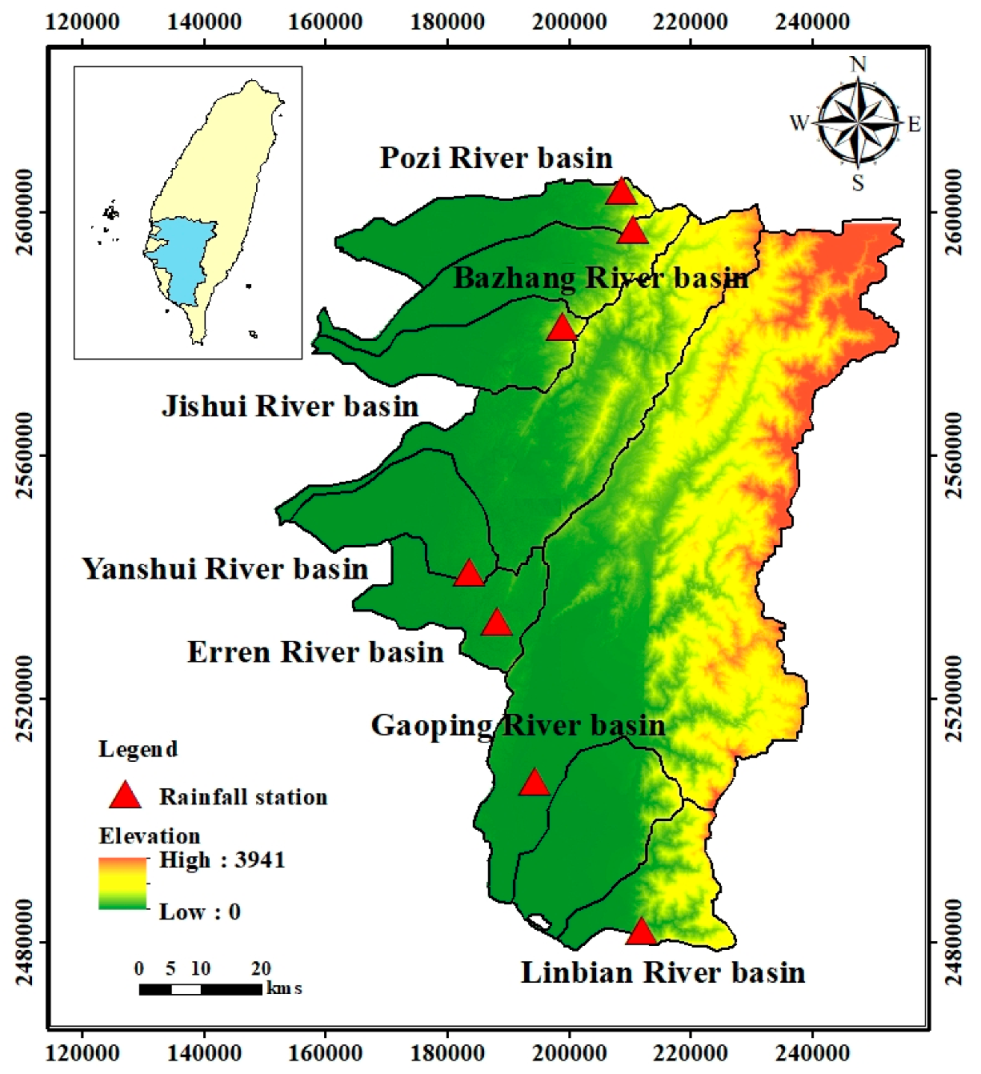
The study area is located in southern Taiwan and includes the Pozi River basin, Bazhang River basin, Jishui River basin, Yanshui River basin, Erren River basin, Gaopping River basin, and Linbian River basin. It belongs to the tropical monsoon climate zone. There is abundant rainfall, but owing to the uneven distribution of rainfall in time and space, the region is characterized by distinct wet and dry seasons. In this study, we selected one rainfall station in each basin, with records from the years 1967 to 2017. Information on the rainfall stations is presented in

Table 1. Information on rainfall stations at each basin.

Basin	Station	Short Name
Pozi River basin	Zhang Nao Liao-2	PR1
Bazhang River basin	Da Hu Shan	BR1
Jishui River basin	Guan Zi Ling-2	GR1
Yanshui River basin	Qi Ding	YR2
Erren River basin	Gu Ting Keng	RR2
Gaoping River basin	Ping Dong-5	KR3
Linbian River basin	Nan Han	LR2

, and the spatial distributions of the rainfall stations at each basin are shown in Figure 1.

3. Methodology

3.1. SPI

There exist many methods that can identify drought events, and using drought indicators is the most convenient and effective method to do this. In this study, we explored meteorological drought in southern Taiwan. The SPI was proposed by McKee et al. [24]. This index simply utilizes the cumulative precipitation data over different periods for calculation. Because the index is standardized, it can be compared between different regions. The World Meteorological Organization [25] listed this as the preferred index for describing precipitation drought events. Considering the rainfall pattern in Taiwan, over a shorter aggregation time scale, the SPI only exhibits periodic oscillations in time, and it is difficult to evaluate long-term drought events. In contrast, it is easier to identify drought events with a longer aggregation time scale. Therefore, we chose a 12 month aggregation time scale for the SPI. In this study, we utilized historical SPI time series to predict future drought conditions using a time series model.

3.2. Time Series Model

The time series model is a stochastic model that is commonly used for time series forecasting. Common time series models include the autoregressive (AR), moving average (MA), and autoregressive moving average (ARMA) models. Many studies have employed time series models to predict hydrological and meteorological time series [7,11,26].

3.2.1. Nonseasonal ARIMA Model

The AR and MA models can be effectively combined into an ARMA model. The current data is analyzed by a linear combination of previous data plus error terms. However, the ARMA model is only applicable when the data is stationary. If the original time series is nonstationary, then the difference must be added. The resulting model is called the ARIMA model, as proposed by Box and Jenkins [27]. The ARIMA model provides a new generation of forecasting tools, emphasizing the stochastic properties of time series rather than constructing single and simultaneous equation models. Each variable of the ARIMA model is represented by its own lagged value and stochastic error terms. The general nonseasonal ARIMA model consists of a p-order AR model, a q-order MA model, and the operators on the dth difference of the original time series data. This can be expressed as ARIMA(p,d,q), and the algorithm of the model is as follows:

$$\varphi (L){\nabla }^d{x}_t=\theta (L){\epsilon }_t$$

(1)

where $\varphi (L)$ and $\theta (L)$ are polynomials of order p and q, respectively. The operators for the nonseasonal AR model of order p and MA model of order q are written as

$$\begin{array}{l}\varphi (L)=(1-{\varphi }_{1}L-{\varphi }_2{L}^2-\cdots -{\varphi }_p{L}^p)\\ \theta (L)=(1-{\theta }_{1}L-{\theta }_2{L}^2-\cdots -{\theta }_p{L}^p)\end{array}$$

(2)

where L is the lag operator $L^i{x}_t=x_{t-i}$.

3.2.2. Seasonal ARIMA (SARIMA) Model

Box et al. [28] extended the ARIMA model to deal with seasonality, with the result commonly referred to as the SARIMA model. The SARIMA model is analyzed by introducing seasonal periodic change to a general ARIMA mode, and it can be denoted as ARIMA(p,d,q)(P,D,Q)_S, where (p,d,q) is the nonseasonal part of the model and (P,D,Q)_S is the seasonal part. This can be expressed as follows:

$${\varphi }_p(L){\Phi }_P(L^s){\nabla }^d{\nabla }_s^D{x}_t={\theta }_q(L^s){\Theta }_Q(L^s){\epsilon }_t$$

(3)

where p is the order of the nonseasonal AR model, q is the order of the nonseasonal MA model, d is the order of the general difference, P is the order of the seasonal AR model, Q is the order of the seasonal MA model, D is the seasonal differencing, and S is the length of a season.

3.3. ARIMA Model Development

In general, the development and selection of an appropriate ARIMA model consists of three steps: model identification, parameter estimation, and diagnostic checking [23,27,29,30].

3.3.1. Model Identification

This step involves transforming the data which is to confirm the original data to normality and stationarity and utilizing the autocorrelation function (ACF) and partial autocorrelation function (PACF) to initially confirm the general form of the ARIMA model. Here, the ACF and PACF were used to determine the order of the model, and the final model was selected using the goodness-of-fit criteria through the Akaike information criterion (AIC) [31] and Schwarz–Bayesian criterion (SBC) [32]. The model that gives the minimum AIC and SBC value is selected as the best. The mathematical formulations of the AIC and SBC are as follows:

$$\mathrm{AIC}=n\ln (MSE)+2m$$

(4)

$$\mathrm{SBC}=n\ln (MSE)+m\ln (n)$$

(5)

where $m=(p+q+P+Q)$ is the number of model parameters, n is the number of data, and MSE is the mean-square error.

$$\mathrm{Mean}\mathrm{square}\mathrm{error}(MSE)=\frac{1}{n}{\displaystyle \sum _{i=1}^n{(y_t-{\widehat{y}}_t)}^2}$$

(6)

where y_t is the observed data and ${\widehat{y}}_t$ is the predicted value.

3.3.2. Parameter Estimation

After identifying the ARIMA model, the parameters of the model must be estimated. This study employed the method of maximum likelihood, as proposed by Box and Jenkins [27], to estimate the parameters of the ARIMA model. Maximum likelihood estimation is a method of estimating the parameters of a statistical model.

3.3.3. Diagnostic Checking

Once an appropriate model has been selected and the parameters have been estimated, diagnosing the ARIMA model represents a crucial component of model development. In this step, it is necessary to verify whether the residuals of the model satisfy the properties of independence, following a normal distribution, and homoscedasticity to verify that the model is suitable for time series. Several statistical tests and plots of residuals are utilized for diagnostic checking. For a good model, the residuals must satisfy the white noise process requirements of being uncorrelated and normally distributed around a zero mean.

The residual autocorrelation function (RACF) and residual partial autocorrelation function (RPACF) of a time series are utilized to determine whether the series is independent. If the ACF and PACF of the residuals are significant within the confidence limits, this indicates that there is no significant correlation between the residuals. An alternative method is the Ljung–Box–Pierce (LBQ) test, which is a statistical method of testing for residual autocorrelation. The null hypothesis of the LBQ test is that the residuals are independent. The test statistic is defined in Equation (7):

$$Q=n(\mathrm{n}+2){\displaystyle \sum _{k=1}^m\frac{r_k^2}{n-k}}$$

(7)

where m is the number of autocorrelation lags, n is the number of data, and r_k is the sample autocorrelation at lag k. The statistical Q values are compared with the critical value with the degree of freedom at a 5% significance level. If the calculated values are less than the critical value, this means the residuals of the model are in accordance with white noise.

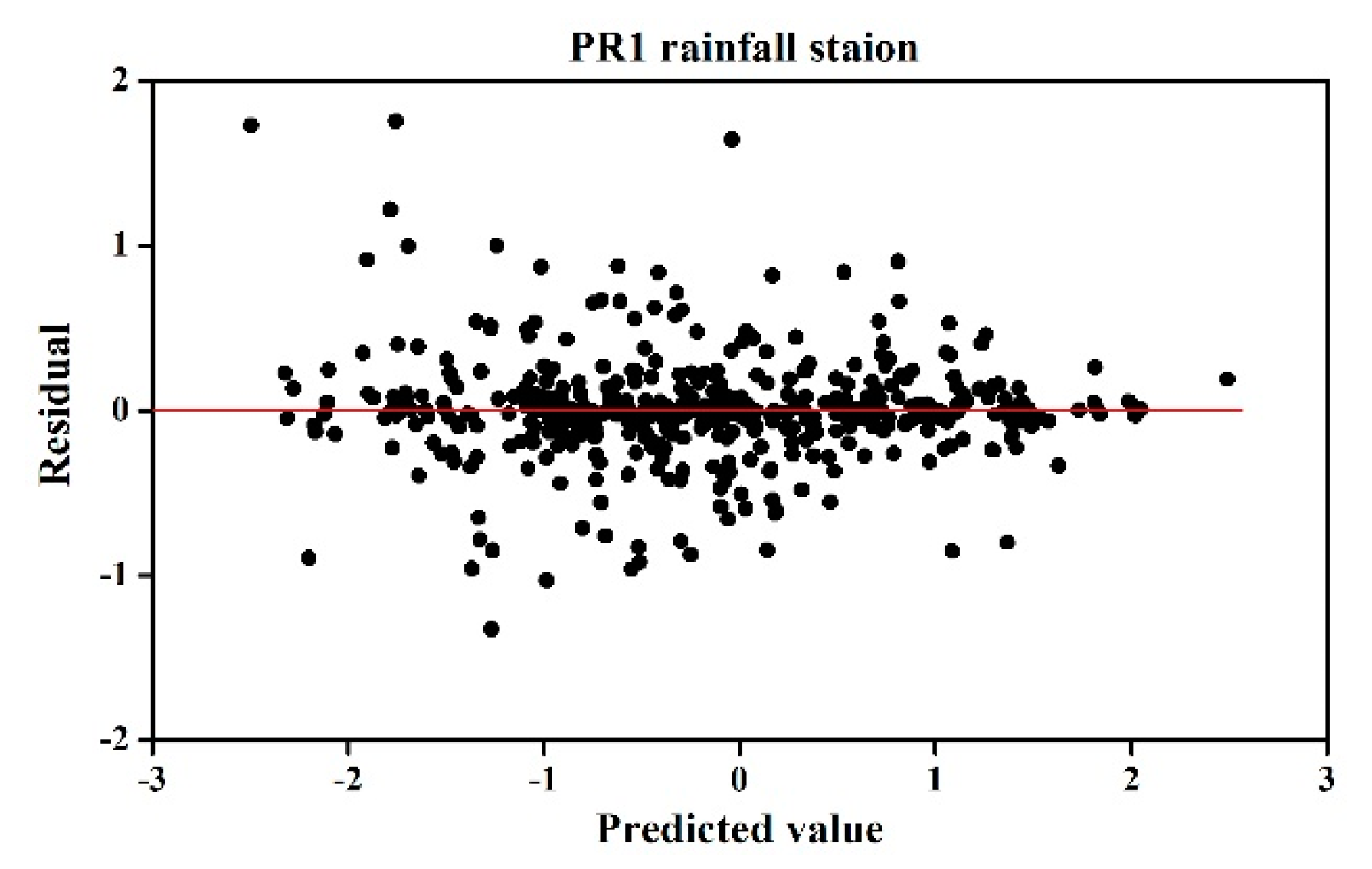
The normality of residuals is verified by histograms and a probability plot of residuals. The residuals are also verified for homoscedasticity, which means there is a constant error variance over all the data. This is verified through a scatterplot of the residuals against predicted values. If the scatterplot exhibits no obvious patterns and the residuals are distributed randomly around zero, this indicates the residuals are homoscedastic.

4. Results and Discussion

In this study, to perform the predictive analysis, we selected seven stations with long-term monitoring data in the study area. The dataset was divided into two periods: training data (from 1967 to 2006) and validation data (from 2007 to 2017). Here, we used the ARIMA model to forecast future drought conditions based on the SPI. The model development steps included model identification, parameter estimation, and diagnostic checking. In this study, we utilized MATLAB to develop the time series model.

4.1. Model Identification

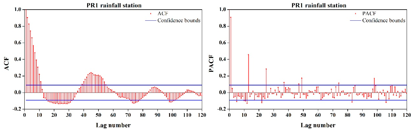
There are two main stages in model identification: (1) confirm whether the data is stationary and (2) utilize the ACF and PACF to determine the general form of the ARIMA model. According to the Kwiatkowski, Phillips, Schmidt, and Shin (KPSS) test, our data was nonstationary, and so it needed to be differenced. After applying the first-order difference, each station satisfied the model development conditions. Because the data at every station exhibited a similar pattern, we simply took the PR1 station as an example. Figure 2 shows that the ACF curve was damping out in a sine wave and the PACF exhibited a significant spike at lag 1, which reflected the AR(1) process. In addition, there were significant spikes in the PACF at lags 12, 24, 36, and 48, which indicated that the data exhibited seasonality with a period of 12. In the ACF, each station had a sine wave pattern, which also indicated that the data was seasonal [13]. Therefore, we chose AR(1) as the nonseasonal part of the ARIMA model, and the peaks at the lags that were multiples of 12 in the PACF indicated a seasonal model, which comprised the SARIMA model. The AIC and SBC criteria were utilized to select the best model, and the results are shown in

Table 2. The Akaike information criterion (AIC) and Schwarz–Bayesian criterion (SBC) parameters of each station for selected candidate autoregressive integrated moving average (ARIMA) models.

Station	Model	AIC	SBC	Station	Model	AIC	SBC	Station	Model	AIC	SBC
PR1	SARIMA(1,1,0)(1,0,4)12	348.0881	381.4784	YR2	SARIMA(1,1,0)(1,0,3)12	288.9087	318.1252	KR3	SARIMA(1,1,0)(2,0,2)12	356.0616	385.2781
	SARIMA(1,1,0)(2,0,2)12	345.4032	374.6197		SARIMA(1,1,0)(2,0,2)12	288.6429	317.8594		SARIMA(1,1,0)(2,0,4)12	351.2744	388.8385
	SARIMA(1,1,0)(2,0,3)12	347.0453	380.4356		SARIMA(1,1,0)(2,0,3)12	277.1375	310.5278		SARIMA(1,1,0)(3,0,2)12	355.4204	388.8107
	SARIMA(1,1,0)(2,0,4)12	346.5433	384.1074		SARIMA(1,1,0)(2,0,4)12	283.4290	320.9931		SARIMA(1,1,0)(3,0,3)12	351.1653	388.7294
	SARIMA(1,1,0)(3,0,2)12	346.7269	380.1172		SARIMA(1,1,0)(3,0,3)12	279.1007	316.6648		SARIMA(1,1,0)(4,0,2)12	352.6365	390.2005
	SARIMA(1,1,0)(3,0,4)12	314.7873	356.5252		SARIMA(1,1,0)(4,0,4)12	271.8073	317.7189		SARIMA(1,1,0)(4,0,3)12	352.7802	394.5180
BR1	SARIMA(1,1,0)(1,0,4)12	333.3618	366.7521	RR2	SARIMA(1,1,0)(2,0,2)12	194.4071	223.6236	LR2	SARIMA(1,1,0)(2,0,3)12	354.4606	387.8509
	SARIMA(1,1,0)(2,0,4)12	332.7244	370.2284		SARIMA(1,1,0)(2,0,4)12	184.9914	222.5554		SARIMA(1,1,0)(2,0,4)12	351.3671	388.9312
	SARIMA(1,1,0)(3,0,1)12	338.9115	368.1280		SARIMA(1,1,0)(3,0,2)12	195.0079	228.3982		SARIMA(1,1,0)(3,0,3)12	339.6911	377.2552
	SARIMA(1,1,0)(3,0,2)12	331.8391	365.2294		SARIMA(1,1,0)(4,0,0)12	190.8300	220.0465		SARIMA(1,1,0)(3,0,4)12	338.4294	380.1673
	SARIMA(1,1,0)(3,0,3)12	328.9278	366.4919		SARIMA(1,1,0)(4,0,1)12	189.1966	222.5869		SARIMA(1,1,0)(4,0,3)12	341.4640	383.2019
	SARIMA(1,1,0)(3,0,4)12	319.4850	361.2228		SARIMA(1,1,0)(4,0,2)12	191.1358	228.6999		SARIMA(1,1,0)(4,0,4)12	339.7495	358.6611
GR1	SARIMA(1,1,0)(1,0,3)12	238.5829	267.7994
	SARIMA(1,1,0)(1,0,4)12	240.4575	273.8478
	SARIMA(1,1,0)(2,0,2)12	238.4253	267.6418
	SARIMA(1,1,0)(3,0,2)12	239.3507	272.7410
	SARIMA(1,1,0)(3,0,3)12	241.0885	278.6526
	SARIMA(1,1,0)(4,0,4)12	211.4762	257.3878

. The model with the minimum AIC and SBC was selected as the best model.

4.2. Parameter Estimation

After identifying the order of the model, the parameters must be estimated.

Table 3. Statistical analysis of the model parameters for the PR1 station in the Pozi River basin.

Pozi River Basin: SARIMA(1,1,0)(3,0,4)12
Model Parameters	Variables in the Model
	Value of Parameter	Standard Error	t-Statistic	p-Value
constant	0.0020	0.0112	0.1765	0.8599
$\varnothing$1	−0.0903	0.0355	−2.5469	0.0109
Φ1	−0.2841	0.0286	−9.9461	0.0000
Φ2	−0.2889	0.0203	−14.2303	0.0000
Φ3	−0.7950	0.0195	−40.7233	0.0000
Θ1	−0.4530	0.0366	−12.3870	0.0000
Θ2	0.1171	0.0360	3.2491	0.0012
Θ3	0.6851	0.0304	22.5332	0.0000
Θ4	−0.6389	0.0307	−20.8422	0.0000

$\varnothing$₁ = nonseasonal AR parameter; Φ₁, Φ₂, Φ₃, Φ₄ = seasonal AR parameters; Θ₁, Θ₂, Θ₃, Θ₄ = seasonal MA parameters.

presents the model parameters, standard errors, t-statistics, and p-values for the PR1 station in the Pozi River basin. It can be observed that the standard error was reasonably small compared with the model parameters. In addition, most of the p-values of the model parameters were less than the alpha level (0.05), which implies that the estimations of the parameters were statistically significant. Therefore, these model parameters should be included in the model.

4.3. Diagnostic Checking

After completing the parameter estimation, diagnostic checking was performed. The residuals of a model must be examined to verify that the model is adequate for the time series. The residuals must satisfy the following statistical properties: (1) the residuals are independent of each other; (2) the probability distribution is a normal distribution; and (3) homoscedasticity (constant variance) is satisfied. That is, the residuals must satisfy the requirements of a white noise process. Because each station yielded a similar result, we took the PR1 station as an example.

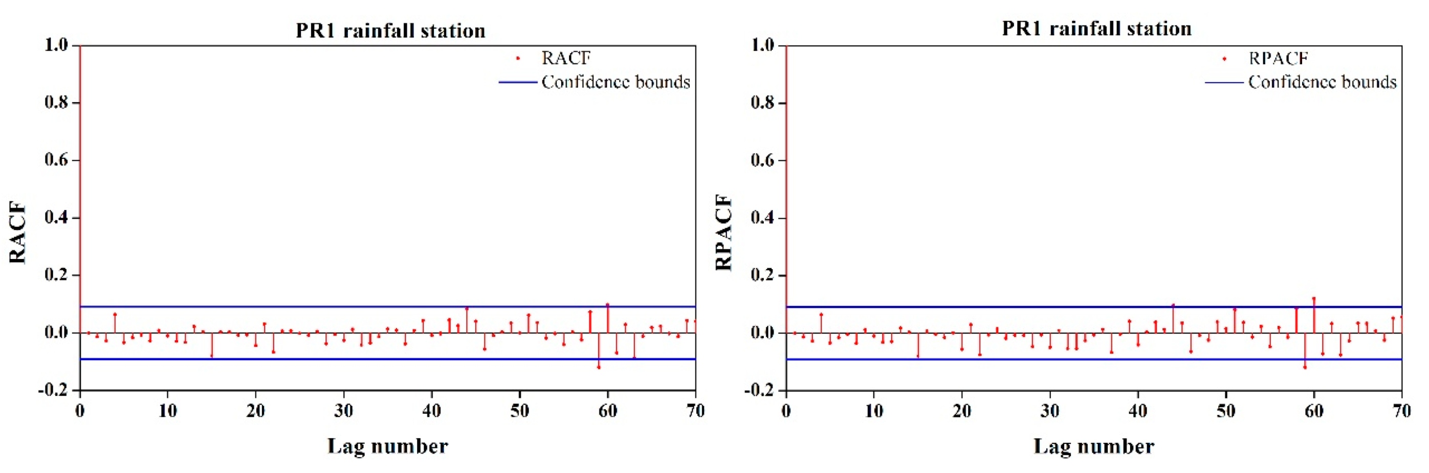
The independence of the residuals was checked by a correlogram and the LBQ test. Figure 3 shows the RACF and RPACF. The results show that most of the RACF and RPACF values were within the confidence limit, which implies that the residuals did not exhibit a significant correlation with each other. For the second method, the LBQ test was employed in this study to determine whether the residuals are dependent, and the results are presented in

Table 4. Ljung–Box–Pierce (LBQ) statistics for the residuals at each basin.

LBQ Test
Station	PR1	BR1	GR1	YR2	RR2	KR3	LR2
Test statistic (Q)	55.33	58.41	73.58	53.91	41.43	37.89	48.18
Critical value	89.39	89.39	89.39	89.39	89.39	89.39	89.39

Degrees of freedom = 69; significance level = 0.05.

. We can observe that the computed statistics were less than the critical values at each station, which also indicates there was no significant correlation between the residuals, and the residuals from the selected model were in accordance with white noise.

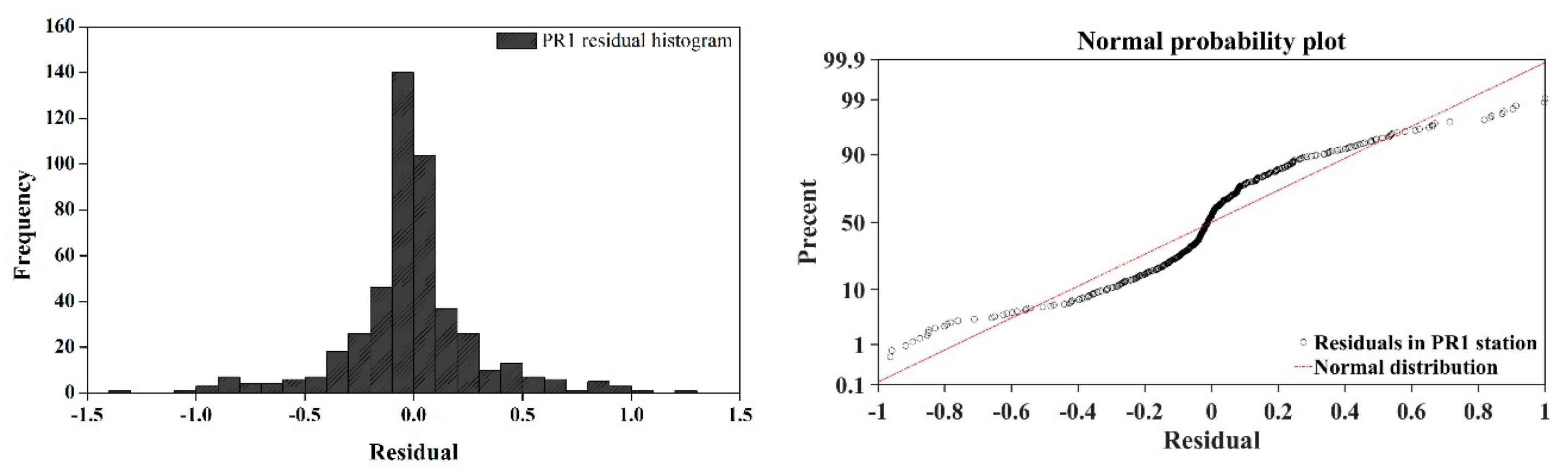
Figure 4 depicts the histogram and normal probability plot of the residuals at the PR1 station in the Pozi River basin. The histograms show that the residuals were roughly centered on zero and were more or less normally distributed [13,33]. The normal probability plot of the residuals indicates that the residuals lay on a diagonal line, which represents the normal probability for residuals in each basin [13,34]. Therefore, both methods provided evidence of the normality of the residuals.

To determine whether the ability of the model to predict variable values is consistent, it is important to verify the homoscedasticity of the residuals [35]. The homoscedasticity of the residuals was checked by the scatterplot of the residuals against predicted values. The results are shown in Figure 5. The plot exhibited no pattern, and the residuals were randomly scattered. That is, the residuals were evenly distributed around a zero mean, which implies that the model was well fitted.

According to the above check, the residuals of the model were uncorrelated, had constant variance, and were normally distributed, and the statistical properties of the residuals were compliant with white noise. Thus, we confirmed that the selected model is adequate for the corresponding SPI time series at each station.

4.4. Model Validation

Here, we utilized data from 2007 to 2017 for model validation. Figure 6 presents a comparison of the observed data with predicted values at each basin using the best SARIMA model. The predicted value yielded a similar pattern to the observed data, and the performance measures are presented in

Table 5. Performance measures for the selected model for the observed data and predicted values.

Station	Model	Performance Measures
		R2	RMSE	MAE
PR1	ARIMA(1,1,0)(3,0,4)12	0.8775	0.3220	0.2159
BR1	ARIMA(1,1,0)(3,0,4)12	0.8869	0.3628	0.2291
GR1	ARIMA(1,1,0)(4,0,4)12	0.8938	0.3241	0.2120
YR2	ARIMA(1,1,0)(2,0,3)12	0.8445	0.3123	0.2060
RR2	ARIMA(1,1,0)(2,0,4)12	0.8602	0.3482	0.2239
KR3	ARIMA(1,1,0)(3,0,3)12	0.8337	0.3699	0.2339
LR2	ARIMA(1,1,0)(3,0,3)12	0.8213	0.3714	0.2281

Abbreviations: RMSE—root-mean-square error, MAE—mean absolute error.

. In general, the higher the R² value, the better the performance of the model. According to our results, the R² values in each station were greater than 0.8, and the root-mean-square error (RMSE) and mean absolute error (MAE) were also sufficiently low. Therefore, the SARIMA model used to predict drought index in this study is reasonably precise.

4.5. Forecasting

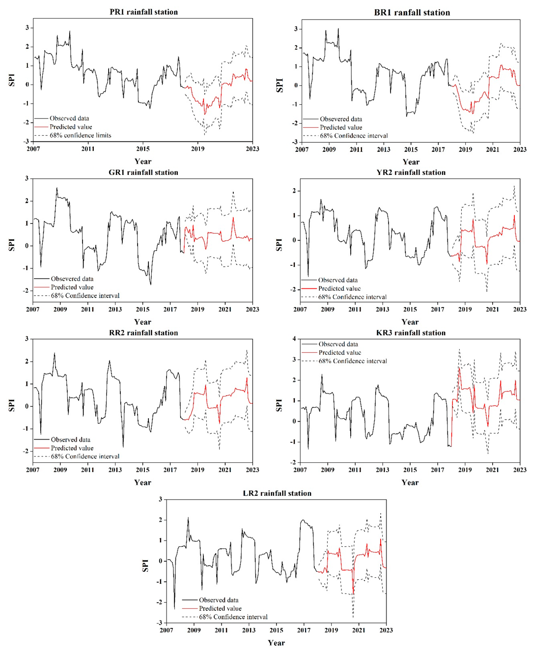
The reason that drought forecasting is necessary for water resource management and planning is that drought events can then be diagnosed in advance, so that experts can take precautions. In this study, we employed the seasonal ARIMA model to forecast the drought condition in the next four years, from 2019 to 2022. The results at each basin are depicted in Figure 7. It was observed that the predicted values showed stochastic change for each SPI time series. According to the analytical results, the lowest SPI values were concentrated in the summer, which means that this region may be affected by drought in the summer in the future. In general, the main source of rainfall in Taiwan during the summer is typhoons. Typhoons can introduce abundant water resources. However, if the number of typhoons is small or the typhoons do not directly affect Taiwan, this sometimes results in a water shortage in the summer. In 2018, the number of typhoons generated between June and September was as high as 22. This is the year in which the most typhoons occurred in the past 10 years. However, only two typhoons affected Taiwan, which may have led to insufficient summer rainfall in Taiwan [36]. In addition, the Pacific high is the main climate factor during the summer in Taiwan, and this is becoming stronger owing to climate change [37], making Taiwan’s climate hotter and with less precipitation. The Pacific high also guides the paths of typhoons. If the western edge of the Pacific high extends westward to the Asian continent, then a typhoon may pass through the Philippines instead of Taiwan. This is one of the reasons why there were fewer typhoons in 2018 in Taiwan. In recent years, the Pacific high has exhibited a tendency to move increasingly westward [38]. Therefore, the summer climate of Taiwan may change in the future under climate change. However, the details remain to be discussed in future research. In this study, the ARIMA model was employed to forecast drought events in the future. Unlike previous studies, we used a stochastic rather than deterministic method to describe the forecasting results. According to historical drought events in Taiwan, drought events occur approximately every three to four years. There was a water shortage situation in 2017 in Taiwan, and 2020 may be a drier year, which is consistent with the results we found in this study. A statistical method involves establishing suitable models to characterize climate factors such as precipitation. Stationarity is generally assumed to exist between predictor and historical data, but this is not always true. Thus, the uncertainty of the model may be higher. In addition, there are many factors that affect environmental changes, and this may present a challenge under this situation. Further studies should consider climate variability in the model for drought forecasting.

5. Conclusions

In this study, the ARIMA model was employed as a drought forecasting tool in southern Taiwan. We used data from 1967 to 2006 to train the model. The model development included three steps: model identification, parameter estimation, and diagnostic checking. In the model identification step, we selected the general form of the model and chose the model with the minimum AIC and SBC as the best fit. In the parameter estimation step, we utilized several statistics to determine whether the parameters we estimated were significant. The results showed that most of the model parameters had p-values below the alpha level (0.05). The diagnostic checking step indicated that the statistical properties of the model residuals were compliant with white noise, including being uncorrelated with a constant variance and normal distribution. Then, the data from 2007 to 2017 were used to validate the model. The results showed that there was a high coefficient of determination (R²) at each station (all over 0.80) and low values for the RMSE and MAE, which implies that the model is adequately precise at each basin. Finally, we used the ARIMA model to forecast the future drought conditions from 2019 to 2022. The forecasting results demonstrate that the SPI value is relatively low in the summer of 2020, which implies that there may be a water shortage in southern Taiwan. This phenomenon may be related to climate change, which leads to an enhancement of the Pacific high extending westward, thus affecting the paths of typhoons. In addition, the Pacific high dominates the summer climate in Taiwan, and if its intensity continues to increase, this will reduce precipitation in Taiwan in the future. However, the detailed evolution mechanism still remains to be discussed in the future.

The stochastic models selected for forecasting the SPI time series provided information on precipitation in southern Taiwan. This is a powerful tool, which can also be used to describe the hydrological time series. The ARIMA model used in this study, based on the SPI, can be applied to forecast drought impacts, playing a vital role in mitigating drought in water resource systems. However, the corresponding natural phenomena are complicated, owing to the influences of many factors. Stochastic models do not consider physical processes, and so it is difficult to understand the physical mechanisms of climate change. In addition, the assumption of the model may lead to higher uncertainty. Nevertheless, the model can be used to predict future trends and serve as a variable for other physical models in further studies.

References

- Dai, A. Increasing drought under global warming in observations and models. Nat. Clim. Chang. 2013, 3, 52–58. [Google Scholar] [CrossRef]
- Habibi, B.; Meddi, M.; Torfs, P.J.; Remaoun, M.; Van Lanen, H.A. Characterisation and prediction of meteorological drought using stochastic models in the semi-arid Chéliff–Zahrez basin (Algeria). J. Hydrol. Reg. Stud. 2018, 16, 15–31. [Google Scholar] [CrossRef]
- Tsakiris, G. Drought Risk Assessment and Management. Water Resour. Manag. 2017, 31, 3083–3095. [Google Scholar] [CrossRef]
- Belayneh, A.; Adamowski, J.; Khalil, B.; Ozga-Zielinski, B. Long-term SPI drought forecasting in the Awash River Basin in Ethiopia using wavelet neural network and wavelet support vector regression models. J. Hydrol. 2014, 508, 418–429. [Google Scholar] [CrossRef]
- Bordi, I.; Sutera, A. Drought monitoring and forecasting at large scale. In Methods and Tools for Drought Analysis and Management 2007; Springer: Dordrecht, The Netherlands, 2017; pp. 3–27. [Google Scholar]
- Mishra, A.K.; Singh, V.P. Drought modeling—A review. J. Hydrol. 2011, 403, 157–175. [Google Scholar] [CrossRef]
- Mossad, A.; Alazba, A.A. Drought forecasting using stochastic models in a hyper-arid climate. Atmosphere 2015, 6, 410–430. [Google Scholar] [CrossRef]
- Panu, U.S.; Sharma, T.C. Challenges in drought research: Some perspectives and future directions. Hydrol. Sci. J. 2002, 47, S19–S30. [Google Scholar] [CrossRef]
- Li, J.; Zhou, S.; Hu, R. Hydrological drought class transition using SPI and SRI time series by loglinear regression. Water Resour. Manag. 2016, 30, 669–684. [Google Scholar] [CrossRef]
- Park, S.; Im, J.; Jang, E.; Rhee, J. Drought assessment and monitoring through blending of multi-sensor indices using machine learning approaches for different climate regions. Agric. For. Meteorol. 2016, 216, 157–169. [Google Scholar] [CrossRef]
- Durdu Ömer, F. Application of linear stochastic models for drought forecasting in the Büyük Menderes river basin, western Turkey. Stoch. Environ. Res. Risk Assess. 2010, 24, 1145–1162. [Google Scholar] [CrossRef]
- Bazrafshan, O.; Salajegheh, A.; Bazrafshan, J.; Mahdavi, M.; Fatehi Maraj, A. Hydrological drought forecasting using ARIMA models (Case study: Karkheh Basin). Ecopersia 2015, 3, 1099–1117. [Google Scholar]
- Mahmud, I.; Bari, S.H.; Rahman, M.T.U. Monthly rainfall forecast of Bangladesh using autoregressive integrated moving average method. Environ. Eng. Res. 2016, 22, 162–168. [Google Scholar] [CrossRef] [Green Version]
- Karthika, K.; Thirunavukkarasu, V.; Karthika, M. Forecasting of meteorological drought using ARIMA model. Indian J. Agric. Res. 2017, 51, 103–111. [Google Scholar] [CrossRef] [Green Version]
- Rahmat, S.N.; Jayasuriya, N.; Bhuiyan, M.A. Short-term droughts forecast using Markov chain model in Victoria, Australia. Theor. Appl. Climatol. 2017, 129, 445–457. [Google Scholar] [CrossRef]
- Agboola, A.H.; Gabriel, A.J.; Aliyu, E.O.; Alese, B.K. Development of a fuzzy logic based rainfall prediction model. Int. J. Eng. Technol. 2013, 3, 427–435. [Google Scholar]
- Jalalkamali, A.; Moradi, M.; Moradi, N. Application of several artificial intelligence models and ARIMAX model for forecasting drought using the Standardized Precipitation Index. Int. J. Environ. Sci. Technol. 2015, 12, 1201–1210. [Google Scholar] [CrossRef]
- Borji, M.; Malekian, A.; Salajegheh, A.; Ghadimi, M. Multi-time-scale analysis of hydrological drought forecasting using support vector regression (SVR) and artificial neural networks (ANN). Arab. J. Geosci. 2016, 9, 725. [Google Scholar] [CrossRef]
- Kousari, M.R.; Hosseini, M.E.; Ahani, H.; Hakimelahi, H. Introducing an operational method to forecast long-term regional drought based on the application of artificial intelligence capabilities. Theor. Appl. Climatol. 2017, 127, 361–380. [Google Scholar] [CrossRef]
- Sheffield, J.; Wood, E.; Chaney, N.; Guan, K.; Sadri, S.; Yuan, X.; Olang, L.; Amani, A.; Ali, A.; DeMuth, S.; et al. A drought monitoring and forecasting system for sub-Sahara African water resources and food security. Bull. Am. Meteorol. Soc. 2014, 95, 861–882. [Google Scholar] [CrossRef]
- Dehghani, M.; Saghafian, B.; Rivaz, F.; Khodadadi, A. Evaluation of dynamic regression and artificial neural networks models for real-time hydrological drought forecasting. Arab. J. Geosci. 2017, 10, 266. [Google Scholar] [CrossRef]
- Alsharif, M.H.; Younes, M.K.; Kim, J. Time series ARIMA model for prediction of daily and monthly average global solar radiation: The case study of Seoul, South Korea. Symmetry 2019, 11, 240. [Google Scholar] [CrossRef]
- Mishra, A.K.; Desai, V.R. Drought forecasting using stochastic models. Stoch. Environ. Res. Risk Assess. 2005, 19, 326–339. [Google Scholar] [CrossRef]
- McKee, T.B.; Doesken, N.J.; Kleist, J. The relationship of drought frequency and duration to time scales. In Proceedings of the Eighth Conference on Applied Climatology, Boston, MA, USA, 17–22 January 1993; Volume 17, pp. 179–183. [Google Scholar]
- WMO. Standardized Precipitation Index User Guide; Svoboda, M., Hayes, M., Wood, D.A., Eds.; WMO: Geneva, Switzerland, 2012. [Google Scholar]
- Bari, S.H.; Rahman, M.T.; Hussain, M.M.; Ray, S. Forecasting monthly precipitation in Sylhet city using ARIMA model. Civ. Environ. Res. 2015, 7, 69–77. [Google Scholar]
- Box, G.E.P.; Jenkins, G.M. Time Series Analysis: Forecasting and Control; Holden-Day: San Francisco, CA, USA, 1976. [Google Scholar]
- Box, G.E.P.; Jenkins, G.M.; Reinsel, G.C. Time Series Analysis, Forecasting and Control; Prentice Hall: Englewood Cliffs, NJ, USA, 1994. [Google Scholar]
- Modarres, R. Streamflow drought time series forecasting. Stoch. Environ. Res. Risk Assess. 2007, 21, 223–233. [Google Scholar] [CrossRef]
- Brockwell, P.J.; Davis, R.A. Introduction to Time Series and Forecasting; Springer Science and Business Media LLC: Berlin/Heidelberg, Germany, 2016. [Google Scholar]
- Akaike, H. A New look at the statistical model identification. Funct. Shape Data Anal. 1974, 19, 215–222. [Google Scholar]
- Schwarz, G. Estimating the dimension of a model. Ann. Stat. 1978, 6, 461–464. [Google Scholar] [CrossRef]
- Rahman, M.A.; Yunsheng, L.; Sultana, N. Analysis and prediction of rainfall trends over Bangladesh using Mann–Kendall, Spearman’s rho tests and ARIMA model. Meteorol. Atmos. Phys. 2017, 129, 409–424. [Google Scholar] [CrossRef]
- Widowati; Putro, S.P.; Koshio, S.; Oktaferdian, V. Implementation of ARIMA model to asses seasonal variability macrobenthic assemblages. Aquat. Procedia 2016, 7, 277–284. [Google Scholar] [CrossRef]
- Huang, Y.F.; Mirzaei, M.; Yap, W.K. Flood analysis in Langat river basin using stochastic model. Int. J. GEOMATE 2016, 11, 2796–2803. [Google Scholar]
- Central Weather Bureau, Monthly Report on Climate System: Typhoon Climate Analysis; Central Weather Bureau, Ministry of Transportation and Communications: Taipei, Taiwan, 2019.
- Li, W.; Li, L.; Ting, M.; Liu, Y. Intensification of Northern Hemisphere subtropical highs in a warming climate. Nat. Geosci. 2012, 5, 830–834. [Google Scholar] [CrossRef]
- Taiwan Climate Change Projection and Information Platform (TCCIP). Taiwan Climate Change Science Report 2017—Physical Phenomena and Mechanisms; TCCIP: Taipei, Taiwan, 2017. [Google Scholar]
Figure 1.
Spatial distribution of the elevation and rainfall stations at each basin.
Figure 2.
Autocorrelation function (ACF) and partial autocorrelation function (PACF) plots for model selection at the PR1 station in the Pozi River basin.
Figure 3.
The ACF and PACF of residuals at the PR1 station in the Pozi River basin.
Figure 4.
The histogram (left column) and normal probability plot (right column) of residuals at the PR1 station in the Pozi River basin.
Figure 5.
The scatterplot of the residuals against predicted values at the PR1 station.
Figure 6.
Comparison of observed data with predicted values using the best seasonal ARIMA (SARIMA) model at each basin.
Figure 7.
Drought forecasting for the period 2018–2022 using the seasonal ARIMA model at each basin.