Improving Parameter Transferability of GR4J Model under Changing Environments Considering Nonstationarity

Abstract

Hydrological nonstationarity has brought great challenges to the reliable application of conceptual hydrological models with time-invariant parameters. To cope with this, approaches have been proposed to consider time-varying model parameters, which can evolve in accordance with climate and watershed conditions. However, the temporal transferability of the time-varying parameter was rarely investigated. This paper aims to investigate the predictive ability and robustness of a hydrological model with time-varying parameter under changing environments. The conceptual hydrological model GR4J (Génie Rural à 4 paramètres Journalier) with only four parameters was chosen and the sensitive parameters were treated as functions of several external covariates that represent the variation of climate and watershed conditions. The investigation was carried out in Weihe Basin and Tuojiang Basin of Western China in the period from 1981 to 2010. Several sub-periods with different climate and watershed conditions were set up to test the temporal parameter transferability of the original GR4J model and the GR4J model with time-varying parameters. The results showed that the performance of streamflow simulation was improved when applying the time-varying parameters. Furthermore, in a series of split-sample tests, the GR4J model with time-varying parameters outperformed the original GR4J model by improving the model robustness. Further studies focus on more diversified model structures and watersheds conditions are necessary to verify the superiority of applying time-varying parameters.

1. Introduction

The conceptual hydrological models are simplified representations of the complex rainfall-runoff processes in the real world. Hence, great emphases are placed on the calibration of parameters to improve the performance of hydrological models. The optimal constant parameter set for a catchment can be inferred using various approaches [1,2] under the assumption that both the climate and the catchment characteristics are stationary. However, the ability to produce reliable predictions with the constant parameter set has been challenged under changing climate and watershed conditions [3,4,5,6,7,8].

The transferability of the model parameters between periods with different climate and watershed conditions is essential for reliable application of the hydrological models. Plenty of previous studies have revealed the fact that model parameters are strongly dependent on the data period with which the hydrological models are calibrated [9,10,11]. In general, loss of robustness and variation in model performance can be witnessed when the model parameters are inappropriately transferred [12]. For example, a model calibrated under wet conditions is usually unlikely to perform well under dry conditions and vice versa. In addition, the optimal parameter set may become no longer suitable once the watershed conditions change significantly as a result of human activities (e.g., the construction of dams, afforestation and deforestation). The impact of such changes on hydrologic processes such as streamflow has been well documented [13,14]. In such cases, hydrological models with time-invariant parameters may show a poor predictive performance due to their inability to explicitly represent the changes within the catchment.

One approach to make the model perform robustly under changing environments is to identify the optimal parameter set with time consistent performance [15,16,17,18,19,20,21,22]. Such approach is based on a series of calibration procedures on different sub-periods, and careful identification of the parameter sets with consistent performance for all these sub-periods. All parameter sets are independently evaluated in every sub-period, and only the parameter set that performs well in all cases are finally selected. Nevertheless, this is achieved at the cost of a possible decline in model performance for some individual sub-periods.

Another approach to improve the predictive performance of hydrological models under changing environments is to allow model parameters to evolve over time [23,24,25,26,27,28,29,30,31,32,33]. For example, Wallner and Haberlandt [25] linked the time-varying model parameters of a modified version of the HBV (Hydrologiska Byråns Vattenbalansavdelning) model with the climate indices. The results showed a significant improvement in model performance for streamflow simulation when using the time-varying parameters, especially for low flows. Pathiraja et al. [26] demonstrated the potential for the data assimilation method to detect the temporal variation in all parameters of the Probability Distributed Model and to improve model performance for streamflow simulation. Westra et al. [27] reported a significantly improved streamflow simulation performance of the GR4J model when the parameter represents the production storage capacity was made dependent on covariates describing seasonality, annual variability, and longer-term trends. Deng et al. [28] assumed the parameters of the two-parameter monthly water balance model to be time-varying as functions of catchment properties. Their case study in southern China suggests that the incorporation of time-varying parameters can enhance the capability of hydrological models to produce reliable predictions under changing environments. These studies suggest that the time-varying parameter may serve as an effective compensation for the possible deficiency of model structure, which failed to represent changes in hydrological dynamics within the watershed.

However, few recent studies focus on the temporal transferability of the time-varying parameters (i.e., robustness under extrapolation). Some previous studies [25,27,28] have tested the temporal transferability of the time-varying parameter from only one calibration period to only one validation period. They reported that the streamflow simulation using a model with the time-varying parameter is better than the original model during the validation procedure. However, these studies failed to fully account for the cases where time-varying parameter is transferred between periods with contrasting climate and watershed conditions (e.g., from driest period to wettest period), which remains an interesting topic that deserves further researches.

This study aims to investigate whether a hydrological model with time-varying parameter would achieve a better streamflow simulation performance and parameter transferability under changing environments than its original form. The GR4J model was chosen for its simplicity in model structure and parsimony in model parameters [34]. The relatively sensitive parameters of the GR4J model were treated as time-varying and assumed to be a function of several external covariates. Several sub-periods with different climate and watershed conditions were set up for a series of split-sample test for the GR4J model with constant parameter and time-varying parameter. The investigation was carried out for Weihe Basin and Tuojiang Basin in western China.

2. Methodology

2.1. The Original GR4J Model and GR4J Model with Time-Varying Parameter

The original GR4J model has four parameters, namely the production storage capacity $x_1$, the groundwater exchange coefficient $x_2$, the one day ahead maximum capacity of the routing storage $x_3$ and the time base of unit hydrograph $x_4$, as presented in

Table 1. Description of the GR4J model parameters.

Parameter	Description	Unit	Feasible Range
			Lower Bound	Upper Bound
$x_1$	production storage capacity	mm	20	1200
$x_2$	groundwater exchange coefficient	mm	−5	3
$x_3$	one day ahead maximum capacity of the routing store	mm	20	500
$x_4$	time base of unit hydrograph	days	1	5

. More details about the GR4J model can be found in the work of Perrin et al. [34].

A comprehensive sensitivity analysis of all four parameters is needed to determinate which parameter is relatively more sensitive and should be treated as time-varying. To this end, the Sobol’ sensitivity analysis method [35] was applied in this study. Considering that this study focuses on changing environments where stationary rainfall-runoff relationship is usually absent, the Sobol’ sensitivity indices were computed at the monthly timescale. This temporally discretized sensitivity analysis was expected to provide significant information about model behavior and capture the diversity of parameter sensitivity during different periods [36].

The GR4J model with time-varying parameters is referred to as GR4J-T model hereafter. The selected time-varying parameters are treated as functions of several external covariates related to the alternation of climate or watershed conditions. The potential covariates for time-varying parameters are denoted as $V_j(j=1,2,\dots ,M)$ and their long-term mean values as ${\overline{V}}_j(j=1,2,\dots ,M)$, where $M$ is the total number of the external covariates. When the parameter $x_i(i=1,2,3,4)$ of the GR4J model is considered to be time-varying, it is denoted as $x_{i,t}$, where t indicates the time. The general relationship of $x_{i,t}$ with the corresponding external covariates is assumed to be,

$$\frac{x_{i,t}-x_{i,c}}{x_{i,c}}={\displaystyle \sum _{j=1}^M{\beta }_{i,j}{f}_j\left(\frac{V_{j,t}-\overline{V_j}}{\overline{V_j}}\right)}$$

(1)

which can be rewritten as,

$$x_{i,t}=x_{i,c}+{\displaystyle \sum _{j=1}^M{\lambda }_{i,j}{f}_j\left(\frac{V_{j,t}}{\overline{V_j}}-1\right)}$$

(2)

where $x_{i,c}$ stands for the constant value of parameter $x_i$ over the calibration period, while ${\beta }_{i,j}$ and ${\lambda }_{i,j}$ $({\lambda }_{i,j}={\beta }_{i,j}\cdot x_{i,c})$, $j=1,\dots ,M$, are the corresponding regression parameters. The $f_j(\cdot )$ is the link function between the time-varying parameter $x_{i,t}$ and the external covariate $V_j$, which can take multiple forms such as $f(z)=z$ (linear), $f(z)=e^z$ (exponential), or $f(z)=\ln (z+1)$ (logarithmic), so as to account for possible linear or non-linear relationship of the time-varying parameter with the external covariates.

Choosing suitable external covariates is a critical issue for the utilization of Equation (1) and (2), but it is usually limited by the availability of dataset. Considering that in practice the daily changes in any external covariates could only cause negligible changes in the time-varying parameters, so only impacts of the monthly changes in any physical covariates on the parameter were investigated in this study, i.e., the time-varying parameters were updated monthly in every simulation run. Inspired by recent work [27,28], 8 external covariates related to variation of climate or watershed underlying conditions, including 1-month, 2-month and 3-month antecedent monthly precipitation and potential evapotranspiration (P₁, P₂, P_3, PET₁, PET₂ and PET₃) and NDVI (Normalized Difference Vegetation Index) of current month (NDVI₀), one-month shifted NDVI (NDVI₁) (as shown in

Table 2. Description of external covariates for time-varying parameters.

Covariates	Unit	Description
P1	mm	One-month antecedent monthly total precipitation
P2	mm	Two-month antecedent monthly total precipitation
P3	mm	Three-month antecedent monthly total precipitation
PET1	mm	One-month antecedent monthly total potential evapotranspiration
PET2	mm	Two-month antecedent monthly total potential evapotranspiration
PET3	mm	Three-month antecedent monthly total potential evapotranspiration
NDVI0	-	NDVI value for the current month
NDVI1	-	NDVI value for the previous month

), were considered as candidate covariates for the time-varying parameter.

2.2. Model Calibration and Evaluation

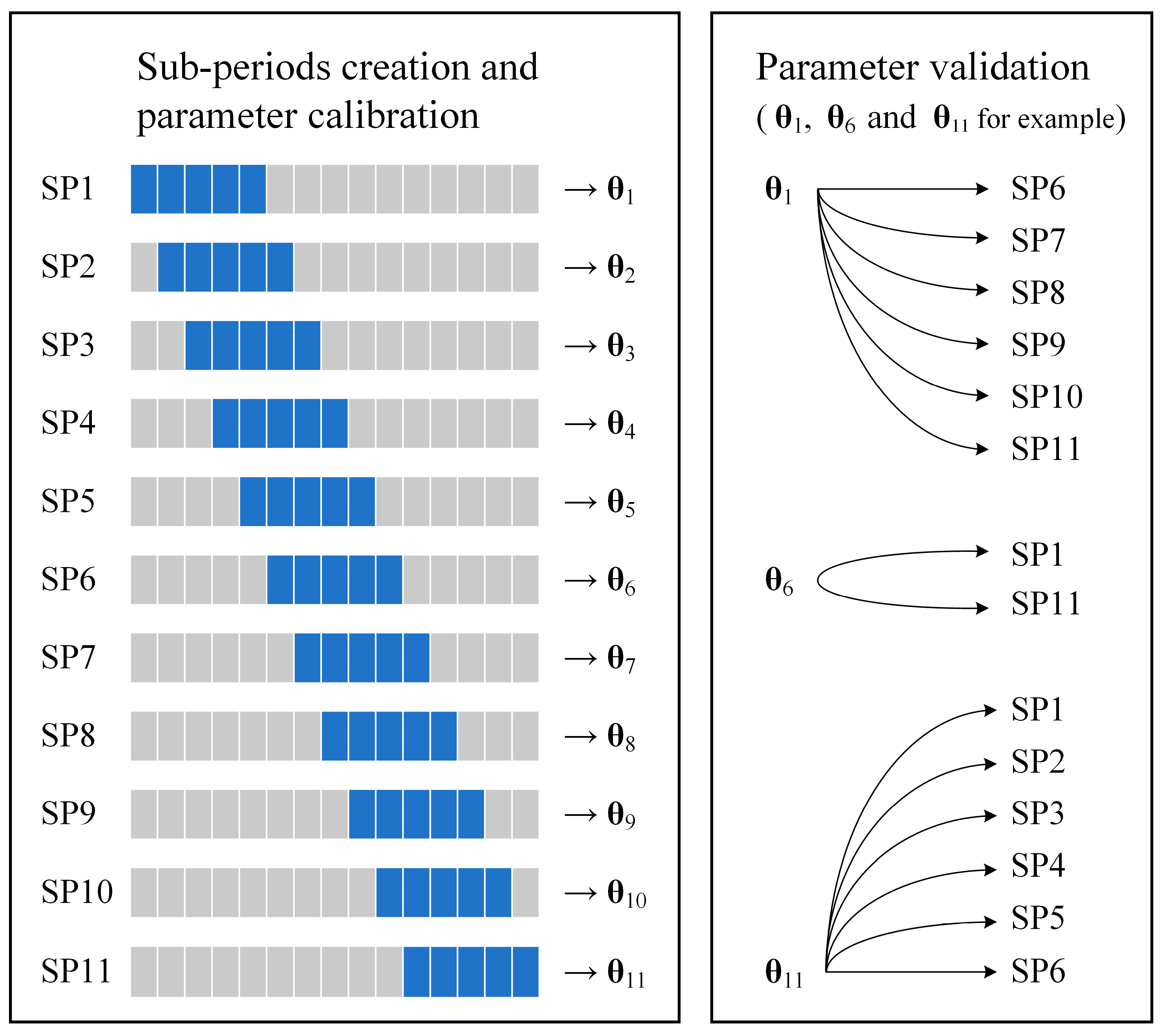
The differential split-sample test (DSST) is a common way to evaluate hydrological models between sub-periods with contrasting climate and watershed underlying conditions [37,38]. In practice, usually only two or three contrasting sub-periods can be identified due to the availability of the hydro-meteorological data. This may limit the potential of DSST for accessing the transferability of model parameters and drawing general conclusions. To overcome this limitation, the generalized split-sample test (GSST) proposed by Coron et al. [39,40] was chosen to test the temporal transferability of parameter for the GR4J and GR4J-T model in this study. The main objective of GSST procedure is to evaluate the model performance under as many and as varied climatic and watershed conditions as possible. To this end, a sliding window with a specific length (e.g., five years) is applied to define the sub-periods (as illustrated in Figure 1). In Figure 1, the blue bars indicate the sub-periods while the grey bars represent the remaining part of the time series. Between two adjacent sub-periods, the sliding window is moved by one year.

When the sub-periods creation completed, both the GR4J and GR4J-T model were calibrated in each sub-period. Then the parameter sets obtained was used to perform validation test on independent sub-periods, i.e., the sub-periods that do not overlap with the calibration sub-period. For example, the parameter calibrated during SP1 won’t be validated in SP2, SP3, SP4 and SP5, as illustrated in Figure 1. For more detail about GSST, the readers can refer to the work of Coron et al. [39,40].

The original GR4J model and the GR4J-T model have different numbers of calibrated parameters. For the original GR4J model, the number of calibrated parameters is 4, i.e., $\mathsf{\theta }=\{x_1,x_2,x_3,x_4\}$. In the case of the GR4J-T model, when the parameter $x_i(i=1,2,3,4)$ is treated to be time-varying, its constant value $x_{i,c}$ and the corresponding regression parameters ${\lambda }_{i,j}(j=1,\dots ,M)$ are calibrated together with other time-invariant parameters. For example, when only the parameter $x_1$ is regarded as the time-varying parameter, parameters that require calibration are $\mathsf{\theta }=\{x_{1,c},{\lambda }_{1,1},\dots ,{\lambda }_{1,M},x_2,x_3,x_4\}$. Similarly, when multiple parameters are assumed to be time-varying, e.g., $x_1$ and $x_2$, the calibrated parameters become $\mathsf{\theta }=\{x_{1,c},{\lambda }_{1,1},\dots ,{\lambda }_{1,M},x_{2,c},{\lambda }_{2,1},\dots ,{\lambda }_{2,M},x_3,x_4\}$.

The widely used Kling-Gupta Efficiency (KGE) [41] was applied to assess the overall performance of the GR4J and GR4J-T model. The KGE is calculated as follows,

$$KGE=1-\sqrt{{\left(r(Q_{act},Q_{sim})-1\right)}^2+{\left(\frac{\mu (Q_{act})}{\mu (Q_{sim})}-1\right)}^2+{\left(\frac{\sigma (Q_{act})}{\sigma (Q_{sim})}-1\right)}^2}$$

(3)

where $Q_{act}$ and $Q_{sim}$ are the observed and model-simulated streamflow series, respectively, $r(Q_{act},Q_{sim})$ is the Pearson’s correlation coefficient between the observed and simulated streamflow series, $\mu (Q_{act})$ and $\mu (Q_{sim})$ are the mean values of the observed and simulated streamflow series, respectively, $\sigma (Q_{act})$ and $\sigma (Q_{sim})$ are the standard deviation of the observed and simulated streamflow series, respectively. KGE value ranges from $-\infty$ to 1, with a value closer to 1 indicating a better simulation performance.

The bias between the observed and simulated streamflow (BIAS) was also applied, which is calculated as follows,

$$BIAS=\frac{{\displaystyle {\sum }_{t=1}^T{Q}_{sim}(t)}}{{\displaystyle {\sum }_{t=1}^T{Q}_{act}(t)}}-1$$

(4)

where $Q_{act}(t)$ and $Q_{sim}(t)$ are the observed and model-simulated streamflow at time $t$, respectively. BIAS with a value of 0 indicates no bias, and a value above 0 means an overestimation of the total streamflow volume.

Both the GR4J and GR4J-T models were calibrated using the SCEM (Shuffled Complex Evolution Metropolis) optimization algorithm [2,42], which has been widely used for practical assessment of parameter uncertainty in hydrological modeling. The SCEM algorithm, partially inspired by the SCE-UA (Shuffled Complex Evolution - University of Arizona) algorithm [1], merges the strengths of Metropolis-Hastings sampling [43,44], controlled random search, competitive evolution and complex shuffling to evolve a population of sampled points to an approximation of the posterior distribution of the parameters. Besides, the SCEM method can identify the most likely parameter set and meanwhile its underlying posterior probability distribution in every single run [45]. The likelihood of a parameter set was calculated as the corresponding KGE value. Considering that the likelihood value must be nonnegative and monotonically increasing with improved performance, the parameter set that leads to a KGE value below 0 was rejected during the evolution procedure within SCEM. The convergence of the algorithm was determined using the Gelman-Rubin statistic [46], which is calculated on the posterior densities to check whether convergence to a stationary target distribution has been reached. For more detail about the SCEM optimization algorithm, the reader can refer to the work of Vrugt et al. [2].

After the convergence of the SCEM optimization algorithm, the final posterior distribution of parameter can be obtained. In total 5000 parameter sets were sampled from the posterior distribution to account for parameter uncertainty in this study. It should be noted that the 5000 parameter sets can lead to very similar streamflow simulation performance in terms of the KGE criteria, and the one corresponding to the highest KGE value (i.e., the KGE-best) was chosen to represent the estimate of the global optimum and used for the model evaluation and selection.

2.3. Temporal Transferability Test of Model Parameters

When a parameter set $\mathsf{\theta }$ that calibrated from the sub-period D (denoted as “donor period” hereafter) is transferred to the sub-period R (i.e., validation, denoted as “receiver period”), the Kling-Gupta Efficiency (KGE) can be rewritten as,

$$KG{E}_{D\to R}=1-\sqrt{{\left(r(Q_{act,R},Q_{sim,R}[{\mathsf{\theta }}_D])-1\right)}^2+{\left(\frac{\mu (Q_{act,R})}{\mu (Q_{sim,R}[{\mathsf{\theta }}_D])}-1\right)}^2+{\left(\frac{\sigma (Q_{act,R})}{\sigma (Q_{sim,R}[{\mathsf{\theta }}_D])}-1\right)}^2}$$

(5)

where $Q_{act,R}$ is the simulated streamflow series of sub-period R, $Q_{sim,R}[{\mathsf{\theta }}_D]$ is the simulated streamflow series of sub-period R using parameter set obtained from sub-period D. In addition, $KG{E}_{R\to R}$ is defined to access the streamflow simulation performance during sub-period R using parameter sets obtained from sub-period R.

Note that the temporal transferability test on one single parameter set could be less persuasive. To fully evaluate the temporal parameter transferability of both the GR4J and GR4J-T model, the 5000 parameter sets from each sub-period were then validated at other independent sub-periods, and the average performance of both models were compared. To this end, a parameter transferability criteria (PTC) is defined as:

$$PTC=\frac{{\sum }_{n=1}^N{KGE}_{D\to \mathrm{R}}^t(n)-{\sum }_{n=1}^N{KGE}_{D\to \mathrm{R}}^c(n)}{N}$$

(6)

where ${KGE}_{D\to \mathrm{R}}^c(n)$ and ${KGE}_{D\to \mathrm{R}}^t(n)$ represent the ${KGE}_{D\to \mathrm{R}}^{}$ value in the case of the GR4J and the GR4J-T model using the n^th parameter set, respectively. Here, N takes the value of 5000. Note that PTC with a value above 0 indicates a better parameter transferability for the GR4J-T model over the original GR4J model when transferred from sub-period D to sub-period R.

3. Study Data and Area

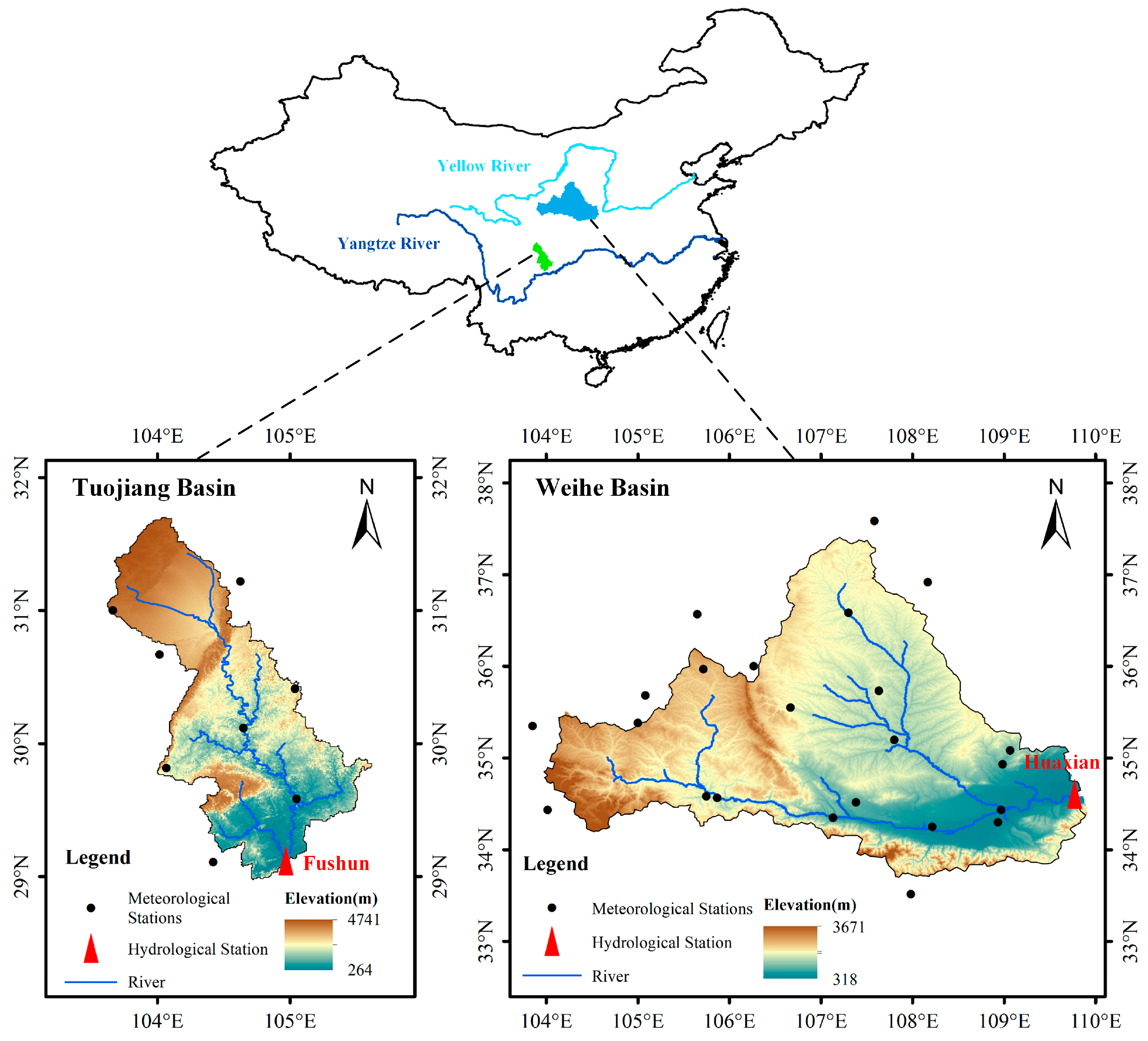
Weihe Basin and Tuojiang Basin in Western China were chosen as the study areas. Weihe Basin is located between the coordinates 33°40′–37°26′ N and 103°57′–110°27′ E, with a drainage area of 148,000 km² above Huaxian hydrological station, as shown in Figure 2. The elevation within Weihe Basin ranges from 3671 m in the western upstream region to 318 m in the eastern downstream region. Dominated by the semi-arid continental monsoon climate, most precipitation and flood events in Weihe Basin occur in late summer and early autumn. For Weihe Basin, climate variability is significant and human activities have been proved to be the main cause of the alternation of flow regimes. Previous studies have shown that the annual streamflow of the gauge Huaxian has been declining over the past decades [47,48,49], mainly due to the increasing human activities including the agricultural irrigation, the construction of large water control projects and the implementation of the water-soil conservation projects [50,51]. In addition, the variations of the annual precipitation have also contributed to the reduced annual streamflow in Weihe Basin [52].

Tuojiang Basin (28°88′–30°29′ N, 105°44′–108°20′ E) is an upstream tributary of the Yangtze River, with a total length of 712 km. Tuojiang Basin covers 19,613 km² with Fushun hydrological station as the catchment outlet. The elevation within Tuojiang Basin ranges from 264 to 4741 m and decreases from northwest to southeast. Tuojiang Basin is dominated by the subtropical monsoon climate, with most precipitation and flood events occurring in summer and early autumn. The annual streamflow of Tuojiang Basin was also in a downtrend. However, few recent studies focus on Tuojiang Basin and the reason for the declined annual streamflow remains unclear.

The input data for the GR4J model include precipitation (P) and potential evapotranspiration (PET). The precipitation and air temperature data were provided by National Meteorological Information Center of China [53] on a daily basis for the period from 1981 to 2010 and has been widely validated for its quality in previous studies [47,48,49]. Limited by availability of the meteorological dataset, the potential evapotranspiration (PET) was calculated using the Blaney-Criddle method [54] from the daily average air temperature and the daily sunshine duration. To calibrate and validate the GR4J model, the observed streamflow (Q) series from the gauge Huaxian and Fushun were obtained for the period 1981–2010. The NDVI dataset for the period from 1981–2010 was obtained from the GIMMS (Global Inventory Modelling and Mapping Studies) NDVI–3g product [55], which has been widely validated [55,56]. Since its temporal resolution is 15-day, the monthly NDVI is represented by the mean value of the two NDVI values in each month.

4. Results and Discussion

4.1. Diagnostics of Hydrological Nonstationarity

Considering the available hydro-meteorological dataset for Weihe Basin and Tuojiang Basin are for the period 1981–2010, in total 26 sub-periods of 5-year in length are set up following the method described in Figure 1. The reasons for the selection of 5-year as the sub-period length are: (1) 5-year is sufficient for continuous hydrological simulation, (2) a large number of sub-periods (26 in this study) can be set up given that only 30-year records were available. To identify the long-term variation of the hydro-meteorological data series of both basins, the non-parametric Mann-Kendall method [57,58] was applied to examine the trends in the annual P, PET, Q and annual runoff ratios (RR) series of the period 1981–2010, and the result is shown in

Table 3. Mann-Kendal (MK) test results of the annual hydro-meteorological data series, the annual runoff ratios and the annual NDVI data series for Weihe Basin and Tuojiang Basin. The critical value of the MK statistic is $Z_{1-\alpha /2}=1.960$ with $\alpha =0.05$.

Basin	Data	Z statistic	Trend
Weihe Basin	Annual P	−1.22	↓
	Annual PET	1.56	↑
	Annual Q	−2.61	↓**
	Annual RR	−2.56	↓**
	Annual NDVI	3.96	↑**
Tuojiang Basin	Annual P	−1.32	↓
	Annual PET	−3.51	↓**
	Annual Q	−2.75	↓**
	Annual RR	−2.78	↓**
	Annual NDVI	0.46	↑

Notes: The symbol “**” indicates a significant uptrend or downtrend.

. The results show a significant downtrend for the annual Q and RR series, a slight downtrend for annual P series and uptrend for the PET series in Weihe Basin. In the case of Tuojiang Basin, a slight downtrend for annual P series and significant downtrend for annual PET, Q, and RR series are presented. It can be found that both basins witnessed a clear nonstationary in rainfall-runoff relationship. In terms of the annual NDVI series, Weihe Basin shows a clear uptrend while Tuojiang Basin shows no clear changes. This may be attributed to the fact that Weihe Basin has experienced an incessant construction of water-soil conservation projects (e.g., afforestation) since the early 1980s [49].

Variability is also apparent between longer periods, as shown in Figure 3, where the relative mean P, PET, Q, and RR values for all sub-periods (5-year sliding window) are plotted for both basins. Figure 3a–d show how the 5-year hydro-meteorological conditions differ from those of the whole period (1981–2010). For each basin, a line corresponds to the series of the mean values over a 5-year sliding window (sub-period). Each value is expressed relative to the mean value of the whole period (1981–2010) and plotted in the middle year of the corresponding sub-period. The result is in line with the results of the MK-test. For both Weihe Basin and Tuojiang Basin, a significant downtrend of 5-year total streamflow volume and a decreased runoff-ratios are presented. This may question the parameter transferability of the GR4J model, which is detailed in following sections.

4.2. Parameter Estimation for the GR4J and GR4J-T Model

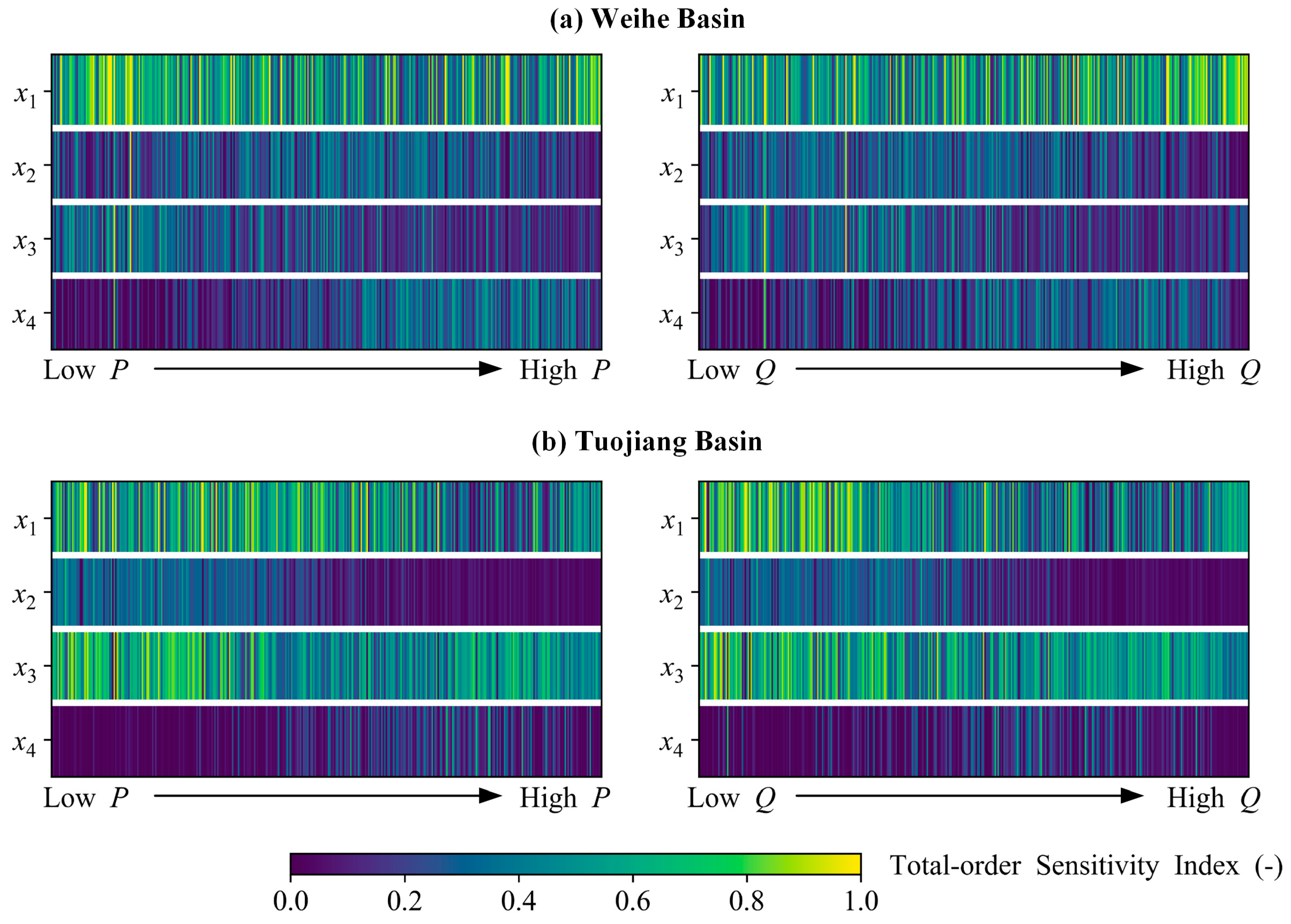
To incorporate time-varying sensitivity analysis, the Sobol’ sensitivity analysis was repeated at a monthly temporal resolution rather than over the whole period (1981–2010). The monthly sensitivity indices (including the first-order and total-order) of each parameter were therefore obtained with KGE as the metric. More detail about the time-varying sensitivity analysis can be found in the work of Herman et al. [36]. Figure 4 provides a simple and direct interpretation of the relationships between the sensitivity of the GR4J’s parameters and changing precipitation and streamflow conditions, which was achieved by sorting the monthly sensitivity indices (only the total-order were presented for brevity) for both basins along ascending gradients of monthly precipitation and streamflow.

For Weihe Basin, the parameter $x_1$, which controls the production storage capacity, shows a strong sensitivity during both high-flow and low-flow months. In contrast, the parameter $x_2$, $x_3$ and $x_4$ are less sensitive. In the case of Tuojiang Basin, the parameter $x_1$ and $x_3$ dominate the months with low-flow and less-precipitation, while the parameter $x_2$ and $x_4$ show relatively weaker sensitivity. Thus, the parameter $x_1$ is assumed to be time-varying for Weihe Basin, and the parameter $x_1$ and $x_3$ for Tuojiang Basin.

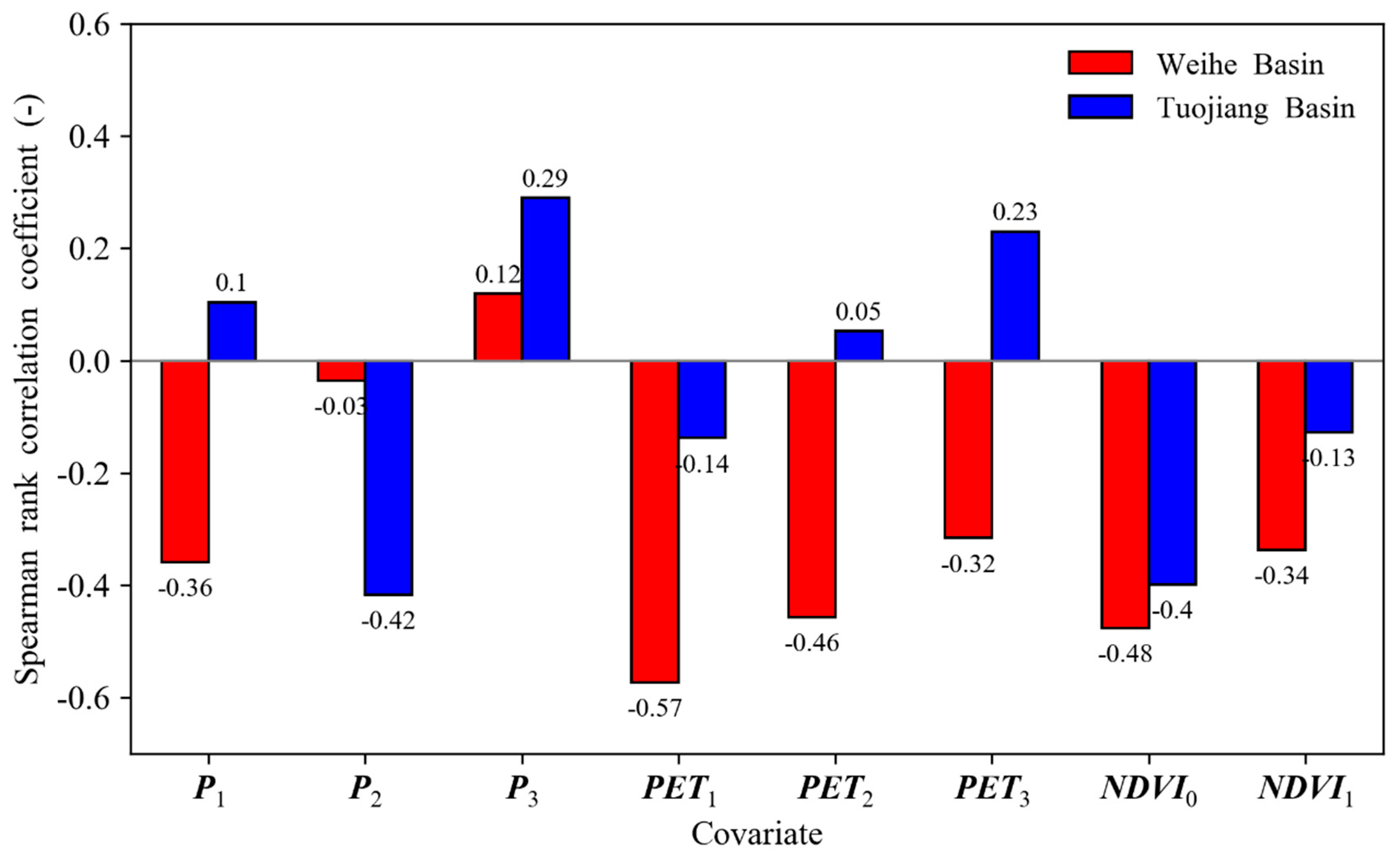
The correlation between monthly runoff-ratios and monthly external covariate is summarized in Figure 5 in term of Spearman’s rank correlation coefficient. Note that the monthly runoff-ratios were calculated as the ratios of monthly runoff depth (mm) and the monthly total precipitation (mm). It can be found that the monthly runoff-ratios has a strong correlation with PET₁ and NDVI₀ for Weihe Basin. In the case of Tuojiang Basin, the covariates with high correlation coefficient are P₂ and NDVI₀. This correlation analysis was done to justify the reasonability of incorporating the abovementioned external covariates into the time-varying parameters. It may be arbitrary to assert that an external covariate with a weak correlation coefficient is inappropriate and useless. In this study, all 8 external covariates were applied to construct the time-varying parameters for both Weihe Basin and Tuojiang Basin, which is detailed in the following section.

To reduce the influence of the initial state, a spin-up period of 1-year was used at the parameter calibration procedure for each sub-period, and the simulated streamflow within the spin-up period was excluded in the model assessment procedure. To fully explore the potential for the GR4J-T model in streamflow simulation, all combination of the eight external covariates were investigated and their corresponding performances were compared in terms of the KGE and BIAS criteria. Considering a large number of model assessment procedure (e.g., 255 covariate combinations for each sub-period in Weihe Basin,$C_8^1+C_8^2+C_8^3+C_8^4+C_8^5+C_8^6+C_8^7+C_8^8=255$), only a small part of the results is presented hereafter for the sake of brevity. For each covariate combination, totally 5000 parameter sets were obtained from the calibration procedure and only the KGE-best for each covariate combination is shown here. For example,

Table 4. Comparison of streamflow simulation performance of the GR4J model (C0) and the GR4J-T model (C1–C7) in Weihe Basin during the sub-period 1 (SP1, from 1981 to 1985).

Case	Covariate			$\mathbf{Equation}\mathbf{for}\mathbf{Time}-\mathbf{Varying}\mathbf{Parameter}{\mathit{x}}_{1,\mathit{t}}$	KGE (-)	BIAS (%)
	${\mathit{P}}_1$	$\mathit{P}\mathit{E}{\mathit{T}}_1$	$\mathit{N}\mathit{D}\mathit{V}{\mathit{I}}_0$
C0				$x_{1,t}=320.1$	0.727	−16.1
C1	✓			$x_{1,t}=290.3+0.28P_{1,t}$	0.752	−6.3
C2		✓		$x_{1,t}=306.5+0.54PE{T}_{1,t}$	0.749	−8.1
C3			✓	$x_{1,t}=296.8+99.8NDV{I}_{0,t}$	0.751	−11.2
C4	✓	✓		$x_{1,t}=271.8+0.19P_{1,t}+0.27PE{T}_{1,t}$	0.755	−6.2
C5	✓		✓	$x_{1,t}=312.5+0.17PE{T}_{1,t}+60.6NDV{I}_{1,t}$	0.759	−6.4
C6		✓	✓	$x_{1,t}=298.4+0.25P_{1,t}+41.8NDV{I}_{0,t}$	0.751	−9.3
C7	✓	✓	✓	$x_{1,t}=303.4+0.18P_{1,t}+0.28PE{T}_{1,t}+32.6NDV{I}_{0,t}$	0.761	−6.1

presented the streamflow simulation performance for 8 different cases (C0–C7) during the sub-period 1 (SP1) in Weihe Basin. The case C0 was designed to represent the original GR4J model, where the value of parameter $x_1$ is invariant over time. Under cases C1–C7, the external covariate $P_1$, $PE{T}_1$ and $NDV{I}_0$ were incorporated into the time-varying parameter $x_{1,t}$. The corresponding equations for time-varying parameter $x_{1,t}$ are also presented in Table 4. It should be noted that three forms of link functions including ‘linear’, ‘exponential’ and ‘logarithmic’ were used to link the external covariates with the time-varying parameter. Three link functions lead to similar model performance, while the ‘linear’ was always the best and simplest one. So only the ‘linear’ is shown here.

It can be found that the streamflow simulation performance significantly improves when parameter $x_1$ was allowed to change over time. For example, the KGE value is 0.752 when only the covariate $P_1$ was considered when compared to 0.727 for the original GR4J model. The difference in BIAS criteria (from −16.1% to −6.3%) also indicates a better water balance simulation of the GR4J model with time-varying parameter. Furthermore, the highest KGE value (0.761) was achieved when $P_1$, $PE{T}_1$ and $NDV{I}_0$ were incorporated into the time-varying parameter.

4.3. Streamflow Simulation Performance of the GR4J and GR4J-T Model

Similarly, the model assessment procedure was repeated for the rest sub-periods (SP2-SP26).

Table 5. Comparison of streamflow simulation performance of the GR4J model and the GR4J-T model in Weihe Basin for all sub-periods (SP1–SP26).

Sub-Period	GR4J Model			GR4J-T Model
	$\mathbf{Value}\mathbf{of}{\mathit{x}}_1$	KGE (-)	BIAS (%)	$\mathbf{Equation}\mathbf{for}\mathbf{Time}-\mathbf{Varying}\mathbf{Parameter}{\mathit{x}}_{1,\mathit{t}}$	KGE (-)	BIAS (%)
SP1	320.1	0.727	−16.1	$x_{1,t}=303.4+0.18P_{1,t}+0.28PE{T}_{1,t}+32.6NDV{I}_{0,t}$	0.761	−6.1
SP2	443.2	0.617	−17.3	$x_{1,t}=278.6+0.16P_{1,t}+0.17PE{T}_{1,t}+57.7NDV{I}_{0,t}$	0.631	−14.5
SP3	324.1	0.571	−19.1	$x_{1,t}=309.2+0.25P_{1,t}-0.14PE{T}_{1,t}-28.6NDV{I}_{0,t}$	0.572	−11.6
SP4	263.5	0.509	−26.2	$x_{1,t}=251.5+0.35P_{1,t}-0.19PE{T}_{1,t}+38.6NDV{I}_{0,t}$	0.591	−20.2
SP5	447.3	0.611	−16.2	$x_{1,t}=399.5+0.27P_{1,t}-0.15PE{T}_{1,t}-4.3NDV{I}_{0,t}$	0.635	−13.2
SP6	375.5	0.389	−22.2	$x_{1,t}=259.1+0.38P_{1,t}-0.21PE{T}_{1,t}+44.6NDV{I}_{0,t}$	0.481	−20.3
SP7	367.4	0.392	−22.9	$x_{1,t}=292.7+0.29P_{1,t}-0.19PE{T}_{1,t}+44.2NDV{I}_{0,t}$	0.514	−27.9
SP8	300.9	0.442	−25.7	$x_{1,t}=251.5+0.35P_{1,t}+0.15PE{T}_{1,t}+21.7NDV{I}_{0,t}$	0.575	−26.4
SP9	256.3	0.341	−23.3	$x_{1,t}=205.6+0.45P_{1,t}-0.37PE{T}_{1,t}+61.9NDV{I}_{0,t}$	0.504	−19.6
SP10	414.5	0.403	−18.1	$x_{1,t}=283.5+0.48P_{1,t}-0.12PE{T}_{1,t}+17.1NDV{I}_{0,t}$	0.442	−15.2
SP11	417.6	0.392	−26.4	$x_{1,t}=233.5+0.17P_{1,t}-0.09PE{T}_{1,t}-7.6NDV{I}_{0,t}$	0.438	−26.6
SP12	244.1	0.483	−25.2	$x_{1,t}=241.5+0.37P_{1,t}-0.49PE{T}_{1,t}+48.2NDV{I}_{0,t}$	0.536	−19.7
SP13	182.4	0.230	−42.9	$x_{1,t}=194.1+0.67P_{1,t}+0.34PE{T}_{1,t}-27.9NDV{I}_{0,t}$	0.432	−40.3
SP14	340.4	0.499	−23.6	$x_{1,t}=305.8+0.47P_{1,t}-0.15PE{T}_{1,t}-34.8NDV{I}_{0,t}$	0.535	−17.9
SP15	424.1	0.659	−13.7	$x_{1,t}=341.5+0.53P_{1,t}-0.09PE{T}_{1,t}-13.6NDV{I}_{0,t}$	0.713	−7.8
SP16	208.1	0.601	−28.2	$x_{1,t}=221.6+0.19P_{1,t}+0.09PE{T}_{1,t}-6.3NDV{I}_{0,t}$	0.622	−26.4
SP17	295.5	0.582	−18.4	$x_{1,t}=329.4+0.54P_{1,t}-0.03PE{T}_{1,t}-28.1NDV{I}_{0,t}$	0.639	−10.1
SP18	315.3	0.489	−24.5	$x_{1,t}=300.7+0.52P_{1,t}-0.35PE{T}_{1,t}-12.2NDV{I}_{0,t}$	0.543	−17.5
SP19	378.7	0.734	−23.3	$x_{1,t}=308.3-0.13P_{1,t}+0.52PE{T}_{1,t}-23.6NDV{I}_{0,t}$	0.763	−16
SP20	429.1	0.779	−21.5	$x_{1,t}=229.8+0.57PE{T}_{1,t}-29.2NDV{I}_{0,t}$	0.801	−17.4
SP21	339.5	0.732	−4.6	$x_{1,t}=325.1-0.51P_{1,t}+0.27PE{T}_{1,t}+29.1NDV{I}_{0,t}$	0.771	−1.5
SP22	460.1	0.746	−4.7	$x_{1,t}=334.5-0.13P_{1,t}+0.25PE{T}_{1,t}-12.1NDV{I}_{0,t}$	0.765	−3.2
SP23	382.8	0.729	−15.3	$x_{1,t}=281.9-0.17P_{1,t}-0.09PE{T}_{1,t}+22.4NDV{I}_{0,t}$	0.772	−13.8
SP24	334.5	0.563	−24.6	$x_{1,t}=336.7+0.34P_{1,t}-0.13PE{T}_{1,t}+15.2NDV{I}_{0,t}$	0.654	−10.6
SP25	223.1	0.522	−37.5	$x_{1,t}=284.1+17.5P_{1,t}+0.09PE{T}_{1,t}+11.5NDV{I}_{0,t}$	0.583	−22.3
SP26	426.5	0.586	−18.7	$x_{1,t}=316.2+0.51P_{1,t}-0.28PE{T}_{1,t}+33.8NDV{I}_{0,t}$	0.691	−13.8

presents the streamflow simulation performance of the GR4J model and the GR4J-T model for all 26 sub-periods in Weihe Basin. Note that the equations for time-varying parameter $x_{1,t}$ corresponds to the covariate combination case with the best streamflow simulation performance in terms of the KGE criteria during the corresponding sub-period, i.e., the KGE-best one. The GR4J-T model significantly outperforms the original GR4J model in terms of the KGE criteria and achieve a better water balance simulation in most cases. This is not unexcepted as previous studies have proven the advantage of applying time-varying parameter in streamflow simulation [27,28].

The case of Tuojiang is more complicated since two parameters ($x_1$ and $x_3$) are assumed to be time-varying. Therefore, four scenarios were considered for each sub-period, including: (1) both parameters are constant, (2) $x_1$ is constant and $x_3$ is time-varying, (3) $x_1$ is time-varying and $x_3$ is constant, (4) both parameters are time-varying. However, only the results of the first and fourth scenario are presented here in

Table 6. Comparison of streamflow simulation performance of the GR4J model and the GR4J-Model in Tuojiang Basin for all sub-periods (SP1–SP26).

Sub-Period	GR4J Model			GR4J-T Model
	$\mathbf{Values}\mathbf{of}{\mathit{x}}_1$ $\mathbf{and}{\mathit{x}}_3$	KGE (-)	BIAS (%)	$\mathbf{Equations}\mathbf{for}{\mathit{x}}_{1,\mathit{t}}$$\mathbf{and}{\mathit{x}}_{3,\mathit{t}}$	KGE (-)	BIAS (%)
SP1	$x_1=153.5$ $x_3=129.3$	0.706	−4.7	$x_{1,t}=179.9+0.23PE{T}_{1,t}-52.3NDV{I}_{0,t}$ $x_{3,t}=125.9+0.28PE{T}_{1,t}-50.1NDV{I}_{0,t}$	0.729	−3.8
SP2	$x_1=210.1$ $x_3=225.3$	0.619	−5.2	$x_{1,t}=221.5+0.14P_{2,t}+0.18PE{T}_{1,t}-50.1NDV{I}_{0,t}$ $x_{3,t}=185.2+0.34PE{T}_{1,t}-41.5NDV{I}_{0,t}$	0.654	−3.2
SP3	$x_1=119.1$ $x_3=180.2$	0.677	−4.4	$x_{1,t}=287.7-0.23PE{T}_{1,t}-66.3NDV{I}_{0,t}$ $x_{3,t}=156.9+0.18PE{T}_{1,t}-31.7NDV{I}_{0,t}$	0.701	−4.2
SP4	$x_1=191.5$ $x_3=255.9$	0.725	−4.5	$x_{1,t}=233.8+0.37PE{T}_{1,t}+7.2NDV{I}_{0,t}$ $x_{3,t}=289.1+0.12PE{T}_{1,t}-33.2NDV{I}_{0,t}$	0.738	−1.9
SP5	$x_1=183.2$ $x_3=293.9$	0.696	−4.9	$x_{1,t}=253.2-0.14PE{T}_{1,t}-38.7NDV{I}_{0,t}$ $x_{3,t}=217.9-0.41PE{T}_{1,t}-48.3NDV{I}_{0,t}$	0.702	−6.3
SP6	$x_1=230.7$ $x_3=110.1$	0.738	−5.2	$x_{1,t}=286.8-0.56PE{T}_{1,t}+19.6NDV{I}_{0,t}$ $x_{3,t}=131.2-39.1NDV{I}_{0,t}$	0.754	−4.1
SP7	$x_1=239.2$ $x_3=124.6$	0.724	−2.2	$x_{1,t}=263.1-0.27PE{T}_{1,t}-35.1NDV{I}_{0,t}$ $x_{3,t}=217.9-0.24PE{T}_{1,t}-18.5NDV{I}_{0,t}$	0.743	−0.7
SP8	x1 = 201.3 x3 = 281.2	0.725	−2.5	x1,t = 267.8 + 0.18PET1,t − 36.5NDVI0,t x3,t = 237.5 + 0.24P2,t − 0.31PET1,t − 18.9NDVI0,t	0.752	−4.4
SP9	x1 = 259.7 x3 = 115.8	0.771	−3.5	x1,t = 161.5 + 0.32PET1,t + 56.6NDVI0,t x3,t = 237.9 + 0.14P2,t − 0.28PET1,t − 45.7NDVI0,t	0.792	−0.1
SP10	x1 = 234.6 x3 = 122.7	0.756	−5.1	x1,t = 191.3 + 0.64PET1,t − 18.9NDVI0,t x3,t = 187.2 + 0.19P2,t − 72.1NDVI0,t	0.776	−4.8
SP11	x1 = 217.4 x3 = 220.8	0.759	−2.3	x1,t = 285.1 − 0.22P2,t − 24.3NDVI0,t x3,t = 188.2 + 0.12P2,t + 0.28PET1,t − 35.1NDVI0,t	0.771	−7.7
SP12	x1 = 137.3 x3 = 199.3	0.764	−4.9	x1,t = 216.5 + 0.36PET1,t − 62.7NDVI0,t x3,t = 244.7 + 0.34PET1,t − 46.8NDVI0,t	0.779	−8.6
SP13	x1 = 261.8 x3 = 161.6	0.726	−7.5	x1,t = 307.8 + 0.18P2,t − 0.42PET1,t − 42.9NDVI0,t x3,t = 155.8 + 0.52PET1,t − 29.1NDVI0,t	0.739	−10.1
SP14	x1 = 240.4 x3 = 152.5	0.728	−2.1	x1,t = 271.9 − 0.19PET1,t − 56.3NDVI0,t x3,t = 141.4 + 0.43PET1,t − 42.7NDVI0,t	0.736	−2.5
SP15	x1 = 240.1 x3 = 177.2	0.725	−6.7	$x_{1,t}=234.7-0.16PE{T}_{1,t}-36.1NDV{I}_{0,t}$ $x_{3,t}=185.5-0.16PE{T}_{1,t}-24.2NDV{I}_{0,t}$	0.728	−8.2
SP16	$x_1=265.3$ $x_3=178.9$	0.691	0.8	$x_{1,t}=292.1-0.42PE{T}_{1,t}-40.9NDV{I}_{0,t}$ $x_{3,t}=248.4-61.6NDV{I}_{0,t}$	0.703	3.4
SP17	$x_1=239.6$ $x_3=123.4$	0.721	−3.7	$x_{1,t}=209.8-0.43PE{T}_{1,t}+22.3NDV{I}_{0,t}$ $x_{3,t}=144.3+0.21P_{2,t}-0.18PE{T}_{1,t}+18.3NDV{I}_{0,t}$	0.727	−2.3
SP18	$x_1=236.7$ $x_3=152.2$	0.745	−3.9	$x_{1,t}=267.4-0.36PE{T}_{1,t}$ $x_{3,t}=195.9-0.52PE{T}_{1,t}+18.3NDV{I}_{0,t}$	0.751	−3.0
SP19	$x_1=210.5$ $x_3=138.8$	0.728	−9.1	$x_{1,t}=188.3+0.13PE{T}_{1,t}-51.1NDV{I}_{0,t}$ $x_{3,t}=137.8+0.15P_{2,t}-0.28PE{T}_{1,t}+15.4NDV{I}_{0,t}$	0.739	−9.9
SP20	$x_1=221.5$ $x_3=138.4$	0.717	−11.9	$x_{1,t}=107.6+0.12P_{2,t}+97.3NDV{I}_{0,t}$ $x_{3,t}=153.2-0.16PE{T}_{1,t}-42.4NDV{I}_{0,t}$	0.747	−7.4
SP21	$x_1=234.4$ $x_3=162.3$	0.795	−7.1	$x_{1,t}=219.4-0.28PE{T}_{1,t}+75.1NDV{I}_{0,t}$ $x_{3,t}=143.1-0.31PE{T}_{1,t}-42.4NDV{I}_{0,t}$	0.812	−5.2
SP22	$x_1=165.4$ $x_3=211.6$	0.714	−8.8	$x_{1,t}=138.7+0.56PE{T}_{1,t}-62.3NDV{I}_{0,t}$ $x_{3,t}=200.6-0.34PE{T}_{1,t}-39.4NDV{I}_{0,t}$	0.745	−6.6
SP23	$x_1=303.5$ $x_3=185.2$	0.749	−6.6	$x_{1,t}=339.1-0.38PE{T}_{1,t}-60.8NDV{I}_{0,t}$ $x_{3,t}=139.9+0.35PE{T}_{1,t}-62.4NDV{I}_{0,t}$	0.766	−7.1
SP24	$x_1=285.9$ $x_3=112.5$	0.688	−9.4	$x_{1,t}=138.7+0.34PE{T}_{1,t}+41.6NDV{I}_{0,t}$ $x_{3,t}=225.9-0.45PE{T}_{1,t}-68.5NDV{I}_{0,t}$	0.716	−7.5
SP25	$x_1=224.5$ $x_3=168.7$	0.678	−9.4	$x_{1,t}=136.8+0.18PE{T}_{1,t}+57.9NDV{I}_{0,t}$ $x_{3,t}=257.1-0.42PE{T}_{1,t}-61.3NDV{I}_{0,t}$	0.681	−6.9
SP26	$x_1=185.9$ $x_3=129.7$	0.687	−9.7	$x_{1,t}=200.1-0.58PE{T}_{1,t}+72.6NDV{I}_{0,t}$ $x_{3,t}=244.9+0.18P_{2,t}-0.48PE{T}_{1,t}-71.2NDV{I}_{0,t}$	0.708	−7.4

, because: (1) the calibration procedure is not the main purpose of this study, (2) the second and third scenario show less significant improvement in term of KGE when compared to the fourth scenario. For Tuojiang Basin, it is clear that the GR4J-T outperforms the original GR4J model, though the improvement in terms of KGE is not as significant as the case of Weihe Basin. This may partly be attributed to the fact that the original GR4J can achieve a satisfying performance in most sub-periods for Tuojiang Basin.

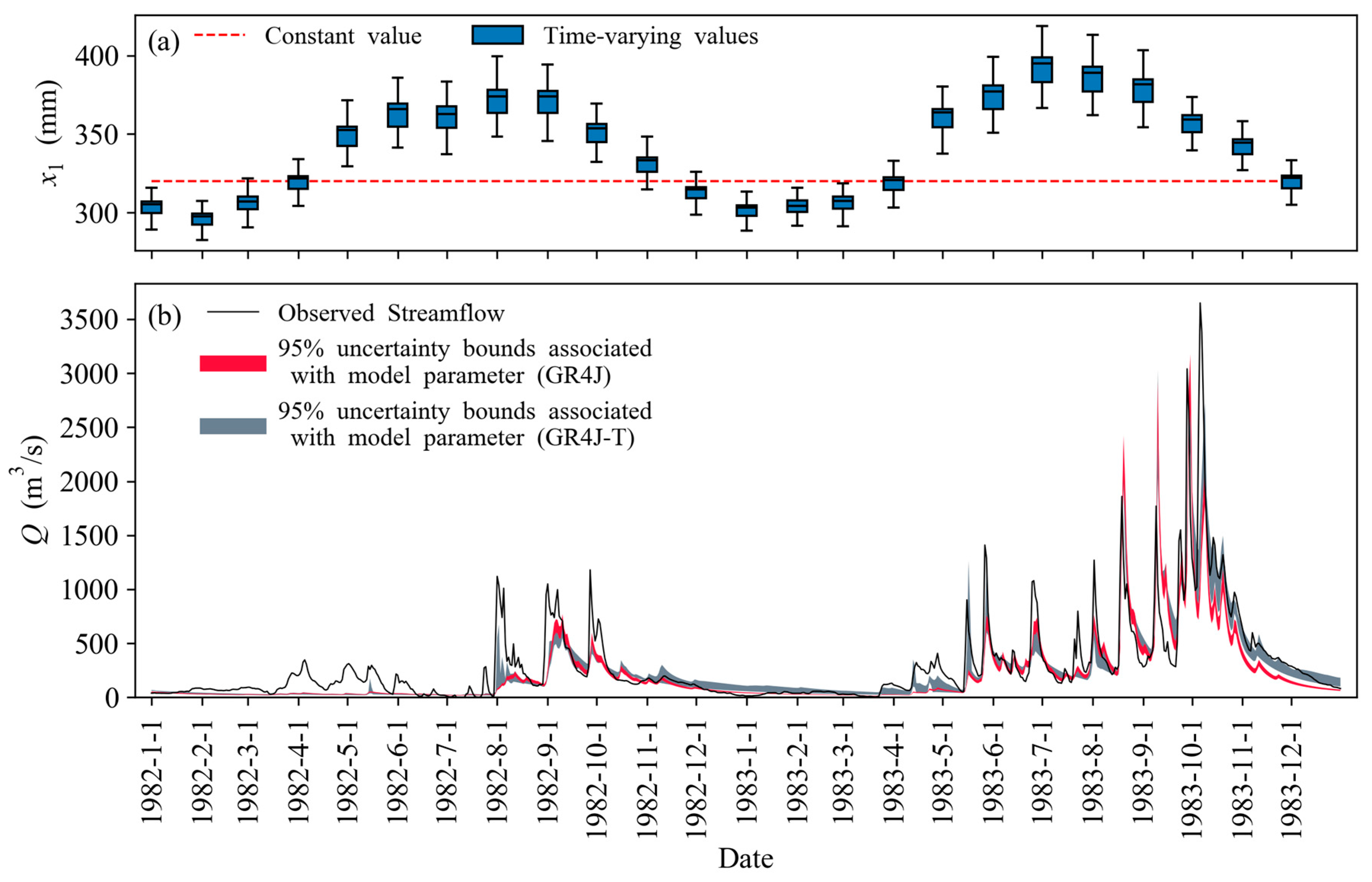
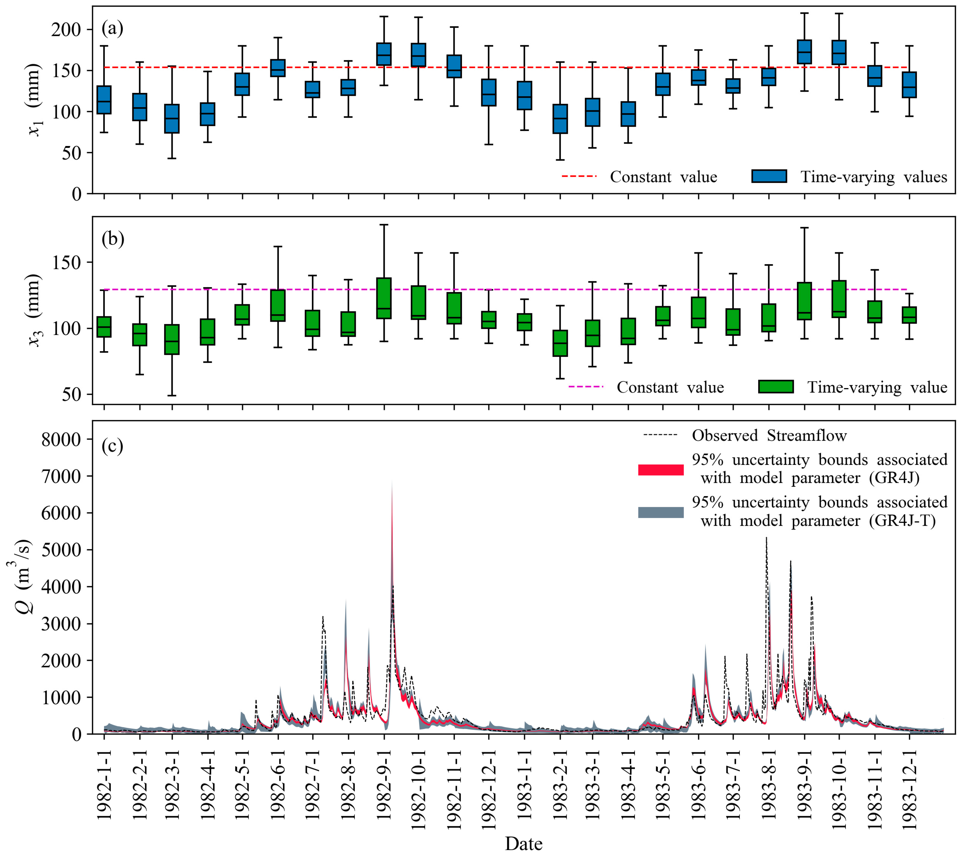
The observed streamflow and the uncertainty bounds associated with model parameter for both models during part of SP1 (1982–1983) are presented in Figure 6 (for Weihe Basin) and Figure 7 (for Tuojiang Basin) for an illustration purpose. The uncertainty bounds associated with model parameter were calculated as follows [59]. For both the GR4J and GR4J-T model, the streamflow simulation for a certain sub-period was repeated using the 5000 parameter sets, and 5000 simulated hydrographs were therefore obtained. Then the likelihood value of each parameter set was assigned to the respective simulated hydrograph. At each time step of the simulation, the posterior distributions of simulated streamflow can be calculated based on the 5000 simulated streamflow and the corresponding likelihood values. The upper and lower uncertainty bounds are here defined as the 2.5% and 97.5% quantiles of the posterior distribution, respectively. Then the 95% predictive uncertainty bounds associated with model parameter for both models were obtained. More detail of the calculation of the predictive uncertainty bounds can be found in the work of Blasone et al. [59]. The red and grey shaded areas indicate the prediction uncertainty associated with the GR4J model and GR4J-T model, respectively. It can be found that most parts of the observed streamflow series lie within the uncertainty bounds for both models, indicating a good simulation performance. In addition, the original GR4J model tends to underestimate the low flows in Weihe Basin, as presented in Figure 6b, where the simulated streamflow series is constantly lower than the observed in November of 1983. However, the average relative bandwidth of the uncertainty bounds associated with the GR4J-T model is wider, which indicates a higher parameter uncertainty. This agrees with the finding of Wallner and Haberlandt [25], who showed that time-varying model parameters can improve the model performance at the cost of possible growth in parameter uncertainty. The growth in parameter uncertainty may also relate to the choice of the external time-varying covariates when applying time-varying parameter, which may be an interesting topic that deserves further exploration.

Figure 6a presents the constant value of the parameter $x_1$ and its temporal dynamic when treated as time-varying for Weihe Basin during part of SP1 (1982–1983). The constant value was obtained from the KGE-best parameter set of the GR4J model, while the temporal dynamic of $x_{1,t}$ is presented in the form of boxplot using the 5000 resultant parameter sets of the GR4J-T model. It can be seen that the time-varying parameter $x_{1,t}$ increases in the growing season and decreases as the dormant season begins, with its values around the constant value of the parameter $x_1$. The case is the same for the parameter $x_1$ and $x_3$ in Tuojiang Basin, as shown in Figure 7a,b.

The increased value of the parameter $x_1$ during the growing season indicates larger catchment storage (e.g., interception) and, therefore, a weaker response of the watershed to precipitation inputs. As a result, the same hydrological inputs of precipitation may lead to less streamflow, therefore lower runoff ratio when compared to the dormant season. Likewise, the relatively low value of the parameter $x_1$ during the dormant season may lead to a stronger response to the precipitation inputs and may help to reduce the possibility to underestimate the low flow, as mentioned above. The parameter $x_3$, which controls the routing storage of GR4J model, shows a similar trend with $x_1$ in the case of Tuojiang. Similarly, the relatively low values of the parameter $x_3$ during dormant season, could contribute to a more rapid hydrological response and therefore a better representation of the low flow.

The improved streamflow simulation performance can be attributed to: (1) the dynamics in model parameter, which may help to compensate the possible deficiency of model structure, (2) the increased degree of freedom of model parameters. For the GR4J-T model applied in Weihe Basin, the number of parameters that required calibration is 7. The trade-off between a simple model structure and good model performance could be an interesting topic that deserves further researches, especially under changing environments.

4.4. Parameter Transferability of the GR4J and GR4J-T Model

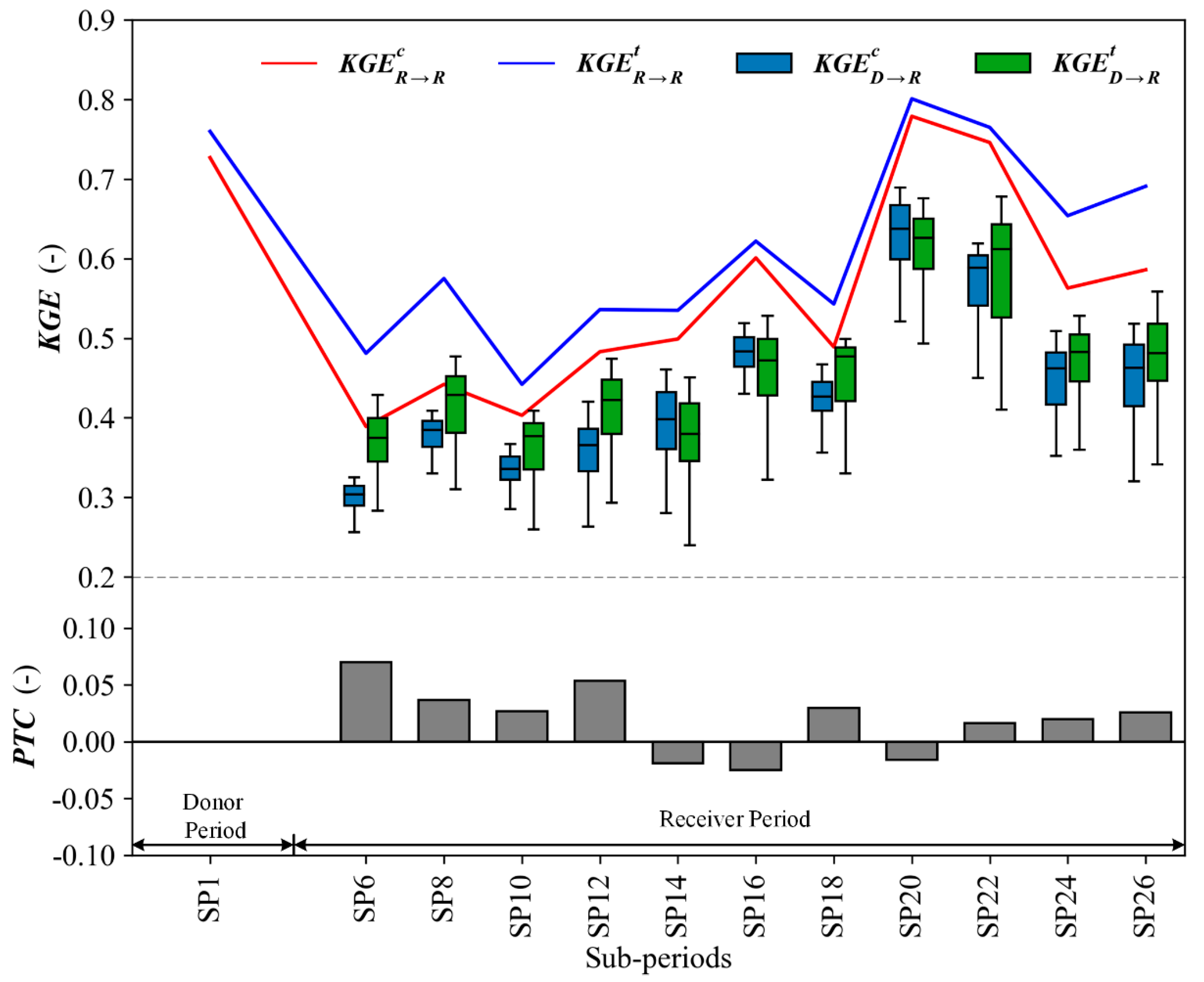
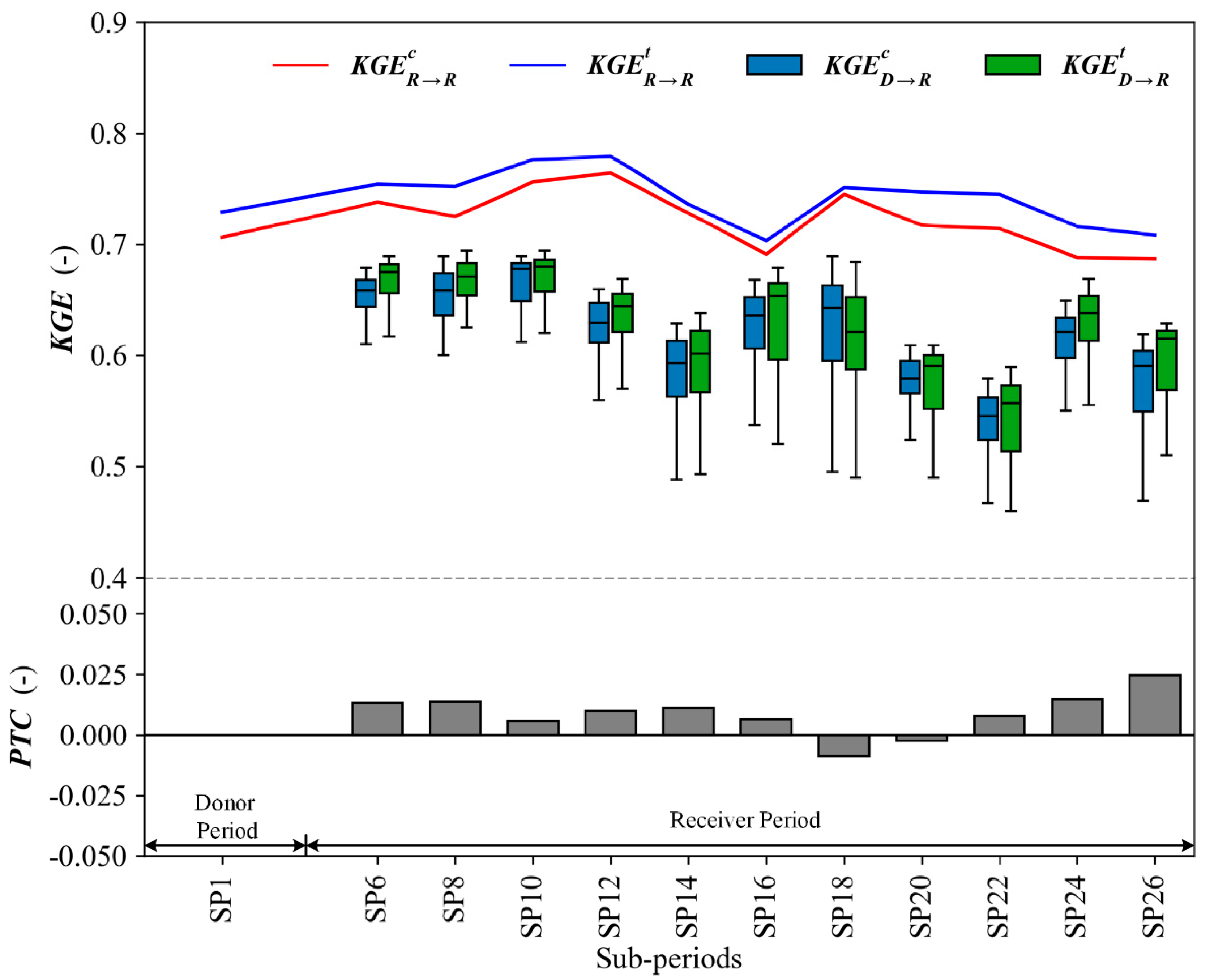
To test the parameter transferability of the GR4J and GR4J-T Model, the abovementioned 5000 parameter sets obtained from each sub-period (donor period) were then validated at its independent sub-periods (receiver periods). For example, Figure 8 compares the streamflow simulation performance of the GR4J model and GR4J-T model under 10 different sub-periods using parameter sets obtained from SP1 in Weihe Basin. The corresponding PTC criteria are also presented. As a reference, the red solid line represents the highest value of KGE ($KG{E}_{R\to R}^c$) achieved by the original GR4J model using parameter from each receiver period, while the blue solid line for the GR4J-T model ($KG{E}_{R\to R}^t$). The blue boxes represent the KGE values ($KG{E}_{D\to R}^c$) achieved by the original GR4J model using the 5000 parameter sets obtained from SP1, and the green boxes represent those of the GR4J-T model ($KG{E}_{D\to R}^t$). It is clear that when parameter sets were transferred from the donor period to the receiver periods, the model performance significantly decreased for both the GR4J model and GR4J model. However, the maximum value of the green boxes ($KG{E}_{D\to R}^t$) is constantly higher than those of the blue boxes ($KG{E}_{D\to R}^c$), as shown in Figure 8. Besides, the PTC criteria, which is the difference between the average value of KGE achieved using 5000 parameter sets by both models over each receiver period (see Equation (6)), is above 0 in most cases, which indicates a better temporal transferability of the GR4J-T model. The case is the same for Tuojiang Basin (see Figure 9), though the corresponding PTC values are quite close to 0.

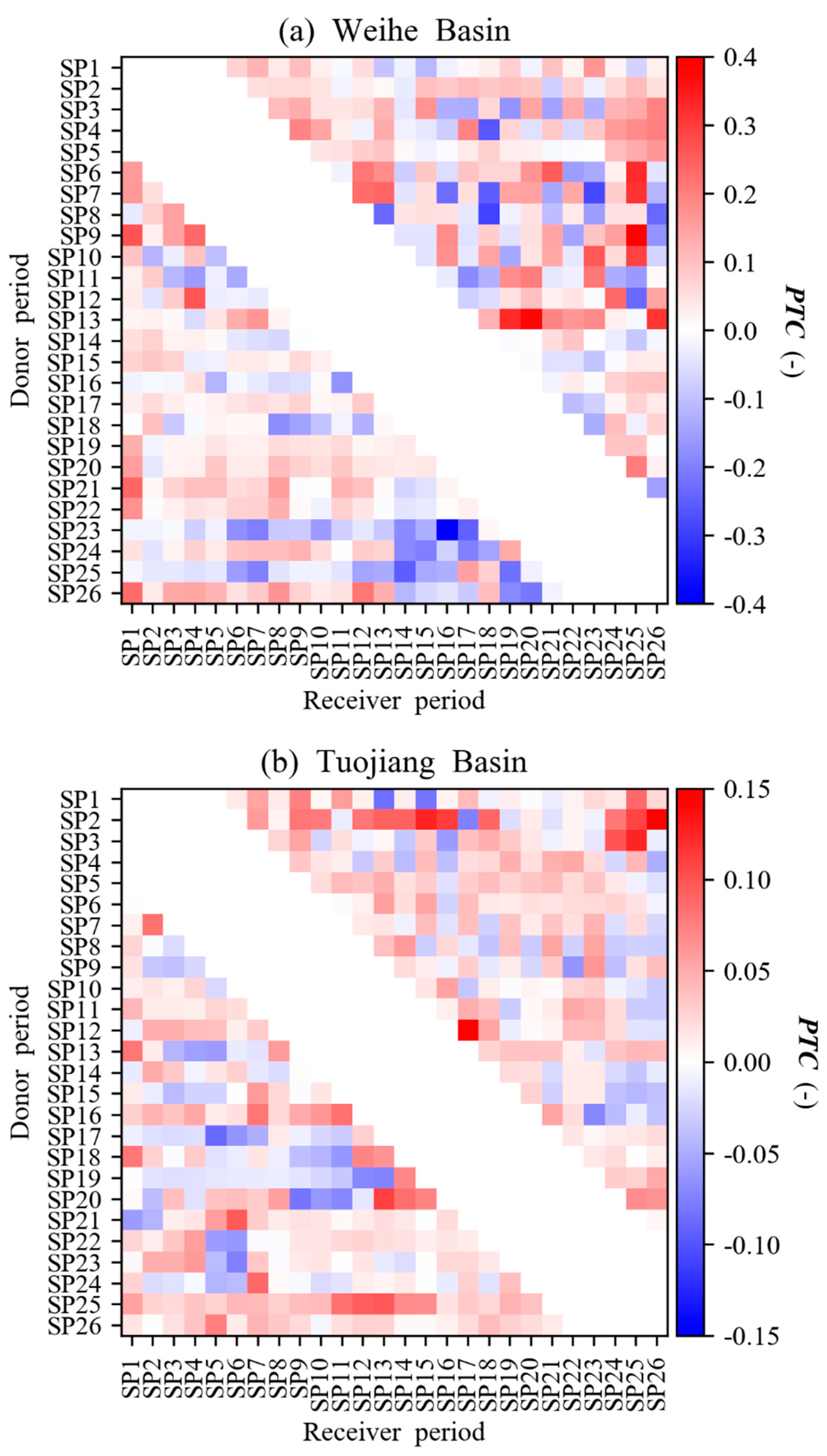
To comprehensively compare the temporal transferability of the constant parameter and the time-varying parameter, the PTC criteria for every possible case is also presented in Figure 10. The blank area indicates the cases where the transferability test is inapplicable (e.g., between adjacent sub-periods or among sub-periods that overlap each other). The labels on the y-axis indicate the 26 donor periods while the labels on the x-axis indicate the receiver periods. Each cell in the figure stands for a transferability test and its color represents the corresponding PTC value. The red cells, indicating positive PTC values, stands for the cases where the GR4J-T model shows a better temporal transferability over the GR4J model, while the blue cells are in the opposite cases. It is clear that the PTC criteria have a positive value in most cases. This further demonstrates that the GR4J-T model has advantage in term of temporal transferability over the original GR4J model.

Note that the loss in model performance when the model parameter was transferred among sub-period with different climate and watershed conditions is inevitable even for the hydrological model with time-varying parameter. Here, it was proven that a better transferability can be achieved under changing environments when applying the time-varying parameter. Though in practice, applying the time-varying parameter is not an easy job, as a more complicated calibration procedure is necessary. However, it is still worth identifying the sensitive parameter and find out how it may change over time, which may help to improve the model structure and to provide new sights for better understanding the hydrological processes.

5. Conclusions

This study investigated the parameter transferability under changing environments of the original GR4J model and its modified version, in which the parameter was allowed to vary over time. To set up the GR4J model with the time-varying parameter, a sensitivity analysis was applied to identify the most sensitive parameter, which was then treated as time-varying and assumed to be a function of several external covariates. Both models were calibrated and validated in a series of sub-periods with different climatic and watershed conditions. The investigation was carried out for Weihe Basin and Tuojiang Basin in western China. The main findings of this study are as follows:

(1) A better streamflow simulation performance in terms of the KGE criteria was achieved by the GR4J model with time-varying parameters ($x_1$ for Weihe Basin, $x_1$ and $x_3$ for Tuojiang Basin) during most calibration sub-periods for both basins, though at the cost of slight growth in parameter uncertainty,

(2) The GR4J model with time-varying parameter shows a better transferability among sub-periods with different climate and watershed conditions when compared to the original GR4J model for both basins.

Although the time-invariance of model parameters is one of the basic criteria of a high-quality hydrologic model, very few (if any) models can achieve this due to their inherent limitations. Numerous previous studies have proved that hydrological models with time-varying parameters can achieve a better streamflow simulation performance during the calibration period. This study further demonstrates the advantage of the GR4J model with time-varying parameter in terms of temporal transferability among different sub-periods. This may provide new insights for improving the structure of existing hydrological models and for building new models.

Considering the availability of the dataset for both basins, only six climate-related covariates (P₁, P₂, P_3, PET₁, PET_2, and PET₃) and 2 watershed-related covariates (NDVI₀ and NDVI₁) were accounted for to describe the dynamic variation of the selected parameter. More covariates should be investigated in further researches. Besides, the key factor that leads to the alternation in flow regimes also differs for different catchments. Thus, more emphases should be placed on the careful identification of proper external covariates when applying time-varying parameter.

References

- Duan, Q.; Sorooshian, S.; Gupta, V.K. Effective and efficient global optimization for conceptual rain-runoff models. Water Resour. Res. 1992, 28, 1015–1031. [Google Scholar] [CrossRef]
- Vrugt, J.A.; Gupta, H.V.; Bouten, W.; Sorooshian, S. A Shuffled Complex Evolution Metropolis algorithm for optimization and uncertainty assessment of hydrologic model parameters. Water Resour. Res. 2003, 39, 1201. [Google Scholar] [CrossRef]
- Milly, P.; Betancourt, J.; Falkenmark, M.; Hirsch, R.M.; Kundzewicz, Z.W.; Lettenmaier, D.P.; Stouffer, R.J. Stationarity is Dead: Whither Water Management. Science 2008, 319, 573–574. [Google Scholar] [CrossRef]
- Vansteenkiste, T.; Tavakoli, M.; Ntegeka, V.; De Smedt, F.; Batelaan, O.; Pereira, F.; Willems, P. Intercomparison of hydrological model structures and calibration approaches in climate scenario impact projections. J. Hydrol. 2014, 519, 743–755. [Google Scholar] [CrossRef]
- Merz, R.; Parajka, J.; Blöschl, G. Time stability of catchment model parameters: Implications for climate impact analyses. Water Resour. Res. 2011, 47, w02531. [Google Scholar] [CrossRef]
- Saft, M.; Peel, M.C.; Western, A.W.; Perraud, J.; Zhang, L. Bias in streamflow projections due to climate-induced shifts in catchment response. Geophys. Res. Lett. 2016, 43, 1574–1581. [Google Scholar] [CrossRef]
- Xu, C.; Chen, H.; Guo, S. Hydrological Modeling in a Changing Environment: Issues and Challenges. J. Water Resour. Res. 2013, 2, 85–95. [Google Scholar] [CrossRef]
- Silberstein, R.P.; Aryal, S.K.; Braccia, M.; Durrant, J. Rainfall-runoff model performance suggests a change in flow regime and possible lack of catchment resilience. In Proceedings of the 20th International Congress on Modelling and Simulation (MODSIM2013), Adelaide, Australia, 1–6 December 2013; pp. 2409–2415. [Google Scholar]
- Omer, A.; Wang, W.G.; Basheer, A.K.; Yong, B. Integrated assessment of the impacts of climate variability and anthropogenic activities on river runoff: A case study in the Hutuo River Basin, China. Hydrol. Res. 2017, 48, 416–430. [Google Scholar] [CrossRef]
- Le Lay, M.; Galle, S.; Saulnier, G.M.; Braud, I. Exploring the relationship between hydroclimatic stationarity and rainfall-runoff model parameter stability: A case study in West Africa. Water Resour. Res. 2007, 43, 7. [Google Scholar] [CrossRef]
- Choi, H.T.; Beven, K. Multi-period and multi-criteria model conditioning to reduce prediction uncertainty in an application of TOPMODEL within the GLUE framework. J. Hydrol. 2007, 332, 316–336. [Google Scholar] [CrossRef]
- Broderick, C.; Matthews, T.; Wilby, R.L.; Bastola, S.; Murphy, C. Transferability of hydrological models and ensemble averaging methods between contrasting climatic periods. Water Resour. Res. 2016, 52, 8343–8373. [Google Scholar] [CrossRef] [Green Version]
- Singh, R.; van Werkhoven, K.; Wagener, T. Hydrological impacts of climate change in gauged and ungauged watersheds of the Olifants basin: A trading-space-for-time approach. Hydrol. Sci. J. 2014, 59, 29–55. [Google Scholar] [CrossRef]
- Lacombe, G.; Ribolzi, O.; de Rouw, A.; Pierret, A.; Latsachak, K.; Silvera, N.; Pham Dinh, R.; Orange, D.; Janeau, J.; Soulileuth, B.; et al. Contradictory hydrological impacts of afforestation in the humid tropics evidenced by long-term field monitoring and simulation modelling. Hydrol. Earth Syst. Sci. 2016, 20, 2691–2704. [Google Scholar] [CrossRef] [Green Version]
- De Vos, N.J.; Rientjes, T.H.M.; Gupta, H.V. Diagnostic evaluation of conceptual rainfall-runoff models using temporal clustering. Hydrol. Process. 2010, 24, 2840–2850. [Google Scholar] [CrossRef]
- Gharari, S.; Hrachowitz, M.; Fenicia, F.; Savenije, H.H.G. An approach to identify time consistent model parameters: Sub-period calibration. Hydrol. Earth Syst. Sci. 2013, 17, 149–161. [Google Scholar] [CrossRef]
- Guo, D.; Johnson, F.; Marshall, L. Assessing the Potential Robustness of Conceptual Rainfall-Runoff Models Under a Changing Climate. Water Resour. Res. 2018, 54, 5030–5049. [Google Scholar] [CrossRef]
- Ekström, M.; Gutmann, E.D.; Wilby, R.L.; Tye, M.R.; Kirono, D.G.C. Robustness of hydroclimate metrics for climate change impact research. Wiley Interdiscip. Rev. Water 2018, 5, e1288. [Google Scholar] [CrossRef]
- Motavita, D.F.; Chow, R.; Guthke, A.; Nowak, W. The comprehensive differential split-sample test: A stress-test for hydrological model robustness under climate variability. J. Hydrol. 2019, 573, 501–515. [Google Scholar] [CrossRef]
- Fowler, K.; Coxon, G.; Freer, J.; Peel, M.; Wagener, T.; Western, A.; Woods, R.; Zhang, L. Simulating Runoff Under Changing Climatic Conditions: A Framework for Model Improvement. Water Resour. Res. 2018, 54, 9812–9832. [Google Scholar] [CrossRef] [Green Version]
- Vormoor, K.; Heistermann, M.; Bronstert, A.; Lawrence, D. Hydrological model parameter (in) stability-“crash testing” the HBV model under contrasting flood seasonality conditions. Hydrol. Sci. J. 2018, 63, 991–1007. [Google Scholar] [CrossRef]
- Kim, S.S.H.; Hughes, J.D.; Chen, J.; Dutta, D.; Vaze, J. Determining probability distributions of parameter performances for time-series model calibration: A river system trial. J. Hydrol. 2015, 530, 361–371. [Google Scholar] [CrossRef]
- Paik, K.; Kim, J.H.; Kim, H.S.; Lee, D.R. A conceptual rainfall-runoff model considering seasonal variation. Hydrol. Process. 2005, 19, 3837–3850. [Google Scholar] [CrossRef]
- Du, J.; Rui, H.; Zuo, T.; Li, Q.; Zheng, D.; Chen, A.; Xu, Y.; Xu, C.Y. Hydrological Simulation by SWAT Model with Fixed and Varied Parameterization Approaches Under Land Use Change. Water Resour. Manag. 2013, 27, 2823–2838. [Google Scholar] [CrossRef]
- Wallner, M.; Haberlandt, U. Non-stationary hydrological model parameters: A framework based on SOM-B. Hydrol. Process. 2015, 29, 3145–3161. [Google Scholar] [CrossRef]
- Pathiraja, S.; Marshall, L.; Sharma, A.; Moradkhani, H. Hydrologic modeling in dynamic catchments: A data assimilation approach. Water Resour. Res. 2016, 52, 3350–3372. [Google Scholar] [CrossRef] [Green Version]
- Westra, S.; Thyer, M.; Leonard, M.; Kavetski, D.; Lambert, M. A strategy for diagnosing and interpreting hydrological model nonstationarity. Water Resour. Res. 2014, 50, 5090–5113. [Google Scholar] [CrossRef] [Green Version]
- Deng, C.; Liu, P.; Wang, W.; Shao, Q.; Wang, D. Modelling time-variant parameters of a two-parameter monthly water balance model. J. Hydrol. 2019, 573, 918–936. [Google Scholar] [CrossRef]
- Sadegh, M.; AghaKouchak, A.; Flores, A.; Mallakpour, I.; Nikoo, M.R. A Multi-Model Nonstationary Rainfall-Runoff Modeling Framework: Analysis and Toolbox. Water Resour. Manag. 2019, 33, 3011–3024. [Google Scholar] [CrossRef]
- Pathiraja, S.; Anghileri, D.; Burlando, P.; Sharma, A.; Marshall, L.; Moradkhani, H. Time-varying parameter models for catchments with land use change: The importance of model structure. Hydrol. Earth Syst. Sci. 2018, 22, 2903–2919. [Google Scholar] [CrossRef]
- Xiong, M.; Liu, P.; Cheng, L.; Deng, C.; Gui, Z.; Zhang, X.; Liu, Y. Identifying time-varying hydrological model parameters to improve simulation efficiency by the ensemble Kalman filter: A joint assimilation of streamflow and actual evapotranspiration. J. Hydrol. 2019, 568, 758–768. [Google Scholar] [CrossRef]
- Rabassa, P.; Beck, C. Superstatistical analysis of sea-level fluctuations. Phys. A Stat. Mech. Its Appl. 2015, 417, 18–28. [Google Scholar] [CrossRef] [Green Version]
- Yalcin, G.C.; Rabassa, P.; Beck, C. Extreme event statistics of daily rainfall: Dynamical systems approach. J. Phys. A Math. Theor. 2016, 49, 154001. [Google Scholar] [CrossRef]
- Perrin, C.; Michel, C.; Andréassian, V. Improvement of a parsimonious model for streamflow simulation. J. Hydrol. 2003, 279, 275–289. [Google Scholar] [CrossRef]
- Sobol, I.M. Global sensitivity indices for nonlinear mathematical models and their Monte Carlo estimates. Math. Comput. Simul. 2001, 55, 271–280. [Google Scholar] [CrossRef]
- Herman, J.D.; Reed, P.M.; Wagener, T. Time-varying sensitivity analysis clarifies the effects of watershed model formulation on model behavior. Water Resour. Res. 2013, 49, 1400–1414. [Google Scholar] [CrossRef]
- Patil, S.D.; Stieglitz, M. Comparing spatial and temporal transferability of hydrological model parameters. J. Hydrol. 2015, 525, 409–417. [Google Scholar] [CrossRef] [Green Version]
- Arsenault, R.; Brissette, F.; Martel, J. The hazards of split-sample validation in hydrological model calibration. J. Hydrol. 2018, 566, 346–362. [Google Scholar] [CrossRef]
- Coron, L.; Andréassian, V.; Perrin, C.; Lerat, J.; Vaze, J.; Bourqui, M.; Hendrickx, F. Crash testing hydrological models in contrasted climate conditions: An experiment on 216 Australian catchments. Water Resour. Res. 2012, 48, w05552. [Google Scholar] [CrossRef]
- Coron, L.; Andréassian, V.; Perrin, C.; Bourqui, M.; Hendrickx, F. On the lack of robustness of hydrologic models regarding water balance simulation: A diagnostic approach applied to three models of increasing complexity on 20 mountainous catchments. Hydrol. Earth Syst. Sci. 2014, 18, 727–746. [Google Scholar] [CrossRef]
- Gupta, H.V.; Kling, H.; Yilmaz, K.K.; Martinez, G.F. Decomposition of the mean squared error and NSE performance criteria: Implications for improving hydrological modelling. J. Hydrol. 2009, 377, 80–91. [Google Scholar] [CrossRef] [Green Version]
- Feyen, L.; Vrugt, J.A.; Nualláin, B.Ó.; van der Knijff, J.; De Roo, A. Parameter optimisation and uncertainty assessment for large-scale streamflow simulation with the LISFLOOD model. J. Hydrol. 2007, 332, 276–289. [Google Scholar] [CrossRef] [Green Version]
- Metropolis, N.; Rosenbluth, A.W.; Rosenbluth, M.N.; Teller, A.H.; Teller, E. Equation of state calculations by fast computing machines. J. Chem. Phys. 1953, 21, 1087–1092. [Google Scholar] [CrossRef]
- Hastings, W.K. Monte Carlo Sampling Methods Using Markov Chains and Their Applications; Oxford University Press: Oxford, UK, 1970. [Google Scholar]
- Ajami, N.K.; Duan, Q.; Sorooshian, S. An integrated hydrologic Bayesian multimodel combination framework: Confronting input, parameter, and model structural uncertainty in hydrologic prediction. Water Resour. Res. 2007, 43, w01403. [Google Scholar] [CrossRef]
- Gelman, A.; Rubin, D.B. Inference from iterative simulation using multiple sequences. Stat. Sci. 1992, 7, 457–472. [Google Scholar] [CrossRef]
- Li, S.; Xiong, L.; Li, H.; Leung, L.R.; Demissie, Y. Attributing runoff changes to climate variability and human activities: Uncertainty analysis using four monthly water balance models. Stoch. Environ. Res. Risk Assess. 2015, 30, 251–269. [Google Scholar] [CrossRef]
- Xiong, L.; Du, T.; Xu, C.Y.; Guo, S.; Jiang, C.; Gippel, C.J. Non-Stationary Annual Maximum Flood Frequency Analysis Using the Norming Constants Method to Consider Non-Stationarity in the Annual Daily Flow Series. Water Resour. Manag. 2015, 29, 3615–3633. [Google Scholar] [CrossRef]
- Jiang, C.; Xiong, L.; Wang, D.; Liu, P.; Guo, S.; Xu, C.Y. Separating the impacts of climate change and human activities on runoff using the Budyko-type equations with time-varying parameters. J. Hydrol. 2015, 522, 326–338. [Google Scholar] [CrossRef]
- Zou, L.; Xia, J.; She, D. Analysis of Impacts of Climate Change and Human Activities on Hydrological Drought: A Case Study in the Wei River Basin, China. Water Resour. Manag. 2018, 32, 1421–1438. [Google Scholar] [CrossRef]
- Su, X.L.; Kang, S.Z.; Wei, X.M.; Xing, D.W.; Cao, H. Impact of climate change and human activity on the runoff of Wei River basin to the Yellow River. J. Northwest A F Univ. (Nat. Sci. Ed.) 2007, 35, 153–159. [Google Scholar]
- Luan, X.; Wu, P.; Sun, S.; Li, X.; Wang, Y.; Gao, X. Impact of Land Use Change on Hydrologic Processes in a Large Plain Irrigation District. Water Resour. Manag. 2018, 32, 3203–3217. [Google Scholar] [CrossRef]
- National Meteorological Information Center of China. Available online: http://data.cma.cn/ (accessed on 30 July 2019).
- Blaney, H.F.; Criddle, W.D. Determining Consumptive Use and Irrigation Water Requirements, USDA Technical Bulletin 1275; US Department of Agriculture: Washington, DC, USA, 1962.
- Fensholt, R.; Rasmussen, K. Analysis of trends in the Sahelian ‘rain-use efficiency’ using GIMMS NDVI, RFE and GPCP rainfall data. Remote Sens. Environ. 2011, 115, 438–451. [Google Scholar] [CrossRef]
- Fensholt, R.; Proud, S.R. Evaluation of Earth Observation based global long-term vegetation trends—Comparing GIMMS and MODIS global NDVI time series. Remote Sens. Environ. 2012, 119, 131–147. [Google Scholar] [CrossRef]
- Mann, H.B. Non-parametric tests against trend. Econometrica 1945, 13, 245–259. [Google Scholar] [CrossRef]
- Kendall, M.G. Rank Correlation Measures; Charles Griffin: London, UK, 1975. [Google Scholar]
- Blasone, R.; Madsen, H.; Rosbjerg, D. Uncertainty assessment of integrated distributed hydrological models using GLUE with Markov chain Monte Carlo sampling. J. Hydrol. 2008, 353, 18–32. [Google Scholar] [CrossRef] [Green Version]
Figure 1.
Illustration of the generalized split-sample test (GSST) procedure (example with 15 years available and 5-year subperiods). (Adapted from the work of Coron et al. [40]).
Figure 2.
Location of Weihe Basin and Tuojiang Basin in China and the meteorological and hydrological gauges.
Figure 3.
Relative long-term hydro-meteorological variability of (a) precipitation (P), (b) potential evapotranspiration (PET), (c) runoff (Q), and (d) runoff ratio (RR) over Weihe Basin and Tuojiang Basin.
Figure 4.
Monthly total-order sensitivity indices of GR4J parameters for (a) Weihe Basin and (b) Tuojiang Basin. For each basin, the left panel and the right panel share the same sensitivity indices, but they are sorted by monthly total precipitation (left) and monthly streamflow (right), respectively.
Figure 5.
Spearman rank correlation coefficient between monthly covariates and monthly runoff ratio (RR) for Weihe Basin and Tuojiang Basin for the whole period (1981–2010).
Figure 6.
Temporal comparison of (a) the values of the parameter and (b) the simulated daily streamflow of the GR4J model and the GR4J-T model for Weihe Basin during SP1 (only the period from 1 January 1982 to 31 December 1983 are presented here). The uncertainty bounds associated with model parameter are derived from the streamflow simulation results using the corresponding 5000 parameter sets.
Figure 7.
Temporal comparison of the values of the parameter (a) and (b) , and (c) the simulated daily streamflow of the GR4J model and the GR4J-T model for Tuojiang Basin during SP1 (only the period from 1 January 1982 to 31 December 1983 are presented here). The uncertainty bounds associated with model parameter are derived from the streamflow simulation results using the corresponding 5000 parameter sets.
Figure 8.
Comparison of streamflow simulation performance in terms of KGE when parameter sets calibrated during P1 are transferred to other sub-periods (SP6–SP26) for the GR4J model and the GR4J-T model in Weihe Basin. The boxplots represent the KGE values using the 5000 parameter sets obtained from SP1. The PTC values indicate the difference of the average simulation performance between the GR4J model and the GR4J-T model during the validation procedure.
Figure 9.
Comparison of streamflow simulation performance in terms of KGE when parameter sets calibrated during P1 are transferred to other sub-periods (SP6–SP26) for the GR4J model and the GR4J-T model in Tuojiang Basin.
Figure 10.
PTC values of the parameter transferability test for (a) Weihe Basin and (b) Tuojiang Basin.