Assessment of Water Resources Management Strategy Under Different Evolutionary Optimization Techniques

Abstract

Competitive optimization techniques have been developed to address the complexity of integrated water resources management (IWRM) modelling; however, model adaptation due to changing environments is still a challenge. In this paper we employ multi-variable techniques to increase confidence in model-driven decision-making scenarios. Here, water reservoir management was assessed using two evolutionary algorithm (EA) techniques, the epsilon-dominance-driven self-adaptive evolutionary algorithm (ε-DSEA) and the Borg multi-objective evolutionary algorithm (MOEA). Many objective scenarios were evaluated to manage flood risk, hydropower generation, water supply, and release sequences over three decades. Computationally, the ε-DSEA’s results are generally reliable, robust, effective and efficient when compared directly with the Borg MOEA but both provide decision support model outputs of value.

1. Introduction

Water resource management problems (i.e., surface and groundwater) are complex due to their non-linear, dynamic, multimodal properties that need robust methods to solve, such as optimization algorithms [1] based on evolutionary algorithms (EAs) inspired from evolution and the natural selection of species [2,3]. Many of these have been proposed by researchers with different techniques, such as: the non-dominated sorting genetic algorithm (NSGA II) [4], multi-objective evolutionary algorithm based on decomposition (MOEA/D) [5], indicator-based evolutionary algorithm (IBEA) [6] and differential evolution (DE) [7]. Furthermore, approaches based on swarm intelligence include particle swarm optimization (PSO) [8] and ant colony optimization (ACO) [9] while the annealing process in metallurgy inspired simulated annealing (SA) [10]. A review of EAs and other metaheuristic algorithms and their applications can be found in [11,12]. Examples using these techniques for solving water resources management problems include Hurford et al., [13], and others [14,15,16,17] using ε-NSGA-II, MOEA/D, Borg MOEA and NSGA-II, respectively to optimize reservoir management strategy based on multidisciplinary objectives like flood control, hydropower generation, and water supply.

Benchmark functions such as DTLZ and WFG series were often used in comparative studies to assess algorithms’ performance, as in [18,19,20,21], however they consider forward and easy to solve versus real-world problems [22]. These algorithms often have many parameters that require calibration, which has a major impact on computational performance and optimal achievement [23,24]. Karafotias et al., [25] presented a review of the approaches for the calibration and control of parameters. There are two types of EA parameter-setting problems categorised as (a) parameter tuning and (b) parameter control. Parameter tuning relates to the initial values of some parameters that are set before executing the algorithm. Parameter control involves adjusting values during the run time [26].

Parameter tuning is applied to parameters such as population size, mutation and crossover rate, and has been discussed in the literature and recommended values proposed [25]. However, some of the parameters can vary widely and generally need extensive trials to find suitable values for a particular problem. For example, the distribution index for the simulated binary crossover (SBX) operator may vary between 0 and 500 [27]. Similarly, Reynoso-Meza et al., [28] concluded from experimental studies on multi-objective optimization problems that the value of the step size for the differential evolution (DE) operator is case sensitive. It is difficult to set default values for all problems. Parameter control is more important than parameter tuning in genetic algorithms (which directly affect the algorithms’ performance) [29], however, these parameters have received less attention in the literature [25]. These issues reduce the confidence of decision makers to use modelled EA results [1]. For example, Ishibuchi et al., [21] demonstrates that algorithms’ optimality behaviour may change under different problems’ environments, based on experimental studies on test benchmark functions. Nevertheless, the need of EA models capable to adapt with such a problematic is evident.

In this article, a novel approach ε-DSEA (epsilon-dominance-driven self-adaptive evolutionary algorithm) is presented using a range of novel techniques including: (i) Diversity expansion; (ii) Self-adaptation of the control parameters of recombination operators; (iii) Exploration extension; and (iv) Virtual dominance archive. The algorithm’s performance was investigated using a constrained real-world regional water resources management problem. A comparative analysis with Borg MOEA [30] was utilized as the Borg MOEA has superior reliability when compared with a range of robust published algorithms [18,31].

The key properties that define the comparison are: (i) Reliability, which refers to the replication and consistency of the best solutions achieved [32] (ii); Robustness, which relates the algorithms dependable performance in different problem environments [22]; (iii) Computational efficiency, i.e. the algorithm’s speed of convergence to the non-dominated solutions [33]; and (iv) Effectiveness, which refers to the closeness of the solutions achieved to the true Pareto-front and their distribution; and dominance front extension in objective space [34]. The outcome demonstrates the robustness of the proposed ε-DESA technique to maintain optimality achievement under different problem environments that may increase integrated water resources management (IWRM) decision makers’ confidence to adopt the EAs’ results.

2. Materials and Methods

2.1. Adopted Multi-Objective Optimization Approach

Commonly, real-word optimization problems have multiple objectives. A brief explanation of some of the key concepts associated with multi-objective optimization is provided here. An constrained multi-objective optimization problem may be described briefly as follows [35]

Minimize: F(x) = [f₁(x), ⋯, ⋯, ⋯f_M(x)]^T

(1)

$$\begin{gathered} \mathit{Subject}\mathit{to} g_i\left(x\right)\ge 0,\forall i\in n_g \\ {h}_j\left(x\right)=0,\forall j\in n_h \\ {x} \in X \end{gathered}$$

X ∈ Rⁿ is the decision space, i.e. X = [x^L, x^U] where x = [x₁, x₂, …, x_n]^T is the decision variable vector of dimension n; and x^L and x^U are the vectors of the lower and upper bounds on x, respectively. F(x) consists of M objective functions f_i : X →Z ∈ R^M, where i = 1, …, M, and Z is the objective space’s feasible region containing all decision variables in X that satisfy all constraints. The $g_i\left(x\right)$ and $h_j\left(x\right)$ represents the i^th of $n_g$ and j^th for $n_h$ inequality and equality constraints, respectively. For unconstraint problems, $n_g=n_h=\varnothing$, and Z = X [30].

The concept of Pareto-dominance [35,36,37] is used widely to characterise the solutions of multi-objective optimization problems, and superior solutions are said to dominate inferior solutions.

Thus:

• In a minimization problem, a vector u = (u₁, . . . , u_M)^T is said to dominate another vector v = (v₁, . . . , v_M)^T if u_i ≤ v_i for i = 1, . . . , M and u ≠ v. This property may be denoted as u ≺v.
• A feasible solution x∈ X is called a Pareto-optimal solution, if there is no alternative solution y∈ X such that F(y) ≺ F(x).
• The Pareto-optimal set, PS, is the union of all Pareto-optimal solutions, and may be defined as PS = {x ∈ X :$\nexists$y ∈ X, F(y) ≺ F(x)}.
• The Pareto-optimal front, PF, is the set comprising the Pareto-optimal solutions in the objective space. It may be expressed as PF = {F(x)|x ∈ PS}.

2.2. Details of Epsilon-Dominance-Driven Self-Adaptive Evolutionary Algorithm (ε-DSEA) Optimization Algorithm

The algorithm is based on the main principles of multi-objective evolutionary algorithms (MOEAs) e.g. recombination, mutation and dominance sorting. However, novel techniques are included to enhance the algorithm’s ability to handle the complexities of different problem environments. These techniques are:

• Diversity expansion to increase decision variables’ search space exploitation
• Self-adaptive operators’ parameters for parameters in process tuning
• Exploration extension for algorithm revival and stagnation coping
• Virtual dominance archive to improve diversity and convergence.

The algorithm employs six recombination operators having different evolving techniques for biological genetics process (e.g., crossover), which depend on chromosomes from the parent to generate new chromosomes. These operators are: simulated binary crossover (SBX) [27]; differential evolution (DE) [7]; parent-centric crossover (PCX) [38]; unimodal normal distribution crossover (UNDX) [39]; simplex crossover (SPX) [40]; and uniform mutation (UM) [41]. The corollary offspring (son) from these operators, excluding the UM, will mutate by polynomial mutation (PM) operator [42] to produce new generation set. Geetha and Kumaran [43] reviewed several crossover operators used in evolutionary algorithms. Here, the hyper-boxes (whose dimensions are equal to ε) sorting technique of objective search space [44], and non-dominated archive were employed as in [30,45,46].

2.2.1. Diversity Expansion

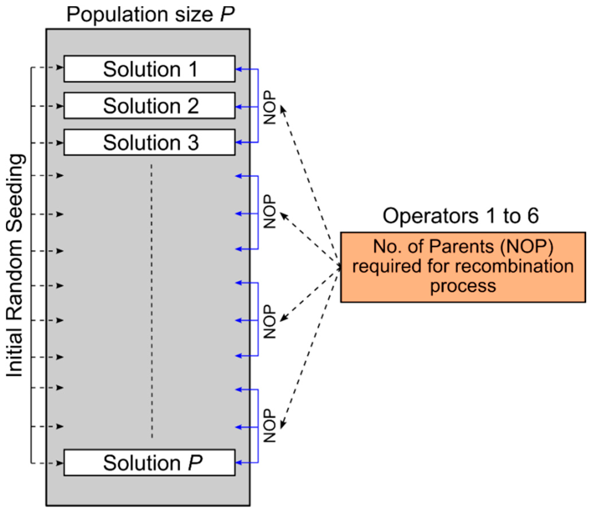
The search procedure in an optimization algorithm has two main components, exploration and exploitation. Evidence in the literature indicates the best results are achieved if exploration and exploitation are deployed preferentially in the early and latter stages of the search, respectively [47,48]. Accordingly, a procedure that safeguards diversity in the population at the start is incorporated in the proposed algorithm which employs all the available recombination operators at the initial stage. After the initial random seeding, the algorithm uses each recombination operator to generate new offspring, selecting parents from the entire population. If more parents are needed (e.g., in case of odd number of parents), they are selected from the population using a binary tournament selection. Figure 1 illustrates the procedure by which the parents are selected.

2.2.2. Self-Adaptive Mechanism and Formulae

In each generation, the recombination operators are selected on a competitive basis, according to the proportion of dominance solutions in the archive (NDS) contributed by each operator. Thus, the selection probabilities for the recombination operators are obtained as follows [30,49].

$${𝒫}_{\mathrm{i}}^{\mathrm{NDS}}=\frac{ND{S}_i+1}{{{\displaystyle \sum }}_{j=1}^{NRO}\left(ND{S}_j+1\right)}i,j=1,2,\dots NRO$$

(2)

where ${𝒫}_i^{NDS}$ is the probability of i^th recombination operator, NDS_i is the number of solutions in the archive contributed by the i^th recombination operator, NRO is the number of recombination operators; The constant 1.0 is used to avoid probability values of zero.

However, operator’s dominance achievement is sensitive to the relevant parameter setting. This problematic, (e.g., parameter control problem) was classified into three categories depending on the way the parameter variation is accomplished [26]: (a) deterministic, (b) adaptive, and (c) self-adaptive. Deterministic control is based on rules that are specified a priori [50,51]. In self-adaptive control, the parameters may be encoded to evolve in the genotype such that, for example, mutation and recombination are applied to the decision variables also [52,53], which extends the search space to cover the parameter values and consumes more time during the optimization processes [26]. The adaptive method (b) was considered more effective in solving complex problems, as a feedback from the optimization process is set to adjust parameter values during optimization progresses [26,54]. The aforementioned technique was adopted by many researchers to improve algorithms’ performance, as in [30,49,55,56,57], however none of these (and others) develop a self-adaptive technique that is sensitive to optimality achievement during evaluation progress [31].

The success of any operator depends on the chosen values of the parameters that directly affect its performance. Any operator may lead an algorithm to suboptimal solutions because of unsatisfactory parameter calibration. However, parameter calibration is extremely challenging. This difficulty provided the motivation for establishing a dynamic relationship between the values of the control parameters of the recombination operators and their relative effectiveness, to obviate the need for fine tuning. The efficiency of the optimization algorithm is thus improved by continuously seeking to improve the collective effectiveness of the recombination operators. In other words, the formulation developed herein allows the values of the control parameters of each recombination operator to improve adaptively based on the success of the recombination operator compared to the rest of the recombination operators.

Table 1. Parameters control formulae in epsilon-dominance-driven self-adaptive evolutionary algorithm (ε-DSEA).

Operator	Parameters	Domain	Adaptation Functions	Comments
SBX 1	$\eta$	[0, 100]	${𝒫}_i^{NDS}\times 100$	Distribution index
DE 2	CR F	[0.1,1.0] [0.5, 1.0]	$Max (0.1, {𝒫}_i^{NDS}{}_i)$ $0.5+\left({𝒫}_i^{NDS}/2\right)$	Crossover probability Step size
SPX 3	$\lambda$	[2.5, 3.5]	$2.5 +{𝒫}_i^{NDS}$	Expansion rate
PCX 4	${\sigma }_{\eta }$ ${\sigma }_{\zeta }$	[0.1, 0.3]	$0.1 +\left({𝒫}_i^{NDS}/5\right)$ $0.1 +\left({𝒫}_i^{NDS}/5\right)$	These parameters (standard deviations) control the spatial distribution of the offspring for PCX and UNDX
UNDX 4	${\mathsf{\sigma }}_{\mathsf{\zeta }}$ ${\mathsf{\sigma }}_{\mathsf{\eta }}$	[0.4, 0.6] [0.1, 0.35]$/\sqrt{L}$	$0.4 +\left({𝒫}_{\mathrm{i}}^{\mathrm{NDS}}/5\right)$ $\left[0.1 +\left({𝒫}_{\mathrm{i}}^{\mathrm{NDS}}/3\right)\right]/\sqrt{L}$

¹ Simulated Binary Crossover; ² Differential Evolution; ³ Simplex Crossover; ⁴ Parent-Centric Crossover; ⁵ Unimodal Normal Distribution Crossover

shows the lower and upper bounds of the operator control parameters. If an operator’s ability to contribute offspring to the dominance archive is decreased, its selection probability ${𝒫}_i^{NDS}$ will decrease according to Equation (2). In turn, the values of the relevant control parameter decrease and the recombination operator’s ability to contribute new offspring to the archive will improve.

It is worth noting that, initially, all the recombination operators have an equal selection probability (${𝒫}_i^{NDS}$) of 1/NRO. During the evaluation process the ${𝒫}_i^{NDS}$ value for any recombination operator changed along with its control parameters, according to its contribution in the dominance archive. If any recombination operator is relatively unsuccessful, its selection probability (${𝒫}_i^{NDS}$) and parameters controls will decrease. If the effectiveness of another recombination operator decreases, the selection probabilities of some or all the other recombination operators will increase with the values of their control parameters. In this way a dynamic equilibrium is maintained among the operators’ selection probabilities, which in turn regulates the operator control parameters. A set of formulae (equations) developed ensemble parameters’ tuning with the relevant dominance attainment. The parameters’ tuning domains (i.e., tuning range) were set based on default or recommended values suggested in the literature, and experimental investigation carried out on common test functions, as illustrated in Table 1.

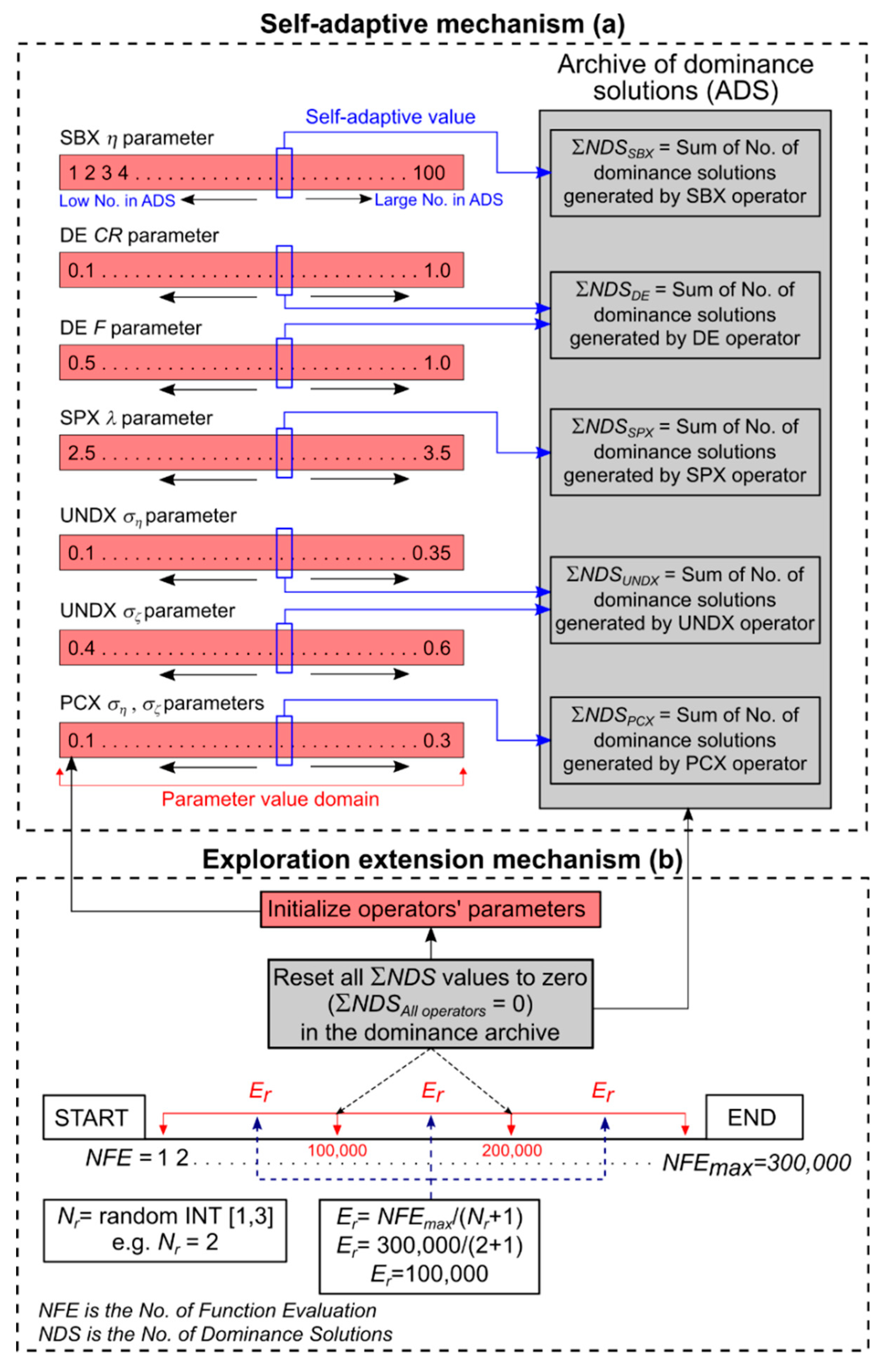
Figure 2a illustrates the relationships between operators’ dominance attainment and their control parameters values and shows how operators’ parameters auto-tuned according to the operator successful to produce non-dominated solutions in the dominance archive.

2.2.3. Exploration Extension Mechanism

This mechanism is based on initializing (resetting) all operators’ selection probabilities ${𝒫}_i^{NDS}$ uniformly to1/NRO. It aims to provide an equal opportunity for all the operators, by assessing the performance best on the most recent results. Otherwise, the previously successful operators with more solutions in the archive would continue to dominate based on past performance as dictated by Equation (2).

The number of resets depends on a random integer N_r such that $N_r$ ∈ ${\mathbb{N}}^{+}\in$ [1, 3]. When the algorithm starts, an N_r value is selected at random and the maximum permissible number of function evaluations NFE_max is divided by $N_r+1$ to determine the reset interval E_r. For example, if NFE_max = 300,000 and N_r = 2, the reset occurs at every E_r = 100,000 function evaluations. Hence, in this case, two resets occur during the entire optimization. Formally,

$$E_r=\frac{NF{E}_{max}}{N_r+1};N_r\in {\mathbb{N}}^{+}\in \left[1,3\right]$$

(3)

where E_r is the reset interval.

Figure 2b shows an example of the resetting process and its relation with self-adaptive mechanism to extend algorithm explorations and escaping from possible local optima.

2.2.4. Virtual Dominance Archive

In early stages of an evaluation process for constraints problems with enormous decision variables, the ε-dominance archive techniques (Section 2.2.3) tend to maintain only the non-dominated solutions in the dominance archive. Experimental tests on such problems show only one non-dominated solution maintained in the archive while exploring the design space for feasible solutions. Hence, the operators’ parameters will be on its minimum values during this stage in the evaluation process using the proposed self-adaptive mechanism. To overcome this issue, a virtual dominance archive was developed by randomly generating a virtual number of the dominance solutions for the selected operator to preserve diversity and early convergence exploration for feasible solutions using the entire parameter’s domain.

2.2.5. Constraint Handling Strategy

The fundamentals of evolutionary algorithms are based on handling only unconstraint optimization problems [35], many techniques were proposed for constraint problems, like penalty function, special representations and operators, and repair method [58]. Here, the penalty function technique is adopted as follows [59]:

$$ℱ\left(\mathrm{x}\right)=\mathrm{f}\left(\mathrm{x}\right)+𝒫\left(\mathrm{x}\right)$$

(4)

where $ℱ\left(x\right)$ is the expanded objective function, and $𝒫\left(x\right)$ is the constraint violation amount, which can be expressed as (based on Equation (1)):

$$𝒫\left(\mathrm{x}\right)={\displaystyle \sum }_{\mathrm{i}=1}^{\mathrm{I}}{\mathrm{A}}_{\mathrm{i}}.\max {\left(0,{\mathrm{g}}_{\mathrm{i}}\left(\mathrm{x}\right)\right)}^2+{\displaystyle \sum }_{\mathrm{j}=1}^{\mathrm{J}}{\mathrm{B}}_{\mathrm{j}}.\left|{\mathrm{h}}_{\mathrm{j}}\left(\mathrm{x}\right)\right|$$

(5)

where $A_i and B_j \in {ℝ}^{+}$, are penalty factors. I and J are the total numbers of inequity and equity constraints, respectively.

2.3. Comparative Paradigms

There are many types of MOEAs’ paradigms introduced in the literatures, including many-objectives algorithms [12,60,61,62], however, previous algorithms’ design principles were often adopted in developing new algorithms [61] like ε-MOEA [45] and ε-NSGA-II [63] which employed the ε-dominance sorting proposed by Laumanns et al., 2002, on the original version of MOEA [64] and NSGA-II [4]; MOEA/D [5] also employed decomposition on the origin MOEA.

MOEAs’ effectiveness is commonly measured using quantitative metrics like the hypervolume metric [65] which evaluate the non-dominated solutions’ hypervolume, and generational distance metric [66] which measure the average distance between the dominance solutions and the closer Pareto-front set. However, these metrics (and others) may provide misguiding results and most of their design principles depends on the true Pareto-front, which is unknown in real-world problems [22].

Accordingly, the comparative assessment of ε-DSEA are based on a real-world engineering problem. Here, the state-of-the-art Borg MOEA [30] was adopted for comparative purposes since it outperforms or met other state-of-the-art algorithms’ achievement, such as: ε-MOEA, ε-NSGA-II, MOEA/D, GBE3, OMOPSO, IBEA, NSGA-II, AMALGAM [18,30,67,68,69,70]. Borg employs many MOEAs’ design principles based on previous works like; recombination, mutation, and dominance sorting (e.g., ε-box). The authors present novel techniques to improve the exploration and exploitation process including; ε-progress indicator of stagnation and improvement, population expansion to preserve diversity exploration, multiple recombination operators for search variations, and self-adaptive of operator. A concise detail of these techniques are presented below, more details are presented in aforementioned literatures.

Borg MOEA uses an active population of solutions and an external archive that stores dominant solutions, and the population size is proportional to the archive size. Initially, the archive is empty; hence an initial population size is required. Subsequently, the population size changes as follows [30]

$$\gamma =\frac{NP}{NA}; \gamma \ge 1$$

(6)

where NP and NA are the population and archive sizes, respectively, and γ is the ratio of the population size to the archive size, and equal to 4 [30].

The ε-progress index measures the improvements while searching for new solutions. If the algorithm finds new dominant solutions in a new unoccupied ε-box (if the new dominant solutions have different ε-box indices) it means there is improvement, otherwise no improvement flag will mark a stagnation sign. If the last case continues for a number of evaluations, a revival process named “restart” will be triggered to escape from possible local optima. The restart involves emptying the population and re-populating based on the population to archive ratio (Equation (6)). The population is refilled using all solutions in the archive. Any remaining empty slots in the population are filled with solutions created by uniform mutation of solutions that are selected randomly from the archive.

The trigger for the revival process depends on any of the following three conditions:

• If there is no change in the archive size for a certain number of evaluations;
• If there is no improvement indicated by the $ϵ$-progress indicator; and
• If the current population to archive ratio exceeds 1.25×γ

Borg follows the same crossover and mutation techniques mentioned in Section 2.2, and employs Equation (2) to self-adaptive operator’s selection. In Borg, the relevant operators’ parameters have fixed pre-execution values during evaluation process.

2.4. Identification of a Real-World Experimental Test Problem

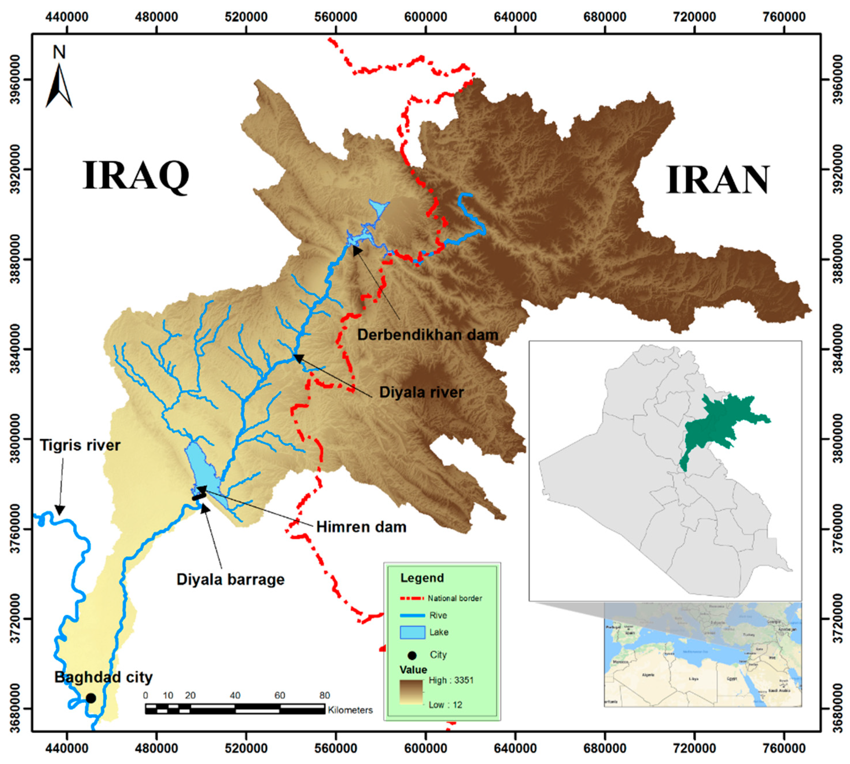
A case study in Iraq’s Diyala river basin was adopted as a real-world IWRM problem which is more complex than common benchmark test functions [22]. GWP, [71]. The Global Water Partnership defines the IWRM as “IWRM is a process which promotes the co-ordinated development and management of water, land and related resources, in order to maximize the resultant economic and social welfare in an equitable manner without compromising the sustainability of vital ecosystems”. Authors and institutes adopt different water management concepts (about 41 variant possible explanations for the term “integrated”) due to the generalization in IWRM definition. Some examples are: water supply and water demands; surface water and groundwater; water quantity and water quality; urban and rural water issues; government and NGOs (non-governmental organizations) [72,73]. The river basin has two multipurpose dams, Derbendikhan just at the northern international border in Sulaymaniya governorate, and Himren in the middle part of the basin in the Diyala governorate (Figure 3). Here, Derbendikhan dam’s operation strategy for the next three decades was selected as a benchmark problem. Based on monthly dataset from 1981 to 2012 (33 years), a total of 396 decision variables (reservoir releases) need to be managed during the time-scale. Generating hydropower is the main current operation target, hence power penstocks (tunnels) are the main reservoir outlet of the proposed management model.

2.4.1. Objectives Functions Formulae

The reservoir water budget is governing by the water balance equation, as:

$$S_{t+1}^D=S_t^D+I_t^D-R_t^D-E_t^D+P_t^D-S{E}_t^D+G{R}_t^D, t=1, 2,\dots T$$

(7)

where $S_t^D$ and $S_{t+1}^D$ are the reservoir storage at time t and t+1, $I_t^D$ and $R_t^D$ are reservoir inflows and releases, respectively. $E_t^D$ is the evaporation losses from reservoir surface, $P_t^D$ is the direct rainfall on the reservoir. While, $S{E}_t^D$ and $G{R}_t^D$ are seepage losses and groundwater recharges from the reservoir, respectively.

The reservoir operation strategy (${\mathit{F}}_D$) is represented by the following multi-objective (or many for more than 3 objectives) formula:

$$min {\mathit{F}}_D=(f_{winterD}, f_{summerD}, f_{powerD},f_{Del-SW},f_{regD})$$

(8)

where $f_{winterD}$ is for maximizing winter storage to fulfil summer demands, $f_{summerD}$ is for minimizing summer storage to absorb expected flood wave in the next season, $f_{powerD}$ is for maximizing hydropower generation, $f_{Del-SW}$ is for minimizing agriculture projects’ water deficit, and $f_{regD}$ is for minimization releases fluctuation. These targets represent the following aspects: social ($f_{winterD}$ and $f_{summerD}$); economic ($f_{powerD}$, $f_{Del-SW}$); and environmental ($f_{regD}$).

The details of these objectives functions are as follows:

$$\mathit{min}{f}_{winterD}={\displaystyle \sum }_{t=1}^{Tw}{\left(\frac{S_{max}^D-S_t^D}{S_{max}^D}\right)}^2 +C_P , t =1, 2,\mathrm{..} TW$$

(9)

$$\mathit{min}{f}_{summerD}={\displaystyle \sum }_{t=1}^{Ts}{\left(\frac{S_t^D-S_{minp}^D}{S_{max}^D}\right)}^2+C_P , t =1, 2, \mathrm{..} TS$$

(10)

$$\mathit{min}{f}_{powerD}={\displaystyle \sum }_{t=1}^T{\left(\frac{P{w}_{max}^D-P{w}_t^D}{P{w}_{max}^D}\right)}^2+C_P , t =1, 2,\mathrm{..}T$$

(11)

$$\mathit{min}{f}_{Del-SW}={\displaystyle \sum }_{t=1}^T{\left(\frac{P{D}_t-De{l}_t^M}{P{D}_{max}}\right)}^2+C_P , t =1, 2,\mathrm{..}T$$

(12)

$$\mathit{min}{f}_{regD}={\displaystyle \sum }_{t=1}^{T-1}{\left(\frac{R_t^D-R_{t+1}^D}{R_{max}^D}\right)}^2+C_P , t =1, 2,\mathrm{..}T$$

(13)

$$C_P=A\times {\displaystyle \sum }_{i=1}^{NC}{g}_i; A\ge 1 , i =1, 2, . . NC$$

(14)

Where:

$S_{max}^D$ = maximum allowable reservoir storage

$S_{minp}^D$= minimum allowable reservoir storage for hydropower generation

T_W, T_S and T = winter, summer and total operation periods, respectively.

$P{w}_t^D$= hydropower generation at time t

$P{w}_{max}^D$= maximum hydropower generation

$P{D}_t$ = projects’ water demands at time t

$P{D}_{max}$ = maximum projects’ water demands

$De{l}_t^M$ = delivered water at time t

$R_{max}^D$ = maximum reservoir releases at time t

C_P = penalty factor includes all the violations of the model, which could be expressed

NC = number of constraints

$g_i$ = penalty function for the (i^th) constraint

A = a positive real number

The hydropower generation can be expressed as:

$$P{w}_t^D={\eta }_e^D.{\gamma }_w.Q_t^{tuD}.H_t^{nD}$$

(15)

where ($Q_t^{tuD}$) is the turbine discharge, ($H_t^{nD}$) is the net head between reservoir level and the tail water after the power plant, (${\eta }_e^D$) is the efficiency of power plant, and (${\gamma }_w$) is the water density.

2.4.2. Reservoir System Constraints

The reservoir storage is limited between the minimum and maximum allowable storage,$283.48\le S_t^D\le 2572.0$ (million cubic meters), the water level head ($H_t^D$) should be $\ge 434.0$ m.a.s.l, the power generation must be less than $249000$ Kw and greater than 16000 Kw, and the release between $51.84\le R_t^D\le 878.6$ million cubic meters/month. Hence, the penalty functions ($g_i$) can be expressed as:

$$g_1={\displaystyle \sum }_{t=1}^{T}Max\left[0, \left(S_t^D-283.48\right)\right]$$

(16)

$$g_2={\displaystyle \sum }_{t=1}^{T}Max\left[0, \left(2572.0-S_t^D\right)\right]$$

(17)

$$g_3={\displaystyle \sum }_{t=1}^{T}Max\left[0, \left(H_t^D-434.0\right)\right]$$

(18)

$$g_4={\displaystyle \sum }_{t=1}^{T}Max\left[0, \left(P{w}_t^D-16000\right)\right]$$

(19)

$$g_5={\displaystyle \sum }_{t=1}^{T}Max\left[0, \left(249000-P{w}_t^D\right)\right]$$

(20)

$$g_6={\displaystyle \sum }_{t=1}^{T}Max\left[0, \left(R_t^D-51.84\right)\right]$$

(21)

$$g_7={\displaystyle \sum }_{t=1}^{T}Max\left[0, \left(878.6-R_t^D\right)\right]$$

(22)

2.5. Computational Properties

The computational parameters of the problems were 2.0 × 10⁶ function evaluations and ε = 0.1 for three objectives, and ε = 0.5 for five objectives, with 10 and 20 runs for both algorithms. The minimum population size was 100 while the maximum was 1000. A Dell OptiPlex 780 computer was used (Core Duo 2 E8400, 2 × 3.0 GHz, 8.0 GB RAM, Ubuntu 16.04 operating system).

Table 2. Parameter values used in the optimization algorithms.

Parameters	Borg	ε-DSEAa	Parameters	Borg	ε-DSEA
Initial population size	100	100	SPX parents	10	3
Tournament selection size	2	2	SPX offspring	2	2
SBX crossover rate	1.0	1.0	SPX expansion rate λ	3	[2.5, 3.5]
SBX distribution index η	15.0	[0, 100]	UNDX parents	10	10
DE crossover rate CR	0.1	[0.1, 1.0]	UNDX offspring	2	2
DE step size F	0.5	[0.5, 1.0]	UNDX σζ	0.5	[0.4, 0.6]
PCX parents	10	10	UNDX ση	0.35/$\sqrt{L}$	[0.1, 0.35]/$\sqrt{L}$
PCX offspring	2	2	UM mutation rate	1/L	1/L
PCX ση	0.1	[0.1, 0.3]	PM mutation rate	1/L	1/L
PCX σζ	0.1	[0.1, 0.3]	PM distribution index ηm	20	20

L is the number of decision variables. The permissible range for dynamic parameters is shown in brackets. The parameters σ_η and σ_ζ are defined in Table 1. ^a The initial values of dynamic parameters used in ε-DSEA are as shown for Borg MOEA.

shows the parameter values used for both algorithms. A program (code) in C language was developed to build the current model.

3. Results

3.1. Performance Achievement

3.1.1. Algorithms’ Reliability

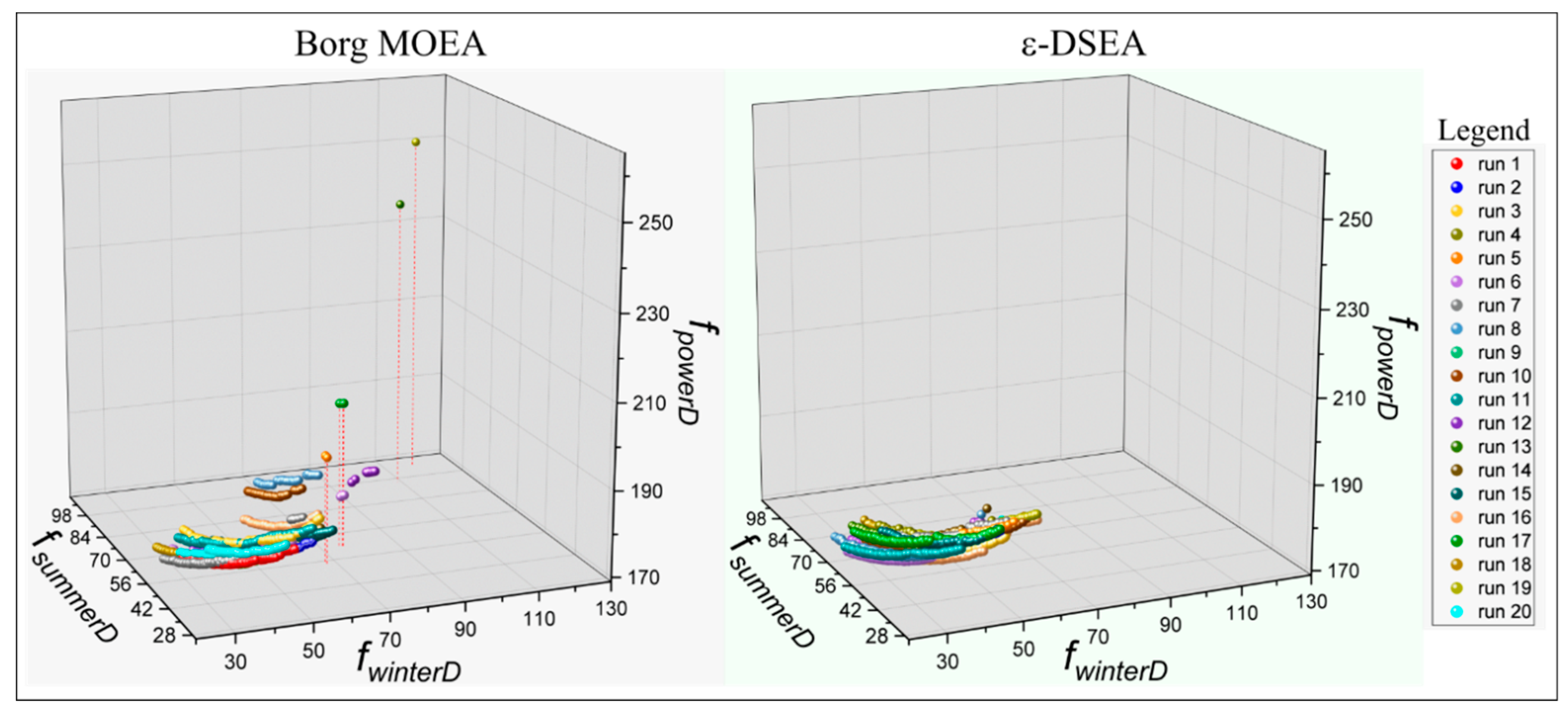
Figure 4 illustrates the Pareto-front for 20 replicated random runs of the case study benchmark problem for both algorithms using three objectives. Although both algorithms converged to possible optima, ε-DSEA shows better reliability. Notably, Borg MOEA has faced some challenges in six trials, as it was stagnant in four and had overdue convergence in two. Some of these contain only one solution, as highlighted with dotted lines. In addition, some others have discontinuous Pareto-front (with gaps) in the objective search space. This behaviour reduces an algorithm’s reliability to produce near optimal solutions over replicated random execution (for example when testing the confidence of the model output), and is a key factor when solving more complex problem using high-performance computer resources (e.g., parallel processing with multi-core). Conversely, ε-DSEA shows reliability over 20 runs to converge to the possible optimal solution, with commonly continuous Pareto-front. Hence, less randomness creeps into runs increasing the confidence that optimal solutions can be achieved.

A high-dimension problem (5 objectives) was employed for advance algorithms’ assessment as shown in Figure 5. The optimum solutions’ median for 10 trials of both algorithms is presented. Notably, both algorithms produce possible optimum solutions, but the ε-DSEA has slightly more reliable trends over execution repetitions as supported by the self-adaptive parameters’ technique used in this EA, which was also approved by [74] for 20 runs. Insight investigation shows that a Borg MOEA stack in local optima twice (run 3 and 7), and adapt with PCX operator for all trials, as in three objectives scenario; while ε-DSEA adapts at the initial stage with SBX operator, then with PCX and SPX operators in parallel for the rest of evaluation process (Figure S1 in the supplementary data). The resetting technique’s effectiveness is obvious over changing the trend of the operators’ adaptation to escape from a local optima pitfall. Execution trial No. 4 shows competitive achievement of both algorithm, which may consider for comparative investigation.

Hence, the proposed mechanism provides advance diversity and balancing between exploration and exploitation process toward possible Pareto-front set.

3.1.2. Algorithms’ Robustness and Efficiency

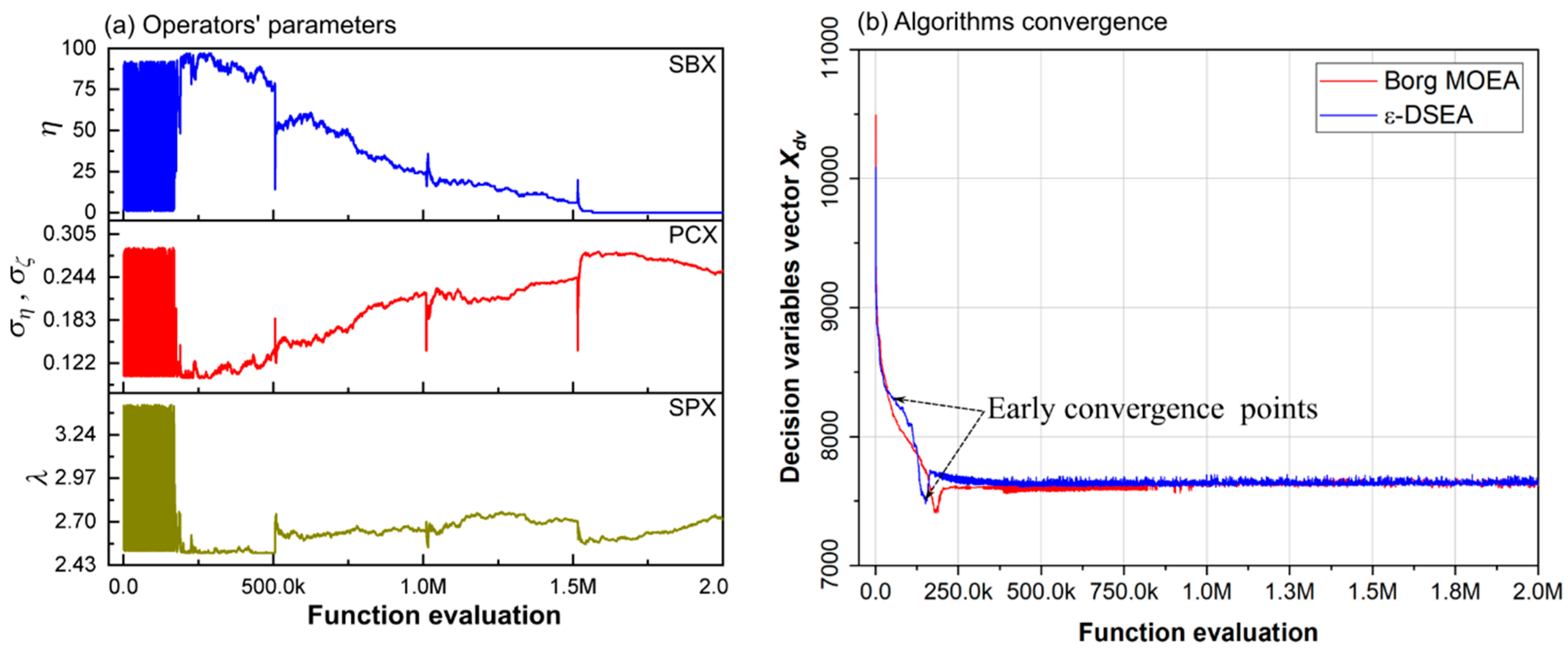
In ε-DSEA, non-dominated feedback loops control the operators’ adaptation and their parameters. Figure 6a illustrates the self-adaptive operators’ parameter-tuning behaviour of ε-DSEA during the evaluation process. The most effective operators adopted to generate dominance solutions for the best trial are SBX, PCX, and SPX. Initially the virtual dominance archive mechanism tuned the operator’s parameters when only one solution is kept in the dominance archive. Then the SBX operator was adopted until the first resetting trigger at 5.0 × 10⁵ function evaluation. The PCX operator is then involved by increasing the variation parameters (${\sigma }_{\eta }$ and ${\sigma }_{\zeta }$) to about 0.15. The SPX operator is also involved at the same time when its parameter (λ) changed to about 2.7. Both PCX and SPX operators compete to explore dominance solutions till the third resetting trigger, and after that the SPX operator starts to generate more dominance solutions in the dominance archive. Increasing PCX and SPX parameters will generate new offspring farther away from their original parents, which will increase algorithm exploration in the design search space.

The algorithms’ convergence (efficiency) also investigated using the decision variables vector ($X_{dv}$) development in the dominance archive during the evaluation process. The $X_{dv}$ is equal to $\sqrt{x_1^2+x_2^2+x_3^2+\dots +x_n^2}$ , where x₁ to x_n are the decision variables. Based on the best solution achieved, Figure 6b shows $X_{dv}$ convergence of both algorithms. Both achieved early convergence, but ε-DSEA converged faster, hence ε-DSEA’s efficiency was endorsed in the proposed test problem.

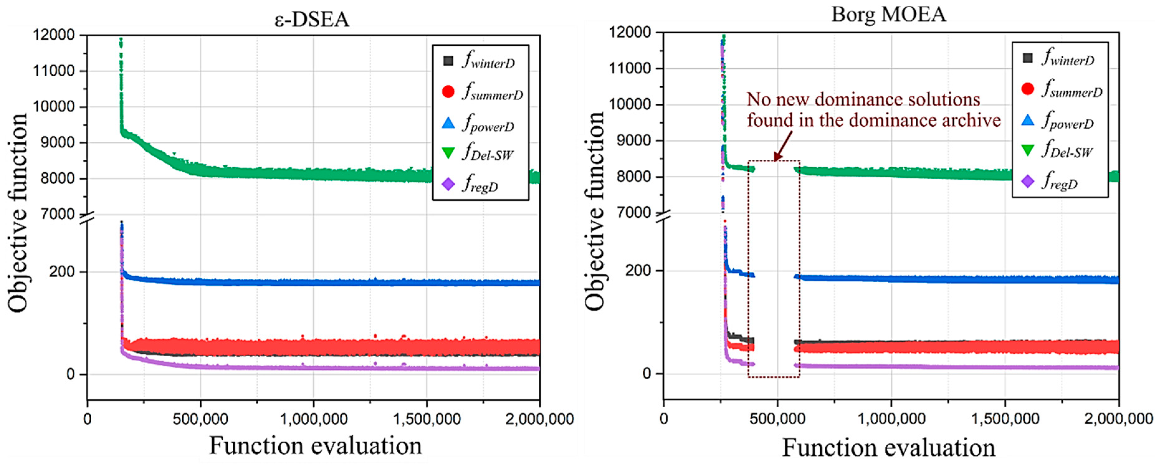
The progress of the objectives’ convergence of both algorithms over 10 iterations of high-dimension problem is presented in Figures S2 and S3 in the supplementary data, respectively. Early convergence was achieved by both algorithms, ε-DSEA converged at 1.25 × 10⁴ function evaluations for all iterations, and Borg MOEA converged at 25 × 10⁴. The ε-DSEA needs less execution time to achieve solutions. Where there are limited computational resources (e.g., CPU, Ram, etc.,) this achievement is significant. Furthermore, Borg MOEA suffered significant and interim stagnation in 7 trials (2, 3, 7, 9, and 4, 6, 10, respectively) in the early stage of evaluations. Only three out of 10 trials maintained dominance solutions improvement over the entire evaluation. The PCX operator’s adaptation with fixed parameters and recycling repetitively archive’s dominance solutions may restrict the extent of the algorithm’s exploration in the design search space. Conversely, only one trial (no. 9) suffered significate stagnation in ε-DSEA, however the expansion diversity and resetting techniques succeed in reviving the algorithm’s exploration to find new dominance solutions in the dominance archive. The robustness of ε-DSEA to escape from local optima are evident. Figure 7 shows trial no. 4 as a sample of convergence progress, since both algorithms achieved competitive solutions (based on Figure 5).

3.1.3. Algorithms’ Effectiveness

For real-world multi-objective problems, and especially in water resources management problems, the true Pareto-front (e.g., optimum solution) is unknown [22], and it is difficult to measure an algorithm’s effectiveness for such problems, as other relevant factors should also be evaluated such as the coverage of the Pareto-front and its extent in the objective space [34]. Hence, the qualitative comparison was often based on the best solution achieved over several replicated trials (e.g., equal or more than 20 runs). The results here show the reliability of both EA models but better computational performance by ε-DSEA.

3.2. Strategic Achievement

Table 3. Results’ analysis of water resources management strategy of Derbendikhan dam achieved by both algorithms based on maximising hydropower generation.

	Borg MOEA					ε-DSEA
	Area 1	Head 2	Power 3	Storage 4	Releases 5	Area	Head	Power	Storage	Releases
3 Objective problem
Min.	19.18	437.79	24.50	433.55	129.94	17.32	434.73	24.83	373.82	129.75
Max.	122.79	485.97	249.00	2565.84	866.25	121.80	485.86	246.37	2551.05	877.20
Mean	74.37	474.71	94.76	1732.33	336.06	76.39	475.53	94.77	1775.22	336.17
Median	72.03	477.12	83.00	1743.17	297.19	78.92	478.95	84.37	1867.41	316.10
St.7	27.19	10.11	50.88	523.86	174.84	24.99	10.42	51.88	496.30	183.22
Gross6			37.52	686.00	133.08			37.53	702.99	133.12
	5 Objective problem
Min.	16.94	434.09	23.44	361.60	130.72	19.10	437.67	24.09	431.16	130.45
Max.	122.97	485.98	249.00	2568.50	866.08	123.14	486.00	249.00	2570.98	797.97
Mean	66.09	470.67	90.46	1555.39	337.72	71.90	472.95	91.77	1672.36	334.80
Median	61.55	473.63	82.14	1540.19	316.81	71.78	477.05	82.00	1738.53	298.79
St.	29.89	12.83	45.64	597.36	162.74	28.94	12.58	47.18	583.53	169.11
Gross			35.82	615.94	133.74			36.34	662.25	132.58

¹ Surface area of reservoir in km²; ² Head of water in m.a.s.l; ³ Hydropower generation in MW; ⁴ Reservoir storage in m³ ×10⁶); ⁵ Reservoir releases in m³/month ×10⁶; ⁶ Gross sum units of: Power in GW; Storage in m³ ×10⁹); Releases in m³/month ×10⁹. ⁷ St. for Standard Deviation.

demonstrates results’ analysis of both algorithms’ achievement based on best optimum solution to maximise hydropower generation, as it is one of the main dam’s operation targets. The gross sum of hydropower, storage, and releases of the reservoir were presented to demonstrate the contrast between two algorithms’ achievement, based on the relevant optimization techniques. The results of both are harmonic, with advance merit of ε-DSEA.

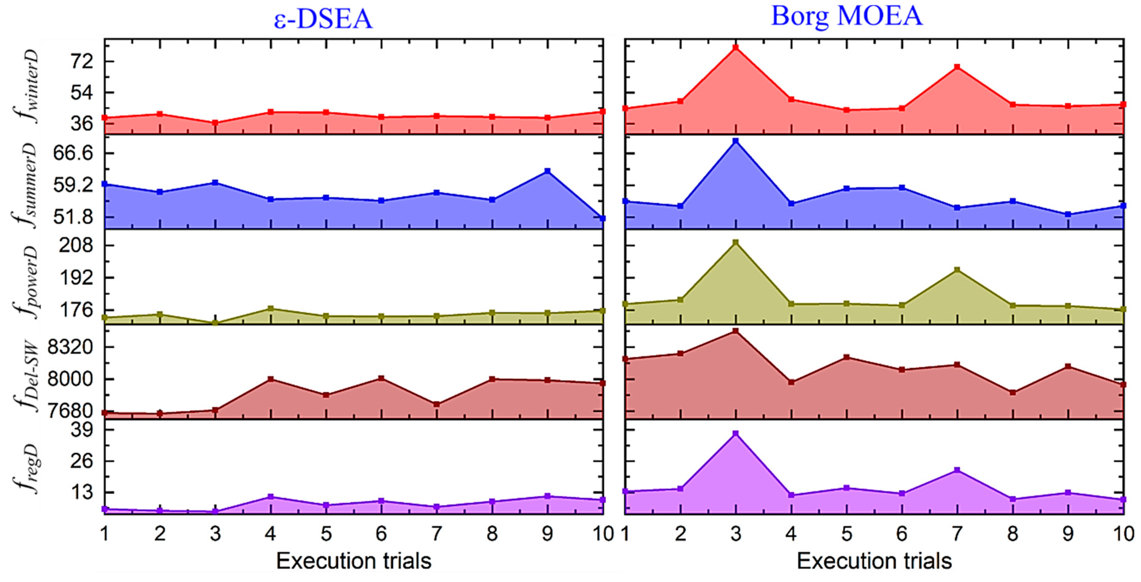
Figure 8a,b depict algorithms’ attainment of 10 multi-objective multi-variable trials and show the consistency of the ε-DSEA is marginally better than Borg notably from the period 1 to 216 months. The same behaviour also achieved for the next period, which reflect ε-DSEA algorithms’ ability to generate possible competitive optimal solution with fewer replicated trials.

Consistency with the relevant historical (actual) dataset should also be reviewed during decision making trials (i.e. solutions’ quality), as in Figure 8c,d. Both algorithms achieved competitive results, but ε-DSEA’s result has better reaction to flood waves and better agreement with the historical data. Here, spillway discharge did not factor in the models or the developed management model, since flood waves events usually last hours or a couple of days in the investigated region. Accordingly, no relevant sensitive reaction was observed since monthly average management was adopted by the model.

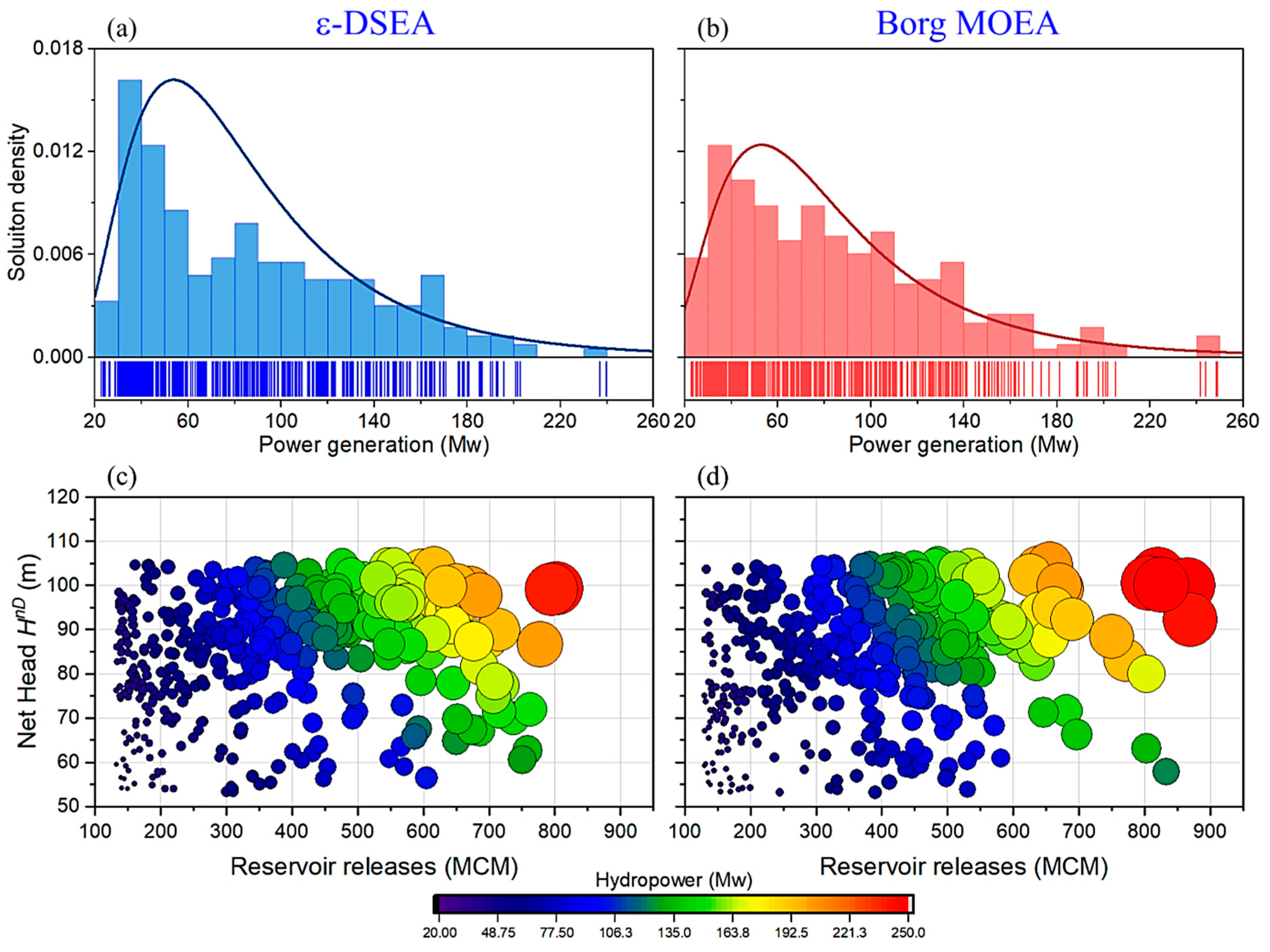
As a source of renewable energy, hydropower generation is one of the key-operational targets of the tested real-world problem, and often for any multipurpose dam projects, that needs to be carefully management under different operation scenarios, such as flood risk management. Two objectives were adopted, $f_{winterD}$ and $f_{summerD}$, the later selected for insight investigation, as it is the most critical operation scenario that may affect other operational targets. Figure 9a,b illustrate solution distribution density achieved by both algorithms over the power generation domain. In general, ε-DSEA achieved high repetition of 30 to 50 Mw solutions, and gentle gradient repetition after that, while Borg MOEA has steeper gradient repetition starting from 30 Mw and thereafter. ε-DSEA achievement offers insight for investment decision making as minimum power generation of 30 Mw could be guaranteed for next three decades.

Hydropower generation depends on two variables, turbine’s discharge and water net head, as in Equation (15) (turbine’s efficiency and water’s specific weight assumed constant). Figure 9c,d illustrate hydropower generation solution’s space achieved by both algorithms. Competitive distribution over solution space was accomplished by both algorithms for turbine discharge ≤600 MCM, while better space’s exploitation for greater values (>600 MCM) achieved by ε-DSEA. Borg tends to maximize power generation by releasing more water, but solutions are irregularly deployed (clustering) which possibly due to local optima pitfall.

For example, in the region of <80m net head ($H^{nD}$) and >600 MCM releases (Figure 9c,d), only five solutions formed as two groups achieved (green colour), which is not the case in ε-DSEA.

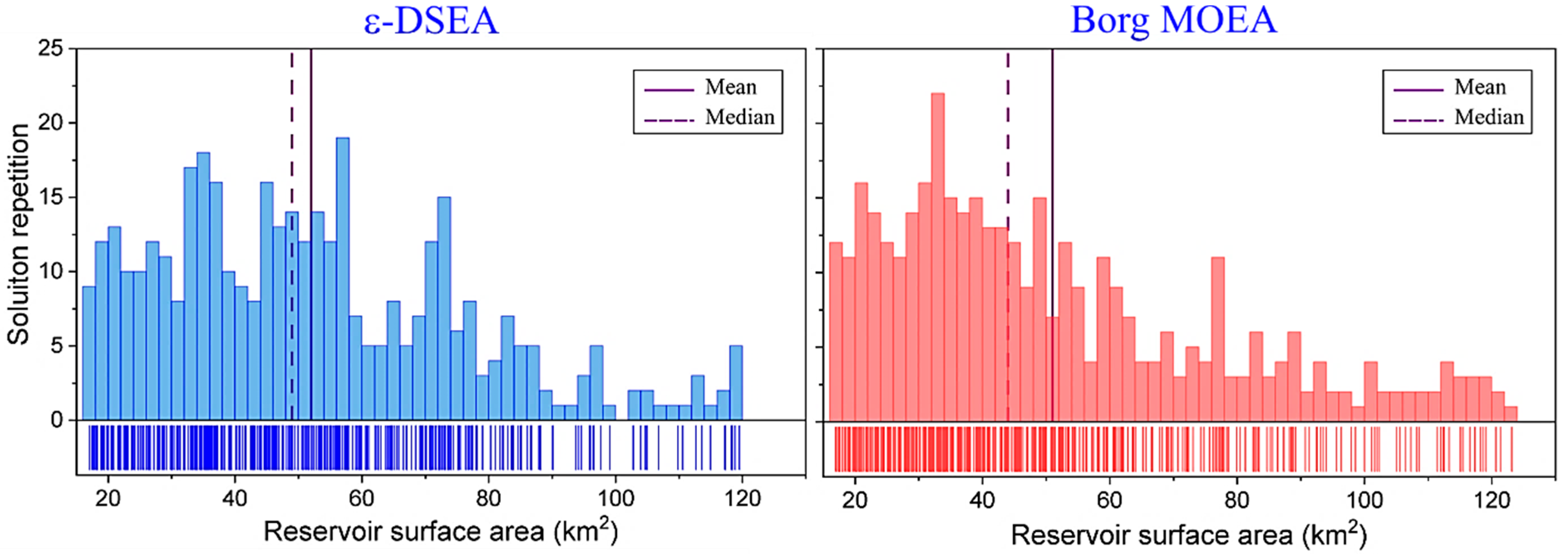
Recreation is another target to optimize for revenue. Figure 10 shows reservoir surface area achieved by both algorithms for the considered time-scale of $f_{summerD}$ scenario. The mean and median surface area were about 52 and 49 km², 51 and 44 km² achieved by ε-DSEA and Borg respectively. The small violation between these values indicates competitive results’ distribution, corollary more solutions greater than these values achieved by ε-DSEA. Hence, projects’ revenues could be improved even in such a critical scenario.

4. Discussion

4.1. Algorithms’ Optimization Techniques

The technique of Borg MOEA tends to adapt based on operator experience after finding possible feasible solutions. The SBX operator was adopted in the early stage of evaluation process, then PCX operator adopted to the end. Zheng et al., [48] observed that, for two-objective problems, Borg MOEA tended to converge prematurely and population diversity decreased relatively rapidly. This is because Borg MOEA does not maintain a separate transient sub-population of offspring as in NSGA-II. Offspring that dominate its parents immediately replaces one of the parents; the choice of the parent that is replaced is random. As new solutions are introduced, the selection pressure on less competitive solutions increases, due to the binary tournament selection used for a crossover. Fitting solutions have a higher probability of selection for a crossover, leading to more exploitation and less exploration and thus less diversity. Secondly, the injection trigger that depends mainly on ε-progress indicators, did not always succeed in reflecting stagnation during the evaluation process. Thirdly, PCX operator produces offspring in the vicinity of the parents. If the PCX operator creates solutions around the best solutions, the PCX-generated solutions quickly dominate the archive, leading to more exploitation, less exploration and consequently relatively rapid loss of diversity. As stated previously, the recombination operators are deployed in proportion to the number of offspring they contributed in the archive.

In Borg MOEA the operator that produces more successful (i.e., non-dominated) offspring is deployed more frequently. However, as the search progresses and the balance between exploration and exploitation shifts gradually, it is desirable that the operators be deployed based on the current status of the search rather than their previous performances or cumulative successes. In other words, the selection of the operators should recognize the current performance also. Hence, the proposed performance assessment of the operators relies on the results from the current phase of the search rather than the cumulative performance to date.

The novel technique of virtual dominance archive used in ε-DSEA removes operator bias and extends the algorithm’s exploration by tuning the operators’ parameters control within the specified domain, resulting in a robust convergence progress at initial stage of the evaluation process. In the same context, resetting these parameters’ values during evaluation process help the algorithm to escape from local optima pitfall, and improve its exploitation to find new non-dominated solutions.

4.2. Water Resources Management Case Study

Although both algorithms achieved possible optimum solutions, ε-DSEA generates more robust results. Based on gross sum of five objective problems (Table 3), an extra 520 MW and 46.31 MCM of hydropower generation and reservoir storage was achieved, respectively. The mean and median water head achieved by ε-DSEA were about 1.5 m higher than those of Borg MOEA in all cases. This will provide advance security against possible dam failures in the future as the water head should be above 455.0 m.a.s.l [75]. Although this problematic was not considered in the current model as an objective or a constraint, all the relevant mean and median values achieved by both algorithms satisfy this restriction. This area of study should be considered in future work.

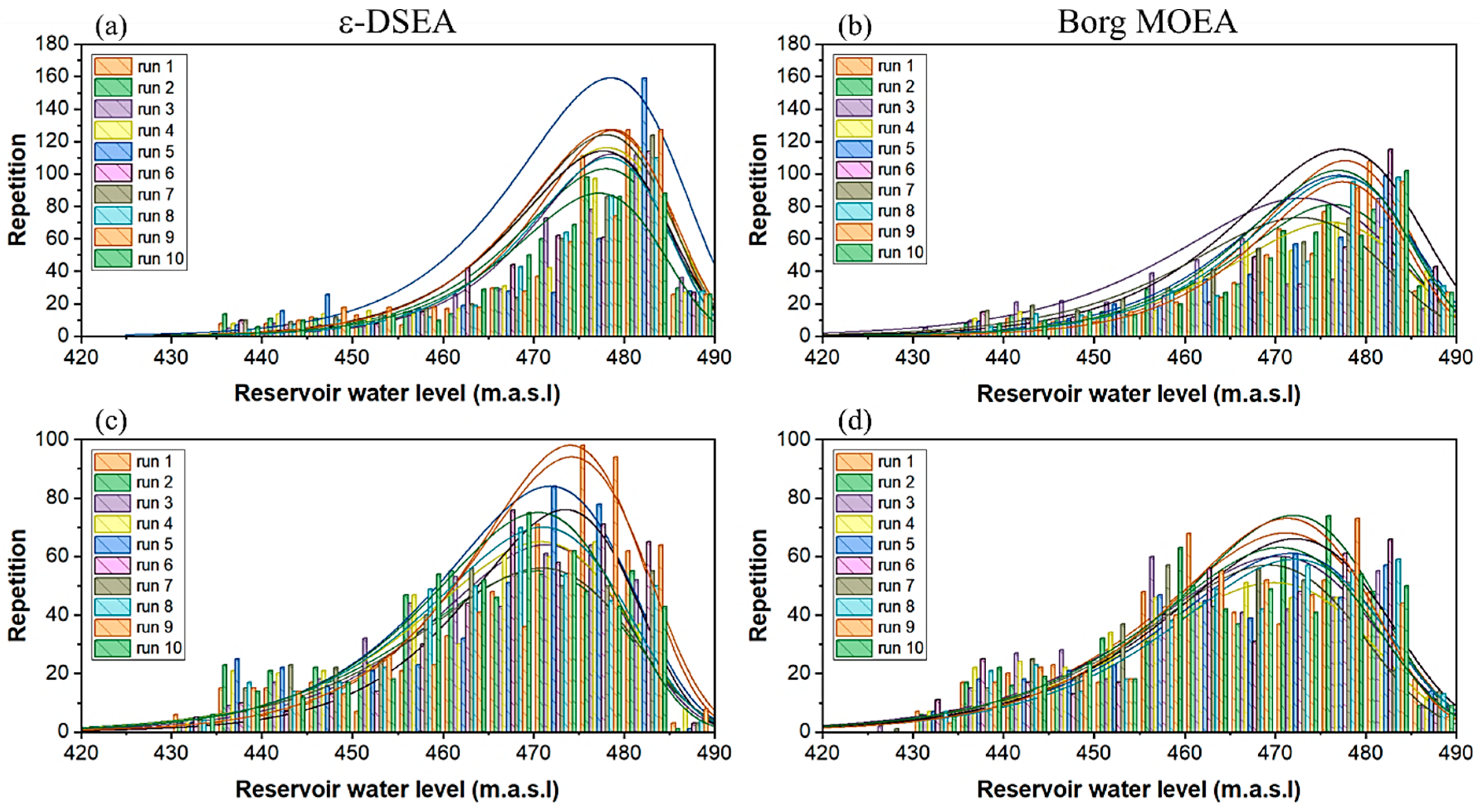
Figure 11a,b illustrates results’ quality of reservoir water level (m.a.s.l) produced by both algorithms over 10 runs, based on maximizing hydropower generation. Notably, more results of ≥460.0 and fewer of ≤440.0 were generated by ε-DSEA. The same achievement observed in the critical scenario of minimizing storage in summer, represented by $f_{summerD}$, as in Figure 11c,d. Nevertheless, the latter has better results’ than Borg MOEA regarding the current potential risk. Moreover, the harmony of results’ distribution over 10 trials is evident, endorsing the reliability of ε-DSEA.

Within this framework, good exploration-exploitation balance of slave (or secondary) solution search space of hydropower generation and reservoir surface area were attained (Figure 9). Although the master decision variables’ search space is relevant to reservoir releases while other dependent variables are calculated accordingly (e.g., power generation, storage, area, etc.), the compete optimality achievement mapped to those sub-variables. This is not the case in other optimization algorithms, since often competitive investigation only covers the master decision variables and/or objectives’ search space, either in test functions or in real-world case study benchmarks. Insight or deep diagnosis assessment considering indirect variables should be used in such competitive studies.

The results suggest water resources decision makers are advised to implement different optimization algorithms, especially when solving multi or many objective problems, to explore possible new optimal results with advance quality, and to reinforce results’ reliability. The ε-DSEA achievement was previously assessed using more complex water resources problem, as in [74,76], however, more assessment is recommended to solve different problem environments.

5. Conclusions

In this research, strategic planning of water resources under competitive optimization techniques was investigated. Decision makers often adopt optimization techniques to evaluate a wide range of competitive water resources management decisions. However, past studies demonstrate that an algorithm’s optimal output varies according to the problem environment. Furthermore, slave (dependent) variables’ quality are often not analysed in depth, which could play an important role in improving a project’s economic success. Here, a comparative assessment of two optimization techniques was tested against a real-world water resources strategy. The Borg MOEA and the ε-DSEA performance was contrasted based on the relevant strategic plans using objective functions (i.e., the Pareto-front), master and slave variables.

The results by both models showed possible optima, with an advanced reliability and robustness when using ε-DSEA as it provided consistent results closer to near-optimal solutions. Both algorithms have auto-adaptive operator techniques, but Borg appoints a mono-operator after a specific number of evaluations (e.g., PCX), while multi-operators sequence during the evaluation stages (e.g., starting by SBX operator and ending with PCX and SPX operators in parallel). The Borg MOEA reviver’s techniques should consider this drawback, as early stages stagnation is evident, especially in many-objectives problem. The ε-DSEA escapes from local optima by employing by-stage operators’ parameters, which may be useful when applying to real-world problem solving.

The compete achievement of ε-DSEA was mapped onto the relevant water resources strategic plan. In all adopted scenarios for the real-world case study results show that extra hydropower, reservoir storage and surface area can be achieved. The releases have better consistency and sensitivity with the historical dataset and flood waves. The model outputs can be used to manage power generation to support, for example, an investment opportunity while still promising recreation investment opportunities achieved by maintaining larger reservoir surface area over the adopted time-scale. The results demonstrate the importance of insight and in-depth analysis of relevant objectives and variables using EA models.

The ε-DSEA and the relevant approach could be evolve for similar and/or even more complex real-world problems, such as groundwater management, water supply system, water allocation, etc., by adding and/or modifying objective functions, decision variables, and constraints.

References

- Maier, H.; Kapelan, Z.; Kasprzyk, J.; Matott, L. Thematic issue on Evolutionary Algorithms in Water Resources. Environ. Model. Softw. 2015, 69, 222–225. [Google Scholar] [CrossRef] [Green Version]
- Holland, J.H. Adaptation in Natural and Artificial Systems: An Introductory Analysis with Applications to Biology, Control, and Artificial Intelligence; University of Michigan Press: Ann Arbor, MI, USA, 1975. [Google Scholar]
- Schaffer, J.D. Multiple objective optimization with vector evaluated genetic algorithms. In Proceedings of the 1st international Conference on Genetic Algorithms; 1985; pp. 93–100. [Google Scholar]
- Deb, K.; Pratap, A.; Agarwal, S.; Meyarivan, T. A fast and elitist multiobjective genetic algorithm: NSGA-II. IEEE Trans. Evol. Comput. 2002, 6, 182–197. [Google Scholar] [CrossRef] [Green Version]
- Zhang, Q.; Li, H. MOEA/D: A Multiobjective Evolutionary Algorithm Based on Decomposition. IEEE Trans. Evol. Comput. 2007, 11, 712–731. [Google Scholar] [CrossRef]
- Zitzler, E.; Künzli, S. Indicator-Based Selection in Multiobjective Search. Computer Vision ECCV 2012 2004, 3242, 832–842. [Google Scholar]
- Storn, R.; Price, K. Differential Evolution—A Simple and Efficient Heuristic for global Optimization over Continuous Spaces. J. Glob. Optim. 1997, 11, 341–359. [Google Scholar] [CrossRef]
- Eberhart, R.; Kennedy, J. A new optimizer using particle swarm theory. In Proceedings of the Sixth International Symposium on Micro Machine and Human Science, Nagoya, Japan, 4–6 October 1995; pp. 39–43. [Google Scholar]
- Dorigo, M.; Stützle, T. Ant Colony Optimization; Bradford Company: Scituate, MA, USA, 2004. [Google Scholar]
- Kirkpatrick, S.; Gelatt, C.D.; Vecchi, M.P. Optimization by Simulated Annealing. Science 1983, 220, 671–680. [Google Scholar] [CrossRef] [PubMed]
- Coello, C.A.C.; Lamont, G.L.; van Veldhuizen, D.A. Evolutionary Algorithms for Solving Multi-Objective Problems, 2nd ed.; Springer: Berlin/Heidelberg, Germany, 2007. [Google Scholar]
- Zhou, A.; Qu, B.-Y.; Li, H.; Zhao, S.-Z.; Suganthan, P.N.; Zhang, Q. Multiobjective evolutionary algorithms: A survey of the state of the art. Swarm Evol. Comput. 2011, 1, 32–49. [Google Scholar] [CrossRef]
- Hurford, A.P.; Huskova, I.; Harou, J.J. Using many-objective trade-off analysis to help dams promote economic development, protect the poor and enhance ecological health. Environ. Sci. Policy 2014, 38, 72–86. [Google Scholar] [CrossRef]
- Qi, Y.; Bao, L.; Ma, X.; Miao, Q.; Li, X. Self-adaptive Multi-objective Evolutionary Algorithm based on Decomposition for Large-scale problems: A Case Study on Reservoir Flood Control Operation. Inf. Sci. 2016, 367–368, 529–549. [Google Scholar] [CrossRef]
- Salazar, J.Z.; Reed, P.M.; Quinn, J.D.; Giuliani, M.; Castelletti, A. Balancing exploration, uncertainty and computational demands in many objective reservoir optimization. Adv. Water Resour. 2017, 109, 196–210. [Google Scholar] [CrossRef]
- Al-Jawad, J.Y.S.; Tanyimboh, T.T. Reservoir operation using a robust evolutionary optimization algorithm. J. Environ. Manag. 2017, 197, 275–286. [Google Scholar] [CrossRef] [PubMed] [Green Version]
- Dai, L.; Zhang, P.; Wang, Y.; Jiang, D.; Dai, H.; Mao, J.; Wang, M. Multi-objective optimization of cascade reservoirs using NSGA-II: A case study of the Three Gorges-Gezhouba cascade reservoirs in the middle Yangtze River, China. Hum. Ecol. Risk Assess. Int. J. 2017, 23, 1–22. [Google Scholar] [CrossRef]
- Hadka, D.; Reed, P. Diagnostic Assessment of Search Controls and Failure Modes in Many-Objective Evolutionary Optimization. Evol. Comput. 2012, 20, 423–452. [Google Scholar] [CrossRef] [PubMed]
- Li, K.; Deb, K.; Zhang, Q.; Kwong, S. An Evolutionary Many-Objective Optimization Algorithm Based on Dominance and Decomposition. IEEE Trans. Evol. Comput. 2015, 19, 694–716. [Google Scholar] [CrossRef]
- Liu, Z.-Z.; Wang, Y.; Huang, P.-Q. AnD: A many-objective evolutionary algorithm with angle-based selection and shift-based density estimation. Inf. Sci. 2018, 1–20. [Google Scholar] [CrossRef]
- Ishibuchi, H.; Setoguchi, Y.; Masuda, H.; Nojima, Y. Performance of Decomposition-Based Many-Objective Algorithms Strongly Depends on Pareto Front Shapes. IEEE Trans. Evol. Comput. 2017, 21, 1. [Google Scholar] [CrossRef]
- Maier, H.; Kapelan, Z.; Kasprzyk, J.; Kollat, J.; Matott, L.; Cunha, M.; Dandy, G.; Gibbs, M.; Keedwell, E.; Marchi, A.; et al. Evolutionary algorithms and other metaheuristics in water resources: Current status, research challenges and future directions. Environ. Model. Softw. 2014, 62, 271–299. [Google Scholar] [CrossRef] [Green Version]
- Goldberg, D.E. Sizing Populations for Serial and Parallel Genetic Algorithms. In Proceedings of the 3rd International Conference on Genetic Algorithms, San Francisco, CA, USA, 4–7 June 1989; pp. 70–79. [Google Scholar]
- De Jong, K. Parameter Setting in EAs: A 30 Year Perspective. Informatik im Fokus 2007, 54, 1–18. [Google Scholar]
- Karafotias, G.; Hoogendoorn, M.; Eiben, A.E. Parameter Control in Evolutionary Algorithms: Trends and Challenges. IEEE Trans. Evol. Comput. 2015, 19, 167–187. [Google Scholar] [CrossRef]
- Eiben, A.; Hinterding, R.; Michalewicz, Z. Parameter control in evolutionary algorithms. IEEE Trans. Evol. Comput. 1999, 3, 124–141. [Google Scholar] [CrossRef]
- Deb, K.; Agrawal, R.B. Simulated Binary Crossover for Continuous Search Space. Complex Syst. 1995, 9, 115–148. [Google Scholar]
- Reynoso-Meza, G.; Sanchis, J.; Blasco, X.; Mart´ınez, M. An empirical study on parameter selection for multiobjective optimization algorithms using Differential Evolution. In Proceedings of the 2011 IEEE Symposium on Differential Evolution (SDE), Paris, France, 11–15 April 2011; pp. 1–7. [Google Scholar]
- Stephens, C.R.; Olmedo, I.G.; Mora-Vargas, J.; Waelbroeck, H. Self-Adaptation in Evolving Systems. Artif. Life 1998, 4, 183–201. [Google Scholar] [CrossRef] [PubMed]
- Hadka, D.; Reed, P. Borg: An Auto-Adaptive Many-Objective Evolutionary Computing Framework. Evol. Comput. 2013, 21, 231–259. [Google Scholar] [CrossRef] [PubMed]
- Reed, P.; Hadka, D.; Herman, J.; Kasprzyk, J.; Kollat, J.; Reed, P.; Herman, J.; Kasprzyk, J. Evolutionary multiobjective optimization in water resources: The past, present, and future. Adv. Water Resour. 2013, 51, 438–456. [Google Scholar] [CrossRef]
- Marchi, A.; Dandy, G.; Wilkins, A.; Rohrlach, H. Methodology for Comparing Evolutionary Algorithms for Optimization of Water Distribution Systems. J. Water Resour. Plan. Manag. 2014, 140, 22–31. [Google Scholar] [CrossRef]
- Silver, E.A. An overview of heuristic solution methods. J. Oper. Res. Soc. 2004, 55, 936–956. [Google Scholar] [CrossRef]
- Zitzler, E.; Deb, K.; Thiele, L. Comparison of Multiobjective Evolutionary Algorithms: Empirical Results. Evol. Comput. 2000, 8, 173–195. [Google Scholar] [CrossRef] [PubMed] [Green Version]
- Deb, K. Multi-Objective Optimization using Evolutionary Algorithms, 1st ed.; John Wiley & Sons: Chichester, UK, 2001. [Google Scholar]
- Stadler, W. A survey of multicriteria optimization or the vector maximum problem, part I: 1776–1960. J. Optim. Theory Appl. 1979, 29, 1–52. [Google Scholar] [CrossRef]
- Miettinen, K. Nonlinear Multiobjective Optimization; Kluwer Academic Publishers: Boston, MA, USA, 1999. [Google Scholar]
- Deb, K.; Joshi, D.; Anand, A. Real-coded evolutionary algorithms with parent-centric recombination. In Proceedings of the 2002 Congress on Evolutionary Computation, Honolulu, HI, USA, 12–17 May 2002; Volume 1, pp. 61–66. [Google Scholar]
- Kita, H.; Ono, I.; Kobayashi, S. Multi-parental extension of the unimodal normal distribution crossover for real-coded genetic algorithms. In Proceedings of the 1999 Congress on Evolutionary Computation-CEC99, Washington, DC, USA, 6–9 July 1999; pp. 1581–1587. [Google Scholar]
- Tsutsui, S.; Yamamura, M.; Higuchi, T. Multi-parent recombination with simplex crossover in real coded genetic algorithms. In Proceedings of the 1999 Genetic and Evolutionary Computation Conference, San Francisco, CA, USA, 13–17 July 1999; pp. 657–664. [Google Scholar]
- Michalewicz, Z.; Logan, T.; Swaminathan, S. Evolutionary operators for continuous convex parameter spaces. In Proceedings of the 3rd Annual Conference on Evolutionary Programming; 1994; pp. 84–97. [Google Scholar]
- Deb, K.; Agrawal, S. A Niched-Penalty Approach for Constraint Handling in Genetic Algorithms. Artif. Neural Nets Genet. Algorithms 1999, 4, 235–243. [Google Scholar]
- Geetha, T.; Mahalakshmi, K.; UmmuSalma, I.; Kumaran, K.M. An Observational Analysis of Genetic Operators. Int. J. Comput. Appl. 2013, 63, 24–34. [Google Scholar] [CrossRef]
- Laumanns, M.; Thiele, L.; Deb, K.; Zitzler, E. Combining Convergence and Diversity in Evolutionary Multiobjective Optimization. Evol. Comput. 2002, 10, 263–282. [Google Scholar] [CrossRef] [PubMed]
- Deb, K.; Manikanth, M.; Shikhar, M. A Fast Multi-Objective Evolutionary Algorithm for Finding Well-Spread Pareto-Optimal Solutions; KanGAL Technical Report No.2003002; IIT: Kanpur, India, 2003. [Google Scholar]
- Kollat, J.; Reed, P. A computational scaling analysis of multiobjective evolutionary algorithms in long-term groundwater monitoring applications. Adv. Water Resour. 2007, 30, 408–419. [Google Scholar] [CrossRef]
- Zecchin, A.C.; Simpson, A.R.; Maier, H.R.; Marchi, A.; Nixon, J.B.; Maier, H. Improved understanding of the searching behavior of ant colony optimization algorithms applied to the water distribution design problem. Water Resour. Res. 2012, 48. [Google Scholar] [CrossRef] [Green Version]
- Zheng, F.; Simpson, A.R.; Zecchin, A.C.; Maier, H.R.; Feifei, Z. Comparison of the Searching Behavior of NSGA-II, SAMODE, and Borg MOEAs Applied to Water Distribution System Design Problems. J. Water Resour. Plan. Manag. 2016, 142. [Google Scholar] [CrossRef]
- Vrugt, J.A.; Robinson, B.A. Improved evolutionary optimization from genetically adaptive multimethod search. Proc. Natl. Acad. Sci. USA 2007, 104, 708–711. [Google Scholar] [CrossRef] [Green Version]
- Hesser, J.; Männer, R. Towards an optimal mutation probability for genetic algorithms. In Parallel Problem Solving from Nature, Proceedings of 1st Workshop PPSN I Dortmund, FRG, 1–3 October 1990; Schwefel, H.-P., Männer, R., Eds.; Springer: Berlin/Heidelberg, Germany, 1991; pp. 23–32. [Google Scholar]
- Aleti, A. An Adaptive Approach to Controlling Parameters of Evolutionary Algorithms. PhD. Thesis, Swinburne University of Technology, Melbourne, Australia, 2012. [Google Scholar]
- Deb, K.; Beyer, H.-G. Self-Adaptive Genetic Algorithms with Simulated Binary Crossover. Evol. Comput. 2001, 9, 197–221. [Google Scholar] [CrossRef] [PubMed]
- Farmani, R.; Wright, J.A. Self-adaptive fitness formulation for constrained optimization. IEEE Trans. Evol. Comput. 2003, 7, 445–455. [Google Scholar] [CrossRef] [Green Version]
- Giger, M.; Keller, D.; Ermanni, P. AORCEA—An adaptive operator rate controlled evolutionary algorithm. Comput. Struct. 2007, 85, 1547–1561. [Google Scholar] [CrossRef]
- Kaveh, A.; Shahrouzi, M. Dynamic selective pressure using hybrid evolutionary and ant system strategies for structural optimization. Int. J. Numer. Methods Eng. 2008, 73, 544–563. [Google Scholar] [CrossRef]
- Vafaee, F.; Nelson, P.C. An explorative and exploitative mutation scheme. In Proceedings of the IEEE Congress on Evolutionary Computation, Barcelona, Spain, 18–23 July 2010; pp. 1–8. [Google Scholar]
- Vrugt, J.A.; Robinson, B.A.; Hyman, J.M. Self-adaptive multimethod search for global optimization in real-parameter spaces. IEEE Trans. Evol. Comput. 2009, 13, 243–259. [Google Scholar] [CrossRef]
- Lwin, K.; Qu, R.; Kendall, G. A learning-guided multi-objective evolutionary algorithm for constrained portfolio optimization. Appl. Soft Comput. 2014, 24, 757–772. [Google Scholar] [CrossRef]
- Bechikh, S.; Datta, R.; Gupta, A. Recent Advances in Evolutionary Multi-objective Optimization, Adaptation, Learning, and Optimization; Springer International Publishing: Cham, Switzerland, 2017; Volume 20. [Google Scholar]
- Li, B.; Li, J.; Tang, K.; Yao, X. Many-Objective Evolutionary Algorithms: A Survey. ACM Comput. Surv. 2015, 48, 13:1–13:35. [Google Scholar] [CrossRef]
- Mane, S.U.; Rao, M.R.N. Many-Objective Optimization: Problems and Evolutionary Algorithms—A Short Review. Int. J. Appl. Eng. Res. 2017, 12, 973–4562. [Google Scholar]
- Bechikh, S.; Elarbi, M.; Said, L.B. Many-objective Optimization Using Evolutionary Algorithms: A Survey. In Recent Advances in Evolutionary Multi-objective Optimization; Bechikh, S., Datta, R., Gupta, A., Eds.; Springer: Cham, Switzerland, 2017; pp. 105–137. [Google Scholar]
- Kollat, J.; Reed, P. Comparing state-of-the-art evolutionary multi-objective algorithms for long-term groundwater monitoring design. Adv. Water Resour. 2006, 29, 792–807. [Google Scholar] [CrossRef]
- Goldberg, D.E. Genetic Algorithms in Search, Optimization and Machine Learning, 1st ed.; Addison-Wesley Longman Publishing Co., Inc.: Boston, MA, USA, 1989. [Google Scholar]
- Zitzler, E. Evolutionary Algorithms for Multiobjective Optimization: Methods and Applications. Ph.D. Thesis, Swiss Federal Institute of Technology, Zurich, Switzerland, 1999. [Google Scholar]
- Van Veldhuizen, D.A.; Lamont, G.B. Evolutionary Computation and Convergence to a Pareto Front. In Proceedings of the Late Breaking Papers at the Genetic Programming 1998 Conference, Madison, WI, USA, 22–25 July 1998; pp. 221–228. [Google Scholar]
- Hadka, D.; Reed, P.M.; Simpson, T.W. Diagnostic assessment of the borg MOEA for many-objective product family design problems. In Proceedings of the 2012 IEEE Congress on Evolutionary Computation, Brisbane, Australia, 10–15 June 2012; pp. 1–10. [Google Scholar]
- Woodruff, M.J.; Reed, P.M.; Simpson, T.W. Many objective visual analytics: Rethinking the design of complex engineered systems. Struct. Multidiscip. Optim. 2013, 48, 201–219. [Google Scholar] [CrossRef]
- Salazar, J.Z.; Reed, P.M.; Herman, J.D.; Giuliani, M.; Castelletti, A. A diagnostic assessment of evolutionary algorithms for multi-objective surface water reservoir control. Adv. Water Resour. 2016, 92, 172–185. [Google Scholar] [CrossRef] [Green Version]
- Yan, D.; Ludwig, F.; Huang, H.Q.; Werners, S.E. Many-objective robust decision making for water allocation under climate change. Sci. Total Environ. 2017, 607, 294–303. [Google Scholar] [CrossRef]
- GWP (Global Water Partnership). Sharing Knowledge for Equitable, Efficient and Sustainable Water Resources Management; Version 2; Global Water Partnership (GWP): Stockholm, Sweden, 2003. [Google Scholar]
- Cardwell, H.E.; Cole, R.A.; Cartwright, L.A.; Martin, L.A. Integrated Water Resources Management: Definitions and Conceptual Musings. J. Contemp. Water Res. Educ. 2006, 135, 8–18. [Google Scholar] [CrossRef]
- Biswas, A.K. Integrated Water Resources Management: Is It Working? Int. J. Water Resour. Dev. 2008, 24, 5–22. [Google Scholar] [CrossRef]
- Al-Jawad, J.Y.; Alsaffar, H.M.; Bertram, D.; Kalin, R.M. A Comprehensive Optimum Integrated Water Resources Management Approach for Multidisciplinary Water Resources Management Problems. J. Environ. Manag. 2018, in press. [Google Scholar] [CrossRef]
- World Bank. Dokan and Derbendikhan Dam Inspections Report; Consultant Services by SMEC International Pty. Ltd.: Melbourne, Australia, 2006. [Google Scholar]
- Al-Jawad, J.Y.; Alsaffar, H.M.; Bertram, D.; Kalin, R.M. Optimum socio-environmental flows approach for reservoir operation strategy using many-objectives evolutionary optimization algorithm. Sci. Total Environ. 2018, 651, 1877–1891. [Google Scholar] [CrossRef] [PubMed] [Green Version]
Figure 1.
Illustrates operator’s parents’ selection from the entire population candidates after the initial random seeding at the beginning of the evaluation process.
Figure 2.
Illustrates the self-adaptive mechanism (a) and exploration extension (b) used by ε-DSEA.
Figure 3.
Catchment area of the transboundary Diyala river basin in Iraq.
Figure 4.
Pareto-fronts for twenty random runs achieved by both algorithms.
Figure 5.
Five objectives’ median optimum solutions of 10 runs of both algorithms.
Figure 6.
(a) Parameters self-adaptation of the most effective operators for the best solution achieved, and (b) algorithm convergence to generate dominance solutions during the evaluation process.
Figure 7.
Convergence progress during evaluation process of both algorithms for trial no. 4.
Figure 8.
Comparative graphs between achieved releases of both algorithms based on maximizing hydropower generation objective. (a) and (b) show detail results for 10 runs, while (c) and (d) illustrate historical and model releases.
Figure 9.
Insight analysis of hydropower generation accomplished by both algorithms under flood risk management scenario (). (a) and (b) shows solutions repetition density, while (c) and (d) demonstrate head-discharge-hydropower solution space.
Figure 10.
Reservoir’s surface area distribution achieved by both algorithms under scenario.
Figure 11.
Demonstrates reservoir water level distribution achieved by both algorithms of 10 runs. (a) and (b) are the best solution to maximize hydropower generation; (c) and (d) the same as those to minimize summer storage.