Assessment of Rainfall Kinetic-Energy–Intensity Relationships
by
 , ,
, ,
Claudio Mineo
1,* ,
,
Elena Ridolfi
2,3,
Benedetta Moccia
1,
Fabio Russo
1 and 
Francesco Napolitano
1 1
DICEA, Dipartimento di Ingegneria Civile, Edile e Ambientale, Università degli Studi di Roma, La Sapienza, 00184 Rome, Italy
2
Department of Earth Sciences, Uppsala University, 75236 Uppsala, Sweden
3
Centre of Natural Hazards and Disaster Science, CNDS, 75236 Uppsala, Sweden
*
Author to whom correspondence should be addressed.
Water 2019, 11(10), 1994; https://doi.org/10.3390/w11101994
Submission received: 1 September 2019
/
Revised: 19 September 2019
/
Accepted: 21 September 2019
/
Published: 25 September 2019
(This article belongs to the Section Hydrology)
Abstract
:Raindrop-impact-induced erosion starts when detachment of soil particles from the surface results from an expenditure of raindrop energy. Hence, rain kinetic energy is a widely used indicator of the potential ability of rain to detach soil. Although it is widely recognized that knowledge of rain kinetic energy plays a fundamental role in soil erosion studies, its direct evaluation is not straightforward. Commonly, this issue is overcome through indirect estimation using another widely measured hydrological variable, namely, rainfall intensity. However, it has been challenging to establish the best expression to relate kinetic energy to rainfall intensity. In this study, first, kinetic energy values were determined from measurements of an optical disdrometer. Measured kinetic energy values were then used to assess the applicability of the rainfall intensity relationship proposed for central Italy and those used in the major equations employed to estimate the mean annual soil loss, that is, the Universal Soil Loss Equation (USLE) and its two revised versions (RUSLE and RUSLE2). Then, a new theoretical relationship was developed and its performance was compared with equations found in the literature.
1. Introduction
The phenomenon of soil erosion is due to the action of erosive agents that detach and transport individual particles from the soil mass [1]. Soil erosion is a major environmental problem worldwide that heavily affects the agricultural sector. Each year, around 75 billion metric tons of soil are detached from the original soil by wind and water [2], and this amount has an increasing trend. In Europe, the affected area is extremely large. Specifically, the Mediterranean region is more prone to erosion than northern Europe. The reason for this can be found in the long dry periods followed by heavy erosive rainfall events, falling on steep slopes with fragile soils. In contrast, in northern Europe, the rainfall is evenly distributed throughout the year, resulting in less soil erosion [3]. Soil erosion effects can be subdivided into on- and off-site effects [4]. On-site effects refer to the impoverishment of the soil directly affected by erosion. Croplands are the most susceptible terrains to erosion since their soil is repeatedly tilled and left without a protective cover of vegetation. The erosive agents remove the top soil and thus affect croplands, lowering their productivity and quality by reducing the infiltration rates, water-holding capacity, nutrients, organic matter, and soil depth [5]. In contrast, off-site impacts refer to the effects of soil transport where the eroded soil ends its journey. Off-site effects include the silting up of basins and rivers, which leads to a reduction of the capacity of cross sections, thus contributing to trigger flood events. Moreover, the impoverishment of the top soil layer of nutrients due to erosion causes the extensive use of fertilizers, which in turn are exposed to erosive agents. Fertilizers removed from the soil pollute rivers and any other receiving body of water [5]. In this framework, the Universal Soil Loss Equation (USLE), introduced by Wischmeier and Smith [6], was created to support soil conservation planning at the field scale to estimate the soil loss for the U.S. climate. The original formulation was later revised by Renard et al. [7] (i.e., (Revised) Universal Soil Loss Equation, RUSLE) to determine the mean annual soil loss A as the product of six parameters:
where R is the rainfall erosivity factor; K is the soil erodibility factor; L and S are the topographic factors slope length and slope steepness, respectively; C is the cropping-management factor; and P is the erosion-control practice factor.
The RK product, defined as potential erosion, is a reference factor in soil protection strategies, especially on a regional scale. This is rationalized by considering that the assessment of other factors, especially the topographic factors, is strongly dependent on the spatial scale of the process being studied. Under these considerations, RK information deduced on a regional scale can be a straightforward tool for identifying the area most subject to erosion processes, from the point of view of the rainfall force hazard (R-factor), and the intrinsic characteristics of soil vulnerability (K-factor)—that is, the assessment of potential erosion risk [8].
It is thus evident that the RUSLE is site specific and strongly depends on the characteristics of the cropland and the prevention activities adopted to limit the effect of erosion. Hence, to better understand the phenomenon of erosion and to quantify it, many authors (e.g., [9,10,11,12]) have focused on the triggering factor expressed by R, defined as
where I30 is the maximum 30 min rainfall intensity for an erosive event, N is the period of observation (i.e., year), and KEev is the total kinetic energy (KE) of precipitation for an erosive event [7]. According to Wischmeier and Smith [6], a rainfall event cannot be considered erosive if the corresponding rainfall event depth is lower than 12.7 mm and the minimum interevent time (MIT) is higher than 6 h, unless the rainfall event depth equals 6.35 mm in 15 min. This classification can be questionable, and some authors have provided different criteria (e.g., [1]); however, it represents a standard approach for soil erosion studies around the world [13].
Even though R depends on the total kinetic energy of precipitation, many authors have questioned what the best descriptor is of erosivity between kinetic energy and momentum (e.g., [14]). The former is defined as half the product of the mass and velocity squared of the falling drops, and the latter is the product of mass and velocity [10]. Many authors have investigated these two quantities to understand which one could better describe the soil detachment process. For instance, Rose [15] and Paringit and Nadaoka [16] concluded that momentum provides better results than KE. However, Hudson [17] showed that the momentum and kinetic energy of natural rainfall have a very similar relationship with intensity. Lal and Elliot [18] estimated kinetic energy as the major agent in starting the process of soil erosion. Several scholars proposed splash erosion formulas that include rainfall energy [19,20,21]. Other studies highlighted that the kinetic energy of rainfall alone has a tendency to overestimate the erosivity, as it does not take into account the role of the run-off process [8] For instance, Hudson [22] investigated the issue and introduced a rainfall threshold for rainfall intensity. Other authors, for instance, Wischmeier and Smith [23], addressed the issue by multiplying the storm kinetic energy with a measure of maximum rainfall intensity. Renard et al. [7] combined this method with a threshold value for the storm depth. As highlighted by van Dijk et al. [12], rainfall kinetic energy represents the total energy available to cause the detachment and then transport of soil.
In agreement with the RUSLE formulation, in this work, we analyzed kinetic energy as the major descriptor of soil erosion. Although several experiments have been conducted to assess rainfall erosivity, its direct measurements are spatially limited to a few locations [8]. The limitations of the instrumental series available are mostly attributable to the lack of direct KE measurements and long continuous records of rainfall intensity with finer resolution, which are typically available only for very few locations. Several studies carried out around the world have attempted to address the first issue by calibrating empirical relationships that link rainfall KE to the most commonly available rainfall quantities (i.e., rainfall intensity) (see van Dijk et al. [12] for an extensive review). However, there are sources of uncertainty; for instance, Angulo-Martínez et al. [24] found two sources of bias when using literature relationships. The first one is due to the use of theoretical raindrop terminal velocities instead of measured values, and the second one is due to time aggregation, as rainfall is usually recorded every given amount of time. Interestingly, Assouline [25] found that accounting for the variability of rainfall intensity during a storm has a strong impact on kinetic energy estimation.
Knowledge of the relationship between kinetic energy and rainfall intensity is of utmost importance for the prediction of soil erosion risk. There are many types of well-established relationships, and most of these equations, including the original formulation proposed by Wischmeier and Smith [23], are based on data from specific locations and thus may not perform equally satisfactorily in other locations [1]. The rationale can be found in the different origins and types of rainfall characterizing different locations [10]. The application of an empirical relationship calibrated on a different area may provide a kinetic energy value significantly different from the actual one. Therefore, R would be miscalculated, resulting in under- or overestimation of the soil loss.
On the other hand, a different approach has been introduced to evaluate hydrological and meteorological parameters (i.e., kinetic energy, rainfall rate, etc.) to model rainfall drop spectra (drop size distribution, DSD) retrieved by disdrometers by using theoretical probability distributions. Among others, Adirosi et al. [26], Cerro et al. [27], and Feingold and Levin [28], for the Italian, Spanish, and Israeli areas, respectively, concluded that the gamma distribution, which is considered to be the standard approach for DSD modeling [29], does not provide the best agreement with the observed drop spectra, with respect to other common distribution laws (i.e., Weibull and lognormal).
As soil erosion is a major issue in the Mediterranean area, a disdrometer located in Rome (central Italy) offers a unique opportunity to define a kinetic-energy–rainfall-intensity (KE–I) relationship for that area, which is well known for its cultivations. The use of a disdrometer allowed us to compare empirical values of kinetic energy, estimated from DSD, with those obtained from literature equations.
The present study aimed to (i) investigate the relationship between the properties of rainfall drops and rainfall intensity, (ii) assess the applicability of a literature kinetic-energy–rainfall-intensity relationship for the case study where an optical disdrometer is available, and (iii) establish a new formulation for a kinetic-energy–rainfall-intensity relationship which better represents the physical phenomenon being studied.
The paper is organized as follows. First, the case study is presented and the characteristics of the disdrometer used to collect the dataset are detailed. Then, the procedure to select erosive rainfall events is presented. Third, the contribution of each raindrop in terms of DSD is investigated; the most used formulations to estimate raindrop terminal velocity are analyzed and the most suitable is chosen. Rainfall kinetic energy is then estimated from the DSD and raindrop mass and terminal velocity. Second, the reliability of the formulations used in the USLE [6] and its successive updates (i.e., RUSLE [30] and RUSLE2 [31]) is evaluated. The equation proposed by Zanchi and Torri [32] is also assessed, as it is the only one available for central Italy. Finally, the results are discussed and a new kinetic-energy–rainfall-intensity relationship is proposed for the case study area.
2. Case Study
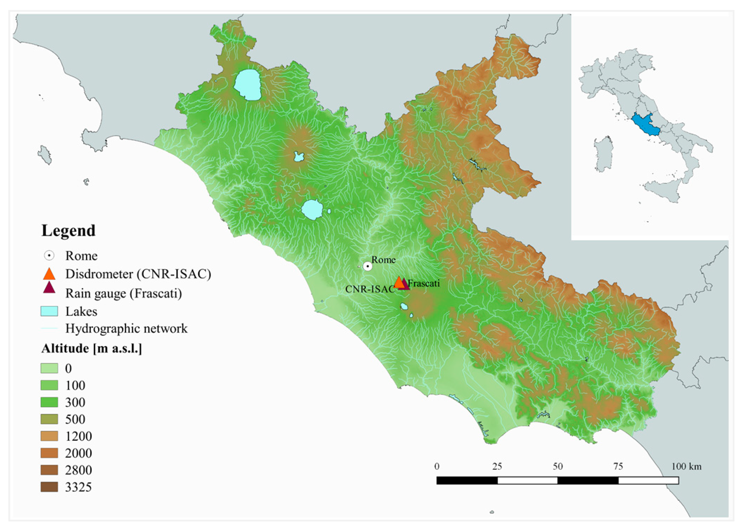
To estimate the kinetic energy of rainfall, we need to investigate the size distribution of raindrops. This can be obtained by direct measurements carried out with pressure transducers, acoustic devices, or disdrometers [33,34]. Performing disdrometric precipitation measurement means determining a pair of velocity–diameter values for each hydrometeor. The relief of dimensional distributions of raindrops was performed with an optical disdrometer, model OTT Parsivel2 (PARticle SIze and VELocity), installed in Rome (central Italy) (Figure 1). The operating principle of the optical disdrometer is based on the measurement of the damping of the light produced by the passage of the drops through a control area of 54 cm2 between two diodes.
The dataset covers a period of about five years, ranging from 20 June 2010 to 28 April 2015. Data gauging time resolution equals 1 min. The Parsivel2 disdrometer classifies drops automatically into 32 separate size classes, ranging from 0.062 to 24.5 mm. However, in this study, Dmax = 7.5 mm was considered as the upper bound for diameter classes, which is consistent with values observed in natural rain [35]. To filter out spurious drops, for each 1 min drop spectrum, the simultaneous presence of 10 drops and a minimum rain rate of 0.01 mmh−1 were selected as thresholds for rain/no-rain events [26]. As a result, 105,433 effective minutes of rain were recorded, with the rainfall intensity varying between 0 and 318.742 mmh−1.
These values were collected for the same time window (i.e., from 20 June 2010 to 28 April 2015). The disdrometer can also record rainfall intensity with a resolution of 0.5 mmh−1. In this regard, as demonstrated in a deep investigation conducted by Adirosi et al. [36], rainfall intensity values collected by a disdrometer can be affected by bias. In this study, this issue was accounted for by filtering the rainfall intensity measured by the disdrometer with the intensity estimated from rainfall drops, as explained below.
2.1. Selection of Potential Erosive Events
Since this methodology aims at defining the relationship between rainfall intensity and kinetic energy which results in soil erosion, we selected erosive rainfall events out of those gauged by the disdrometer according to the classification proposed by Wischmeier and Smith [6]. This method allowed us to exclude events that were not representative for the modeling of soil erosion process. Moreover, raindrops larger than 7.5 mm were excluded from the analysis, since such large measurements can be due either to hail or two or more drops falling at the same moment.
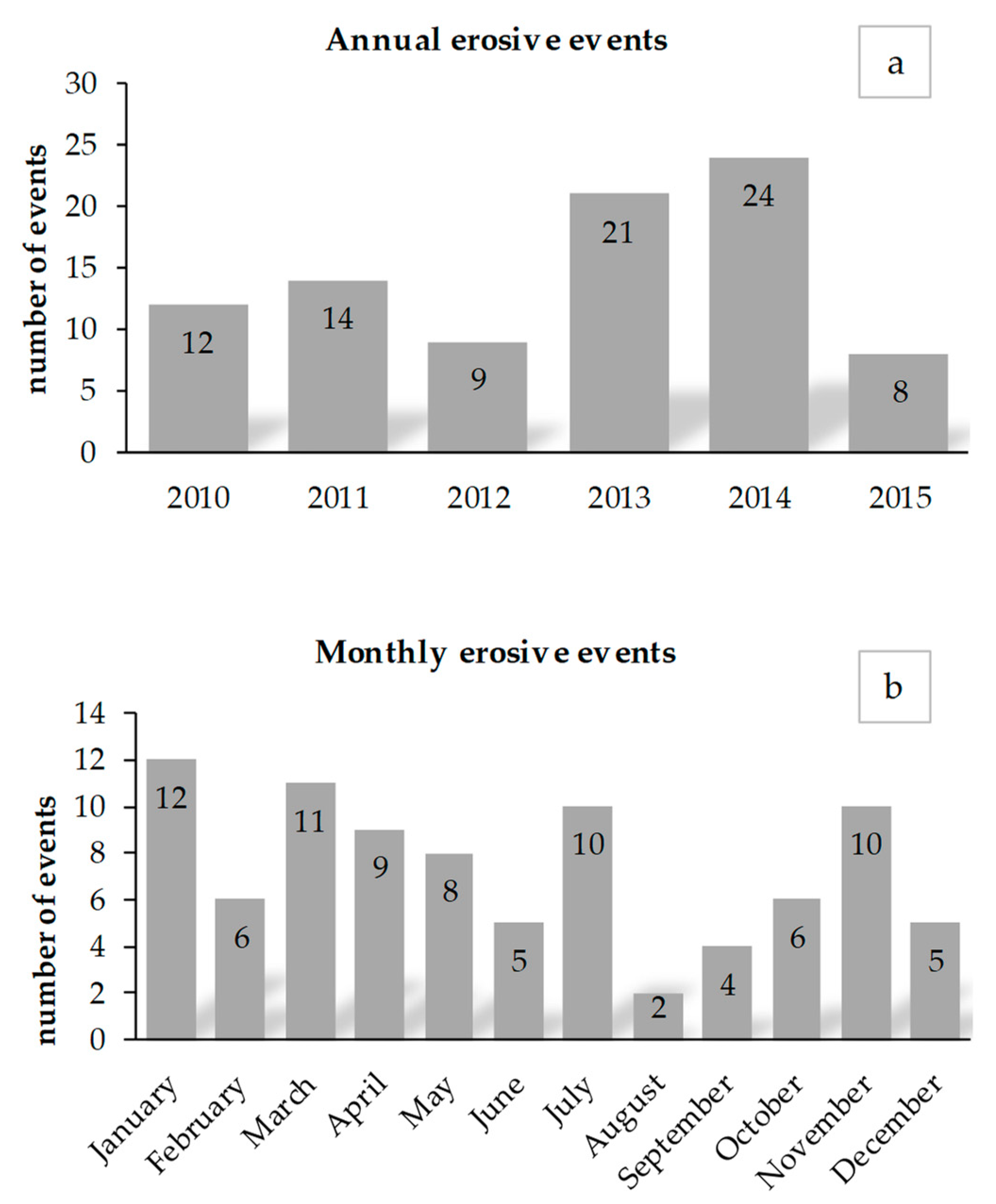
These conditions, applied to our measured drop spectra, led us to identify 88 different events as potentially erosive. The season with the highest number of events (i.e., 28) was spring, while a lower number of events (i.e., 17) occurred in the summer (Figure 2). Based on the annual distribution, the highest number of events occurred in 2014 (Figure 2). In Appendix A, the main characteristics of the erosive events are reported by year of observation.
2.2. Preliminary Analysis of the Dataset
Most erosion control practices are not designed or expected to be proof against extreme events, because in most cases, failure does not cause devastating damages and the practices can be reinstalled without great costs. Thus, in the latest version of the soil loss equation (i.e., RUSLE2 [37]), erosive events with a return period higher than 50 years were removed from R-factor calculations. Therefore, a further investigation was carried out in order to classify the erosive events collected by the disdrometer on the basis of the return period. To this end, we used rainfall depth series recorded by the Frascati rain gauge (18 years of observation), which is the nearest recording station. As is well known, short record lengths can affect the estimation accuracy of high return periods [38]. However, this issue did not play a key role in this investigation. As described below, the relationship between return period and rainfall depth evaluated for the Frascati rain gauge was used only as a threshold, in agreement with Mineo et al. [39].
Rainfall depth precipitation data were collected from 1994 to 2017, which had a 5 min interval time. Then, by aggregation, cumulated rainfall values were obtained for short durations (i.e., 10, 15, 30, 45, and 60 min) and long durations (i.e., 3 and 6 h). For these durations, annual maximum rainfall depths were computed. For the selected station, it was assumed that the rainfall depth values of a specific duration d and return period Tr (i.e., hd,Tr) follow the extreme value type 2 probability distribution law (EV2; [39,40,41]). The three-parameter, site-specific depth–duration–frequency (DDF) curve was adopted [42]:
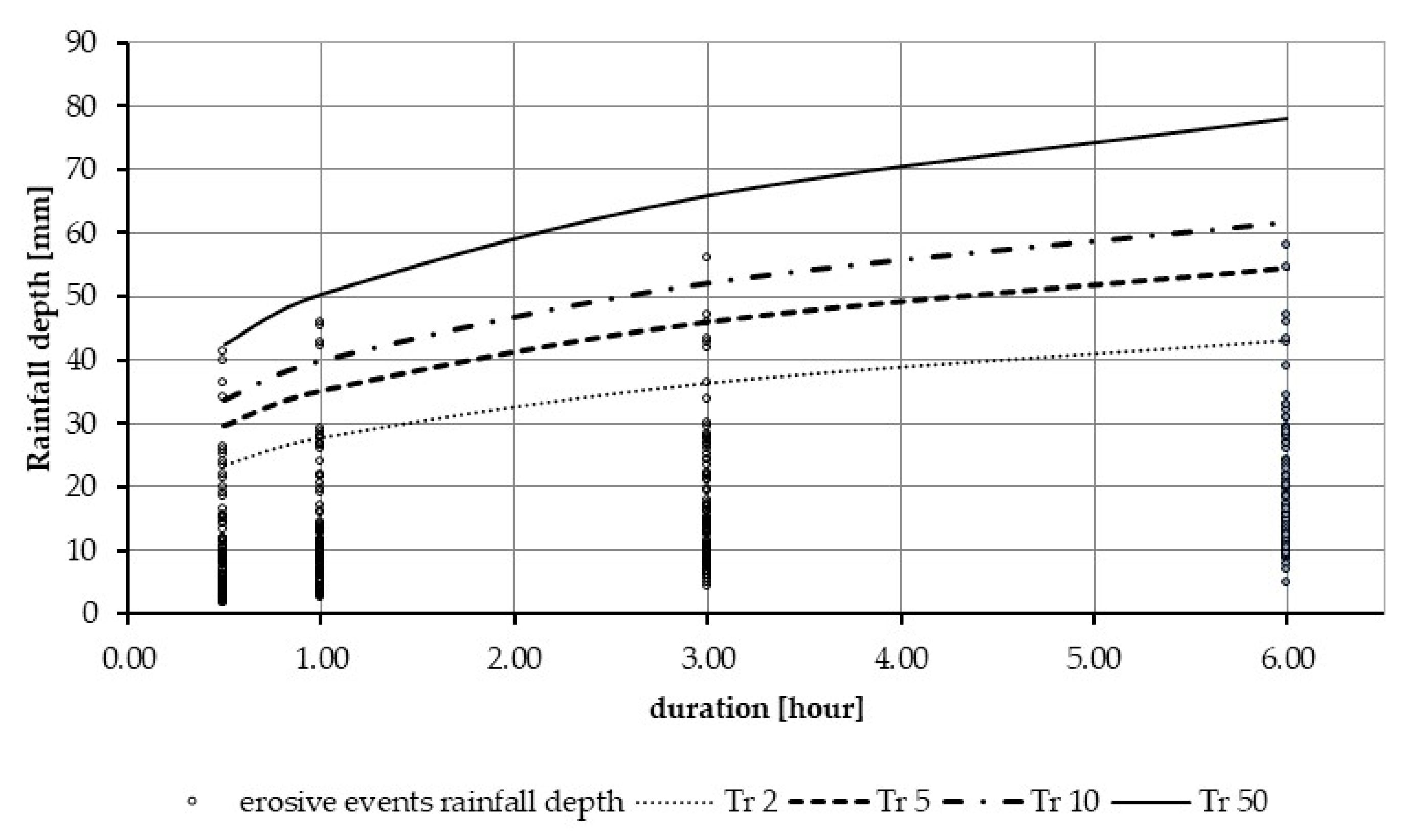
where a and b are positive site-specific parameters, m is an exponent ranging from 0 to 1, and d is the rainfall duration. The parameters were calculated by Mineo and Napolitano [43] by solving Equation (3) numerically. From the DDF curves estimated for the Frascati rain gauge (Figure 3), it was quite evident that potentially erosive events showed depth precipitation amounts lower than the hd,Tr=50yr curve (i.e., no erosive events had a return period higher than 50 years). Therefore, no event was discarded in the subsequent analyses.
In addition, in order to carry out surveys on statistically significant samples [36,40], the following filtering criteria were applied to the measured drop spectra:
- the number of registered drops must be greater than 100;
- at least five raindrops are requested per diameter class;
- rainfall intensity must be greater than 0.5 mmh−1.
Such filtering steps led to a dataset consisting of 28,287 1 min drop spectra.
3. Kinetic Energy Definition
Kinetic energy is the most widely used descriptor of soil erosion. It is estimated evaluating the contribution of all raindrops once their mass, terminal velocity, and DSD are known. The DSD refers to the number of drops present in a unit volume of air (i.e., N(D) (m−3 mm−1)), with a diameter D (mm) ranging between D and D + dD that reaches a unit horizontal area during a unit time Δt (min) [29,44,45,46]. The empirical DSD, for each diameter class k, can be estimated using the following expression [26]:
where ΔDk (mm) is the width of each diameter class, A (m2) is the gauging area of the disdrometer when the ith drop is falling, nt(k) is the number of raindrops falling in the kth class, and Vt(D)k (ms−1) is the raindrop terminal velocity for each kth diameter class.
Kinetic energy is a function of both the mass of raindrops and their terminal velocity. The mass ME (kg) is estimated from the diameters obtained from the DSD and is defined as
where is the water density (1000 kg m−3) under standard conditions. Therefore, once the DSD is known, the mass is estimated from Equation (5). Then, the kinetic energy is half the product of the mass and the terminal velocity of drops at the power of two.
Two expressions of the kinetic energy have been discussed in the literature [9]: the rain kinetic energy rate, or time-specific kinetic energy (i.e., KEtime, expressed in J m−2 h−1), and the rain kinetic energy content, or energy per unit volume (i.e., KEmm, expressed in J m−2 mm−1).
The empirical time-specific kinetic energy is defined as [9]
The empirical rain kinetic energy content KEmm(E) is directly proportional to KEtime(E) by the rain rate I (mmh−1), as shown below:
where c is a constant depending on the unit used. For instance, c equals 1 if KEtime(E) is expressed in J m−2 h−1 and KEmm(E) is in J m−2 mm−1. In Equation (7), empirically evaluating I (i.e., IE, expressed in mm h−1) leads to
It is thus evident that the most important descriptors of the kinetic energy rate are the diameter and the terminal velocity of the drops. The terminal velocity Vt (ms−1) is a function of the drop diameter D (mm). Ulbrich [47] proposed a power law, here denoted as Vt(D)U:
Vt(D)U is thus a monotonically increasing function of the drop diameter. Atlas et al. [48] proposed a formulation interpolating measurements performed by Gunn and Kinzer [49], who estimated the terminal velocity of thousands of artificial droplets with diameter D ranging from 0.2 to 5.8 mm. Atlas et al.’s expression Vt(D)A (ms−1) is as follows:
Equation (10) provides a good fit for diameters larger than 0.4 mm but predicts negative terminal velocity values for very small drops. Finally, Ferro [50] obtained the following relationship considering that terminal velocity is an increasing function (or almost constant for D > 0.55–0.57 cm) of diameter D:
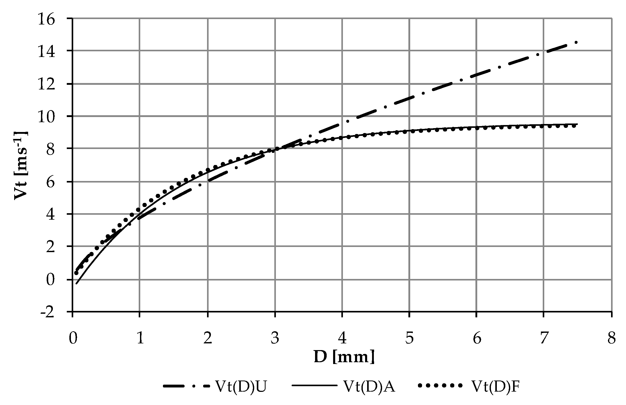
where Vn and an are constants, 9.5 (ms−1) and 6 (cm−1), respectively. Equation (11) was based on the measurements of several scholars [35,49,51,52,53,54]. Vt(D)F equals Vt(D)A for D < 0.55 cm and it is more reliable than Vt(D)U for D > 0.55 cm. According to Ulbrich’s formulation [47], Vt(D)U is monotonically increasing, while Vt(D)A and Vt(D)F tend asymptotically to a constant value (Figure 4).
It is worth noting that, according to the formulations proposed by both [48,50], Vt strongly depends on the diameter for D < 4 mm, while the dependency attenuates for diameters ranging from 4 to 6 mm. For D > 6 mm, the dependency of Vt on D is negligible. In this work, we estimated the terminal velocity according Ferro’s formulation, since Atlas et al.’s relationship inconveniently provides negative values of Vt for small droplet diameters.
KE–I Empirical Relationships
As the formulation of KE is estimated from the DSD, its direct measurement is not always a straightforward task. Therefore, the following approach was used to deal with this issue, that is, the indirect estimation of kinetic energy from another widely measured hydrological variable (i.e., rainfall intensity, I). The advantage of this approach is obvious, given that rain intensity has been measured by rain gauges all over the world [55]. The empirical expressions proposed by different authors reflect different pluviometric calibration regimes through different mathematical formulations that link kinetic energy to precipitation intensity. Henceforth, for the sake of brevity, the relationship between KEmm and I is referred to as KE–I. Several KE–I mathematical relationships proposed in the literature were inspired by the following logarithmic model that implies no upper limit to kinetic energy [6,32]:
where and are constants derived through regression. In a second version of USLE, Wischmeier and Smith [23] showed that kinetic energy does not increase with rainfall intensity indefinitely and proposed a conditional expression (henceforth called WS) on the basis of Equation (12):
It implies that KE remains constant at 28.3 J m−2 mm−1 for rainfall intensity exceeding 76 mmh−1. It was found for Washington (United States) and the DSDs were estimated according to [56].
On the other hand, several authors have proposed an exponential model [11,30,57,58,59,60,61]:
where (J m−2 mm−1), f, and z (h mm−1) are regression parameters. According to Equation (13), Equation (14) leads to an asymptotic value (i.e., KE = γ) at high intensities. Kinnell [59] suggested that the exponential model performs better than the logarithmic one. Having one extra parameter, the exponential model is more flexible to fit the datasets. The developers of RUSLE [7] used Equation (14), with the parameters calibrated by Brown and Foster [30], as a standard method for rainfall energy calculation. Later, in RUSLE2 [37], the exponential model was confirmed, although the method adopts the equation proposed by McGregor et al. [31].
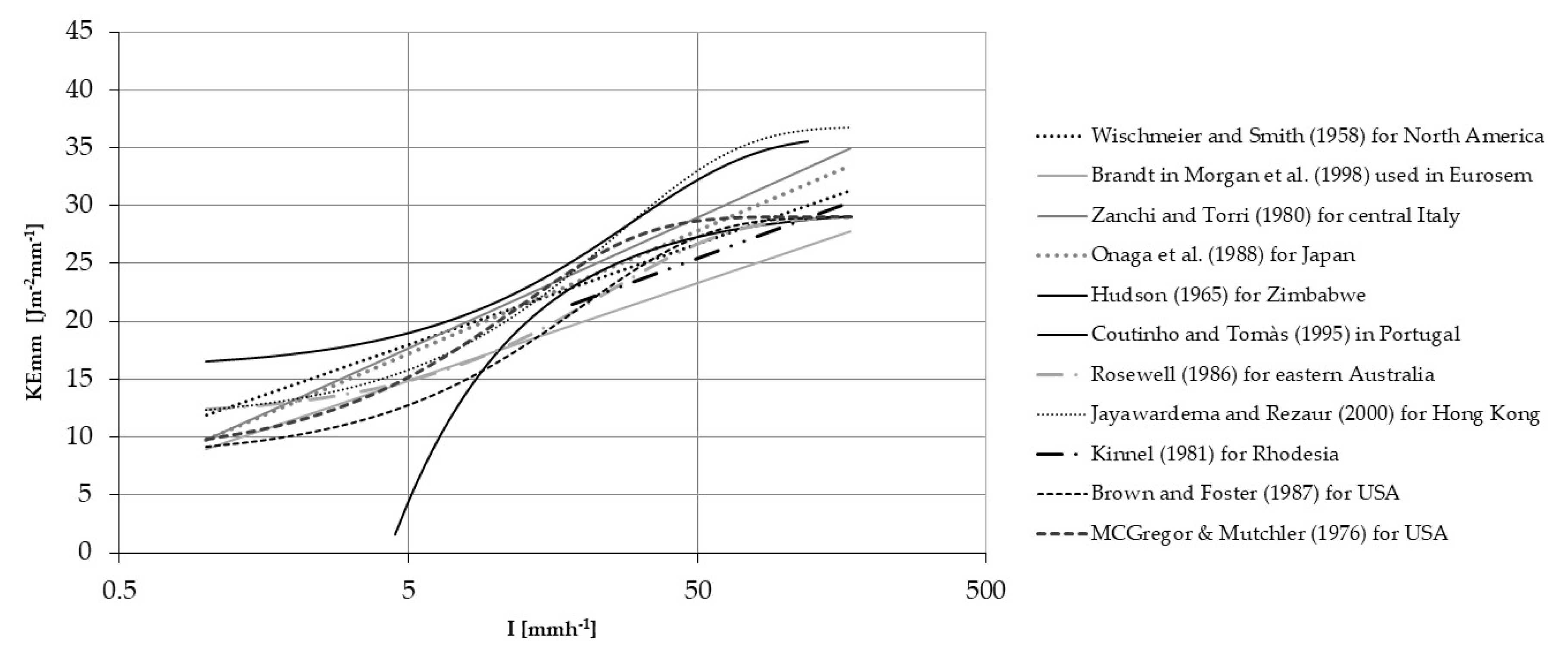
Figure 5 shows some of the expressions found in the literature calibrated for each corresponding pluviometric regime. It is possible to appreciate that the curves tend to overlap for low precipitation intensity values, while the difference between the predicted KE values becomes significant as the intensity increases.
In the 1980s, Zanchi and Torri [32] proposed a relationship (henceforth called ZT) calibrated with measurements performed in Florence (central Italy):
McGregor et al. [31] proposed an equation (henceforth called MG) based on the model suggested by Kinnell [59], which results in
On the other hand, Brown and Foster [30] introduced an exponential relationship (henceforth called BF) for the United States as follows:
4. Results
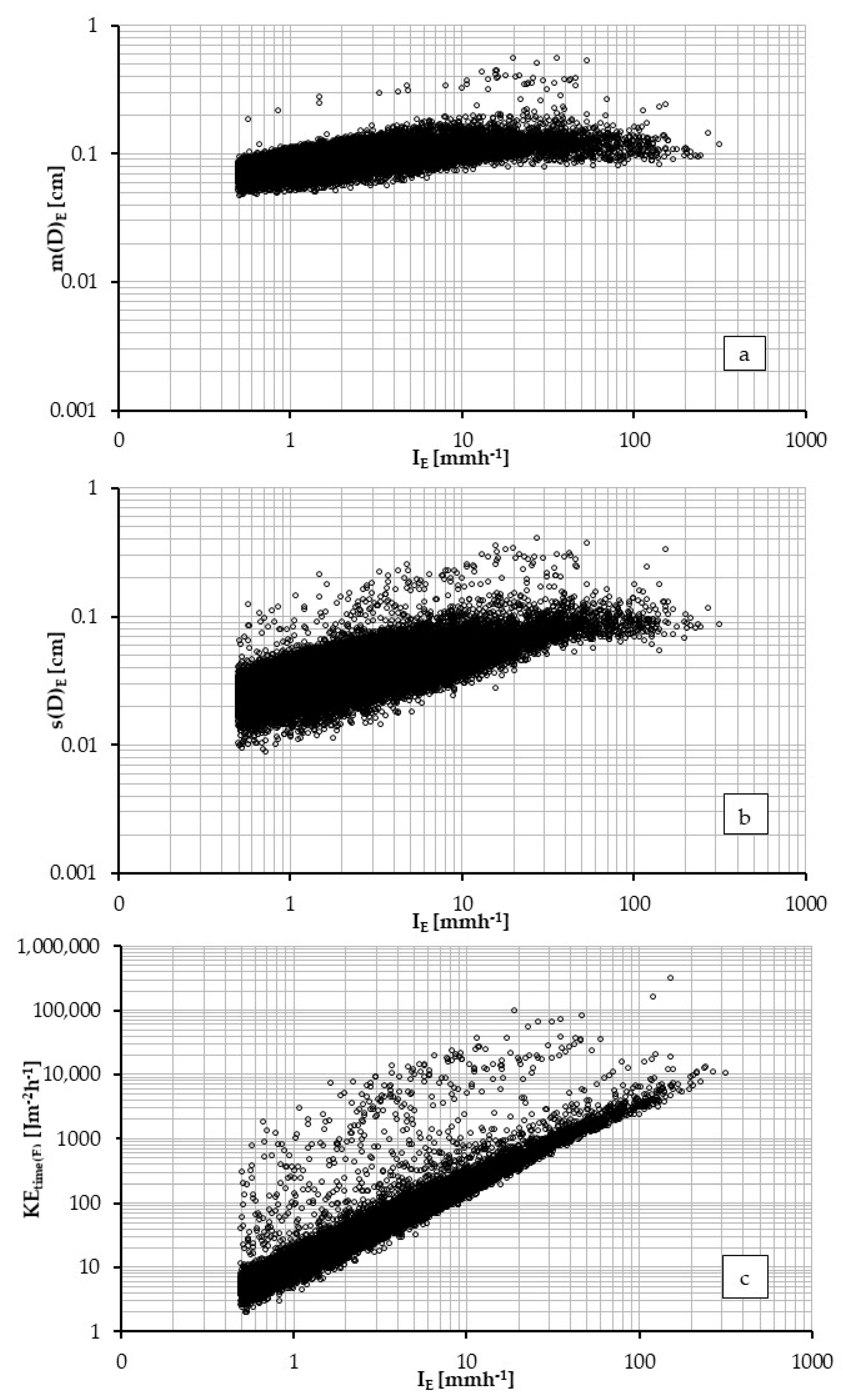
As we used DSDs measured by the disdrometer to estimate the kinetic energy expenditure (i.e., KEtime(E)), the hydrological parameters of interest for the 1 min drop spectra were calculated by summation from the minimum to the maximum diameter collected [26,29]. The empirical DSDs were characterized by rainfall intensity, IE (mmh−1), mean diameter, m(D)E (cm), standard deviation s(D)E (cm), median value of volumetric size spectra D0(E) (cm), and kinetic energy expenditure KEtime(E) (J m−2 h−1). The DSDs identified from the analysis of the 88 selected erosive events were characterized by a mean diameter m(D)E ranging from 0.046 to 0.55 cm and a standard deviation s(D)E from 0.0087 to 0.40 cm. According to what has been found by other authors (e.g., [44]), both the m(D)E and s(D)E of empirical DSDs weakly increase with intensity (Figure 6). In Figure 6a, it is possible to appreciate a range of values of m(D)E that differs significantly from the others. This behavior is even more evident in Figure 6c, where an area that comprises unusually high values of KEtime(E) (even at low intensities) is clearly depicted.
The rationale for this behavior could potentially be due to the horizontal component of wind, as it is one of the main environmental factors that influences disdrometer measurements [1,62]. In fact, the structure of the disdrometer modifies the airflow around the instrument itself and thus affects the trajectories of the falling drops, which can miss the measurement area of the device and not be detected. Friedrich et al. [63] studied the effect of wind on Parsivel2 measurements collected during a hurricane and found that artifacts caused by particles moving at an angle through the sampling area, most of the time, occurred for very strong wind speeds (i.e., more than 20 ms−1), although they were also observed when the wind speed was lower than 10 ms−1. The main effect of the wind is on the number of drops recorded. Another source of error that must be taken into account is splashing, that is, when one drop, hitting the instrument housing, breaks in two drops, which can then enter the measuring area with unrealistically low fall velocities. Wind and splashing effects increase in heavy rain conditions.
Environmental factors (i.e., wind effect and splashing) can therefore cause significant errors in the number of drops recorded by the device, which may not correspond to the intensity value measured by the device (i.e., IM). In fact, the instrument calculates IM regardless of the number of drops recorded, and it can therefore be assumed as a benchmark. Under this assumption, here, we dealt with the environmental factor effects by introducing a further filter on the 1 min drop spectra. Thus, the reliability of the number of drops recorded for each 1 min drop spectrum was assessed by comparing empirical rainfall intensities (IE), calculated using Equation (8), and those registered by the disdrometer (IM). A 1 min drop spectrum was omitted from the analysis if the following condition applied:
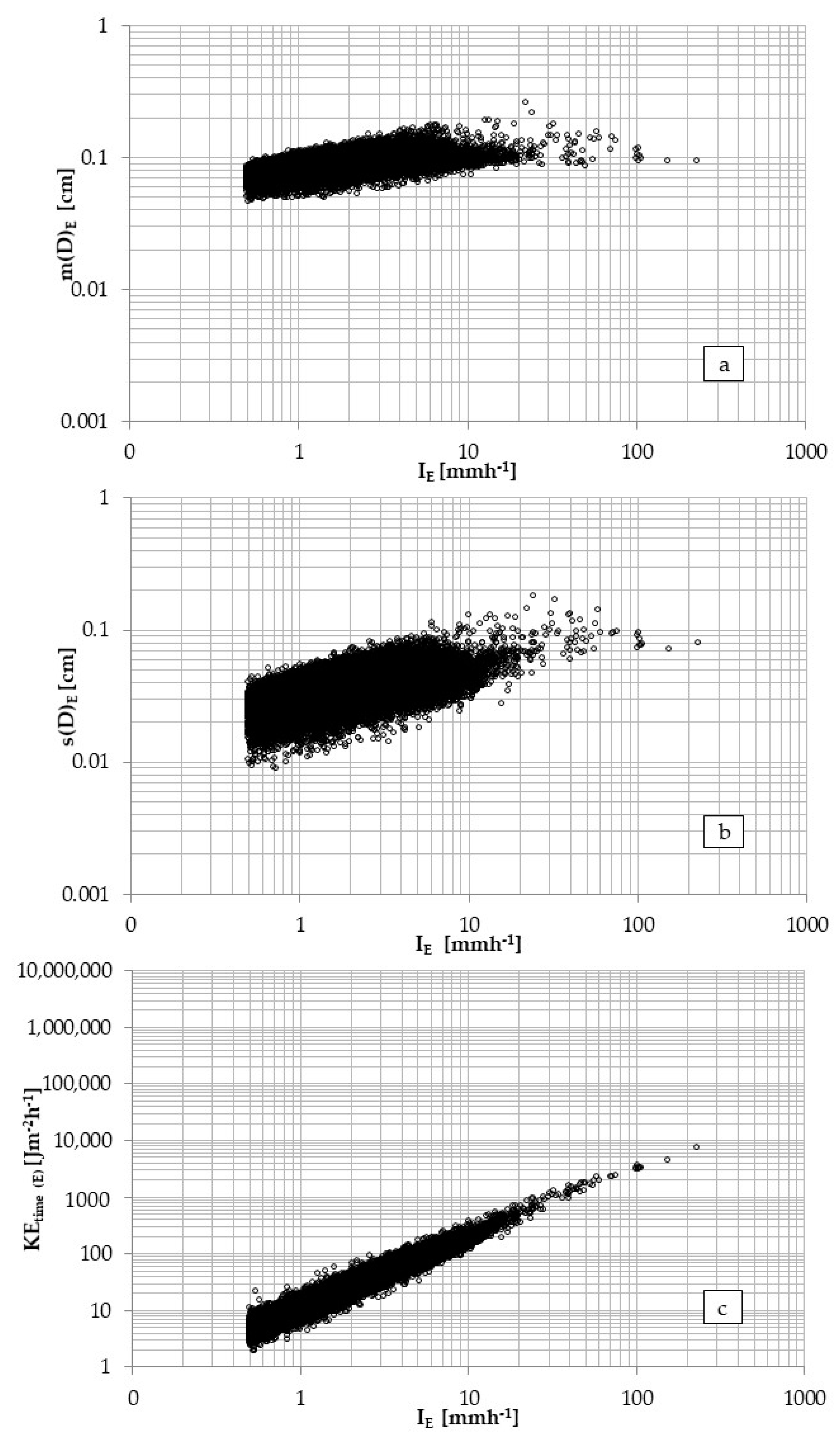
where ∆I is a set equal to 0.5 mmh−1, consistent with device accuracy. This constraint led us to reduce the dataset from 28,284 to 24,330 1 min drop spectra, characterized by
- rainfall intensity, IE, from 0.5 to 230.3 mmh−1;
- mean diameter, m(D)E, from 0.046 to 0.26 cm (Figure 7a);
- standard deviation, s(D)E, from 0.0087 to 0.18 cm (Figure 7b);
- median value of volumetric size spectra, , from 0.042 to 0.49 cm;
- kinetic energy expenditure, KEtime(E), from 1.92 to 7463.8 J m−2 h−1 (Figure 7c).
The elimination of measurements distorted by potential environmental factor effects is more evident when observing the KEtime(E) plotted against the rainfall intensity (Figure 7c). As mentioned, disdrometrical measurements can be affected by different biases; however, it could indeed be that the drop velocity was drastically increased by the wind to cause the scattered KEtime(E) values.
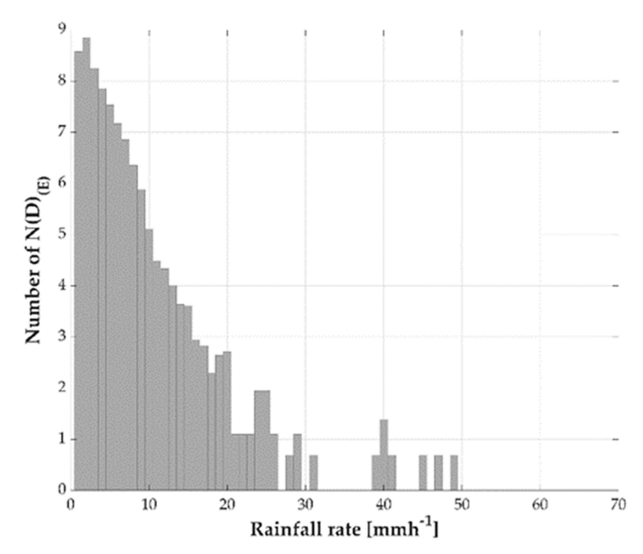
The 24,330 rainfall minutes unfolded in a range of rainfall intensities between 0.5 and 231 mmh−1. However, Figure 8 clearly shows that a high percentile (i.e., 99%) of the drop spectra occurred with a rainfall intensity lower than 15 mmh−1.
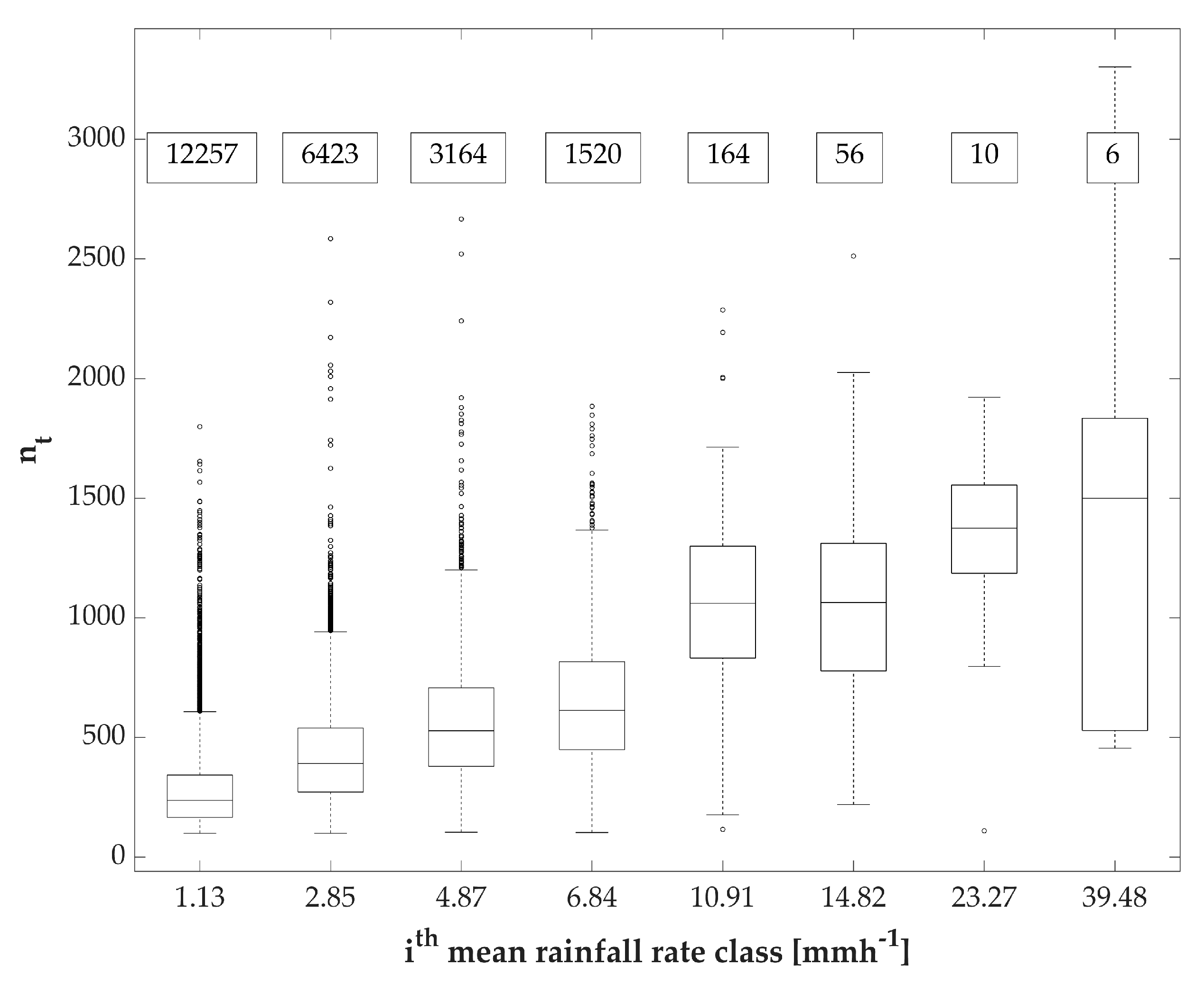
Selecting the 1 min drop spectra by grouping per rainfall rate classes (width of 2 mmh−1), we can observe that (i) the total number of drops falling each minute (i.e., nt) increased with the rainfall intensity, (ii) the range of variability of nt gradually increased with the intensity class, and (iii) the class corresponding to the mean intensity (i.e., 39.48 mmh−1) contained 1 min drop spectra with the highest variability of nt (Figure 9). This suggests that the lower intensity classes consisted of rainfall minutes with more homogeneous characteristics.
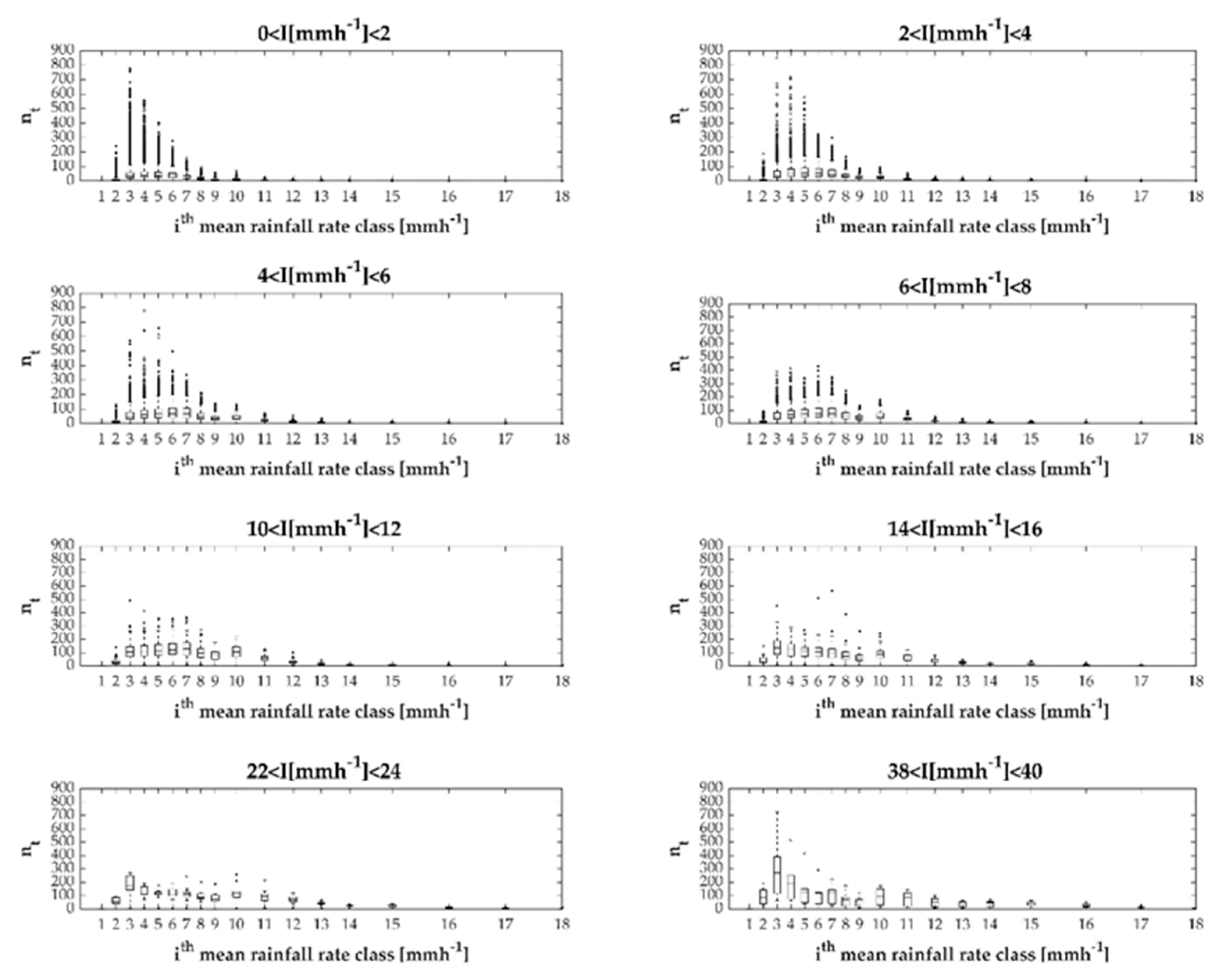
To investigate the link between the number of drops and rainfall intensity more deeply, in Figure 10, the box plots for j different intensity classes (with j = 8) are depicted. In each plot, the number of drops falling in eight out of the nt(k) diametrical classes are shown for each 1 min drop spectrum. Figure 10 suggests the following considerations: (i) the median value of nt(k)(j) assumes greater values as the jth intensity class increases; (ii) for intensity classes lower than 14 mmh−1, the maximum median value nt(k)(j)max shifts towards greater diametrical classes as the jth class intensity increases; (iii) for intensity classes greater than 14 mmh−1, the nt(k)(j)max shifts towards smaller diametrical classes as the jth intensity class increases.
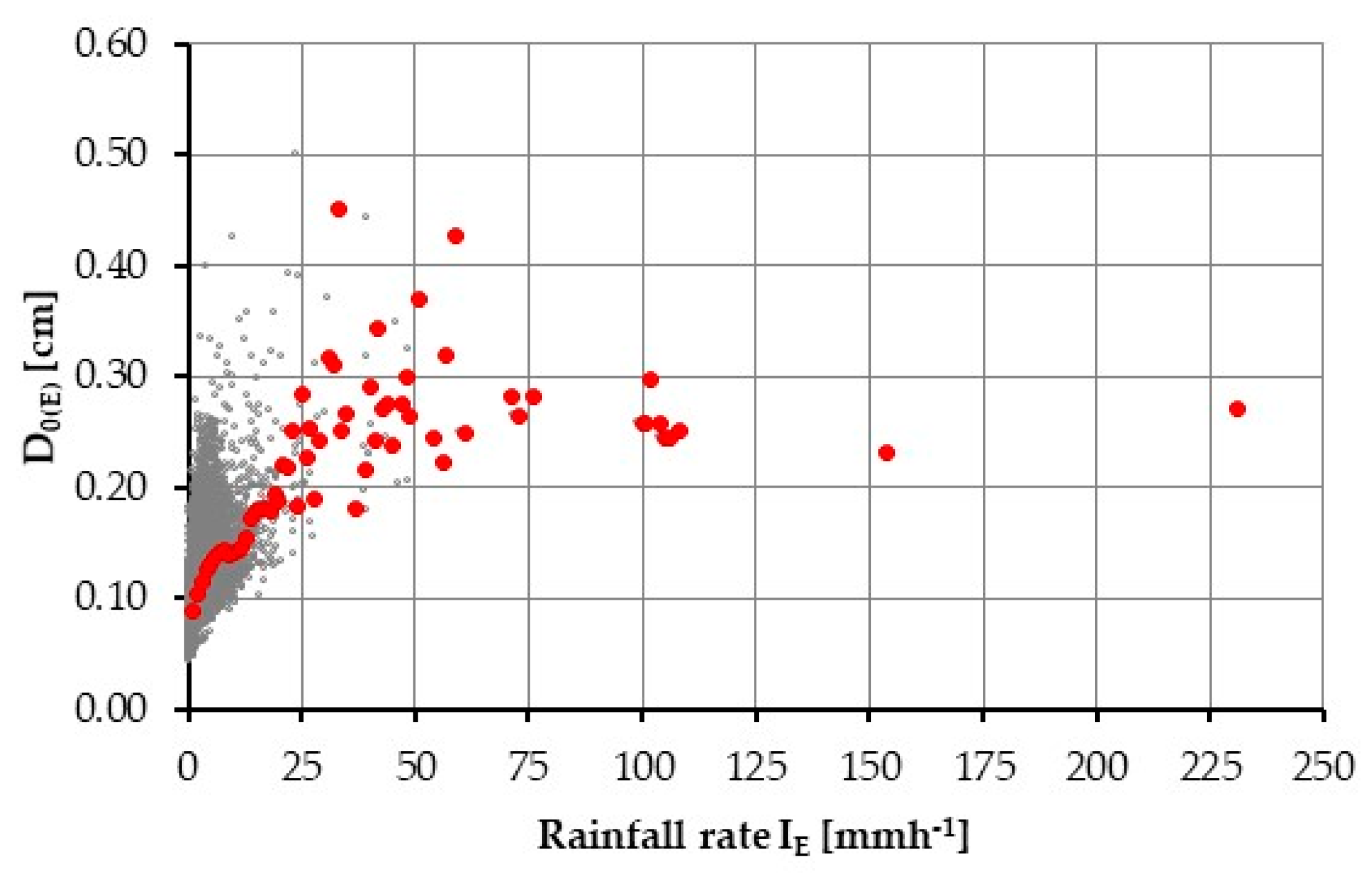
The results suggest that, for low intensity classes, there was a prevalence of droplets (i.e., drops with a diameter of <1 mm). As the intensity increased, the number of large diameter drops increased, and the coalescence phenomenon was prevalent, while the percentage of droplets decreased progressively and then grew again at a specific threshold value. This trend can be explained by the fact that the larger drops, which become unstable, start to break into smaller drops (i.e., disaggregation), determining quasi-constant values of the empirical median volume diameter (Figure 11) and kinetic energy content (Figure 12) as well [11,60].
Regarding the investigated drop spectra, the maximum values of D0(E) (Figure 11) and KEmm(E) (Figure 12) were achieved at an intensity threshold of 32 mmh−1. This result confirms the approach proposed by Wischmeier and Smith [23], which found a limit value of 76 mmh−1, calibrated on the U.S. pluviometric regime. Different limit values were assessed for different case studies by other authors, for instance, Rosewell [60] found a value of 100 mmh−1 in Australia, while Carollo et al. [44] found that this value is equal to 40 mmh−1 for the Sicilian pluviometric regime.
5. Discussion: A New Analytical Relationship
Since this paper is focused on processes on the earth’s surface, it is of primary importance that proper estimates are obtained for KE values at higher rainfall intensities.
To determine the most suitable KE–I relationship for the case study under analysis, the relationship existing between kinetic energy and empirical drop size distributions (i.e., number of drops vs. rainfall intensity) was investigated. Using Equation (7) and the expression proposed by Ferro [50] to estimate terminal velocity (i.e., Equation (11)), we estimated KEmm(E) from disdrometer measurements. KEmm(E) was estimated and then plotted against rainfall intensity.
Figure 13 shows the comparison between pairs of KEmm(E) mean values and IM, and pairs of KE–I predicted by WS, ZT, MG, and BF relationships. We can clearly see the different trend of the ZT equation (green line), as it does not consider a threshold value for intensity.
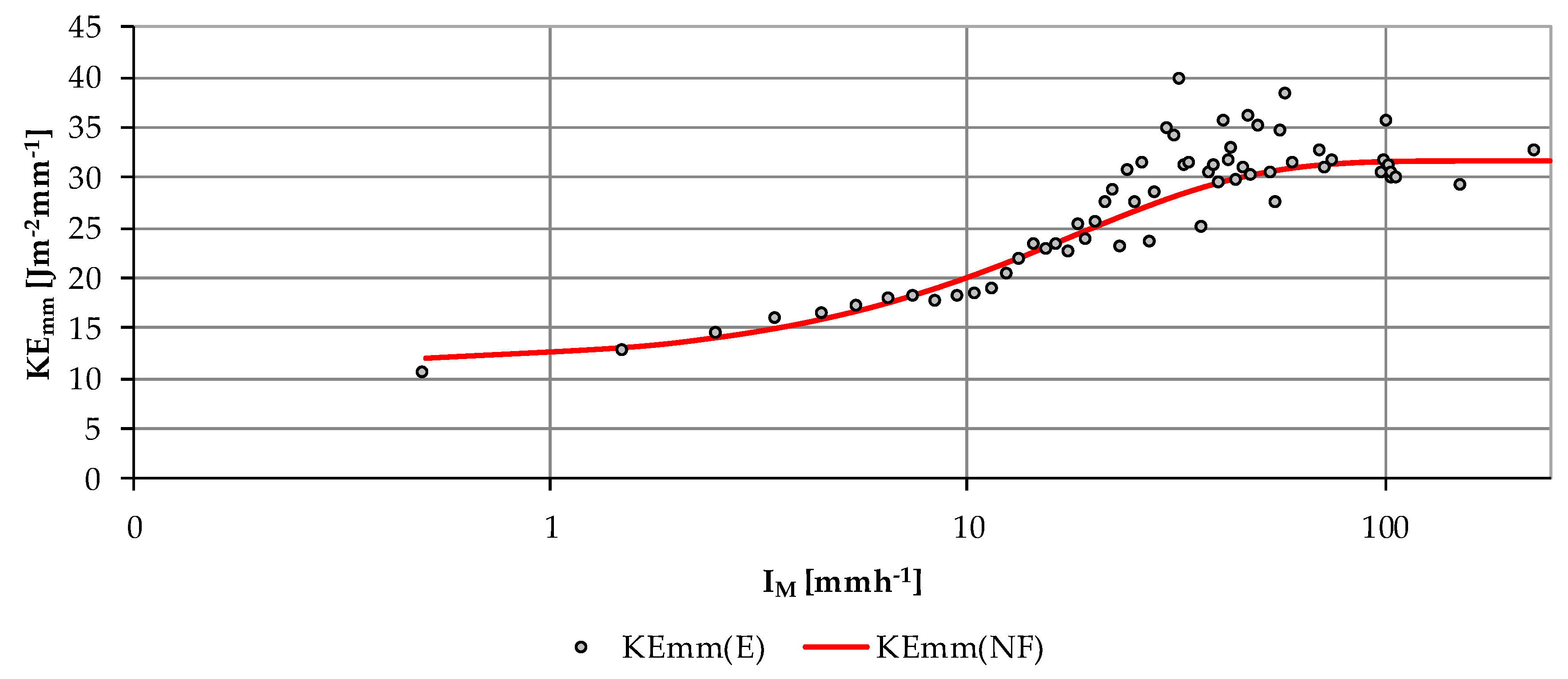
Finally, recalibrating the rainfall energy equation proposed by Kinnel [59], a relationship relating KEmm and I here was derived through regression analysis:
The equation better represents the KE–I trend over the area of the case study (Figure 14).
To estimate the goodness of fit of the analytical relations, the mean absolute percentage error (MAPE, %), the root-mean-square error (RMSE, J m−2 mm−1), and the normalized RMSE (NRMSE, dimensionless) were evaluated:
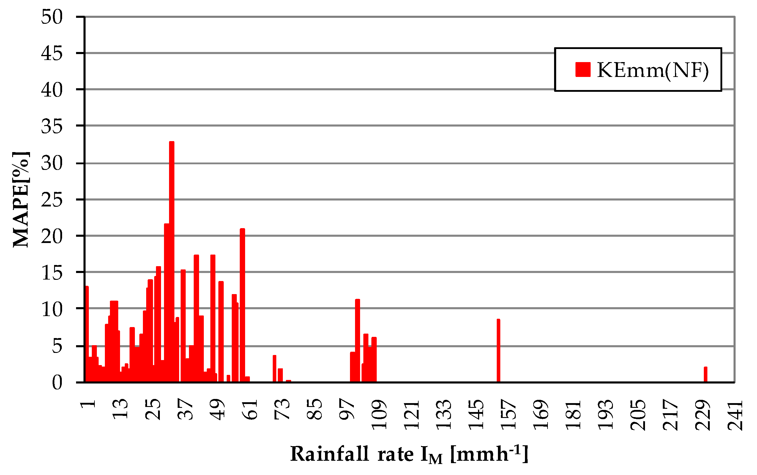
where KE(model),i is represented by the ith values of rainfall kinetic energy predicted by both the literature empirical formulations (WS, ZT, BF, and MG) and by Equation (19) (hereinafter KEmm(NF) or new formulation). In Figure 15, the MAPE (Equation (20)) between the KEmm(E) and the ones predicted by empirical formulations (WS, ZT, BF, and MG) are represented, depending on rainfall intensity.
In terms of lowest MAPE, among the expressions in the literature, the best performance was provided by MG, followed by ZT. The greatest percentage values of MAPE were obtained by comparing the values of KEmm(E) with the expression from BF. Certainly, the best performance was provided by the relationship specifically recalibrated for the case study (Figure 16 and Table 1). Therefore, even if a reasonable dispersion between KEmm(E) and KEmm(NF) is appreciable, Equation (19) offers an improvement compared with the other literature expressions. Therefore, for the case study, the results suggest that the new formulation is preferable to calculate the kinetic energy of precipitation.
However, it is important to highlight that, among the other formulations, the best performance was provided by MG´s expression. This is extremely interesting, since this relationship is used to estimate the RUSLE2, which is the most updated expression to estimate soil erosion and its use is widespread. The fact that MG´s expression could successfully describe the pluviometric regime under study highlights its robustness and its wide range of applicability. Once its suitability to a case study area is verified, it could be used in ungauged areas or in case of missing data. However, if data are available, the new relationship proposed here can be an effective replacement of MG´s expression.
6. Conclusions
In this paper, first, we estimated kinetic energy values from measurements of an optical disdrometer installed in Rome. Then, we assessed the performance of some literature relationships which have had a major role in the estimation of the R-factor in the RUSLE equation and its further updates: the relationships proposed by Wischmeier and Smith [6], used in USLE; Brown and Foster [30] (RUSLE); and McGregor et al. [31] (RUSLE2). The relationship proposed by Zanchi and Torri [32] was also assessed, as it was estimated from data collected in central Italy.
From analyzing the kinetic energy against the rainfall intensity obtained from data collected by the disdrometer, it was evident that a large portion of data was scattered and did not cluster with the rest of the data. While in usual practice these data are kept in the analysis, here, these measurements, likely distorted by the side wind effect, were eliminated to retrieve a proper KE–I relationship. From the measurements, for large values of rainfall intensity, the empirical kinetic energy content of rainfall had quasi-constant values. This was due to the fact that the larger drops, which became unstable, broke into smaller drops (i.e., disaggregation), determining quasi-constant values of the empirical median volume diameter. The maximum values of the energy of raindrops were quasi-constant at intensities exceeding 32 mmh−1. This finding confirms what was found by many authors who established a limit value that varies with the pluviometric regime and, thus, with the case study.
From the analysis, it was thus clear that the KE–I relationship was strongly influenced by the pluviometric regime under study. Therefore, it was necessary to assess if KE–I literature expressions are suitable for the case study under analysis (i.e., Rome). Among literature expressions, the best performance was provided by McGregor et al.’s [31] expression, followed by Zanchi and Torri [32]. This has an important implication, since McGregor et al.’s [31] relationship is used in the framework of the RUSLE2, which is the most updated expression to estimate soil erosion and is used worldwide. Instead, the greatest percentile values of error were found by comparing the empirical values of KEmm with the expression from Brown and Foster [30]. Finally, an exponential equation relating kinetic energy and rainfall intensity was recalibrated in order to better represent the KE–I trend over the case study. The application of a local kinetic energy expression resulted in, on average, the best performance in estimating the kinetic energy values, as compared with the equations proposed by the RUSLE manual, which were not developed specifically for the Lazio region. Even if a reasonable dispersion between empirical values of kinetic energy and those obtained with the new relationship is appreciable, the new relationship offers an improvement in the estimation of KEmm. Since the results led us to verify that the McGregor et al. [31] expression is suitable to describe the pluviometric regime under study, in case of an ungauged area or missing data, it can also be used to estimate the kinetic energy for the case study area. However, if data are available, the new relationship proposed in this paper can be an effective replacement of McGregor et al.’s [31] expression for the case study area.
Author Contributions
Conceptualization, C.M., F.R., and F.N.; methodology, C.M., E.R., F.R., and F.N.; formal analysis, C.M. and B.M.; data curation, C.M.; writing—original draft preparation, E.R. and C.M.; writing—review and editing, C.M., E.R., and B.M.; supervision, F.R. and F.N.
Funding
This research received no external funding.
Acknowledgments
The authors acknowledge the CNR-ISAC and the Servizio Idrografico e Mareografico of Regione Lazio for providing the disdrometer and the rainfall dataset, respectively. The authors are also grateful to Federica Astrologo for her precious contribution in a preliminary analysis of the dataset.
Conflicts of Interest
The authors declare no conflict of interest.
Appendix A
Table A1 shows the main characteristics of the erosive events identified according to the methodology proposed by Wischmeier and Smith [61], reported by year of observation. For each event, we reported the duration; the rainfall depth recorded at 5, 15, 30, 60, 180, and 360 min; and the total rainfall depth amount.

Table A1.
Basic characteristics of the potential erosive events considered in this study, calculated using a moving window for each time interval.
Table A1.
Basic characteristics of the potential erosive events considered in this study, calculated using a moving window for each time interval.
| Event | Date | Duration | 5 min | 15 min | 30 min | 60 min | 180 min | 360 min | Total Depth |
|---|---|---|---|---|---|---|---|---|---|
| (DD/MM/YYYY) | (min) | (mm) | (mm) | (mm) | (mm) | (mm) | (mm) | (mm) | |
| 1 | 26/06/2010 | 503 | 12.26 | 21.58 | 26.07 | 26.45 | 26.53 | 26.77 | 26.87 |
| 2 | 08/09/2010 | 88 | 14.26 | 24.05 | 25.55 | 25.84 | 25.85 | 25.85 | 25.85 |
| 3 | 05/10/2010 | 138 | 15.57 | 23.88 | 23.90 | 23.96 | 24.20 | 24.20 | 24.20 |
| 4 | 13/10/2010 | 596 | 2.77 | 6.04 | 9.69 | 11.27 | 13.00 | 20.27 | 20.77 |
| 5 | 31/10/2010 | 2777 | 7.37 | 12.36 | 14.48 | 19.40 | 29.88 | 30.72 | 41.02 |
| 6 | 07/11/2010 | 3610 | 2.00 | 2.22 | 2.67 | 5.07 | 8.43 | 10.15 | 28.21 |
| 7 | 10/11/2010 | 209 | 6.71 | 9.72 | 11.23 | 11.23 | 13.15 | 13.27 | 13.27 |
| 8 | 18/11/2010 | 2290 | 1.99 | 2.10 | 2.74 | 3.20 | 5.48 | 9.68 | 13.11 |
| 9 | 21/11/2010 | 3206 | 3.46 | 4.44 | 8.06 | 11.82 | 15.26 | 18.58 | 46.83 |
| 10 | 02/12/2010 | 851 | 2.72 | 3.05 | 3.16 | 3.76 | 7.50 | 9.84 | 13.04 |
| 11 | 17/12/2010 | 1084 | 1.89 | 3.49 | 5.13 | 8.56 | 16.13 | 23.97 | 39.72 |
| 12 | 23/12/2010 | 3443 | 4.27 | 6.48 | 8.50 | 9.60 | 16.06 | 18.63 | 61.92 |
| 13 | 21/01/2011 | 2030 | 2.04 | 2.67 | 2.87 | 3.07 | 6.55 | 9.21 | 23.55 |
| 14 | 30/01/2011 | 1256 | 1.59 | 2.84 | 4.36 | 6.25 | 7.21 | 8.94 | 12.72 |
| 15 | 16/02/2011 | 1513 | 1.05 | 1.64 | 2.27 | 4.15 | 8.65 | 13.08 | 15.77 |
| 16 | 01/03/2011 | 3893 | 1.00 | 2.17 | 3.27 | 5.90 | 11.56 | 14.50 | 42.14 |
| 17 | 16/03/2011 | 1457 | 3.83 | 7.87 | 10.20 | 12.97 | 24.89 | 31.86 | 68.58 |
| 18 | 17/03/2011 | 1050 | 3.66 | 6.29 | 9.18 | 11.56 | 14.23 | 15.92 | 28.71 |
| 19 | 25/04/2011 | 1195 | 0.89 | 2.22 | 3.72 | 7.11 | 9.61 | 9.62 | 12.89 |
| 20 | 27/04/2011 | 354 | 1.87 | 3.62 | 5.74 | 9.35 | 13.95 | 15.05 | 15.05 |
| 21 | 02/05/2011 | 506 | 1.14 | 2.57 | 4.81 | 8.86 | 14.62 | 15.47 | 15.92 |
| 22 | 03/05/2011 | 219 | 6.50 | 7.79 | 7.93 | 8.00 | 8.08 | 8.43 | 8.43 |
| 23 | 16/05/2011 | 347 | 5.48 | 12.03 | 15.62 | 19.07 | 21.84 | 21.85 | 21.85 |
| 24 | 05/07/2011 | 163 | 13.94 | 23.99 | 39.70 | 45.17 | 45.96 | 45.96 | 45.96 |
| 25 | 27/07/2011 | 646 | 12.45 | 18.93 | 21.75 | 27.98 | 33.76 | 34.38 | 38.18 |
| 26 | 19/10/2011 | 757 | 6.99 | 11.90 | 18.38 | 28.39 | 55.79 | 58.00 | 58.13 |
| 27 | 19/04/2012 | 1212 | 2.46 | 2.69 | 3.07 | 5.36 | 7.94 | 10.47 | 15.69 |
| 28 | 06/05/2012 | 1886 | 1.19 | 1.76 | 2.58 | 2.89 | 4.72 | 4.93 | 14.86 |
| 29 | 21/05/2012 | 1200 | 2.53 | 4.10 | 5.64 | 6.94 | 10.68 | 16.91 | 39.33 |
| 30 | 12/09/201 | 1162 | 8.29 | 8.67 | 8.72 | 8.72 | 8.77 | 16.85 | 20.79 |
| 31 | 14/09/2012 | 939 | 0.88 | 1.79 | 3.30 | 4.68 | 9.65 | 13.61 | 15.46 |
| 32 | 30/09/2012 | 1130 | 1.53 | 1.86 | 2.33 | 4.36 | 9.08 | 13.26 | 17.56 |
| 33 | 28/11/2012 | 3096 | 2.31 | 3.08 | 3.09 | 3.97 | 7.69 | 13.37 | 54.20 |
| 34 | 07/12/2012 | 926 | 1.60 | 3.30 | 4.67 | 6.10 | 10.92 | 14.55 | 18.08 |
| 35 | 26/12/2012 | 394 | 5.11 | 11.82 | 15.18 | 16.86 | 17.33 | 17.33 | 17.35 |
| 36 | 13/01/2013 | 2209 | 3.28 | 3.65 | 4.89 | 8.01 | 17.70 | 18.22 | 28.99 |
| 37 | 15/01/2013 | 1688 | 1.39 | 3.29 | 5.82 | 10.04 | 16.93 | 19.49 | 33.38 |
| 38 | 19/01/2013 | 3085 | 0.77 | 1.66 | 2.63 | 4.23 | 5.86 | 7.77 | 24.35 |
| 39 | 11//2/2013 | 1190 | 2.23 | 4.59 | 6.84 | 11.53 | 24.04 | 30.71 | 35.12 |
| 40 | 23/02/2013 | 3463 | 3.51 | 5.40 | 8.32 | 12.80 | 19.60 | 28.18 | 66.05 |
| 41 | 06/03/2013 | 1089 | 0.45 | 0.98 | 1.59 | 2.74 | 6.46 | 8.99 | 12.86 |
| 42 | 11/03/2013 | 1521 | 0.90 | 1.59 | 2.28 | 3.79 | 6.68 | 9.31 | 17.03 |
| 43 | 25/03/2013 | 638 | 2.60 | 4.66 | 8.15 | 10.71 | 14.59 | 14.70 | 15.06 |
| 44 | 30/03/2013 | 793 | 2.07 | 4.14 | 5.30 | 8.11 | 10.56 | 10.96 | 13.98 |
| 45 | 01/04/2013 | 1628 | 10.52 | 16.00 | 18.92 | 21.58 | 27.76 | 32.75 | 44.92 |
| 46 | 21/04/2013 | 1389 | 0.96 | 1.58 | 2.53 | 3.51 | 4.29 | 6.84 | 13.00 |
| 47 | 06/05/2013 | 785 | 8.51 | 13.43 | 16.32 | 26.54 | 36.32 | 39.00 | 41.36 |
| 48 | 22/05/2013 | 1699 | 2.48 | 5.37 | 8.02 | 12.94 | 14.90 | 18.42 | 23.18 |
| 49 | 01/06/2013 | 748 | 3.67 | 8.25 | 10.43 | 12.50 | 14.27 | 14.28 | 14.37 |
| 50 | 04/06/2013 | 1229 | 7.38 | 8.93 | 8.99 | 9.01 | 9.31 | 9.59 | 9.67 |
| 51 | 28/06/2013 | 77 | 10.44 | 13.85 | 14.83 | 26.74 | 26.88 | 26.88 | 26.88 |
| 52 | 04/07/2013 | 74 | 5.98 | 12.65 | 23.27 | 29.17 | 29.30 | 29.30 | 29.30 |
| 53 | 08/07/2013 | 170 | 10.26 | 19.04 | 19.80 | 20.34 | 20.91 | 20.91 | 20.91 |
| 54 | 10/07/2013 | 227 | 4.73 | 6.99 | 7.65 | 7.68 | 8.48 | 8.77 | 8.77 |
| 55 | 20/08/2013 | 166 | 13.27 | 31.56 | 41.2 | 45.91 | 47.09 | 47.09 | 47.09 |
| 56 | 25/08/2013 | 109 | 11.36 | 23.45 | 34.04 | 42.02 | 42.75 | 42.75 | 42.75 |
| 57 | 14/01/2014 | 654 | 1.19 | 2.26 | 3.75 | 5.98 | 10.10 | 13.06 | 13.86 |
| 58 | 19/01/2014 | 2434 | 5.50 | 8.08 | 8.59 | 8.60 | 14.32 | 19.81 | 37.86 |
| 59 | 23/01/2014 | 1298 | 1.04 | 1.77 | 2.46 | 4.36 | 7.78 | 10.96 | 13.29 |
| 60 | 29/11/2014 | 1512 | 1.39 | 1.76 | 2.64 | 3.58 | 6.59 | 10.45 | 14.18 |
| 61 | 31/01/2014 | 5885 | 3.49 | 4.59 | 6.86 | 11.47 | 19.13 | 28.94 | 103.23 |
| 62 | 05/02/2014 | 1723 | 0.84 | 1.26 | 2.02 | 3.37 | 7.77 | 9.13 | 13.06 |
| 63 | 28/02/2014 | 2334 | 2.19 | 4.75 | 9.14 | 14.34 | 27.31 | 32.92 | 54.31 |
| 64 | 03/03/2014 | 1093 | 1.55 | 3.18 | 4.64 | 6.41 | 11.28 | 11.44 | 15.36 |
| 65 | 04/04/2014 | 260 | 5.81 | 9.00 | 11.64 | 12.87 | 13.73 | 13.89 | 13.89 |
| 66 | 19/04/2014 | 1124 | 3.77 | 8.94 | 11.70 | 13.99 | 14.35 | 14.53 | 16.54 |
| 67 | 02/05/2014 | 2024 | 3.55 | 8.05 | 11.58 | 13.50 | 22.10 | 27.55 | 47.43 |
| 68 | 27/06/2014 | 46 | 10.50 | 12.70 | 13.15 | 13.85 | 13.85 | 13.85 | 13.85 |
| 69 | 10/07/2014 | 22 | 7.21 | 10.36 | 10.50 | 10.50 | 10.50 | 10.50 | 10.50 |
| 70 | 13/07/2014 | 419 | 3.71 | 6.18 | 8.20 | 13.10 | 13.66 | 15.48 | 20.69 |
| 71 | 17/07/2014 | 285 | 11.74 | 20.44 | 21.31 | 21.45 | 21.60 | 21.60 | 21.60 |
| 72 | 22/07/2014 | 519 | 1.82 | 2.62 | 3.77 | 6.28 | 9.96 | 12.20 | 15.40 |
| 73 | 29/07/2014 | 652 | 4.47 | 8.87 | 9.43 | 15.79 | 23.24 | 23.24 | 35.01 |
| 74 | 01/10/2014 | 313 | 5.35 | 9.40 | 11.64 | 12.99 | 13.03 | 13.06 | 13.06 |
| 75 | 02/10/2014 | 91 | 18.01 | 29.57 | 36.40 | 42.53 | 43.30 | 43.30 | 43.30 |
| 76 | 03/10/2014 | 221 | 8.51 | 12.64 | 15.35 | 16.02 | 16.02 | 16.29 | 16.29 |
| 77 | 06/11/2014 | 1319 | 9.51 | 17.16 | 25.14 | 27.68 | 41.76 | 54.63 | 128.22 |
| 78 | 12/11/2014 | 703 | 0.96 | 2.38 | 4.26 | 6.09 | 8.22 | 11.12 | 20.32 |
| 79 | 15/11/2014 | 522 | 9.12 | 11.80 | 14.03 | 21.92 | 28.01 | 28.03 | 28.04 |
| 80 | 16/11/2014 | 902 | 3.34 | 6.25 | 7.71 | 9.89 | 12.19 | 12.48 | 18.16 |
| 81 | 19/01/2015 | 1361 | 0.56 | 1.03 | 1.53 | 2.38 | 6.10 | 9.57 | 14.90 |
| 82 | 21/01/2105 | 2501 | 1.00 | 2.16 | 4.00 | 6.47 | 8.62 | 11.76 | 16.22 |
| 83 | 29/01/2015 | 3505 | 1.13 | 2.32 | 3.44 | 4.28 | 8.00 | 12.36 | 26.00 |
| 84 | 03/02/2015 | 4438 | 2.83 | 4.74 | 6.69 | 8.43 | 12.49 | 20.12 | 66.66 |
| 85 | 04/03/2015 | 1387 | 1.10 | 2.58 | 4.24 | 7.09 | 16.57 | 22.68 | 45.52 |
| 86 | 25/03/2015 | 1296 | 1.48 | 3.42 | 6.30 | 10.82 | 20.99 | 28.99 | 57.86 |
| 87 | 04/04/2015 | 1730 | 2.77 | 4.80 | 6.08 | 6.72 | 9.63 | 10.22 | 19.20 |
| 88 | 27/04/2015 | 2456 | 2.68 | 5.10 | 8.35 | 11.30 | 28.23 | 28.48 | 51.01 |
References
- Fornis, R.L.; Vermeulen, H.R.; Nieuwenhuis, J.D. Kinetic energy-rainfall intensity relationship for Central Cebu, Philippines for soil erosion studies. J. Hydrol. 2005, 300, 20–32. [Google Scholar] [CrossRef]
- Pimentel, D.; Harvey, C.; Resosudarmo, P.; Sinclair, K.; Kurz, D.; McNair, M.; Crist, S.; Shpritz, L.; Fitton, L.; Saffouri, R.; et al. Environmental and Economic Costs of Soil Erosion and Conservation Benefits. Science 1995, 267, 1117–1123. [Google Scholar] [CrossRef] [PubMed] [Green Version]
- Diodato, N. Estimating RUSLE’s rainfall factor in the part of Italy with a Mediterranean rainfall regime. Hydrol. Earth Syst. Sci. 2004, 8, 103–107. [Google Scholar] [CrossRef]
- Sholagberu, A.T.; Ul Mustafa, M.R.; Wan Yusof, K.; Ahmad, M.H. Evaluation of rainfall-runoff erosivity factor for Cameron Highlands, Pahang, Malaysia. J. Ecol. Eng. 2016, 17, 1–8. [Google Scholar] [CrossRef]
- Enne, G.; Zanolla, C.; Peter, D. Desertification in Europe: Mitigation strategies, land-use planning. In Proceedings of the Advanced Study Course, Alghero, Sardinia, 30 May–9 June 1999; European Commission (2000). p. 509, EUR 19390. [Google Scholar]
- Wischmeier, W.H.; Smith, D.D. Predicting Rainfall Erosion Losses—A Guide to Conservation Planning; Handbook No. 527; U.S. Department of Agriculture: Washington, DC, USA, 1978.
- Renard, K.; Foster, G.; Weesies, G.; McCool, D.; Yoder, D. Predicting Soil Erosion by Water: A Guide to Conservation Planning with the Revised Universal Soil Loss Equation (RUSLE); Handbook No. 703; U.S. Department of Agriculture: Washington, DC, USA, 1997; p. 404.
- Borrelli, P.; Diodato, N.; Panagos, P. Rainfall erosivity in Italy: A national scale spatio-temporal assessment. Int. J. Digit. Earth 2016, 9, 835–850. [Google Scholar] [CrossRef]
- Salles, C.; Poesen, J.; Sempere-Torres, D. Kinetic energy of rain and its functional relationship with intensity. J. Hydrol. 2002, 257, 256–270. [Google Scholar] [CrossRef]
- Nyssen, J.; Vandenreyken, H.; Poesen, J.; Moeyersons, J.; Deckers, J.; Haile, M.; Salles, C.; Govers, G. Rainfall erosivity and variability in the Northern Ethiopian Highlands. J. Hydrol. 2005, 311, 172–187. [Google Scholar] [CrossRef]
- Carollo, F.G.; Ferro, V.; Serio, M.A. Reliability of rainfall kinetic power-intensity relationships. Hydrol. Process. 2017, 31, 1293–1300. [Google Scholar] [CrossRef]
- van Dijk, I.J.M.; Bruijnzeel, L.; Rosewell, C. Rainfall intensity–kinetic energy relationships: A critical literature appraisal. J. Hydrol. 2002, 261, 1–23. [Google Scholar] [CrossRef]
- Todisco, F. The internal structure of erosive and non-erosive storm events for interpretation of erosive processes and rainfall simulation. J. Hydrol. 2014, 519, 3651–3663. [Google Scholar] [CrossRef]
- Carollo, F.G.; Ferro, V.; Serio, M.A. Predicting rainfall erosivity by momentum and kinetic energy in Mediterranean environment. J. Hydrol. 2018, 560, 173–183. [Google Scholar] [CrossRef]
- Rose, C.W. Soil detachment caused by rainfall. Soil Sci. Soc. Am. J. 1960, 89, 28–35. [Google Scholar] [CrossRef]
- Paringit, E.C.; Nadaoka, K. Sediment yield modeling for small agricultural catchments: Land cover parameterization based on remote sensing data analysis. Hydrol. Process. 2003, 17, 1845–1866. [Google Scholar] [CrossRef]
- Hudson, N.W. Soil Conservation; Batsford Ltd.: London, UK, 1971. [Google Scholar]
- Lal, R.; Elliot, W. Erodibility and Erosivity in Soil Erosion Research Methods; Lal, R., Ed.; Soil and Water Conservation Society: Ankeny, IA, USA, 1994; pp. 181–208. [Google Scholar]
- Bubenzer, G.D.; Jones, B.A. Drop size and impact velocity effects on the detachment of soils under simulated rainfall. Trans. ASAE 1971, 14, 625–628. [Google Scholar]
- Quansah, C. The effect of soil type, slope, rain intensity, and their interactions on splash detachment and transport. J. Soil Sci. 1981, 32, 215–224. [Google Scholar] [CrossRef]
- Hirschi, M.C.; Barfield, B.J. KYERMO—A physically based research erosion model. I. Model development. Trans. ASAE 1988, 31, 814–820. [Google Scholar] [CrossRef]
- Hudson, N.W. An introduction to the mechanics of soil erosion under conditions of subtropical rainfall. In Proceedings of the Proceedings of the Rhodesian Scientists Association 49; Oxford University Press: Oxford, UK, 1961; pp. 15–25. [Google Scholar]
- Wischmeier, W.H.; Smith, D.D. Rainfall energy and its relationship to soil loss. Trans. Am. Geophys. Union 1958, 39, 285. [Google Scholar] [CrossRef]
- Angulo-Martínez, M.; Beguería, S.; Kyselý, J. Use of disdrometer data to evaluate the relationship of rainfall kinetic energy and intensity (KE-I). Sci. Total Environ. 2016, 568, 83–94. [Google Scholar] [CrossRef] [Green Version]
- Assouline, S. Drop size distributions and kinetic energy rates in variable intensity rainfall. Water Resour. Res. 2009, 45. [Google Scholar] [CrossRef]
- Adirosi, E.; Baldini, L.; Lombardo, F.; Russo, F.; Napolitano, F.; Volpi, E.; Tokay, A. Comparison of different fittings of drop spectra for rainfall retrievals. Adv. Water Resour. 2015, 83, 55–67. [Google Scholar] [CrossRef]
- Cerro, C.; Bech, J.; Codina, B.; Lorente, J. Modeling rain erosivity using disdrometric techniques. Soil Sci. Soc. Am. J. 1998, 62, 731–735. [Google Scholar] [CrossRef]
- Feingold, G.; Levin, Z. The lognormal fit to raindrop spectra from frontal convective clouds in Israel. J. Clim. Appl. Meteorol. 1986, 25, 1346–1363. [Google Scholar] [CrossRef]
- Carollo, F.G.; Ferro, V. Modeling rainfall erosivity by measured drop-size distributions. J. Hydrol. Eng. 2014, 20, 1–7. [Google Scholar] [CrossRef]
- Brown, L.C.; Foster, G.R. Storm erosivity using idealized intensity distribution. Trans. ASAE 1987, 30, 379–386. [Google Scholar] [CrossRef]
- McGregor, K.C.; Bingner, R.L.; Bowie, A.J.; Foster, G.R. Erosivity index values for Northern Mississippi. Trans. ASAE 1995, 38, 1039–1047. [Google Scholar] [CrossRef]
- Zanchi, C.; Torri, D. Evaluation of rainfall energy in central Italy. In Assessment of Erosion; de Boodt, M., Gabriels, D., Eds.; John Wiley & Sons: Chichester, UK, 1980; pp. 133–142. [Google Scholar]
- Kathiravelu, G.; Lucke, T.; Nichols, P. Rain drop measurement techniques: A review. Water 2016, 8, 29. [Google Scholar] [CrossRef]
- Adirosi, E.; Volpi, E.; Lombardo, F.; Baldini, L. Raindrop size distribution: Fitting performance of common theoretical models. Adv. Water Resour. 2016, 96, 290–305. [Google Scholar] [CrossRef]
- Jayawardena, A.W.; Rezaur, R.B. Measuring drop size distribution and kinetic energy of rainfall using a force transducer. Hydrol. Process. 2000, 14, 37–49. [Google Scholar] [CrossRef]
- Adirosi, E.; Roberto, N.; Montopoli, M.; Gorgucci, E.; Baldini, L. Influence of Disdrometer Type on Weather Radar Algorithms from Measured DSD: Application to Italian Climatology. Atmosphere 2018, 9, 360. [Google Scholar] [CrossRef]
- USDA Agricultural Research Service. Science Documentation Revised Universal Soil Loss Equation Version 2; USDA Agricultural Research Service: Washington, DC, USA, 2013.
- Svensson, C.; Jones, D.A. Review of methods for deriving areal reduction factors. J. Flood Risk Manag. 2010, 3, 232–245. [Google Scholar] [CrossRef] [Green Version]
- Mineo, C.; Ridolfi, E.; Napolitano, F.; Russo, F. The areal reduction factor: A new analytical expression for the Lazio Region in central Italy. J. Hydrol. 2018, 560, 471–479. [Google Scholar] [CrossRef]
- Mineo, C.; Ridolfi, E.; Napolitano, F.; Russo, F. Kinetic Energy—Rainfall Intensity relationships: A review. AIP Conf. Proc. 2019, 2116, 21005. [Google Scholar]
- Koutsoyiannis, D. Statistics of extremes and estimation of extreme rainfall, 1, Theoretical investigation. Hydrol. Sci. J. 2004, 49, 575–590. [Google Scholar] [CrossRef]
- Chow, V.T.; Maidment, D.R.; Larry, M.W. Applied Hydrology; McGraw Hill: Columbus, OH, USA, 1988. [Google Scholar]
- Mineo, C.; Napolitano, F. A technical note on short-duration rainfall in central Italy. AIP Conf. Proc. 2018, 1978, 180003. [Google Scholar]
- Carollo, F.G.; Ferro, V.; Serio, M.A. Estimating rainfall erosivity by aggregated drop size distributions. Hydrol. Process. 2016, 30, 2119–2128. [Google Scholar] [CrossRef]
- Uijlenhoet, R.; Stricker, J.N.M. Dependence of rainfall interception on drop size—A comment. J. Hydrol. 1999, 217, 157–163. [Google Scholar] [CrossRef]
- Uijlenhoet, R.; Stricker, J.N.M. A consistent rainfall parameterization based on the exponential raindrop size distribution. J. Hydrol. 1999, 218, 101–127. [Google Scholar] [CrossRef]
- Ulbrich, C.W. Natural variations in the analytical from of the raindrop size distribution. J. Clim. Appl. Meteorol. 1983, 228, 1764–1775. [Google Scholar] [CrossRef]
- Atlas, D.; Srivastava, R.C.; Sekhon, R.S. Doppler radar characteristics of precipitation at vertical incidence. Rev. Geophys. 1973, 11, 1. [Google Scholar] [CrossRef]
- Gunn, R.; Kinzer, G.D. The terminal velocity of fall for water droplets in stagnant air. J. Meteorol. 1949, 6, 243–248. [Google Scholar] [CrossRef]
- Ferro, V. Measurement and monitoring techniques of soil erosion processes. Quad. di Idronomia Mont. 2001, 21, 63–128. [Google Scholar]
- Laws, J.O. Measurements of the fall-velocity of water-drops and raindrops. Eos Trans. Am. Geophys. Union 1941, 22, 709–721. [Google Scholar] [CrossRef]
- Blanchard, D.C. From Raindrops to Volcanoes; Doubleday Garden City: New York, NY, USA, 1967. [Google Scholar]
- Beard, K.V. Terminal velocity and shape of cloud and precipitation drops aloft. J. Atmos. Sci. 1976, 33, 851–864. [Google Scholar] [CrossRef]
- Epema, G.F.; Riezebos, H.T. Fall velocity of waterdrops at different heights as a factor influencing erosivity of simulated rain. Catena 1983, 4, 1–17. [Google Scholar]
- Nearing, M.A.; Yin, S.Q.; Borrelli, P.; Polyakov, V.O. Rainfall erosivity: An historical review. Catena 2017, 157, 357–362. [Google Scholar] [CrossRef]
- Laws, J.O.; Parsons, D.A. The relation of raindrop-size to intensity. Trans. Am. Geophys. Union 1943, 24, 452. [Google Scholar] [CrossRef]
- Hudson, N.W. Raindrop size distribution in high intensity storms. Rhod. J. Agric. Res. 1963, 1, 6–11. [Google Scholar]
- Carter, C.E.; Greer, J.D.; Braud, H.J.; Floyd, J.M. Raindrop characteristics in South Central United States. Trans. Am. Soc. Agric. Eng. 1974, 17, 1033–1037. [Google Scholar] [CrossRef]
- Kinnell, P.I.A. Rainfall intensity–kinetic energy relation- ships for soil loss prediction. Soil Sci. Soc. Am. J. 1981, 45, 153–155. [Google Scholar] [CrossRef]
- Rosewell, C.J. Rainfall kinetic energy in eastern Australia. J. Clim. Appl. Meteorol. 1986, 25, 1695–1701. [Google Scholar] [CrossRef]
- McGregor, K.C.; Mutchler, C.K. Status of the R factor in northern Mississippi. Soil Erosion: Prediction and Control; Soil Conservation Society of America: Ankney, IA, USA, 1976. [Google Scholar]
- Fox, N.I. TECHNICAL NOTE: The representation of rainfall drop-size distribution and kinetic energy. Hydrol. Earth Syst. Sci. 2004, 8, 1001–1007. [Google Scholar] [CrossRef] [Green Version]
- Friedrich, K.; Higgins, S.; Masters, F.J.; Lopez, C.R. Articulating and stationary PARSIVEL disdrometer measurements in conditions with strong winds and heavy rainfall. J. Atmos. Ocean. Technol. 2013, 30, 2063–2080. [Google Scholar] [CrossRef]
Figure 1.
Locations of the case study area in the Lazio region (central Italy), the OTT Parsivel2 disdrometer installed in Rome (ISAC-CNR), and the rain gauge used for analysis.
Figure 1.
Locations of the case study area in the Lazio region (central Italy), the OTT Parsivel2 disdrometer installed in Rome (ISAC-CNR), and the rain gauge used for analysis.

Figure 2.
Annual erosive event distribution (a) and total monthly erosive event distribution (b) for the study period.
Figure 2.
Annual erosive event distribution (a) and total monthly erosive event distribution (b) for the study period.

Figure 3.
Depth–duration–frequency (DDF) curves for the Frascati rain gauge, with 2, 5, 10, and 50 year return periods and rainfall depth of erosive events (black circles).
Figure 3.
Depth–duration–frequency (DDF) curves for the Frascati rain gauge, with 2, 5, 10, and 50 year return periods and rainfall depth of erosive events (black circles).

Figure 4.
Terminal velocity against drop diameter resulting from the three formulations proposed by Ulbrich [47], Atlas et al. [48], and Ferro [50].

Figure 5.
Kinetic-energy–rainfall-intensity (KEmm–I) relationships developed for different pluviometric regimes across the world (after Salles et al. [9]).
Figure 5.
Kinetic-energy–rainfall-intensity (KEmm–I) relationships developed for different pluviometric regimes across the world (after Salles et al. [9]).

Figure 6.
The mean diameter m(D)E and standard deviation s(D)E of drop size distributions (DSDs) are represented against the rainfall rate IE (a and b, respectively). Empirical kinetic energy expenditure (i.e., KEtime(E)) against rainfall intensity (c).
Figure 6.
The mean diameter m(D)E and standard deviation s(D)E of drop size distributions (DSDs) are represented against the rainfall rate IE (a and b, respectively). Empirical kinetic energy expenditure (i.e., KEtime(E)) against rainfall intensity (c).

Figure 7.
The mean diameter m(D)E and standard deviation s(D)E of DSDs are represented against the rainfall rate (a and b, respectively) after the elimination of DSD measurements distorted by environmental factor effects. Kinetic energy rate (i.e., KEtime(E)) against rainfall intensity IE after the elimination of DSD measurements distorted by the environmental factor effects, panel c.

Figure 8.
Semilog plot of the number of N(D)E falling in each rainfall intensity class.

Figure 9.
Number of total drops falling per each 1 min drop spectrum vs. average intensity class. In correspondence with each rainfall rate class, at the top of the panel inside the boxes, the number of 1 min drop spectra is reported.
Figure 9.
Number of total drops falling per each 1 min drop spectrum vs. average intensity class. In correspondence with each rainfall rate class, at the top of the panel inside the boxes, the number of 1 min drop spectra is reported.

Figure 10.
Number of drops falling in each class of diameters per each 1 min drop spectrum with increasing intensity.
Figure 10.
Number of drops falling in each class of diameters per each 1 min drop spectrum with increasing intensity.

Figure 11.
Relationship between the empirical values of the median volume diameter and rainfall intensity for single (grey dots) and aggregated (red dots) DSDs.
Figure 11.
Relationship between the empirical values of the median volume diameter and rainfall intensity for single (grey dots) and aggregated (red dots) DSDs.

Figure 12.
Relationship between the empirical values of the kinetic energy content and rainfall intensity for single (grey dots) and aggregated (red dots) DSDs.
Figure 12.
Relationship between the empirical values of the kinetic energy content and rainfall intensity for single (grey dots) and aggregated (red dots) DSDs.

Figure 13.
Comparison between pairs of the KEmm(E) mean values against IM, and the pairs of KE–I predicted by Equations (13) and (15)–(17).
Figure 13.
Comparison between pairs of the KEmm(E) mean values against IM, and the pairs of KE–I predicted by Equations (13) and (15)–(17).

Figure 14.
Mean values KEtime(NF) vs. IM (grey dots) and the relationship calculated for the present study (red line).
Figure 14.
Mean values KEtime(NF) vs. IM (grey dots) and the relationship calculated for the present study (red line).

Figure 15.
Value of mean absolute percentage error (MAPE) between KEmm(E) and Wischmeier and Smith (WS), Brown and Foster (BF), Zanchi and Torri (ZT), and McGregor et al. (MG), clockwise.
Figure 15.
Value of mean absolute percentage error (MAPE) between KEmm(E) and Wischmeier and Smith (WS), Brown and Foster (BF), Zanchi and Torri (ZT), and McGregor et al. (MG), clockwise.

Figure 16.
Value of MAPE estimated comparing KEmm(E) and KEmm(NF).

Table 1.
Percentile values of MAPE in terms of maximum and minimum values, root-mean-square error (RMSE), and normalized RMSE (NRMSE) between KEmm(E) and. KEmm estimated according to the empirical relations analyzed here (WS, ZT, BF, and MG) and the formulation proposed (NF).
Table 1.
Percentile values of MAPE in terms of maximum and minimum values, root-mean-square error (RMSE), and normalized RMSE (NRMSE) between KEmm(E) and. KEmm estimated according to the empirical relations analyzed here (WS, ZT, BF, and MG) and the formulation proposed (NF).
| Metric | Unit | WS | ZT | BF | MG | NF |
|---|---|---|---|---|---|---|
| MAPE25% | % | 6.00 | 4.63 | 9.90 | 9.90 | 2.13 |
| MAPE50% | % | 12.05 | 9.07 | 16.25 | 8.34 | 5.03 |
| MAPE75% | % | 18.44 | 14.49 | 23.28 | 14.02 | 11.08 |
| MAPE95% | % | 30.69 | 24.93 | 31.18 | 22.91 | 18.53 |
| max KEmm | J m−2 mm−1 | 44.86 | 47.50 | 45.54 | 35.82 | 32.89 |
| min KEmm | J m−2 mm−1 | 0.40 | 0.22 | 0.49 | 0.46 | 0.22 |
| RMSE | J m−2 mm−1 | 21.33 | 20.14 | 23.82 | 19.58 | 17.48 |
| NRMSE | - | 0.44 | 0.41 | 0.49 | 0.40 | 0.36 |
© 2019 by the authors. Licensee MDPI, Basel, Switzerland. This article is an open access article distributed under the terms and conditions of the Creative Commons Attribution (CC BY) license (http://creativecommons.org/licenses/by/4.0/).
Share and Cite
MDPI and ACS Style
Mineo, C.; Ridolfi, E.; Moccia, B.; Russo, F.; Napolitano, F. Assessment of Rainfall Kinetic-Energy–Intensity Relationships. Water 2019, 11, 1994. https://doi.org/10.3390/w11101994
AMA Style
Mineo C, Ridolfi E, Moccia B, Russo F, Napolitano F. Assessment of Rainfall Kinetic-Energy–Intensity Relationships. Water. 2019; 11(10):1994. https://doi.org/10.3390/w11101994
Chicago/Turabian StyleMineo, Claudio, Elena Ridolfi, Benedetta Moccia, Fabio Russo, and Francesco Napolitano. 2019. "Assessment of Rainfall Kinetic-Energy–Intensity Relationships" Water 11, no. 10: 1994. https://doi.org/10.3390/w11101994
Note that from the first issue of 2016, this journal uses article numbers instead of page numbers. See further details here.