Identifying the Drivers of Water Consumption in Single-Family Households in Joinville, Southern Brazil


1
Civil Engineering Department, Santa Catarina State University (UDESC), 89219-710 Joinville, SC, Brazil
2
Mathematics Department, Santa Catarina State University (UDESC), 89219-710 Joinville, SC, Brazil
*
Author to whom correspondence should be addressed.
Water 2019, 11(10), 1990; https://doi.org/10.3390/w11101990
Submission received: 19 August 2019
/
Revised: 10 September 2019
/
Accepted: 16 September 2019
/
Published: 24 September 2019
(This article belongs to the Section Water Resources Management, Policy and Governance)
Abstract
:This study aims to identify the factors that may influence water consumption in single-family households in the city of Joinville, Southern Brazil. Through questionnaires, data were collected from 108 households in several neighborhoods of the city. The questionnaires contained open-ended and closed-ended questions involving the surrounding infrastructure, socio-economic and demographic characteristics, constructive characteristics, installed plumbing fixtures, and water-use habits, totaling 57 variables. The independent variables were correlated to monthly water consumption (m3/month/household) and per capita consumption (liters/person/day) of each household. The statistically significant variables that affected households water consumption were related to demographic characteristics such as number of residents and educational level, construction features (i.e., number of bathrooms, building age, and built area), the presence of water-efficient appliances and water conservation habits. The results obtained can contribute to the development of new studies on water consumption and sustainable policies and awareness on the importance of water conservation.
1. Introduction
Water scarcity is an important factor influencing the acceptance of alternative water sources by users [1]. According to the United Nations Office for the Coordination of Humanitarian Affairs (UN OCHA) [2], two-thirds of the world’s population will face water scarcity by 2050. For domestic purposes, one-sixth of the world’s population do not have enough water supply, and two-fifths do not have access to adequate sanitation.
Thus, an analysis of key factors in water usage enables the establishment and assessment of measures to encourage water conservation and reduce water misuse in buildings. This can be achieved by using rainwater, greywater, and water-efficient appliances [3]. Moreover, the savings achieved by water demand management programs can have a significant impact on the water supply system [4].
Consequently, several studies have been conducted around the world in order to understand the determinants influencing water consumption in households. An extensive evaluation of urban water demand has been carried out for decades using new technologies for data collection, analysis, and modeling to plan water supply infrastructure [5].
According to Nauges and Whittington [6], the determinants of domestic water demand have been effectively analyzed in the developed countries, but little effort has been made in the developing countries. In developing countries, water consumption modelling considered different age groups [7], income ranges [7,8,9] and building typologies [9] due to social and economic inequalities.
Cruz et al., [10] analyzed the determinants of water consumption in households from Hermosillo, Mexico. The statistically significant variables were low water cost, number of full bathrooms, measured service supply, use of purified bottled water and number of women in the household.
Domestic water consumption patterns have been investigated for Duhok city, in north-western Iraqi Kurdistan. Data collection was conducted in 407 households typically found in urban areas of the developing world. The statistical analysis showed that per capita water consumption was very sensitive to per capita income, number of children and number of adult males in the households [7].
Fan et al., [8] analyzed urban water consumption and its influencing factors in 286 cities in China by using conditional inference trees and the random forest method. Results indicated that water consumption per capita per day in Chinese cities was highly affected by climate, socioeconomic status, water supply capacity, and conservation. The influencing factors also varied across low, medium, and high consumption cities. High precipitation and economic status were the main factors in high consumption cities. In medium-low consumption cities, water use was restricted by water supply capacity.
Sant’Ana and Mazzega [9] studied water end-uses and domestic consumptions of 118 dwellings in the Federal District, Brazil. The regression models suggest that variables of dwelling characteristics (such as built area and garden area), number of residents and family income affect domestic water patterns.
In the metropolitan region of Barcelona (Spain), Domene and Saurí [11] studied the relationship between urbanization and residential water consumption. The results indicated that housing type, income, inhabitants per household, presence of outdoor uses (garden and swimming pool), kinds of species planted in the garden and consumer behavior play a significant role in explaining variations in water consumption. A similar research was performed by Kontokosta and Jain [12] in New York City, USA. Weighted robust multivariate regression and geographically weighted regression models were applied to analyze water consumption patterns in over 2300 multi-family buildings.
Romano, Salvati, and Guerrini [13] investigated factors affecting household water consumption in 103 Italian towns over a five-year period. The study showed that an applied tariff decreased water use while towns with larger populations presented higher levels of water consumption. Climatic and geographical features were also considered, and only altitude exerted a significant negative effect (water consumption is higher at lower altitudes). Per capita income, precipitation, and temperature did not have an impact on water consumption.
However, it is necessary that Brazilian studies be developed on this subject. Due to the large area occupied by the country, there are several regions with different characteristics, including areas with abundance of water and others with scarcity [14].
This study aims to identify factors that have a significant impact on water consumption in single-family homes in the city of Joinville, Brazil. A total of 108 households were investigated and the questionnaire survey resulted in 57 variables. For each variable, the relationship to monthly water consumption (in m3/month/household) and per capita water consumption (in liters/person/day) were evaluated.
2. Materials and Methods
2.1. Study Area and Sampling Plan
Joinville is the largest city in the state of Santa Catarina [15], Southern region of Brazil, and is geographically situated at 26°18’05” S and 48°50’38” W. The city has a total area of 1127.946 km2 with an estimated population of 583,144 inhabitants [16] and a population density of 457.57 people/km2 [17]. Joinville is the most industrialized city in the state, being an important driver of economic growth [18]. The Human Development Index in the city is 0.809 and a 97.3% schooling rating from six to 14 years [17].
The sample selection process adopted in this study was a non-probability method by quota sampling. In order to ensure the representativeness of the population, this technique encompasses a control characteristic used to calculate quotas for each population subgroup [19].
The study area was divided into subgroups according to the regions of the city. Thus, each subgroup had a sample quota equal or greater than the number of people living in that region. Single-family home was established as a sampling unit, covering houses and row houses of Joinville.
2.2. Questionnaire Survey
Questionnaire surveys were developed to obtain sociodemographic characteristics, construction features, and water consumption habits from each dwelling. In the process, 46 open-ended and closed-ended questions were designed to collect the following information: Name and educational level of the person responsible for paying the water bill, residence address, existence of public sewage collection system and paving of the street, number of residents, gender and age, monthly income per household, house property (owned, rented, or financed), building age, land and built area, number of bedrooms, number of bathrooms and building floor feature (single story house, double story house, and row house). The existence of swimming pool, reservoir, water pressure booster, bathtub, the presence of alternative water supply system and the water shortage in the house were also investigated. Other factors considered in the survey were the use of water-efficient appliances, washing machine, semi-automatic washing machine, and dishwasher. Regarding water consumption habits, the respondents were asked about the use of purified bottled water, water reuse from washing machine, watering the garden, washing the car, and outdoor areas, including frequency of use and which equipment is applied for this purpose.
This study used only virtual and face-to-face questionnaire surveys to obtain household data. Future researches could employ residential water audits to detect any visible leak, as the study developed by Sant’Ana and Mazzega [9].
2.3. Explanatory Data and Correlation Analysis
Water consumption data was provided by Companhia Águas de Joinville according to the name of the person responsible for paying the water bill and the residence address of each household. The company measures and records monthly water consumption by a water meter installed in each household. Therefore, two dependent variables were defined: Monthly water consumption (m3/month/household) and per capita water consumption (liters/person/day). The average monthly water consumption per household was calculated based on two-year measurement records, from October 2016 to September 2018. All statistical analyses assumed 5% and 10% levels of significance.
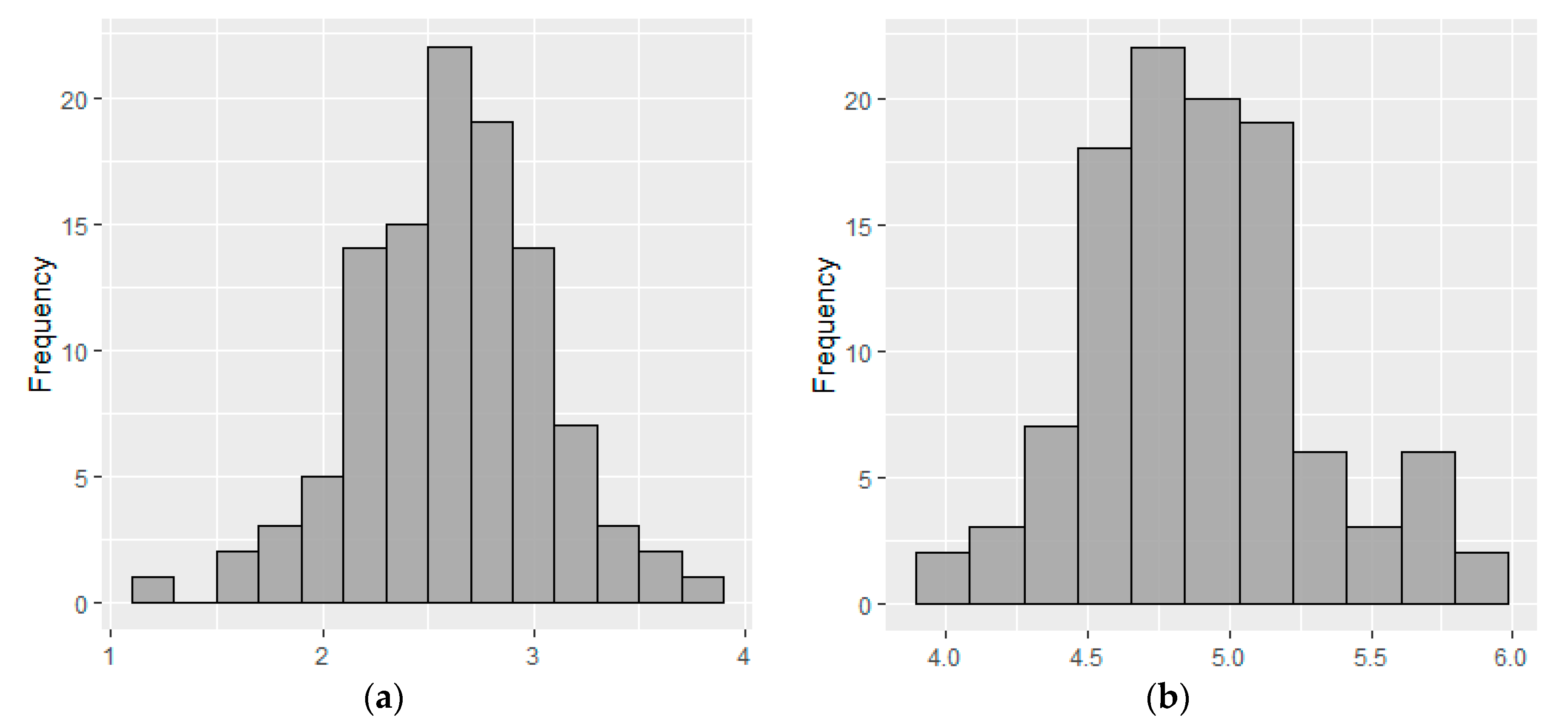
First, the normality of the dependent variables was examined using the Shapiro-Wilk test to verify the goodness of fit [21], obtaining a p-value lower than the stipulated significance level. For this reason, dataset from monthly and per capita water consumption did not come from a normal distribution. Consequently, a logarithmic transformation was employed, the same criterion adopted by Cruz et al. [10]. Then, the normality hypothesis was accepted since the probability value resulting from the test were 0.631 for LNMonthlyConsumption and 0.116 for LNPerCapitaConsumption. Figure 2 displays the histograms for the dependent variables.
In order to assess the dataset, an exploratory analysis was carried out through a source code developed in the software R [22] and RStudio interface. The main attribute values obtained were maximum, minimum, mean, median, and standard deviations as well as tables and graphs (boxplots, histograms, and bar charts).
A correlation analysis was also performed in order to identify numerical association between the two dependent variables and the 57 collected independent variables. The Pearson, Biserial and Spearman’s rank correlation coefficients were calculated for the numerical, dichotomous, and ordinal variables to determine the correlation and significance of each variable, respectively [23,24]. The variables whose p-value was less than 0.1 were considered significant.
3. Results and Discussion
3.1. Water Consumption
It was found that the averages were higher than the medians, when analyzing the descriptive statistics of the dependent variables (Table 1), possibly due to the presence of high consumption values.
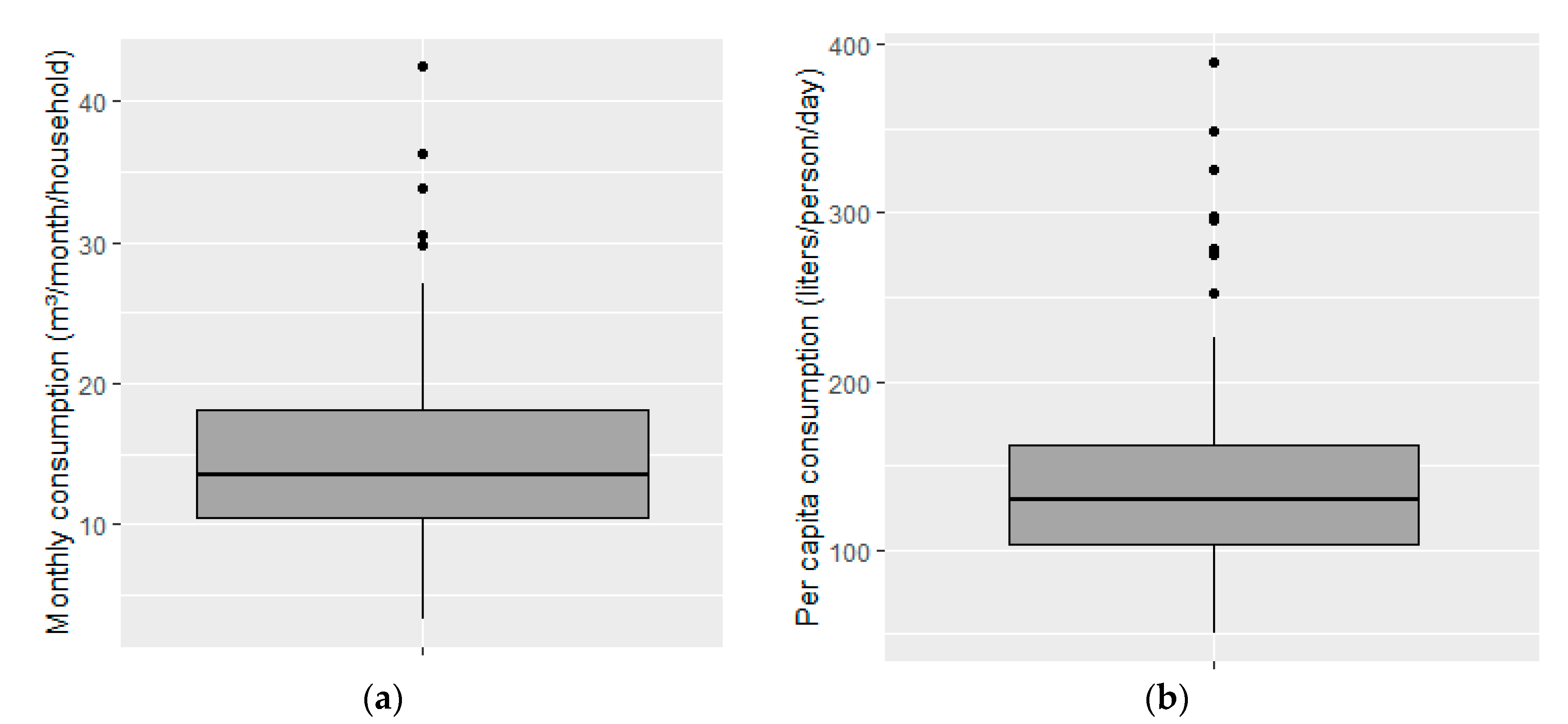
For the monthly water consumption, the observed minimum value was 3.25 m3/month/household and the maximum value was 42.42 m3/month/household, with an average of 15.01 m3/month/household. The boxplot of this variable reveals an asymmetric distribution since approximately 80% of the data are less than 20 m3/month/household (Figure 3a), proving the need for logarithmic transformation.
Per capita consumption ranged from 50.64 liters/person/day to 389.54 liters/person/day, with an average of 144.91 liters/person/day. Figure 3b shows that about 90% of the single-family households consumed less than 225 liters/person/day.
3.2. Correlation Between Variables
The variables that were related to water consumption and per capita consumption were identified through correlation analysis. Table 2 shows the statistically significant variables at 5% and 10% levels (p-value < 0.05 and p-value < 0.10), as well as their correlation coefficient. As in the study by Cruz et al., [10], although most of the coefficients presented low values, with absolute values lower than 0.3 in the scale from zero to one, the correlations were statistically significant. The results indicated that 13 variables were associated with monthly water consumption, while 11 were related to per capita water consumption.
3.3. Surrounding Infrastructure
The surrounding infrastructure refers to the paving of the street and the existence of a public sewage collection system. 76.85% of the 108 households are located in paved streets, but 66.67% are not served by public sewage collection systems. Only 37.35% of the households located in paved streets are served by public sewage collection systems.
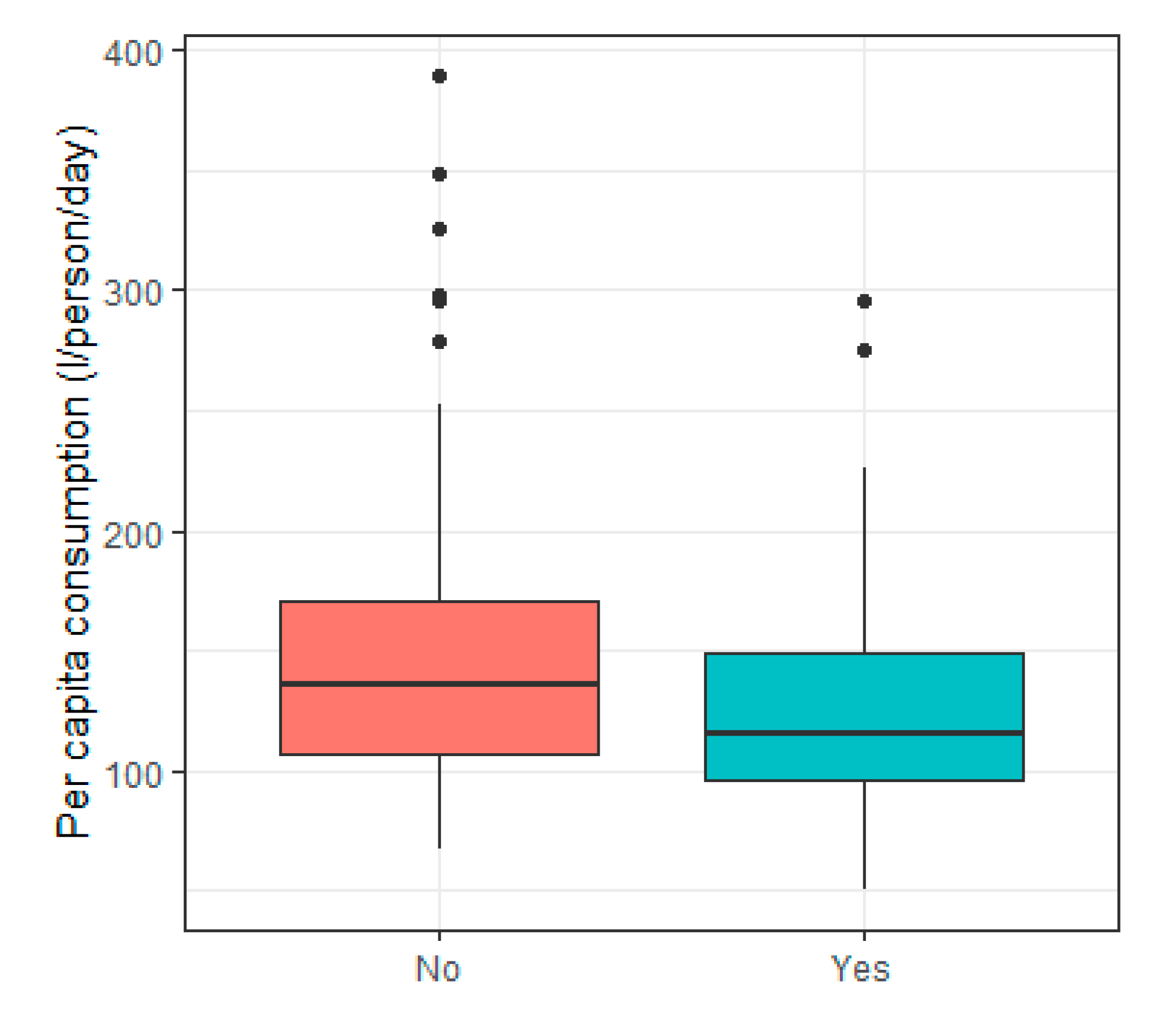
The per capita water consumption displayed a negative correlation (r = −0.278, p < 0.05) with sewage collection, and only this variable was significant, indicating that per capita water consumption decreased by the presence of sewage collection system (Figure 4). This result may be related to the fact that, in Joinville, a rate of 80% is charged on the value of water consumption to cover sewage collection, so the bill is more expensive in households where there is public sewage collection. According to Romano, Salvati, and Guerrini (2014) [26], an applied tariff has a negative effect on residential water consumption, i.e., higher tariffs tend to decrease water consumption, and this is a relevant factor for the management of residential water consumption.
3.4. Socioeconomic and Demographic Characteristics
The socioeconomic and demographic characteristics collected from the households are summarized in Table 3. The average number of residents per household was 3.537 people, with a minimum of one and a maximum of six. In relation to family composition, the average number of women per household was 1.852. Residents under 12 years of age were considered children, those aged 12 to 17 years were considered teenagers, the ones from 18 to 64 years were regarded as adults and those older than 65 as elderly [27,28].
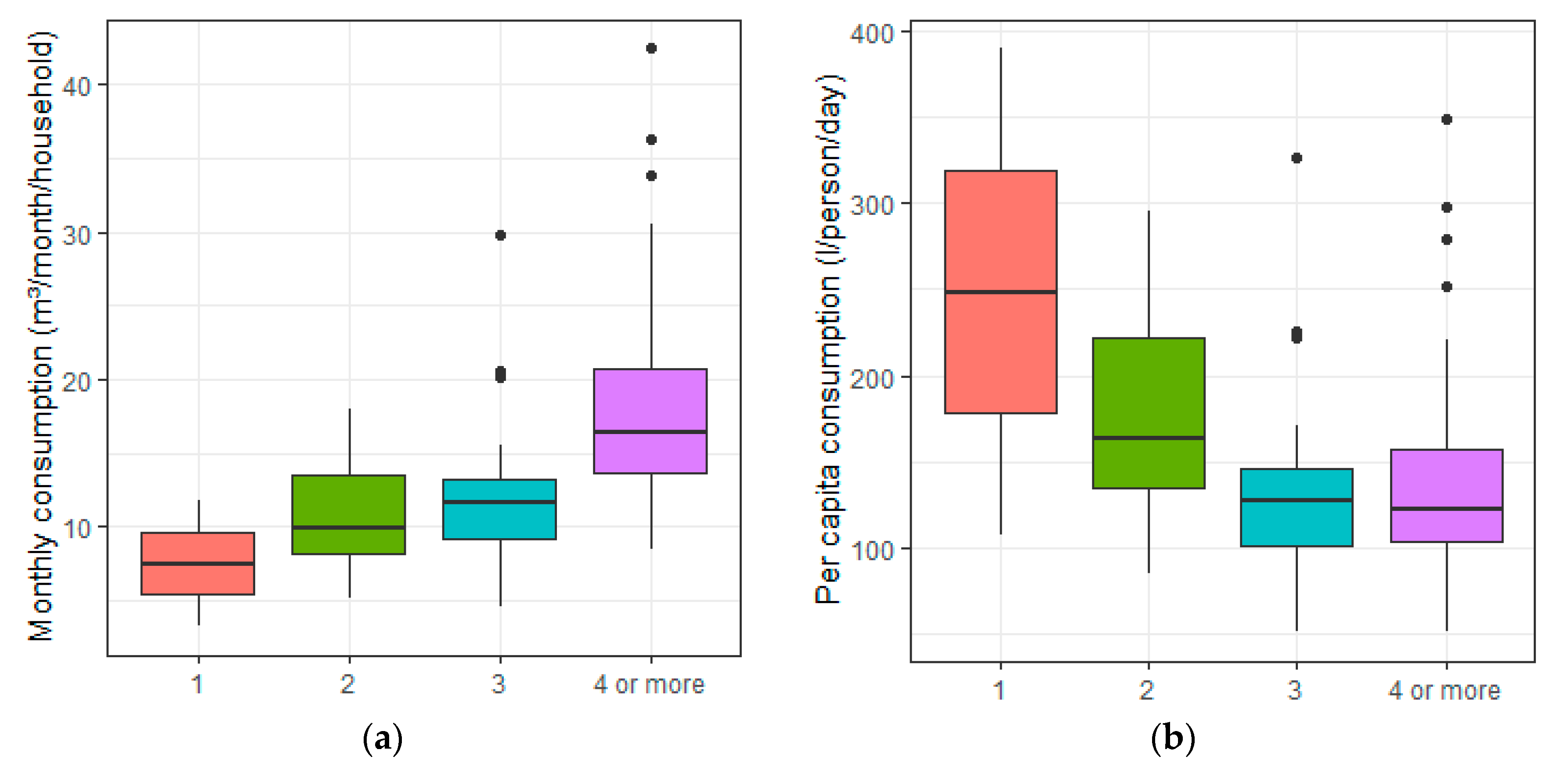
There is a positive and significant relationship between the monthly consumption and the number of residents (r = 0.479, p < 0.05), so the higher the number of residents in the household, the higher the monthly consumption tends to be (Figure 5a). In contrast, the per capita consumption has a negative and significant correlation (r = −0.283, p < 0.05) to the number of residents, so the higher the number of residents in the residence, the lower the per capita water consumption is, as shown in Figure 5b. A study conducted in Iraq by Hussien, Memon, and Savic [7] also showed a decrease in per capita consumption related to the number of residents.
The number of women showed to be significant in both analyses. Monthly water consumption increases based on an increase in the number of women in the residence (r = 0.204, p < 0.05), but per capita water consumption decreases (r = −0.208, p < 0.05), as illustrated in Figure 6. In Mexico, Cruz et al., [10] also identified that consumption increased based on the number of female inhabitants.
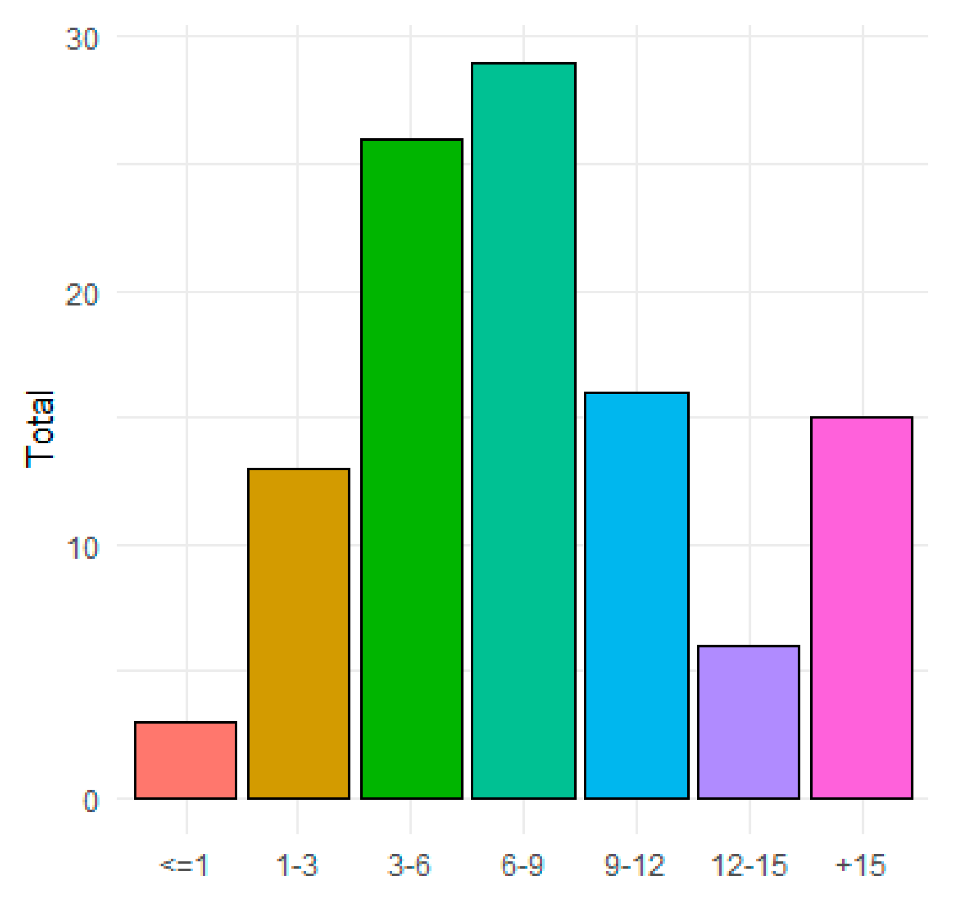
Related to the educational level of the person responsible for the water bill, 26 people have completed an undergraduate degree, 33 have some type of postgraduate degree, 33 have finished high school, and 16 have completed elementary school. The total income per household is concentrated in the ranges between three to 12 minimum wages (the current value in 2018 is R$954.00), as shown in Figure 7. As for the house property, seven are rented and 12 financed, the other 89 are owned and paid off.
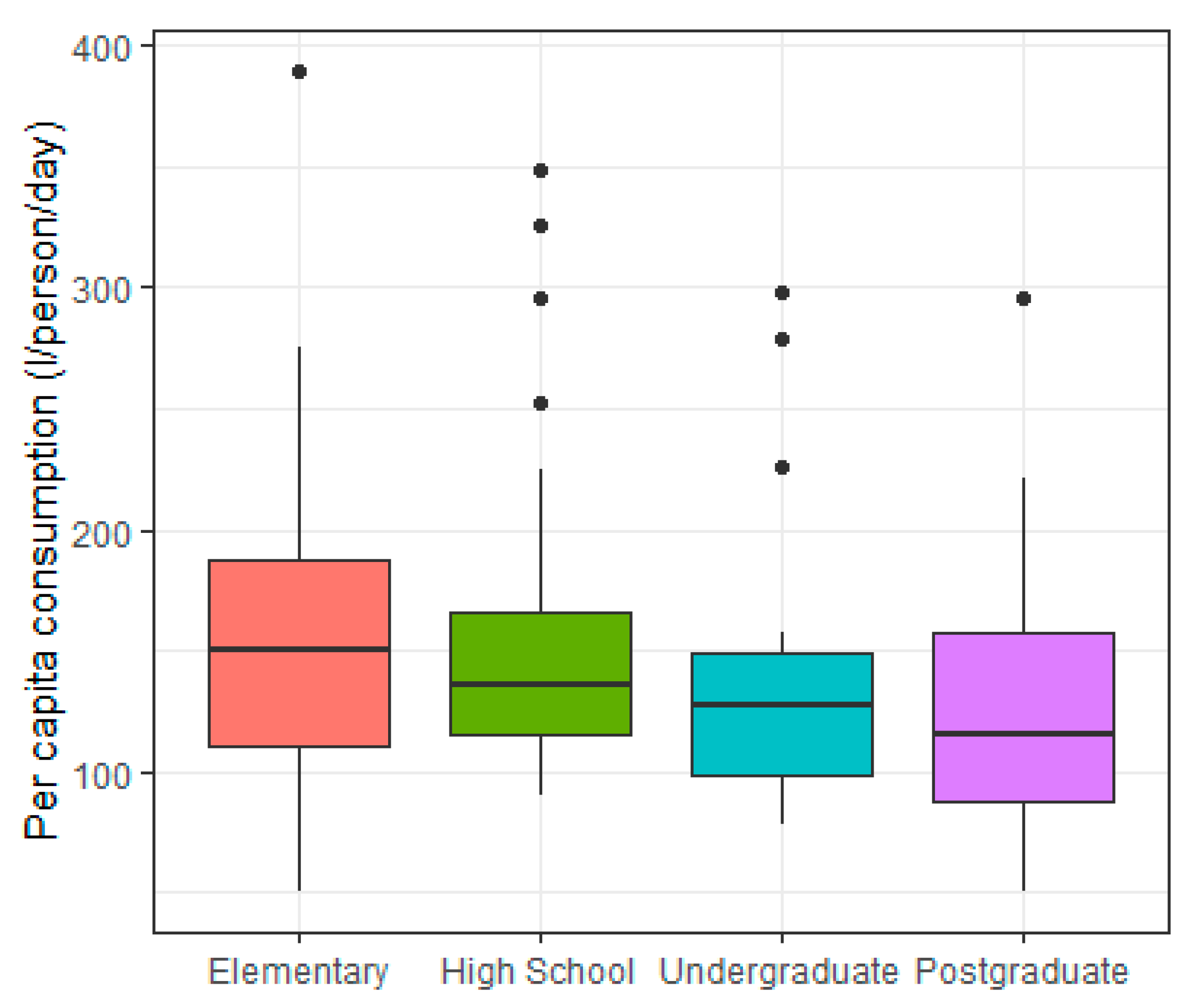
The per capita consumption is significant related to the educational level (r = −0.226, p < 0.05) as shown in Figure 8, indicating that the higher the educational level, the lower the household per capita water consumption is. Pérez-Urdiales and García-Valiñas [29] showed that the education level influences the adoption of technologies that reduce water consumption. The results indicated that families whose head of the household had a higher educational level, the more likely it was to invest in this type of technology.
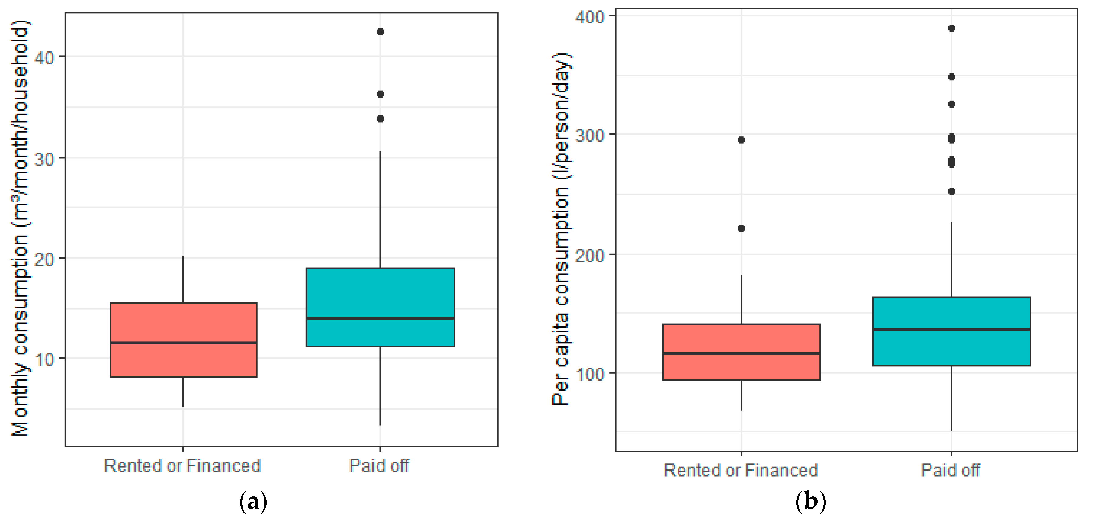
The monthly water consumption (r = −0.342, p < 0.05) and the per capita water consumption (r = −0.233, p < 0.10) tend to decrease when the household is rented or financed (Figure 9). Dias, Kalbusch, and Henning [30] showed that the higher the percentage of tenants in a multifamily building, the lower the consumption was. These results can indicate that those who have expenses with rent and financing tend to save more in water consumption, since in Brazil, expenses such as water and energy bills are the responsibility of the renting resident and not the owner of the residence.
3.5. Constructive Features
There is an average of 3.102 bedrooms in the households, 2.593 bathrooms, and an average of 20.95 years old, three years is the minimum age and 57 years is the maximum age. Monthly water consumption has a positive correlation related to the number of bathrooms (Figure 10) and the p-value indicates that the variable is significant (r = 0.237, p < 0.05). In Madrid, González, Rueda, and Les [31] obtained a similar result, where consumption is influenced by the number of bathrooms, plumbing devices, and number of bedrooms. Cruz et al., [10] also observed that the increase in the number of bathrooms increased the water consumption of Mexican households.
The age of the property was related to monthly water consumption (r = 0.168, p < 0.10), i.e., the older the house is, the higher the monthly water consumption is. A logarithmic transformation (LNAgeProperty) was necessary due to data distribution. In New York’s multi-family buildings, the age of the building also displayed a significant effect on the intensity of water use [12].
On average the property land area is 499.78 m2 and the average total built area per household is 165.6 m2. The monthly consumption of the household (r = 0.288, p < 0.05) and per capita consumption (r = 0.184, p < 0.10) increase based on the increase of the total built area. Mayer and DeOreo [32] also achieved a relationship between increased water consumption in households with larger built area in the USA, while Loh and Coghlan [33] found a decrease in consumption related to the size of the household in Australia.
One-story houses represented 57.4% of the sample, 32.4% are two-story houses and 10.2% are row houses. 15.7% of the households have swimming pool and 93.5% have reservoir. The monthly water consumption and per capita water consumption decrease based on the presence of reservoir, as it is significant for per capita consumption (r = −0.346, p < 0.05) (Figure 11).
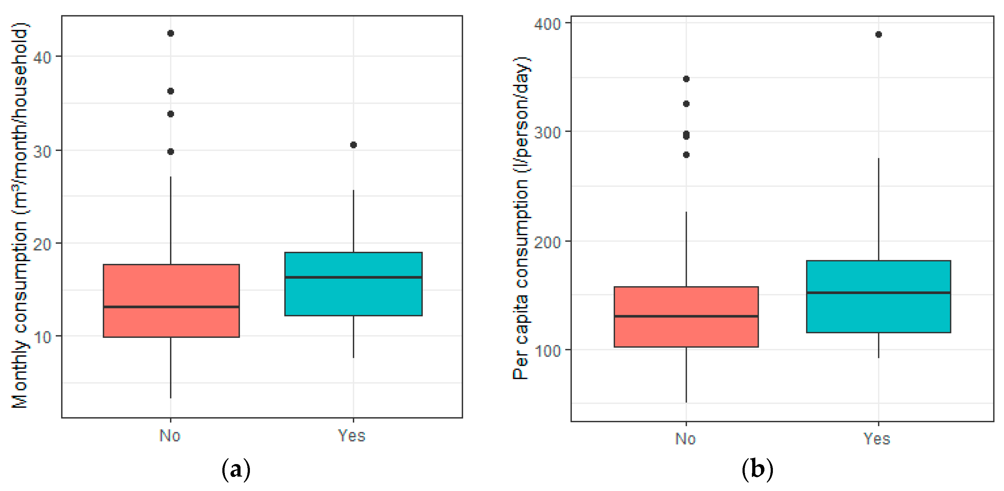
Water shortages are not usual in 79.6% of households. The frequency was also analyzed, indicating that water shortages occur monthly in 17.6% of the households and weekly in 1.9% of cases. Water shortages were significant in monthly water consumption (r = 0.225, p < 0.10) and for the per capita consumption (r = 0.254, p < 0.05) as shown in Figure 12.
There is a bathtub in 15.7% of households, but 64.7% of the residents declared that they do not use this plumbing device. Moreover, it was intended to analyze the existence of alternative water systems (rainwater harvesting system, underground water intake, water reuse system), but only four houses had some of these systems. In one of the households there is a rainwater harvesting system, one household has underground intake (water well), and in two houses there is water reuse system. Water from the alternative system is used for washing external areas of the house in these households, but there is no meter for that system in any of them.
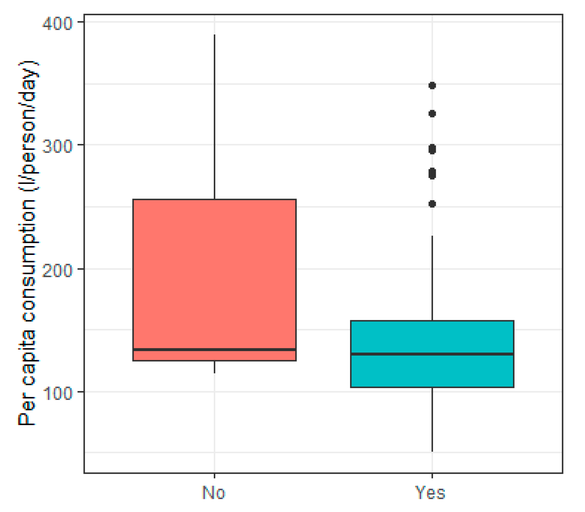
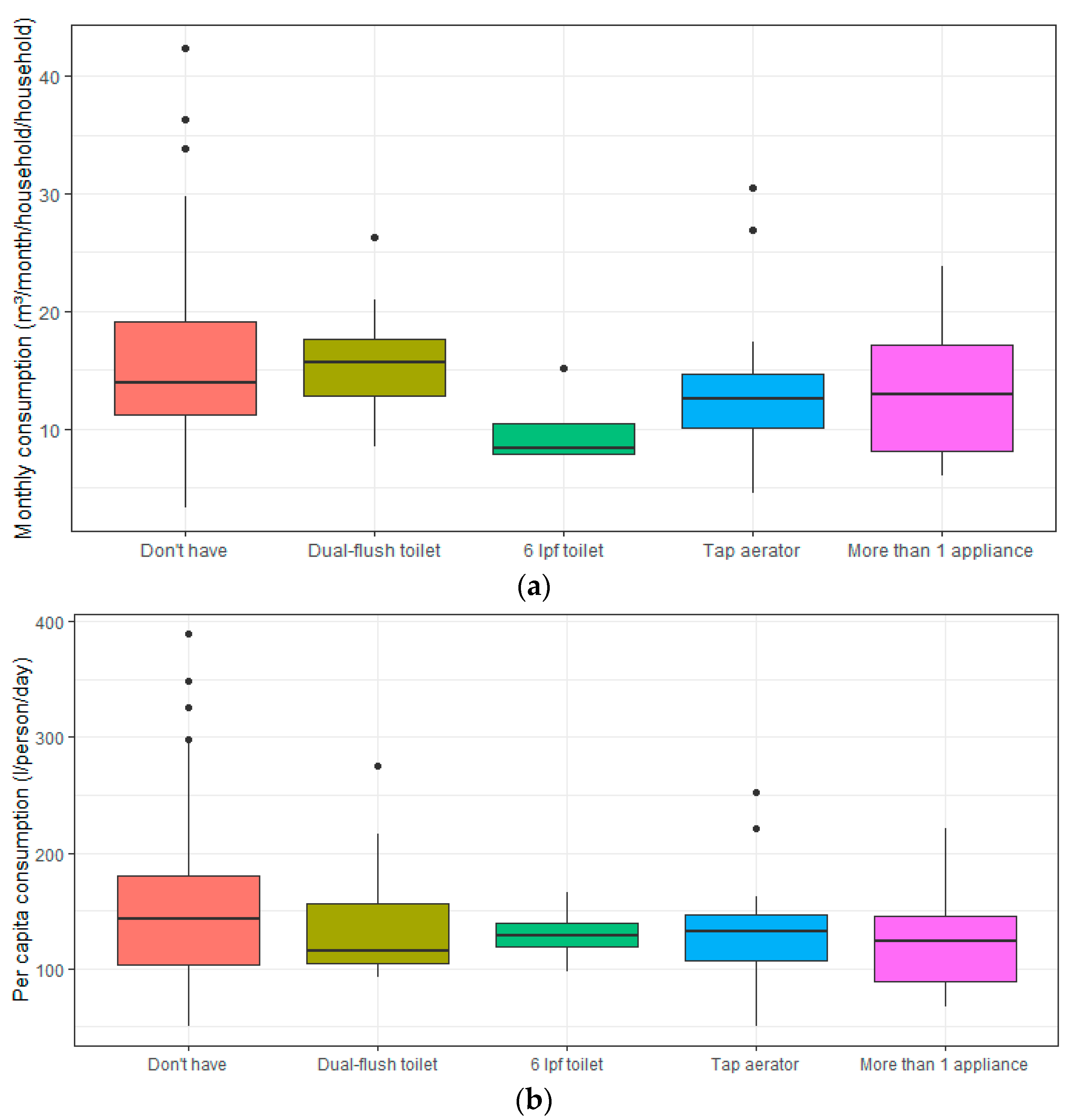
3.6. Installed Fixtures
A total of 42.59% houses have installed water-saving fixtures. 22.22% have dual-flush toilets, 11.11% have 6 liters per flush toilet, 26.85% have tap aerators, and 13.89% have more than one appliance installed. Among the strategies for reducing consumption (rainwater harvesting system, greywater reuse system, and water-efficient appliances), the use of water-saving devices provides one of the greatest environmental benefit due to lower embodied energy throughout their life cycle [3]. Analyzing the devices separately, the presence of tap aerators showed to be significant for decreasing the monthly water consumption (r = −0.237, p < 0.10) and the per capita water consumption (r = −0.226, p < 0.10) as shown in Figure 13. The presence of 6 liters per flush (lpf) toilet also decreases monthly water consumption (r = −0.251, p < 0.10). This information can be helpful when planning incentive policies for the acquisition of water-saving devices since they contribute significantly to decreased consumption. Seattle legislation, for example, has already incorporated several programs focused on water efficiency such as the use of more efficient appliances in the kitchen, bathroom, and irrigation, which could serve as a model for Brazilian cities [34].
3.7. Water-Use Habits
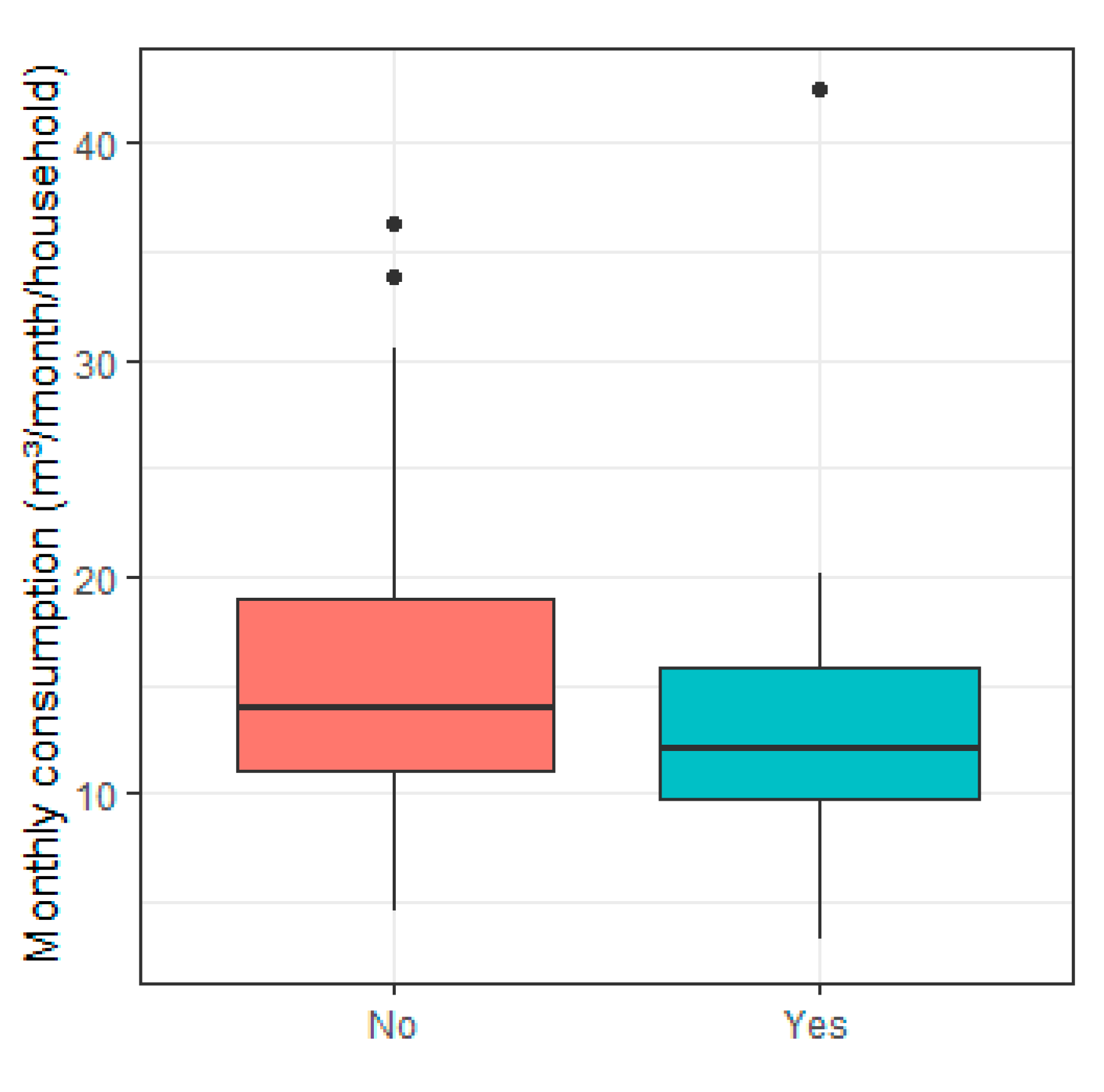
The evaluated water-use habits were the purchase of purified bottled drinking water, reusing washing machine water, car washing, outdoor areas washing, and garden irrigation. Thirty-point-fifty-six percent buy purified bottled drinking water. As for the washing machine water, 24.08% have the habit of reusing, 15.74% use for washing outdoor areas, 2.78% washing other clothes, 1.85% use for flushing the toilet, 2.78% use for cleaning the house and 0.93% use for watering the garden. The reuse of the washing machine water is significant for decreasing monthly water consumption (r = −0.239, p < 0.10) (Figure 14).
70.37% of the respondents wash the car at home (19.44% use bucket, 12.04% use hose, 15.74% use high-pressure washer). The use of high-pressure washer is significant to increasing monthly water consumption (r = 0.258, p < 0.05) (Figure 15). 23.15% use more than one kind of equipment to wash the car at home. 12.04% wash the car weekly, 24.07% twice monthly, and 35.19% monthly.
As for the habit of washing outdoor areas, 67.59% wash household outdoor areas (13.89% use bucket, 12.04% use hose and 32.41% use high-pressure washer and 9.26% use more than one kind of equipment). The use of high-pressure washer for washing outdoor areas is significant to increasing monthly water consumption (r = 0.318, p < 0.05) (Figure 16).
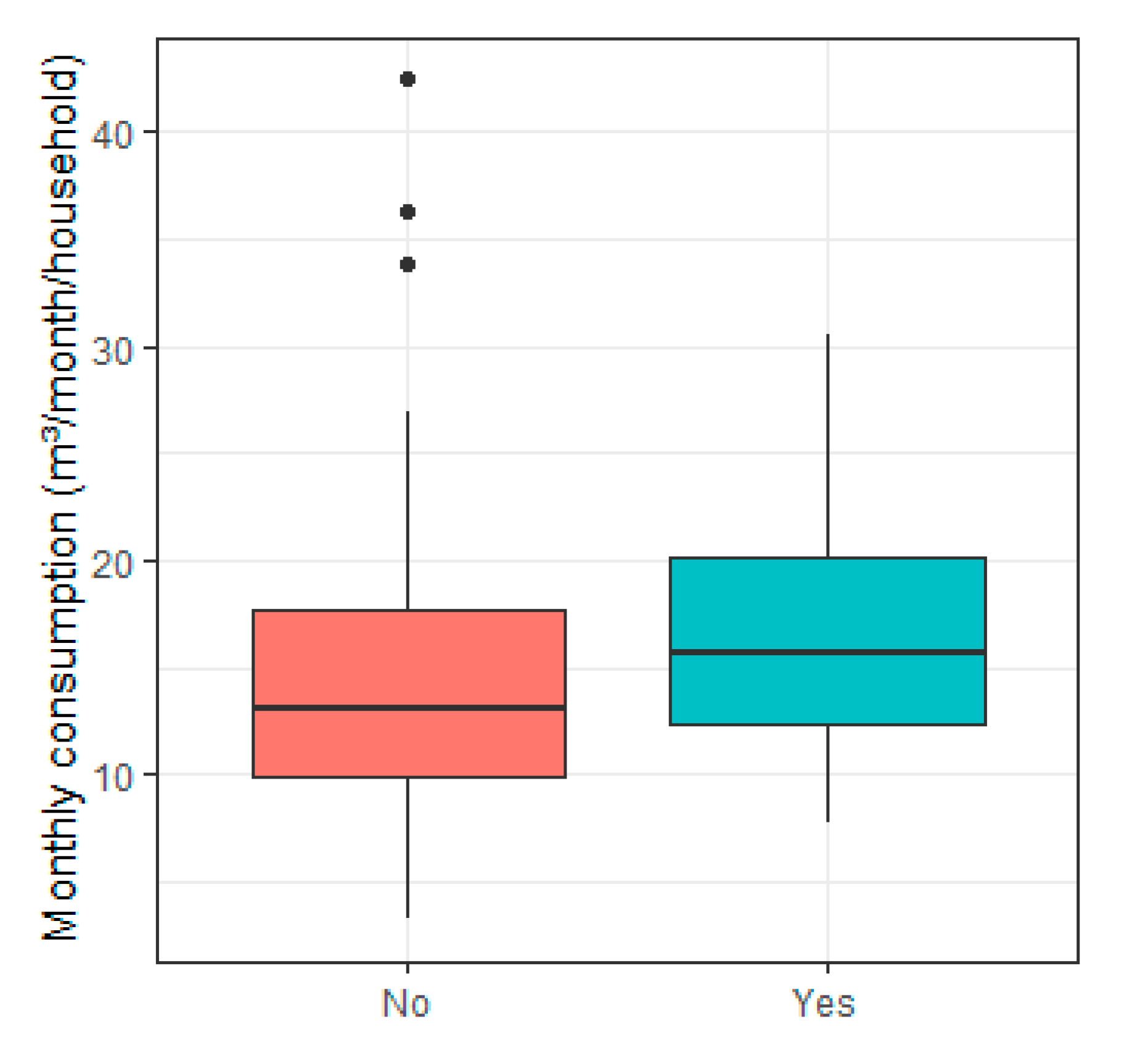
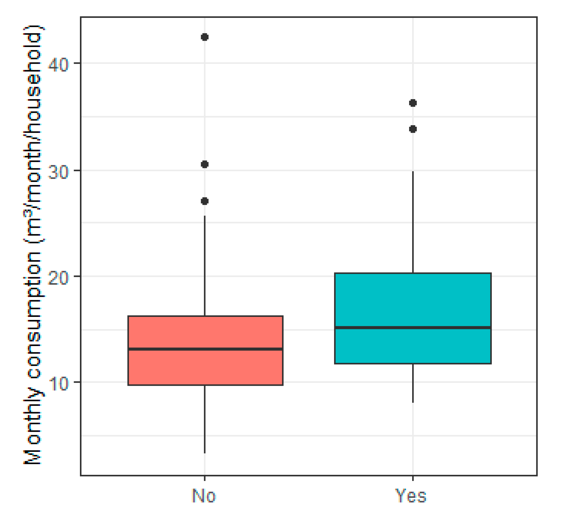
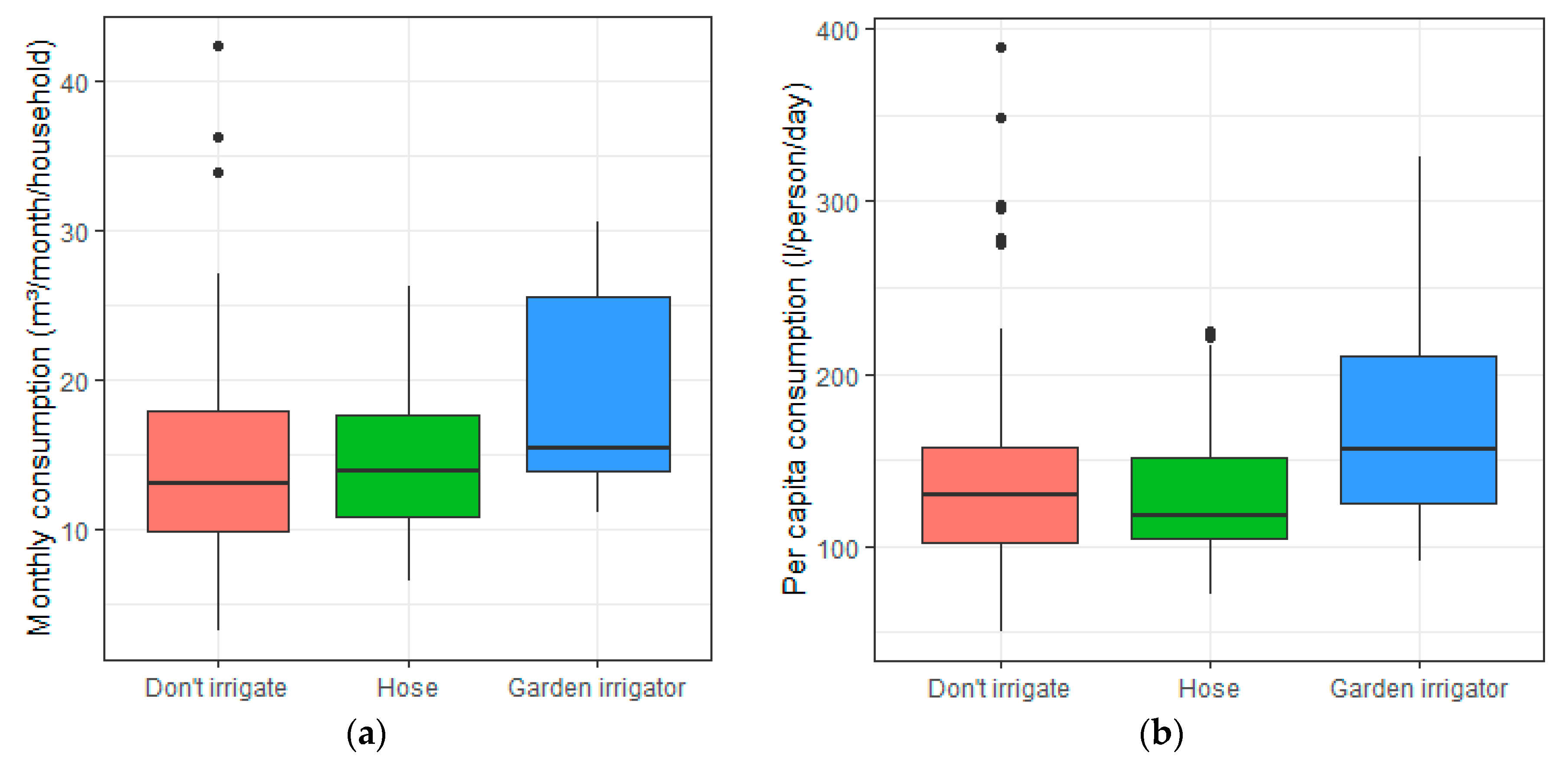
Regarding garden irrigation, 25% of the respondents irrigate the garden (16.7% use hose and 8.3% use irrigator), and the use of irrigators is significant in monthly water consumption (r = 0.382, p < 0.05) and in per capita consumption (r = 0.288, p < 0.10) (Figure 17). Regarding irrigation frequency, 18.5% of those who irrigate the garden, irrigate it daily, 66.7% irrigate it weekly, and 14.8% irrigate it monthly. In the study conducted by Domene et al., [35], the water consumed annually in the garden reached 30% of the total water consumed in the household and 50% during the summer season.
Koop et al., [36] present a literature review on users behavior influence on domestic water consumption. The authors focused specifically on behavior influencing as a way to promote domestic water saving. Most of the 52 analyzed studies were conducted in developed countries with water stress. The authors state that domestic water savings can be achieved through economic incentives, technical improvements or policy instruments and regulations.
Water demand management policies have been employed in recent decades as an important strategy to reduce water consumption in cities [37]. Obtaining information about the factors that influence water consumption is essential to ensure that public policies to reduce consumption are correctly oriented.
As a suggestion for the development of future works, the investigation of the influence of the presence of domestic animals and the type of water heating system can be cited. In Brazil, the use of electric showers is predominant, mainly due to the low initial cost and the ease of installation and operation [38]. Some studies indicate that 83.6% of Brazilian households with water heating system use electricity (predominantly with electric showerheads) and that this average coverage is especially significant in the most populous and cold regions of Southern Brazil [38,39].
4. Conclusions
This study presented an exploratory analysis of factors that may influence water consumption in households in Joinville, Southern Brazil. The surrounding infrastructure, socioeconomic and demographic characteristics, constructive features, installed plumbing fixtures and consumption habits were considered. The correlation of 57 independent variables with monthly consumption and per capita consumption was investigated.
The variables that proved to be significant for increasing monthly water consumption in this study (p-value < 0.05 and p-value < 0.10) were the number of residents, number of women, household situation, number of bathrooms, age of the property, total built area, water shortage, use of irrigators in the garden, use of high-pressure washer for washing the car and outdoor areas. Furthermore, variables such as the presence of aerator on taps, 6 lpf toilets, and reusing water from the washing machine reduced the monthly consumption.
The significant variables for per capita water consumption were the presence of public sewage collection system, number of residents, number of women, educational level, house property (rented or financed), total built area, presence of reservoir, water shortage, the presence of water-saving fixtures, and use of irrigators in the garden. Water shortage, household ownership, built area, and use of irrigator increased the per capita consumption while the other mentioned variables caused a decrease in per capita water consumption.
This study presented variables that influence water consumption in the city of Joinville, Southern Brazil. These results will be used for multiple linear regression analysis and verification of spatial variations in water consumption, proceeding the development of the research. Ultimately, the present study represents an initial step in the evaluation of water consumption in single-family households in Joinville and can contribute to the development of public policies linked to sustainability and population awareness related to domestic water use.
The results presented may guide the creation of public incentives to ensure that the population has access to water reservoirs, which is predicted in the Brazilian technical standards. Similarly, there may be incentives for the purchase of water saving plumbing fixtures or campaigns to promote water saving habits.
Author Contributions
Conceptualization, J.G., A.K. and E.H.; Methodology, J.G., A.K. and E.H.; Software, J.G. and L.S.; Formal analysis, J.G., L.S., A.K. and E.H.; Writing—original draft preparation, J.G. and L.S.; Writing—review and editing, A.K. and E.H.; Supervision, A.K. and E.H.
Funding
This research was supported by the Conselho Nacional de Desenvolvimento Científico e Tecnológico—CNPq and Fundação de Amparo à Pesquisa e Inovação do Estado de Santa Catarina—FAPESC (grant number 2017 TR789).
Acknowledgments
The authors would like to thank Companhia Águas de Joinville for data provision.
Conflicts of Interest
The authors declare no conflict of interest.
References
- Adapa, S. Factors influencing consumption and anti-consumption of recycled water: Evidence from Australia. J. Clean. Prod. 2018, 201, 624–635. [Google Scholar] [CrossRef]
- UN OCHA. Water Scarcity and Humanitarian Action: Key Emerging Trends and Challenges Brief; Policy Development and Studies Branch: Geneva, Switzerland, 2010; Available online: https://www.unocha.org/es/publication/policy-briefs-studies/water-scarcity-and-humanitarian-action-key-emerging-trends-and (accessed on 2 June 2019).
- Marinoski, A.K.; Rupp, R.F.; Ghisi, E. Environmental benefit analysis of strategies for potable water savings in residential buildings. J. Environ. Manag. 2018, 206, 28–39. [Google Scholar] [CrossRef] [PubMed]
- Willis, R.M.; Stewart, R.A.; Giurco, D.P.; Talebpour, M.R.; Mousavinejad, A. End use water consumption in households: Impact of socio-demographic factors and efficient devices. J. Clean. Prod. 2013, 60, 107–115. [Google Scholar] [CrossRef]
- Willis, R.M.; Stewart, R.A.; Panuwatwanich, K.; Williams, P.R.; Hollingsworth, A.L. Quantifying the influence of environmental and water conservation attitudes on household end use water consumption. J. Environ. Manag. 2011, 92, 1996–2009. [Google Scholar] [CrossRef] [PubMed] [Green Version]
- Nauges, C.; Whittington, D. Estimation of water demand in developing countries: An overview. World Bank Res. Obs. 2009, 25, 263–294. [Google Scholar] [CrossRef]
- Hussien, W.A.; Memon, F.A.; Savic, D.A. Assessing and Modelling the Influence of Household Characteristics on Per Capita Water Consumption. Water Resour. Manag. 2016, 30, 2931–2955. [Google Scholar] [CrossRef] [Green Version]
- Fan, L.; Gai, L.; Tong, Y.; Li, R. Urban water consumption and its influencing factors in China: Evidence from 286 cities. J. Clean. Prod. 2017, 166, 124–133. [Google Scholar] [CrossRef]
- Sant’Ana, D.; Mazzega, P. Socioeconomic analysis of domestic water end-use consumption in the Federal District, Brazil. Sustain. Water Resour. Manag. 2018, 4, 921–936. [Google Scholar] [CrossRef]
- De la Cruz, A.O.; Alvarez-Chavez, C.R.; Ramos-Corella, M.A.; Soto-Hernandez, F. Determinants of domestic water consumption in Hermosillo, Sonora, Mexico. J. Clean. Prod. 2017, 142, 1901–1910. [Google Scholar] [CrossRef]
- Domene, E.; Saurí, D. Urbanisation and water consumption: Influencing factors in the metropolitan region of Barcelona. Urban Stud. 2006, 43, 1605–1623. [Google Scholar] [CrossRef]
- Kontokosta, C.E.; Jain, R.K. Modeling the determinants of large-scale building water use: Implications for data-driven urban sustainability policy. Sustain. Cities Soc. 2015, 18, 44–55. [Google Scholar] [CrossRef] [Green Version]
- Romano, G.; Salvati, N.; Guerrini, A. An empirical analysis of the determinants of water demand in Italy. J. Clean. Prod. 2016, 130, 74–81. [Google Scholar] [CrossRef]
- Dos Santos, S.M.; Farias, M.M.M.W.E.C. Potential for rainwater harvesting in a dry climate: Assessments in a semiarid region in northeast Brazil. J. Clean. Prod. 2017, 164, 1007–1015. [Google Scholar] [CrossRef]
- IPPUJ. Joinville Cidade em Dados 2018—Ambiente Construído. 2018. Available online: https://www.joinville.sc.gov.br/publicacoes/joinville-cidade-em-dados-2018/ (accessed on 21 January 2019).
- IBGE. Instituto Brasileiro de Geografia e Estatística. 2018. Available online: https://cidades.ibge.gov.br/brasil/sc/joinville/panorama (accessed on 21 January 2019).
- IBGE. Instituto Brasileiro de Geografia e Estatística. 2010. Available online: https://cidades.ibge.gov.br/brasil/sc/joinville/panorama (accessed on 24 January 2019).
- SANTA CATARINA. Secretaria de Estado da Fazenda. 2012. Available online: http://www.sef.sc.gov.br/ (accessed on 24 January 2019).
- Galloway, A. Non-Probability Sampling. Encycl. Soc. Meas. 2005, 2, 859–864. [Google Scholar]
- Cohen, J. A Power Primer. Psychol. Bull. 1992, 112, 155–159. [Google Scholar] [CrossRef]
- Tufféry, S. Data Mining and Statistics for Decision Making; Wiley & Sons: Chichester, UK, 2011. [Google Scholar]
- R CORE TEAM. R: A language and Environment for Statistical Computing and Graphics; Version 3.4.3; The R Foundation: Auckland, New Zealand, 2019; Available online: https://www.r-project.org/ (accessed on 18 June 2019).
- Lewis-Beck, M.S.; Bryman, A.; Liao, T.F. The SAGE Encyclopedia of Social Science Research Methods, 3rd ed.; SAGE Publications: Thousand Oaks, CA, USA, 2004. [Google Scholar] [CrossRef]
- Saldink, N.J. Encyclopedia of Measurement and Statistics, 3rd ed.; SAGE Publications: Thousand Oaks, CA, USA, 2007. [Google Scholar]
- Ghisi, E.; Oliveira, S.M. Potential for potable water savings by combining the use of rainwater and greywater in houses in southern Brazil. Build. Environ. 2007, 42, 1731–1742. [Google Scholar] [CrossRef]
- Romano, G.; Salvati, N.; Guerrini, A. Estimating the determinants of residential water demand in Italy. Water 2014, 5, 2929–2945. [Google Scholar] [CrossRef]
- BRASIL. Lei n. 8.069 de 13 de Julho de 1990. Dispõe Sobre o Estatuto da Criança e do Adolescente e dá Outras Providências. Available online: http://www.planalto.gov.br/ccivil_03/leis/l8069.htm (accessed on 21 June 2019).
- BRASIL. Lei n. 10.741 de 1 de Outubro de 2003. Dispõe Sobre o Estatuto do Idoso e dá Outras Providências. Available online: http://www.planalto.gov.br/ccivil_03/leis/2003/l10.741.htm (accessed on 21 June 2019).
- Pérez-Urdiales, M.; García-Valiñas, M.Á. Efficient water-using technologies and habits: A disaggregated analysis in the water sector. Ecol. Econ. 2016, 128, 117–129. [Google Scholar] [CrossRef]
- Dias, T.F.; Kalbusch, A.; Henning, E. Factors influencing water consumption in buildings in southern Brazil. J. Clean. Prod. 2018, 184, 160–167. [Google Scholar] [CrossRef]
- González, F.C.; Rueda, T.M.; Les, S.O. Cuadernos de I+D+I 4: Microcomponentes y Factores Explicativos del Consumo Doméstico de Agua en la Comunidad de Madrid. Canal de Isabel II. Available online: http://www.madrid.org/bvirtual/BVCM008675.pdf (accessed on 6 June 2019).
- Mayer, P.W.; DeOreo, W.B. Residential End Uses of Water; AWWARF: Denver, CO, USA, 1999. [Google Scholar]
- Loh, M.; Coghlan, P. Domestic Water Use Study; Water Corporation: Perth, Australia, 2003. [Google Scholar]
- Ribeiro, J.M.P.; Bocasanta, S.L.; Ávila, B.O.; Magtoto, M.; Jonck, A.V.; Gabriel, G.M.; De Andrade Guerra, J.B.S.O. The adoption of strategies for sustainable cities: A comparative study between Seattle and Florianopolis legislation for energy and water efficiency in buildings. J. Clean. Prod. 2018, 197, 366–378. [Google Scholar] [CrossRef]
- Domene, E.; Saurí, D.; Parés, M. Urbanization and Sustainable Resource Use: The Case of Garden Watering in the Metropolitan Region of Barcelona. Urban Geogr. 2005, 26, 520–535. [Google Scholar] [CrossRef]
- Koop, S.H.A.; Van Dorssen, A.J.; Brouwer, S. Enhancing domestic water conservation behavior: A review of empirical studies on influencing tatics. J. Environ. Manag. 2019, 247, 867–876. [Google Scholar] [CrossRef]
- Stavenhagen, M.; Buurman, J.; Tortajada, C. Saving water in cities: Assessing policies for residential water demand management in four cities in Europe. Cities 2018, 79, 187–195. [Google Scholar] [CrossRef]
- Cruz, T.; Schaeffer, R.; Lucena, A.F.P.; Melo, S.; Dutra, R. Solar water heating technical economic potential in the household sector in Brazil. Renew. Energy 2019, 146, 1618–1639. [Google Scholar] [CrossRef]
- Cardemil, J.M.; Starke, A.R.; Colle, S. Multi-objective optimization for reducing the auxiliary electric energy peak in low cost solar domestic hot-water heating systems in Brazil. Sol. Energy 2018, 163, 486–496. [Google Scholar] [CrossRef]
Figure 1.
Location of participating houses in the urban area of Joinville.

Figure 2.
Histogram: (a) LNMonthlyConsumption; (b) LNPerCapitaConsumption.

Figure 3.
(a) Boxplot of the monthly water consumption (m3/month); (b) boxplot of the per capita water consumption (liters/person/day).
Figure 3.
(a) Boxplot of the monthly water consumption (m3/month); (b) boxplot of the per capita water consumption (liters/person/day).

Figure 4.
Per capita water consumption related to the sewage collection system.

Figure 5.
(a) Monthly water consumption related to the number of residents; (b) per capita water consumption related to the number of residents.
Figure 5.
(a) Monthly water consumption related to the number of residents; (b) per capita water consumption related to the number of residents.

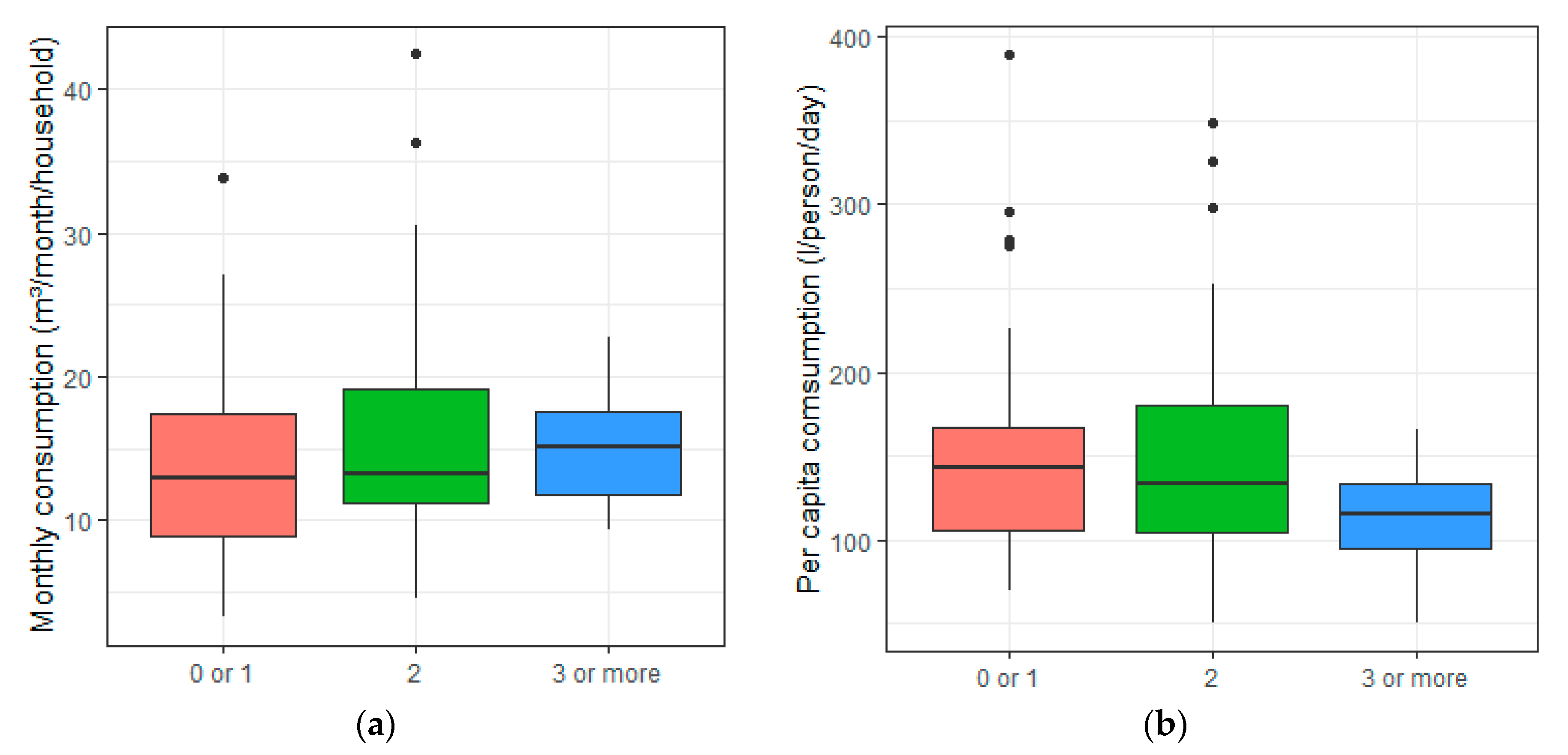
Figure 6.
(a) Monthly water consumption related to the number of women; (b) per capita water consumption related to the number of women.
Figure 6.
(a) Monthly water consumption related to the number of women; (b) per capita water consumption related to the number of women.

Figure 7.
Monthly income per household.

Figure 8.
Per capita water consumption related to educational level.

Figure 9.
(a) Monthly water consumption related to the house property; (b) per capita water consumption related to the house property.
Figure 9.
(a) Monthly water consumption related to the house property; (b) per capita water consumption related to the house property.

Figure 10.
Monthly water consumption related to the number of bathrooms.

Figure 11.
Relationship between reservoir and per capita consumption.

Figure 12.
(a) Relationship between water shortage and monthly water consumption; (b) Relationship between water shortage and per capita water consumption.
Figure 12.
(a) Relationship between water shortage and monthly water consumption; (b) Relationship between water shortage and per capita water consumption.

Figure 13.
(a) Relationship between monthly water consumption and water-efficient appliances; (b) Relationship between per capita water consumption and water-efficient appliances.
Figure 13.
(a) Relationship between monthly water consumption and water-efficient appliances; (b) Relationship between per capita water consumption and water-efficient appliances.

Figure 14.
Relationship between monthly water consumption and reuse of the washing machine water.

Figure 15.
Relationship between monthly consumption and the use of high-pressure washer for car washing.
Figure 15.
Relationship between monthly consumption and the use of high-pressure washer for car washing.

Figure 16.
Relationship between monthly water consumption and using of high-pressure washer for washing outdoor areas.
Figure 16.
Relationship between monthly water consumption and using of high-pressure washer for washing outdoor areas.

Figure 17.
(a) Relationship between monthly water consumption and garden irrigation; (b) Relationship between per capita water consumption and garden irrigation.
Figure 17.
(a) Relationship between monthly water consumption and garden irrigation; (b) Relationship between per capita water consumption and garden irrigation.


Table 1.
Descriptive statistics of the variables monthly water consumption and per capita water consumption.
Table 1.
Descriptive statistics of the variables monthly water consumption and per capita water consumption.
| Variable | Minimum | 1st Quartile | Median | Mean | 3rd Quartile | Maximum | Standard Deviation |
|---|---|---|---|---|---|---|---|
| Monthly water consumption (m3/month/household) | 3.25 | 10.46 | 13.56 | 15.01 | 18.12 | 42.42 | 6.669 |
| Per capita water consumption (liters/person/day) | 50.64 | 103.68 | 130.36 | 144.91 | 162.06 | 389.54 | 63.370 |
Table 2.
Independent variables correlated to monthly water consumption and per capita water consumption.
Table 2.
Independent variables correlated to monthly water consumption and per capita water consumption.
| N | Description | LN Monthly Water Consumption | LN Per Capita Water Consumption |
|---|---|---|---|
| Coefficient | |||
| Surrounding infrastructure | |||
| 1 | Existence of public sewage collection system | - | −0.278 a |
| Socioeconomic and demographic characteristics | |||
| 2 | Total number of residents | 0.479 a | −0.283 a |
| 3 | Number of women | 0.204 a | −0.208 a |
| 4 | Educational level of the person responsible for the water bill | - | −0.226 a |
| 5 | House property (rented or financed) | −0.342 a | −0.233 b |
| Constructive features | |||
| 6 | Number of bathrooms | 0.237 a | - |
| 7 | Logarithm of building age (years) | 0.168 b | - |
| 8 | Built area (m2)—includes house area, garage, and shed | 0.288 a | 0.184 b |
| 9 | Presence of reservoir | - | −0.346 a |
| 10 | Water shortage in the household | 0.225 b | 0.254 a |
| Installed fixtures | |||
| 11 | Presence of water-efficient appliances (dual-flush toilets, 6 liters per flush toilet or tap aerators) | - | −0.217 b |
| 12 | Presence of aerators | −0.237 b | −0.226 b |
| 13 | Presence of 6 liters per flush toilets | −0.251 b | - |
| Consumption habits | |||
| 14 | Water reuse from washing machine | −0.239 b | - |
| 15 | Use of high-pressure washer for washing the car | 0.258 a | - |
| 16 | Use of high-pressure washer for washing outdoor areas | 0.318 a | - |
| 17 | Use of irrigator for garden watering | 0.382 a | 0.288 b |
a The correlation is significant at the level of 0.05. b The correlation is significant at the level of 0.10.
Table 3.
Demographic characteristics.
| Characteristics | min | Median | Mean | Max | sd |
|---|---|---|---|---|---|
| # of residents | 1 | 4 | 3.537 | 6 | 1.018 |
| # of women | 0 | 2 | 1.852 | 4 | 0.783 |
| # of children | 0 | 0 | 0.315 | 3 | 0.651 |
| # of teenagers | 0 | 0 | 0.231 | 2 | 0.466 |
| # of adults | 1 | 3 | 2.833 | 5 | 0.881 |
| # of elderly | 0 | 0 | 0.130 | 2 | 0.364 |
© 2019 by the authors. Licensee MDPI, Basel, Switzerland. This article is an open access article distributed under the terms and conditions of the Creative Commons Attribution (CC BY) license (http://creativecommons.org/licenses/by/4.0/).
Share and Cite
MDPI and ACS Style
Garcia, J.; Salfer, L.R.; Kalbusch, A.; Henning, E. Identifying the Drivers of Water Consumption in Single-Family Households in Joinville, Southern Brazil. Water 2019, 11, 1990. https://doi.org/10.3390/w11101990
AMA Style
Garcia J, Salfer LR, Kalbusch A, Henning E. Identifying the Drivers of Water Consumption in Single-Family Households in Joinville, Southern Brazil. Water. 2019; 11(10):1990. https://doi.org/10.3390/w11101990
Chicago/Turabian StyleGarcia, Janine, Luis Ricardo Salfer, Andreza Kalbusch, and Elisa Henning. 2019. "Identifying the Drivers of Water Consumption in Single-Family Households in Joinville, Southern Brazil" Water 11, no. 10: 1990. https://doi.org/10.3390/w11101990
Note that from the first issue of 2016, this journal uses article numbers instead of page numbers. See further details here.