Sediment Transport Mechanisms in a Lagoon with High River Discharge and Sediment Loading
by
 , , ,
, , ,
Jovita Mėžinė
1,*, 
Christian Ferrarin
2,
Diana Vaičiūtė
1,
Rasa Idzelytė
1,
Petras Zemlys
1 and
Georg Umgiesser
1,2 1
Marine Research Institute, Klaipėda University, Universiteto alley 17, 92294 Klaipėda, Lithuania
2
CNR—National Research Council of Italy, ISMAR—Institute of Marine Sciences, Venice, Castello 2737/f, 30122 Venice, Italy
*
Author to whom correspondence should be addressed.
Water 2019, 11(10), 1970; https://doi.org/10.3390/w11101970
Submission received: 21 August 2019
/
Revised: 14 September 2019
/
Accepted: 17 September 2019
/
Published: 21 September 2019
(This article belongs to the Special Issue Study of Lagoons and Other Shallow Water Bodies Through the Application of Numerical Models)
Abstract
:The aim of this study was to investigate the sediment dynamics in the largest lagoon in Europe (Curonian Lagoon, Lithuania) through the analysis of in situ data and the application of a sediment transport model. This approach allowed to identify the propagation pathway of the riverine suspended sediments, to map erosion-accumulation zones in the lagoon and calculate the sediment budget over a 13-year-long simulation. Sampled suspended sediment concentration data are important for understanding the characteristics of the riverine and lagoon sediments, and show that the suspended organic matter plays a crucial role on the sediment dynamics for this coastal system. The numerical experiments carried out to study sediment dynamics gave satisfactory results and the possibility to get a holistic view of the system. The applied sediment transport model with a new formula for settling velocity was used to estimate the patterns of the suspended sediments and the seasonal and spatial sediment distribution in the whole river–lagoon–sea system. The numerical model also allowed understanding the sensitivity of the system to strong wind events and the presence of ice. The results reveal that during extreme storm events, more than 11.4 × 10⁶ kg of sediments are washed out of the system. Scenarios without ice cover indicate that the lagoon would have much higher suspended sediment concentrations in the winter season comparing with the present situation with ice. The results of an analysis of a long-term (13 years) simulation demonstrate that on average, 62% of the riverine sediments are trapped inside the lagoon, with a marked spatially varying distribution of accumulation zones.
1. Introduction
Sediment transport is an important process for all aquatic environments, especially lagoons where the amount and transport directions of the suspended matter have a direct effect on the water turbidity and can cause changes in primary production or other ecological processes in the system [1]. Lagoons are the most productive water bodies in coastal environments, but are vulnerable to human activity, sensitive to climate change [2], and must be monitored and managed for saving the good environmental status. The processes in such complex systems at the land–sea transitional zone are extremely dynamic and require a holistic approach in which the river–lagoon–sea continuum should be considered [3]. Sediments have a crucial role in shaping the landscape in areas where the river enters the sea. Deficiency of sediments reaching the sea may cause coastal erosion, with the consequent loss of land and tidal wetlands, resulting in the necessity of coast protections and saltmarsh or beach nourishment strategies. Moreover, human intervention sometimes alters the coastline, giving rise to often unintentional changes in the unknown sediment transport pathways and coastal morphodynamics [4,5].
Sediment transport is a process of sediment erosion, transportation, and deposition due to currents and waves. These mechanisms can be influenced by physical, chemical, and biological processes that complicate the system and increase the difficulties to describe the sediment dynamics [1]. In shallow systems, many studies have identified wave energy as the main driver for sediment resuspension [6,7,8,9], though it can be influenced by other parameters as well (e.g., grain sizes, erosion and settling rates, biological material). Research on sediment transport mechanisms is essential for pollutant and bacteria dynamics [10], and biogeochemical processes as well [11]. The sediment balance in a semi-enclosed coastal basin is the result of a complex interaction of the above-mentioned processes occurring inside the basin, and is also regulated by the interactions between the tidal motion at the inlets and the longshore transport (see [12], and references therein). Main variables that describe the sediment transport mechanisms are the distribution of suspended sediment concentration, erosion-accumulation zones, bottom shear stress, and grain size distribution. It is difficult to obtain all these parameters from in situ measurements due to temporal and spatial heterogeneity. Therefore, numerical models can be powerful tools to estimate the sediment transport mechanisms in complex systems such as lagoons.
On the southern and southeastern Baltic Sea coast, large coastal water bodies such as bays and lagoons are common. Some of the lagoons are separated by sandy strips (Curonian and Vistula lagoons) and have one or more connections to the Baltic Sea (Darss-Zingst and Szczecin (Oder) lagoons). The Szczecin Lagoon and Curonian Lagoon are dominated by the discharge of the Odra (Oder) River and the Nemunas (Neman) River, respectively. It is important to mention that all of these lagoons are transboundary areas and monitoring programs are carried out by each state independently. There are not many studies done on the sediment dynamics in this region, especially in the past years. A few studies were carried out in the Kaliningrad bay in the Vistula Lagoon [13,14,15], based on field measurements and investigation on the total suspended sediment concentrations under the ice. The Kaliningrad bay is a similar waterbody to the Curonian Lagoon, which has a strong input from the Pregolya River with salinity close to the river mouth of about 2.
The sediment transport in the Curonian Lagoon, the largest freshwater lagoon in Europe, is still very little explored. Previous studies [16,17,18] were mostly focused on experimental methods to investigate sediment properties, but not the transport mechanisms in the lagoon. These studies provided only a very general understanding of the sediment dynamics in the system and its influence on the ecological processes. The mean sedimentation rate of about 3.2 mm y−1, and for areas deeper than 3 m a higher sedimentation rate up to 3.6 mm y−1, were estimated by [19]. A detailed study on the Curonian Lagoon bottom sediment distribution is presented in [20].
The modeling studies for the Curonian Lagoon were mostly focused on hydrodynamics. The horizontal and vertical circulation patterns were studied in [21] and [22], and the water renewal time in [23]. For sediment dynamics investigations, the numerical models were applied only in a few studies. The first time the SHYFEM modeling system for sedimentation processes was applied was by [24], when the two-dimensional hydrodynamic model coupled with the spectral wave model was used to investigate the variability of the combined (current and wave) bed shear stress. More detailed studies of the sediment transport for Klaipeda strait, which is the harbor area and connects the Curonian Lagoon with the Baltic Sea, using the DHI 2-D numerical modeling system MIKE-2 were carried out by [25] and by [26]. Nevertheless, these studies are not sufficient to accomplish a holistic view of the sediment transport and morphological changes in the system.
This study aims to identify the propagation of the suspended sediments from the Nemunas River to the lagoon, to map the erosion-accumulation zones in the lagoon due to the sediment dynamics and calculate the sediment budget changes over a 13-year-long simulation. The obtained information about possible pathways of the sediments will be useful not only for the comprehension of the current sedimentation status, but also for future studies of the sediment influence on ecological and other processes.
2. Study Site
The Curonian Lagoon (Figure 1) is a shallow water body placed in the southeastern coasts of the Baltic Sea, separated from the sea by the Curonian Spit and connected to the open sea through only one narrow inlet in the north (Klaipėda Strait). The Klaipėda Strait is a harbor area where the depths vary from 8 to 14.5 m. The total lagoon surface area is about 1584 km2 (with 413 km2 in Lithuania), the volume 6.3 km3, the maximum length 93 km, the maximum width 46 km (in the southern part), and the mean water depth 3.8 m [27].
It is a heavily eutrophic lagoon, with cyanobacteria blooms in the late summer [28,29]. The shallow and weakly stratified lagoon is very turbid due to local winds and intensive primary production [16]. The Secchi disk depth varies from 0.3 to 2.2 m [30].
The Curonian Lagoon is a terrestrial runoff-dominated system, with its hydrology strongly related to the discharge of its catchment area. The main rivers which enter the lagoon are Nemunas (Neman), Minija, Deima, and Danė. The total drainage area of the Curonian Lagoon is 100,458 km2 and covers four countries: Belarus (48%), Lithuania (46%), and 6% lies in Kaliningrad Oblast of Russia and Poland together [33]. The catchment area of Nemunas river only is 98,200 km2 (47.5% in Lithuania) and on average brings about 21.8 km3 of water per year to the lagoon (~700 m3 s−1 calculated for the monitoring station Smalininkai, about 112 km from the river mouth) [34]. The Nemunas River enters the lagoon in the middle of the eastern coast and, every year, carries a big amount of fresh water that exceeds the water volume of the lagoon itself by about 3.6 times. Therefore, the southern and central parts of the lagoon are freshwater (average annual water salinity is 0.08), while the northern part is oligohaline (average annual water salinity is 2.45), with irregular salinity fluctuations of up to 7 due to the Baltic Sea water intrusions [35]. Previous studies [21] have shown that this lagoon could formally be divided in two sub-basins—a northern area influenced by both the freshwater flow and the lagoon–sea exchange, and a southern basin where hydrodynamics is mostly influenced by the wind.
The bottom of the Lithuanian part of the Curonian Lagoon is covered by medium sand (0.5–0.25 mm), fine sand (0.25–0.1 mm), coarse silt (0.1–0.05 mm), and fine silty mud (0.05–0.01 mm) [20]. In the northern part of the lagoon, the sandy sediments dominate. In the west, near the shore part of the lagoon, the medium sand has been accumulated as a result of aeolian activity (from wind-blown dunes), whereas the central and eastern parts are dominated by the Nemunas drift material (fine sand) [20]. The dominant sediment fraction size in the Klaipeda Strait is 0.05–0.01 mm [36]. The southern part of the lagoon is covered mainly with silty and muddy sediments.
Different estimates exist about the source of the material input into the lagoon. According to [18], 87.4% of the total amount of all incoming terrigenous material comes from the rivers, 1.6% comes from the atmosphere and the sea, and 11% from the bottom and shore erosion and aeolian processes. The authors of [17] found that 59.3% of the total amount of incoming material comes from the rivers, 17.8% comes from the atmosphere and the sea, and 14.5% comes from other sources. Part of the incoming dragged and suspended sedimentary matter mostly deposits in the southern part of the lagoon, whereas another part is carried through the narrow Klaipėda Strait into the Baltic Sea [37].
3. Materials and Methods
3.1. In Situ Suspended Sediment Concentration (SSC) Data Collection
Several field campaigns for data sampling were carried out in 2014–2015 in the Curonian Lagoon. For the total suspended solids (TSS) and suspended sediment concentration (SSC), water samples were taken once or twice per month in the Nemunas River (Rusnė village) and a few times per season at station S1 near Nida and station S2 in the Northern part of the lagoon (see Figure 1). The selected stations represent the sites of the Curonian Lagoon with different sediment properties (Table 1). Station S1 is 3.35 m deep with a bottom covered by muddy sediments (percentage of mud 77%), while station S2 has a depth of 1.9 m and is mostly covered by the fine sand sediments (percentage of mud 1.6%). In total, 24 samples for Nemunas river station, 25 samples for the S1 station. and 20 for the S2 station were taken, covering all seasons, including the flood period.
Depending on the season, from 20 to 40 L of water was transported to the laboratory for further investigation. From 300 to 1500 mL of sample was filtered in triplicate through combusted (4 h at 550 °C) and pre-weighed Whatman GF/F (47 mm in diameter, pore size of 0.7 µm) glass fiber filters (tare weight). After filtration, samples were dried at 60 °C until they reached a stable weight. The TSS concentration was determined gravimetrically by the difference between dry weight and tare weight [38]. The inorganic part of the sample was determined after the 4-h filter muffling at the temperature of 550 °C in the NOBERTHERM muffler furnace. The SSC was determined gravimetrically by the difference between muffled filter weight and tare weight.
The rest of water sample was used for the analysis of suspended particles. Water tanks were left for 4 days until suspensions settled down. The suspensions were concentrated to a 1 L glass. Suspensions were centrifuged and concentrated to 2 × 50 mL tubes for grain size analysis. Two types of analysis were done: i) Grain size analysis of total suspension composition (not used in this article), and ii) grain size analysis without organic material. To eliminate the organic matter from the sample, 30% H2O2 was added to the concentrated material and boiled until 80 °C. The granulometric analysis was done from the liquid/wet sample by laser diffraction method using laser particle analyzer Analyzette 22 MicroTec Plus, Fritsch (FRITCH GmbH, Idar-Oberstein, Germany) (measuring range 0.08–2000 μm). These results were used to calculate the percentage of concentration for each grain class used in the model.
Chlorophyll a concentration (Chl-a) was analyzed spectrophotometrically using a dual-beam SHIMADZU UV-2600 UV/VIS spectrophotometer (SHIMADZU, Tokyo, Japan) [39,40]. Prior to the analysis, water samples were filtered through GF/F glass fiber filters (Whatman, diameter 0.47 mm, pore size 0.7 μm) and extracted with 90% acetone for 24 h at 4 °C. Phytoplankton community composition was qualitatively assessed with a multi-spectral fluoroprobe (FluoroProbe II, bbe Moldaenke GmbH, Schwentinental, Germany). The probe measures fluorescence emitted by Chl-a following excitation of photosynthetic accessory pigments specific to each ‘color’ phytoplankton group, allowing estimation of the proportional contribution of cyanobacteria, green algae, cryptophytes, and diatoms plus dinoflagellates. These contributions are expressed as mg m−3 of Chl-a, following factory calibration of the Chl-a fluorescence yield against Chl-a concentrations [41]. These assessments do not take into account the environmentally variable production rates of accessory pigments, diurnal variation in fluorescence yield due to non-photochemical quenching, or state transitions in cyanobacteria, and are therefore only considered as qualitative estimates of the cyanobacteria percentage from the total abundance of phytoplankton.
A second dataset was collected in August and September 2016 over the Lithuanian part of the Curonian Lagoon during five different sampling campaigns. In total, 25 samples from 15 stations with suspended sediment concentration data were collected (yellow dots in Figure 2C). Samples were analyzed with the methodology described above.
3.2. The Modeling System
To investigate the estuarine systems as a river–sea continuum, a framework of open source numerical models (SHYFEM, http://www.ismar.cnr.it/shyfem) was applied to the domain that represents the Curonian Lagoon, the Nemunas Delta, and coastal area of the Baltic Sea. In this study, the three-dimensional (3D) hydrodynamic model, a transport and diffusion model, a wind wave model, and a sediment transport model (including a bed model) were used. SHYFEM has been successfully applied to many coastal environments such as river deltas, lagoons, and seas [3,22,42]. The standard model equations for hydrodynamic and sediment transport used herein have been previously published in [43] and [44], respectively.
The hydrodynamic part of the model have been applied to the Curonian Lagoon in previous studies. The reader can refer to [21,22] and [23] for further details on model equations, set-up, and validation for the Curonian Lagoon. The presence of ice cover has been accounted for by weighting the wind drag coefficient by the fractional ice concentration. This corresponds to scaling the momentum input through the surface by the area free of ice. The ice concentration is a value between 0 (ice free) and 1 (fully ice covered) and can be a fractional number. Where ice concentration equals 1, the momentum transfer to the sea is inhibited. No ice–ocean stress was considered in this study. Ice concentration was also used to properly calculate the albedo to be used in the heat flux model [23].
The sediment transport model SEDTRANS05 [44] was applied to study sediment dynamics in the lagoon. This sediment transport model has been successfully applied for investigating the sediment dynamics in the Venice Lagoon [45,46] and the Marano-Grado Lagoon [47]. The model computes erosion and accumulation rates for each time step according to wind waves and currents. A parametric wave module was used here to calculate the wave height and period from wind speed, fetch, and depth using an empirical shallow water equation [48].
The morphological behavior of estuaries and coastal areas often depend on non-cohesive, as well as cohesive, sediments. The sediment bed model uses a three-dimensional grid underneath the hydrodynamic grid. Sediment within each class is exchanged between the bed and the overlying water column through erosion and deposition. In the model, the bed is divided into many homogeneous layers that are characterized, as well as mixed layers, with its own grain size distribution, dry bulk density, and critical stress for erosion values. The linear relationship is assumed between two levels. Based on laboratory and field experiments, several researchers have identified a transition from non-cohesive to cohesive behavior of bottom sediments at increasing mud content in a sand bed [49]. A sand bed with small amounts of mud shows increased resistance against erosion. When the amount of mud (sum of fraction of sediment classes below 63 μm) is above a predetermined threshold (set in this study to 15%, [50]), the sediment behaves as cohesive and the cohesive sediment algorithm is used to compute the eroded mass. Otherwise, the sediment behaves as non-cohesive and the multiple sand grain size classes are considered to behave independently. An explicit combined-flow ripple predictor is included in the model to provide time-dependent bed roughness prediction [51]. The model assumes that total bed roughness is composed of grain roughness, bedform (ripple) roughness, as well as bedload roughness when sediment is in transport. For non-cohesive sediments, the friction factor and the bed roughness is computed from the grain size and the predicted bedform (ripple), while for cohesive sediments, the default values of 0.0022 for friction factor and 0.0002 m for bed roughness proposed by [52] is used. Bed roughness effects on boundary layer parameters are included in the computation of friction factor and effective bed shear stress. The model takes into account time and spatial dependent sediment distribution, bed armoring that gives bed evolution, and sediment grain size distribution changes for each time step. The updated water depth was used further in the hydrodynamics computation.
3.3. Model Set-up
The simulations were carried out using a grid with variable size elements (Figure 2). The numerical grid consisted of 2033 nodes and 3294 elements, with the finer elements in the Nemunas Delta, western part of the lagoon, and the Klaipeda Strait. The spatial resolution varies from 100 m in the areas where hydrodynamic processes are more active to 3 km in the southern part of the lagoon and open sea. The model was applied in its 3D version, where the water column was discretized into five terrain-following sigma layers.
The open sea boundary water temperature (°C), salinity, and water levels (m) were obtained from three different sources. For the years 2004–2006, the boundary data were taken from the operational hydrodynamic model MIKE21 provided by the Danish Hydraulic Institute (DHI). For the years 2007–2009 and 2014–2016, the data were obtained from the operational hydrodynamic model HIROMB [53] provided by the Swedish Meteorological and Hydrological Institute by a spatial interpolation of 1 nautical mile. For the years 2010–2013, the data were taken from the model MOM (Modular Ocean Model) provided by the Leibniz Institute for Baltic Sea Research in Warnemünde, Germany.
The meteorological forcing of rain (mm day−1), solar radiation (W m−2), air temperature (°C), humidity (%), cloud cover (0—clear sky, 1—sky completely cloudy), 10 m high wind velocity in x and y directions (m s−1), and atmospheric pressure (Pa) were used as surface forcing. For the years 2009–2010, the meteorological forcing fields were provided by the Lithuanian Hydrometeorological Service under the Ministry of Environment from the operational meteorological model HIRLAM (http://www.hirlam.org). For the other years (2004–2008 and 2011–2015), the meteorological data from European Centre for Medium-Range Weather Forecasts (ECMWF, http://www.ecmwf.int) were used. The modeled and measured air temperature and wind speed for station S1 are shown in Figure 3B and Figure 3C, respectively. The statistical analysis shows a substantial relationship between measured and modeled air temperature data (R2 = 0.97). The analysis of wind data is more complicated. Results show that the ECMWF model overestimates wind speed close to the Curonian Spit by 30%, but in Klaipėda station, the R2 between measured and modeled values was equal to 0.75.
Daily discharge data (m3 s−1) for the rivers were provided by the Lithuanian Hydrometeorological Service under the Ministry of Environment. The Nemunas River discharge was measured for the Smalininkai monitoring station about 90 km from the model boundary. Therefore, the Nemunas River discharge for the open boundary conditions near Šilininkai (see Figure 1) was considered as the discharge sum from the Nemunas near Smalininkai, Šešupė, Jūra, and Šešuvis rivers, minus Gilija branch discharge (Gilija discharge is accounted for as a separate river input in the model, assumed to be 29% of Nemunas discharge near Smalininkai) [34]. The time necessary for the water to reach Šilininkai, starting from Smalininkai, was calculated from flow velocity obtained from the Manning equation [54]. It is known that during the spring, flood water coming from the Smalininkai station overflows before reaching the model boundary [55]. The real riverbed becomes wider compared with the riverbed in the model grid, because the model does not simulate the overflow of the water. Therefore, the calculated Nemunas River discharge was limited to 1300 m3 s−1 to avoid the overestimation of the current speed in the riverbed. In order to conserve the total discharged water volume, the flood period was extended from two weeks to one month, depending on the water amount. The final river discharge for the model boundary is presented in Figure 3E.
The satellite ice cover data (Figure 3B) were acquired from the synthetic aperture radar (SAR) measurements from three Earth observation missions: Envisat ASAR, RADARSAT-2, and Sentinel-1A and 1B, complemented by cloud-free Moderate Imaging Spectroradiometer (MODIS) images. For the period 2004–2015, in total, 475 SAR and 64 MODIS images were processed by manually digitizing ice polygons using ArcGIS software, which were then validated with ground observations, showing that satellite data in many cases has better performance than in situ data for defining the key stages of ice cover formation and decay [56]. These polygon datasets were converted to regular grid points and then used to spatially interpolate onto the finite element grid. The ice cover presence in the model input file is set to a value of 0 (no ice) or 1 (ice cover). In all simulations, the Baltic Sea was considered as an ice free area.
The suspended sediment concentration data from the Nemunas River available for one year (see Section 4.1) were used for regression analyses to estimate the relationship between water discharge and suspended sediment concentration. The power law formula suggested by [57], called the sediment rating curve, to predict the suspended sediment concentration for intervals without samples according to water river discharge was used for that purpose. This relationship was used to produce the continuous input data for all model simulation periods. The open boundary data for the suspended sediment concentrations coming from Matrosovka and Deima rivers were obtained from the study of [17]. The average SSC values for different seasons were calculated close to the river mouths that were used as an open river boundary for the sediment model. The daily SSC open boundary data are presented in the model as a matrix of sediment class concentrations.
The initial bottom sediment compositions for this study were compiled from two data sources: (i) a map of [31] for the southern part of the lagoon and the sea, and (ii) a map of [32] for the northern part of the Curonian Lagoon. As an input file for the initial bottom sediments, the regular grid was constructed with nine sediment classes (clay: <0.002 mm and 0.002–0.005 mm; fine silt: 0.005–0.01 mm; coarse silt: 0.01–0.063 mm; very fine sand: 0.063–0.1 mm; fine sand: 0.1–0.25 mm; medium sand: 0.25–0.5 mm; coarse sand: 0.5–1.0 mm; and very coarse sand: 1.0–2.0 mm) that were considered ranging from clay to coarse sand. The initial bottom sediment composition in the model was divided into nine sediment classes, which were presented as a percentage of total suspended sediment concentration for each class. The initial percentage distribution of mud fraction and the computational grid is shown in Figure 2. The critical shear velocity for erosion of non-cohesive sediment that initiates the sediment transport as bedload and in suspension was computed following the Van Rijn method [50]. The initial critical shear stress value of 0.3 N m−2 for erosion of cohesive sediments was calculated from the measured wet bulk density in the S1 monitoring station according to the proposed formula by [58].
Table 2 summarizes the dataset used in the model applications.
The following numerical simulations were carried out in this study (Table 3):
- CAL: Simulation for model calibration for the period from 1 January 2013 until the end of 2015. Only the results for the year 2014–2015 were analyzed. The year 2013 was used as a spin up period.
- VAL: Simulation for model validation for the period 1 January 2015 until the end of 2016. The year 2015 was used as a spin up period.
- NoICE: Three-year-long simulation for analysis of ice influence on the sediment transport mechanisms in the Curonian Lagoon. Simulation period and set-up are the same as simulation CAL, but without ice cover data.
- LONG: Long-term simulation (13 years) for analysis of the sediment transport mechanisms in the Curonian Lagoon. Simulation period 2004–2016.
4. Results
4.1. In Situ Suspended Sediment Observations
The observations of the monitoring stations are presented in Figure 4. The analysis of measured suspended sediment (SSC, mg L−1) showed that in spring, summer, and autumn at the Nemunas station, the concentration varies from 4 to 13 mg L−1 with the maximum values (>20 mg L−1) at the end of winter, beginning of spring, when the river flooding season starts. The flood season starts when the ice and snow cover melts and shows the highest values of total suspended solids (TSS) as well.
The highest concentrations values off TSS = 57 mg L−1 and SSC = 31 mg L−1 were found in summer and autumn during the algal bloom, when chlorophyll-a concentration peaked up to 300 mg m−3. As is typical for the Curonian Lagoon in summer and autumn, the phytoplankton community was dominated by blue–green algae (cyanobacteria).
In general, the measured SSC varied form very low values (1–2 mg L−1) to 30 mg L−1. The TSS varied from 11 to 57 mg L−1. It is important to mention that the sampling campaigns in the lagoon were planned when the weather conditions were calm and did not show the possible highest concentrations due to wind waves that could have a strong influence for the resuspension and sediment transport. Therefore, more observations are needed for better understanding of the system dynamics.
The results of the regression analysis for the relationship between SSC and water discharge based on the data sampled in 2015 are shown in Figure 5. On the model boundary, the averaged recalculated Nemunas River discharges in 2015 was 320 ± 171.3 m3 s−1, while the average discharge for the all of modeling period was 424.4 ± 217.4 m3 s−1.The power law function is a sediment rating curve that was used to estimate the missing SSC data for the river open boundary conditions.
4.2. Model Calibration and Validation
The sediment transport model has several parameters that can be varied during the calibration process. Default model parameter values were obtained for the Venice Lagoon and could not be directly used for this study site [44,46]. The Van Rijn method for prediction of the non-cohesive sediment transport was chosen for the Curonian Lagoon. The initial critical shear stress value for erosion was set to 0.3 N m−2 according to the method mentioned above. The density for the freshly deposited mud was set to 775 kg m−3.
The model performance quality criteria for calibration and validation were expressed in terms of the relative discrepancy defined as the ratio between measured and modeled SSC values (Figure 6 and Figure 7). The model performance quality index was calculated as a percentage of points falling into the range of 0.5–2 (further called double relative discrepancy interval) of all values. It was assumed that the model performance quality is satisfactory if the model performance quality index exceeds 50% [44,59]. It means that predicted values should not be less than half or more than twice the observed values.
The first simulation for the period 2013–2015 was carried out with the real forcing data and sediment transport model parameters mentioned above. The measured and modeled SSC values in the water surface were compared in two Curonian Lagoon stations (S1 and S2) with different characteristics. Analysis of the results showed that the sediment model performance quality index was only 12.5% in station S1 (RMSE = 0.013 kg m3) and 15% in station S2 (RMSE = 0.009 kg m3). The highest discrepancies were observed in the summer and autumn seasons. Unsatisfactory calibration results obliged to analyze the processes that could influence the sediment transport mechanisms in the Curonian Lagoon in more details.
As highlighted above, SSC observations showed that in the lagoon, higher values were found during the summer–autumn period. Indeed, in late summer and beginning of autumn, modeled SSC values were lower compared with the measurements. The authors of [60] found that in the Curonian Lagoon, the settling velocities of total suspended solids (TSS) decrease in the summer months when positively buoyant cyanobacteria are present. Their calculated settling velocity for TSS in the summer was about 0.3 m day−1 and the TSS concentrations in the lagoon correlated with Chl-a concentrations. There was no relationship found between river discharge and Chl-a that indicated the autochthonous origin of the suspended material. Also, it is known that diatoms and cyanobacteria scums can act as a trap for sediments because of the adhesive surface of their biofilms [61]. In Figure 4, it is shown that in the summer and autumn seasons, cyanobacteria were dominating in the Curonian Lagoon and especially in S1 station, where concentrations were very high. According to [62], one of the factors controlling the phytoplankton blooms is water temperature. Based on these studies a new formula (1) for fine sediment settling velocities as a function of water temperature was introduced into the model. The following new settling velocity equation was used for water temperature higher than 8 °C:
where wwsb is the settling velocity in m day−1, T the water temperature in °C. After calibration, the values a = −0.03443 and b = 1.251117 were used and, with the introduction of these changes, the model performance increased to 40% (RMSE = 11.5 mg L−1) in station S1 (Figure 6A,B) and to 60% (RMSE = 5.7 mg L−1) in station S2 (Figure 6C,D).
wwsb = a × T + b,
The results of the second simulation for the period 2015–2016 (VAL) were used for the model validation. The measured data for the end of August and first days of September in 2016, from the second dataset, were used (yellow dots in Figure 2C). Validation results show that modeled SSC values were in a good agreement with the measured data, with a model performance quality index (as defined above) of 72% (Figure 7).
4.3. Long-Term Simulation Results
Long-term simulation results gave us the possibility to analyze general sedimentation dynamics of the Curonian Lagoon, focusing on the suspended sediments distribution in the water column and erosion-accumulation zones. The year of 2004 was eliminated from the analysis as a spin up time, and 12 years of data were analyzed. The transition between smooth and rough hydrodynamic conditions of the flow near the bed depends on the friction velocity and the bottom roughness. According to the general characteristics of the seabed composition and the prevailing circulation dynamics, smooth turbulent flow predominates in the central and southern parts of the basin (muddy sediments, stagnant flow condition, accumulation zone), while transitional to rough conditions are expected to characterize the northern lagoon (sandy bottom, active flow conditions, erosion zone).
The averaged seasonal suspended sediment concentrations are shown in Figure 8. It can be seen that the lowest SSC values are found in the winter season, with an average value of 3 ± 1 mg L−1. In spring, the highest SSC values were in the Nemunas Delta (average 23 ± 10 mg L−1) and the Lithuanian part of the lagoon (average 12 ± 6 mg L−1). The average spring concentration for all of the lagoon were 6 ± 6 mg L−1. In the summer, the concentrations varied from 40 mg L−1 on the eastern coasts to 10 mg L−1 in the western part of the lagoon, with an average value of 19 ± 18 mg L−1 for all of lagoon. The SSC values in the autumn were more homogeneous, with the average concentration of 20 mg L−1 in the southern part and lower concentration on the eastern coast. The average autumn season value was 19 ± 15 mg L−1.
The erosion-accumulation zones after 12 years are presented in Figure 8E. Results show that the lagoon functions as a sediment sink with accumulation zones in the southern and central part of the lagoon and erosion zones in the north. On average, after 12 years, the southern and central parts became 6 mm shallower compared to the initial model bathymetry. Maximum (>+700 mm) bathymetry changes were in the Nemunas Delta. In the north, the averaged erosion was 3 mm after the whole simulation period.
The long-term simulation let us calculate the sediment budget for the Curonian Lagoon. It is important to remember that a value of zero for the SSC concentration was assumed on the model open sea boundary, because of the absence of measured suspended sediment data. The amount of sediments outgoing from the lagoon to the sea was calculated on the section shown in Figure 2D in Klaipeda harbor. The sediment input was considered as a sum of the sediments in the river mouths, directed into the lagoon, and the input of sediments from the sea on the Klaipeda harbor gates. Results show that there was no trend for the sediment input from the rivers to the system. It differed each year and depended on the rivers’ discharges (Figure 9). The highest sediment input occurred in spring with the river flood period. The biggest calculated amount of riverine sediments was for the years 2010 and 2013, and was equal to 1.192 × 10⁹ kg and 1.275 × 10⁹ kg respectively. The average annual amount of sediment coming to the system was equal to 4.844 × 10⁸ ± 3.780 × 10⁸ kg y−1. The computed sediment transport to the sea never exceeded the sediment input and had a strong correlation with the sediment input (R2 = 0.77). The average annual amount of sediments flushed out of the system was equal to 1.858 × 10⁸ ± 1.782 × 10⁸ kg y−1. On average, about 62% of the riverine sediments was trapped in the lagoon.
5. Discussion
5.1. In Situ Data and Sediment Rating Curve
The first part of the study, where the sampled suspended sediment data were analyzed, showed that the SSC trends in the rivers and lagoon are different. The highest riverine concentrations are in the winter–spring season when the flood period starts. In the lagoon, the highest TSS (20–57 mg L−1) and SSC values were found in the summer–autumn season, together with the algal bloom or when the cyanobacteria were dominant. This is in agreement with other Curonian Lagoon studies, where the TSS were measured for the ice-free season [60,63], and the highest concentrations were found by [64] with the maximum TSS of 304 mg L−1 (in the article called particulate matter) during the summer–autumn season, due to high plankton concentrations. In most of the analyzed studies for the Baltic Sea lagoons and other regions, only the TSS values were measured. Similar trends with lower values in winter (TSS = 5–10 mg L−1) and higher in summer (TSS = 20–35 mg L−1) were found in the similar Vistula and Szczecin lagoons [13,65]. In comparison with the biggest lagoon in the world—the Patos Lagoon in Brazil—where the freshwater and wind are the main drivers, the TSS values variy from 50 until 150 mg L−1 (in the article called as Suspended Particulate Matter, g m−3) with the recorded maximum of 1000 mg L−1 [66]. In the Patos Lagoon, a strong interannual variability of TSS was found, with the highest concentrations in austral spring and summer and the lowest in autumn and winter.
The closest permanent monitoring station in the Nemunas River is about 90 km from the model boundary, where only the TSS values are measured a few times per season. According to Bukaveckas et al. [60], there was no relationship found between TSS and river discharge in this station. Therefore, the one-year sampling campaign was organized to collect samples close to the model boundary. The developed sediment rating curve for 2015 was used for all the simulation period to estimate the Nemunas River suspended load according to the water discharges. The sediment curve is a useful tool for SSC prediction [67], but it should be used with care since different years can have different sediment supply rates depending on natural or human-caused changes in the watershed. In this study, there were no other data available; therefore, a sediment rating curve based on one-year data was used for the longer simulation periods.
A moderate relationship was found between the measured SSC and Nemunas River discharge. The SSC values predicted by the sediment rating curve during the flood period were lower than the measured values. With respect to the specific features of the Nemunas River, the lower SSC for the high river discharges can cause only minor uncertainties for the model results. Firstly, during the floods, especially large ones, in the delta region, the flow velocities hardly decreases because of the water overflow to the valley [68]. Secondly, it is known that during a flood, big amounts of sediments (about 35% of the suspended sediment input) are deposited in the delta meadows, due to favorable conditions for deposition, and do not reach the Curonian Lagoon [69]. The applied sediment transport model does not take into account the flooded areas and sedimentation in the meadows; as a result, the lower SSC values on the model river boundary should be in good agreement with the possible amounts of sediment that enter the Curonian Lagoon.
5.2. An Introduced Formula for Settling Velocity
In the second part of the study, a numerical model for the Curonian Lagoon was applied to understand the sediment transport mechanisms. First, simulations that were carried out for sediment model calibration show that in warm season, the riverine sediment loads were not sufficient to reproduce the measured SSC values in the lagoon waters. This suggests that the biological components in such complex lagoons like the Curonian Lagoon could be vital for the sediment dynamics and need to be analyzed in more details. The authors of [60] showed that settling velocities for the total suspended sediments in the Curonian Lagoon are very low when positively buoyant cyanobacteria are present. Pilkaitytė and Razinkovas [62] showed a strong relationship between cyanobacteria biomass and water temperature, while the authors of [70] found a moderately strong relationship between Chl-a concentrations and water temperature. These studies were a starting point for the development of a new formula for settling velocity. It is important to mention that the water temperature is not the only driver forcing cyanobacteria blooms, and only a moderately strong relationship was found. However, there were no other parameters in the sediment transport model that could be used to compute settling velocities. With the newly introduced formula for settling velocity, the measured and modeled SSC values were in better agreement than before. However, more adequate observations are necessary for settling velocities, especially for the cyanobacterial bloom period in late summer and at the beginning of autumn, especial in the areas with cohesive sediments where the developed model underestimates the measured values (Station S1). In addition, the organic material in suspensions is not the only factor that can affect the suspended sediment concentration and sediment dynamics in the system. For example, the benthic vegetation can influence the bed roughness and bottom sediment erodibility [58,71], which was not considered in this study.
5.3. Analysis of Model Calibration and Validation Results
After the calibration of the sediment transport model for the Curonian Lagoon with the new settling velocity, the S1 station showed lower than 50% model performance quality index that can be explained with the wider knowledge of the entire system. According to seasonal maps of the water currents in Umgiesser et al. [23], the S1 station has a minor influence of the Nemunas River, indicating that other source of the input material should be taken into account. Stronger currents on the western coasts of the lagoon can cause coastline erosion and increase the SSC values. The Curonian Spit is covered with sandy dunes open to aeolian processes, where part of the sand can be blown into the lagoon waters [20]. According to Galkus and Jokšas [17], 37% of the total sediment input (lithogenous income material) can enter the Curonian Lagoon from other sources such as precipitation, shore erosion, aeolian processes, waste waters, etc. All of these processes are not carefully estimated in this region and cannot be taken into account by the sediment transport model; as a result, it may cause model discrepancies. Overall, the applied model showed correct SSC fluctuations in station S1 according to different hydrodynamic conditions, with higher SSC values during the flood period, and the summer–autumn season when the possible cyanobacteria bloom is present and when higher waves are dominant.
Despite the uncertainties in the S1 station, the model calibration results in the S2 station and validation results show satisfactory agreement between modeled and measured values, where 60% and 72% of the measured values, respectively, fall into the double relative discrepancy interval. Station S2 is located exactly on the way of the river water flow, while validation stations are spread in the northern site of the lagoon with different sedimentation properties.
In general, the model performance showed correct behavior of the SSC values; that is, the main property of the models in the sediment transport research stated in the [59]. There is a big variety of sediment modeling studies where values lower than 50% are accepted during the model calibration or validation processes because of the complexity of the study area and observation errors [6,45,59].
5.4. Factors Controlling Suspended Sediment Distribution
The analysis of the 12-year simulation results (scenario LONG) shows a strong seasonality in the distribution of the suspended sediments. The lowest SSC values were in the winter due to no waves under the ice. In spring, the influence of rivers was evident. The highest concentrations were on the river mouths because of the big amount of sediments transported during the flood period. The Nemunas River entering the lagoon in the central part of the lagoon divides the system into two parts. The northern part, strongly influenced by the river discharge and transport directed northward, had higher SSC values compared with the more stagnant southern part. The southern part depends on meteorological conditions [21,23] and can have considerably varying concentration values depending on the wind speed and direction within different years, with averaged concentration in the water column from about 5 mg L−1 in the years 2011 and 2015, until 25–35 mg L−1 in 2009 and 2010. In summer, the suspended sediment concentration gradient was formed from east to west due to the water circulation and low river discharges. In this season, the main factor influencing water column mixing and exchange between the southern and the northern part of the lagoon was the wind force [23]. The autumn season showed the biggest part of the lagoon with concentrations >25 mg L−1. This can be explained as the result of high water temperatures in September and lower settling velocities introduced into the model.
Two factors can cause higher concentrations in the southern and eastern parts of the lagoon in autumn season. First, compared with spring and summer, stronger wind events are observed in autumn (see Figure 3C) that cause resuspension. Secondly, the higher water temperature in September decreases the particle settling velocity that leads to higher concentrations in the water column.
5.4.1. Impact of Ice Cover
Additionally, the 3-year short-term simulations were used to investigate the impact of ice cover and strong wind to the sediment distribution and transport running the model with and without ice cover data. The reproduction of ice cover by the model for the winter period reproduced the sheltering of the water from wind and changed the hydrodynamic conditions, described also by [13,23], that influenced the sediment transport in the whole lagoon and changed suspended sediment concentrations. To evaluate the influence of ice cover, the model results from two simulations were used (CAL and NoICE) for the period from 15 January 2014 until 7 March 2014. This was the period when the lagoon was covered in ice. The simulation where ice cover was taken into account gave an averaged SSC value for all of the Curonian Lagoon of 1.50 ± 1.79 mg L−1. Without ice cover, this value increased to 2.8 ± 2.7 mg L−1. A significant increase (>10 mg L−1) appeared when the strong wind events were present in the region. A one-day event with the southeasterly winds and wind speeds of more than 10 m s−1 is shown in Figure 10. The absence of ice cover produced much higher bottom shear stress values that caused a bigger suspended sediment concentration in the water column.
The time series of SSC in the water column for stations S1 and S2 with and without ice cover are presented in Figure 11. In the deeper muddy station S1, the influence of ice cover was visible only with wind speeds higher than 10 m s−1 and wind blowing from the east, south-east, or south directions. In the shallower station S2 with sandy sediments, the influence of the ice cover was visible with winds blowing from south-west to north-west, already with wind speeds of more than 6 m s−1. There were no northerly winds in the analyzed season.
This demonstrates that ice cover plays a crucial role for sediment transport as well. The authors of [23] already showed that incorporation of ice coverage data into the model gives much better results in terms of salinity and water renewal time. The use of satellite ice cover data gave us the possibility to analyze the performance of the system in a longer time window and with higher detail. Ice cover sheltered wind forcing over the lagoon surface and stopped the sediment resuspension due to waves induced by the strong winds, which are very common in winter period (Figure 3C,D). The ice cover decreases water exchange between the north and the south of the lagoon, and less fresh water from the Nemunas goes to the south [23]. These factors decreased the suspended sediment concentration in the water column in the winter compared to the concentrations simulated without ice cover. Analysis of 13 years of ice cover data did not show a clear trend for the ice cover presence in the lagoon (Figure 3B). Nevertheless, taking into account the climate change scenarios that predict a decreasing number of days with ice cover in the future [72], higher SSC values in the winter season could be expected due to the wind wave action on resuspension. Therefore, it is expected that the Curonian Lagoon will decrease its capacity to retain sediments in the future. However, it also has to be considered that an increase of the Nemunas sediment load for winter is forecasted in a climate change perspective (emission scenarios RCP4.5 and RCP8.5 [73]), with a probable associated enhancement of the winter sediment load into the lagoon.
5.4.2. Impact of Stormy Wind
The wind effect on the sediment dynamics in the lagoon was investigated for the whole CAL simulation period (3 years). The analysis of strong storm events shows that big amounts of sediments can be washed out of the system in a short period and the time to recover is from few days to seasons. A single storm event on 6 December 2013 with SW winds and wind speed higher than 20 m s−1 was analyzed in more detail (Figure 12), which shows that in a one or two days, a great amount of sediments can be resuspended, and part of these sediments can be washed out of the system, forming erosion zones in the lagoon.
The model simulates the sediment fluxes through the given sections, thus it was possible to estimate the sediment input and output to the system (see Section 4.3). An amount of 11.4 × 10⁶ kg was transported outward through the harbor gates in two days (6th and 7th). Taking into account the sediment input on these days, after a storm, the loss of 4.7 × 10⁶ kg of sediments was calculated and big erosion zones in the south-eastern side and central part of the lagoon were formed. This was 8% of all sediment output and 3% of total input in 2015, but only 0.7% of the total output and 0.4% of input in 2013. 2015 and 2013 are the years with minimum and maximum input in the period of 2004–2016. respectively. Comparing these numbers with the average daily sediment riverine input (about 1.10 × 10⁵ ± 8.6 × 10⁴ kg day−1), 42 days would be necessary to refill the basin.
The results show that strong storm events are important factors in analyzing the distribution of the suspended sediments and can have a strong influence for the sediment budget calculation or analysis of erosion-accumulation zones in the region, especially if the short period is analyzed. The effect of the strong wind events on sediment erosion in coastal lagoons has received a lot of research attention in the past years (e.g., [74] and references therein), possibly due to climate change forecast on increasing storminess [75]. High wind speeds lead to increased bed shear stress values in function of waves and currents that causes suspension of the sediments.
5.5. Erosion-Accumulation Zones in the Curonian Lagoon
The erosion accumulation zones were in good agreement with [21], where the southern part with a resident time of more than 120 days was classified as an accumulation zone. The northern part, characterized by strong riverine influence, was limited for accumulation of suspended matter and acted as a transitional zone. According to [8], the wind wave impact in the lagoon counteracts the accumulation of suspended material transported by the Nemunas River in the north, which thereby maintains the deeper regions in this lagoon.
The averaged accumulation rate in the southern part was about 0.5 mm year−1, and the averaged erosion rate in the north was about 0.23 mm year−1. When analyzing results in smaller areas, higher erosion and accumulation rates can be found, e.g., in the Nemunas Delta and in the Klaipeda Strait with accumulation rates of about 7 mm year−1. Pustelnikovas [37] measured the accumulation rates in five points (four point in the western site and one close to the Matrosovka River), and it was concluded that the accumulation is 3.2 mm year−1 or 3.4 mm year−1 in the deeper areas. The measurements were done in the areas where muddy sediments, rich with organic particles, are dominant. The developed model did not include organic particles, and as a result, the estimated sedimentation rates for total suspended material in the southern part should be higher than the ones modeled for inorganic particles only.
5.6. Model Results for Sediment Budget Calculation
The sediment budget for the Curonian Lagoon was calculated through the difference between incoming and outgoing sediments. The estimated averaged annual sediment input to the system, which consisted of riverine input and the input from the sea, was 4.844 × 10⁸ ± 3.790 × 10⁸ kg year−1. The annual output to the sea was 1.858 × 10⁸ ± 1.782 × 10⁸ kg year−1 and 2.986 × 10⁸ ± 2.381 × 10⁸ kg year−1 stayed in the lagoon in suspensions or on the bottom. It is clear that the Curonian Lagoon acts as a sink for the sediments and differs from similar lagoons in the Baltic area, where the Vistula lagoon is losing sediments [76] and the Szczecin lagoon is transporting sediments to the sea [65]. The sediment budget for the Curonian Lagoon, calculated by other studies, was in range with our study. The total budget calculated by [18] was ±4.542 × 10⁸ kg year−1 and by [17] ±4.508 × 10⁸ kg year−1. The biggest disagreement in these studies was between the amounts of sediment that exit to the sea and accumulate in the lagoon. In Pustelnikovas research [18], it was calculated that the lagoon accumulates 3.372 × 10⁸ kg year−1 and in [17], the accumulation of 1.328 × 10⁸ kg year−1 was found. The different amounts of accumulated sediments can be explained by our study, which shows that the budget for different years can vary by more than 5 times. We found strong correlation between incoming and outgoing annual amounts of sediment.
It is important to mention that in the model, at the open sea boundary, the suspended sediment concentration was set to 0 because of the absence of data. This can decrease the simulated sediment input to the Klaipėda Strait area and influence the sediment budget. However, the sediment transport model could be a valuable tool for optimizing the dredging activities in the Klaipeda Strait and harbor. For such specific tasks, the numerical model could be applied with higher resolution in order to reproduce, within the use of the unstructured mesh, both the sediment transport in the lagoon and the small-scale dynamics around the artificial structures of the harbor area. In conclusion, the simulations that have been carried out to study the sediment transport mechanisms in the Curonian Lagoon gave satisfactory results and the possibility to get a holistic view of the system. This was the first study where the sediment transport model was applied for the Curonian Lagoon, but more observations and studies are still necessary to understand the sediment dynamics in such a complex system with rich in organic material and high riverine inflow.
Author Contributions
Conceptualization: J.M., C.F., and G.U.; methodology: J.M., C.F., and G.U.; software: J.M., C.F., and G.U.; calibration: J.M. and C.F.; validation: J.M.; formal analysis: J.M.; investigation: J.M., C.F., and G.U.; data curation: J.M., P.Z., D.V., and R.I.; writing—original draft preparation: J.M.; writing—review and editing: J.M., C.F., G.U., P.Z., D.V., and R.I.; visualization: J.M.; supervision: G.U. and C.F.; funding acquisition: G.U.
Funding
Part of this study was funded by the European Social Fund under the Global Grant measure (CISOCUR project VP1-3.1-ŠMM-07-K-02-086) and EcoServe (project No 09.3.3-LMT-K-712-01-0178) under grant agreement with the Research Council of Lithuania (LMTLT). The major part of the work was supported by the Doctorate Study programme in Ecology and Environmental Sciences, Klaipėda University (for J.M). Sampling activities and data collection for the year 2014–2016 were supported by the 7BP INFORM project (Contract No. 606865), a project funded by Lithuanian Research Council (Contract No. VAT- MIP-040/2014), and the Lithuanian EPA project (No. 28TP-2015-19SUT-15P-13).
Acknowledgments
We thank Mindaugas Zilius, Jolita Petkuviene, and Irma Vybernaite-Lubiene for assistance during the field campaigns and laboratory activities. This work was also inspired by the activities of the scientific community that is building the ESFRI DANUBIUS Research Infrastructure—The International Centre for Advanced Studies on River-Sea Systems (http://www.danubius-ri.eu/).
Conflicts of Interest
The authors declare no conflicts of interest.
References
- Ji, Z.-G. Hydrodynamics and Water Quality; John Wiley & Sons, Inc.: Hoboken, NJ, USA, 2008; ISBN 978-1-11-887715-9. [Google Scholar]
- Eisenreich, S.J.; Bernasconi, C. Climate Change and the European Water Dimension; EU Report No. 21553; Joint Research Center of European Commission: Ispra, Italy, 2005. [Google Scholar]
- Maicu, F.; De Pascalis, F.; Ferrarin, C.; Umgiesser, G. Hydrodynamics of the Po River-Delta-Sea System. J. Geophys. Res. Ocean. 2018, 123, 6349–6372. [Google Scholar] [CrossRef]
- Maselli, V.; Trincardi, F. Man made deltas. Sci. Rep. 2013, 3, 1926. [Google Scholar] [CrossRef]
- Syvitski, J.P.M.; Kettner, A. Sediment flux and the anthropocene. Philos. Trans. R. Soc. A Math. Phys. Eng. Sci. 2011, 369, 957–975. [Google Scholar] [CrossRef] [PubMed]
- Escobar, C.A.; Velásquez-Montoya, L. Modeling the sediment dynamics in the gulf of Urabá colombian Caribbean sea. Ocean Eng. 2017, 147, 476–487. [Google Scholar] [CrossRef]
- Ji, Z.G.; Jin, K.R. Impacts of wind waves on sediment transport in a large, shallow lake. Lakes Reserv. Res. Manag. 2014, 19, 118–129. [Google Scholar] [CrossRef]
- Chubarenko, B.; Lund-Hansen, L.C.; Beloshitskii, A. Comparative analyses of potential wind-wave impact on bottom sediments in the Vistula and Curonian lagoons. Baltica 2002, 15, 30–39. [Google Scholar]
- Teeter, A.M.; Johnson, B.H.; Berger, C.; Stelling, G.; Scheffner, N.W.; Garcia, M.H.; Parchure, T.M. Hydrodynamic and sediment transport modeling with emphasis on shallow-water, vegetated areas (lakes, reservoirs, estuaries and lagoons). Hydrobiologia 2001, 444, 1–23. [Google Scholar] [CrossRef]
- Kataržytė, M.; Mėžinė, J.; Vaičiūtė, D.; Liaugaudaitė, S.; Mukauskaitė, K.; Umgiesser, G.; Schernewski, G. Fecal contamination in shallow temperate estuarine lagoon: Source of the pollution and environmental factors. Mar. Pollut. Bull. 2018, 133, 762–772. [Google Scholar] [CrossRef]
- Zilius, M.; De Wit, R.; Bartoli, M. Response of sedimentary processes to cyanobacteria loading. J. Limnol. 2016, 75, 236–247. [Google Scholar] [CrossRef]
- De Swart, H.E.; Zimmerman, J.T.F. Morphodynamics of Tidal Inlet Systems. Annu. Rev. Fluid Mech. 2009, 41, 203–229. [Google Scholar] [CrossRef]
- Chubarenko, B.; Chechko, V.; Kileso, A.; Krek, E.; Topchaya, V. Hydrological and sedimentation conditions in a non-tidal lagoon during ice coverage – The example of Vistula Lagoon in the Baltic Sea. Estuar. Coast. Shelf Sci. 2019, 216, 38–53. [Google Scholar] [CrossRef]
- Chechko, V.A.; Topchaya, V.Y.; Chubarenko, B.V.; Pilipchuk, V.A. Distribution and composition of suspended matter in water and snow cover in Kaliningrad Bay. Water Resour. 2016, 43, 33–41. [Google Scholar] [CrossRef]
- Chechko, V.A.; Blazchishin, A.I. Bottom deposits of the Vistula lagoon of the Baltic Sea. Baltica 2002, 15, 13–22. [Google Scholar]
- Galkus, A. Vandens cirkuliacija ir erdvine drumstumo dinamika vasara Kuršių marių ir Baltijos jūros Lietuvos akvatorijose [Summer water circulation and spatial turbidity dynamics in the Lithuanian waters of Curonian lagoon and Baltic Sea]. Geogr. Metrašt. 2003, 36, 3–16. [Google Scholar]
- Galkus, A.; Jokšas, K. Nuosėdinė Medžiaga Tranzitinėje Akvasistemoje [Sedimentary Material in the Transitional Aquasystem]; Institute of Geography: Vilnius, Lithuania, 1997; ISBN 9986909775.
- Pustelnikovas, O. Geochemistry of Sediments of the Curonian Lagoon (Baltic Sea); Institute of Geography: Vilnius, Lithuania, 1998; ISBN 978-9-98-690976-7. [Google Scholar]
- Pustelnikovas, O. Transport and accumulation of sediment and contaminants in the Lagoon of Kuršiu{ogonek}marios (Lithuania) and Baltic Sea. Neth. J. Aquat. Ecol. 1994, 28, 405–411. [Google Scholar] [CrossRef]
- Trimonis, E.; Gulbinskas, S.; Kuzavinis, M. The Curonian Lagoon bottom sediments in the Lithuanian water area. Baltica 2003, 16, 13–20. [Google Scholar]
- Ferrarin, C.; Razinkovas, A.; Gulbinskas, S.; Umgiesser, G.; Bliudžiute, L. Hydraulic regime-based zonation scheme of the Curonian Lagoon. Hydrobiologia 2008, 611, 133–146. [Google Scholar] [CrossRef]
- Zemlys, P.; Ferrarin, C.; Umgiesser, G.; Gulbinskas, S.; Bellafiore, D. Investigation of saline water intrusions into the Curonian Lagoon (Lithuania) and two-layer flow in the Klaipeda Strait using finite element hydrodynamic model. Ocean Sci. 2013, 9, 573–584. [Google Scholar] [CrossRef]
- Umgiesser, G.; Zemlys, P.; Erturk, A.; Razinkovas-Baziukas, A.; Mėžinė, J.; Ferrarin, C. Seasonal renewal time variability in the Curonian Lagoon caused by atmospheric and hydrographical forcing. Ocean Sci. 2016, 12, 391–402. [Google Scholar] [CrossRef] [Green Version]
- Ferrarin, C. A Sediment Transport Model for the Lagoon of Venice; Universiteta Ca’Foscari: Venezia, Italia, 2007. [Google Scholar]
- Kriaučiūnienė, J.; Gailiušis, B.; Rimavičiūtė, E. Modelling of shoreface nourishment in the Lithuanian nearshore of the Baltic Sea. Geologija 2006, 53, 28–37. [Google Scholar]
- Kriaučiūnienė, J.; Gailiušis, B. Changes of Sediment Transport Induced by Reconstruction of Kalipėda seaport Entrance Channel. Environ. Res. Eng. Manag. 2004, 2, 3–9. [Google Scholar]
- Žaromskis, R. Okeanai, Jūros ir Estuarijos [Oceans, Seas, Estuaries]; Debesija: Vilnius, Lithuania, 1996; ISBN 9986652022. [Google Scholar]
- Zilius, M.; Vybernaite-Lubiene, I.; Vaiciute, D.; Petkuviene, J.; Zemlys, P.; Liskow, I.; Voss, M.; Bartoli, M.; Bukaveckas, P.A. The influence of cyanobacteria blooms on the attenuation of nitrogen throughputs in a Baltic coastal lagoon. Biogeochemistry 2018, 141, 143–165. [Google Scholar] [CrossRef]
- Pilkaityte, R.; Razinkovas, A. Seasonal changes in phytoplankton composition and nutrient limitation in a shallow Baltic lagoon. Boreal Environ. Res. 2007, 12, 551–559. [Google Scholar]
- Gasiūnaitė, Z.R.; Daunys, D.; Olenin, S.; Razinkovas, A. The Curonian Lagoon. In Ecology of Baltic Coastal Waters; Schiewer, U., Ed.; Springer: Berlin/Heidelberg, Germany, 2008; pp. 197–215. ISBN 978-3-54-073524-3. [Google Scholar]
- Gelumbauskaitė, L.Ž.; Grigelis, A.; Cato, I.; Repečka, M.; Kjellin, B. Bottom Topography and Sediment Maps of the Central Baltic Sea: Scale 1: 500,000. A Short Description. LGT Ser. Mar. Geol. Maps No. 1/SGU Ser. Geol. Maps Ba No. 54. Available online: https://www.dmu.dk/1_Viden/2_Miljoe-tilstand/3_vand/4_Charm/charm_res/data/WP1/Deliverable9/charm_all%20maps.htm (accessed on 20 September 2018).
- Gulbinskas, S.; Žaromskis, R. The Curonian Lagoon Map for Fishery M 1:50 000; Lithuanian Deparment of Fisheries: Vilnius, Lithuania, 2002. [Google Scholar]
- Gailiušis, B.; Kovalenkovienė, M.; Jurgelėnaitė, A. Klaipėdos sąsiaurio tėkmės planinės struktūros pokyčių modeliavimas [Water balance of the Curonian Lagoon]. Energetika 1992, 2, 67–72. [Google Scholar]
- Jakimavičius, D. Changes of Water Balance Elements of the Curonian Lagoon and Their Forecast Due to Anthropogenic and Natural Factors. Ph.D.Thesis, Kaunas University of Technology, Kaunas, Lithuania, 2012. [Google Scholar]
- Dailidiene, I.; Davuliene, L. Salinity trend and variation in the Baltic Sea near the Lithuanian coast and in the Curonian Lagoon in 1984–2005. J. Mar. Syst. 2008, 74, 20–29. [Google Scholar] [CrossRef]
- Trimonis, E.; Vaikutiene, G.; Gulbinskas, S. Seasonal and spatial variations of sedimentary matter and diatom transport in the Klaipėda Strait (Eastern Baltic). Baltica 2010, 23, 127–134. [Google Scholar]
- Pustelnikovas, O. On the Eastern Baltic environment changes: A case study of the Curonian Lagoon area. Geologija 2008, 50, 80–87. [Google Scholar] [CrossRef]
- Strickland, J.D.H.; Parsons, T. A Practical Hand Book of Seawater Analysis, 2nd ed.; Fisheries Research Board of Canada: Ottawa, ON, Canada, 1972; ISBN 978-0-66-011596-2. [Google Scholar]
- Jeffrey, S.W.; Humphrey, G.F. New spectrophotometric equations for determining chlorophylls a, b, c1 and c2 in higher plants, algae and natural phytoplankton. Biochemie und Physiologie der Pflanzen 1975, 167, 191–194. [Google Scholar] [CrossRef]
- Parsons, T.R.; Maita, Y.; Lalli, C.M. A Manual of Chemical and Biological Methods for Seawater Analysis; Pergamon Press: New York, NY, USA, 1984; ISBN 978-0-08-030287-4. [Google Scholar]
- Catherine, A.; Escoffier, N.; Belhocine, A.; Nasri, A.B.; Hamlaoui, S.; Yéprémian, C.; Bernard, C.; Troussellier, M. On the use of the FluoroProbe ®, a phytoplankton quantification method based on fluorescence excitation spectra for large-scale surveys of lakes and reservoirs. Water Res. 2012, 46, 1771–1784. [Google Scholar] [CrossRef]
- Umgiesser, G.; Ferrarin, C.; Cucco, A.; De Pascalis, F.; Bellafiore, D.; Ghezzo, M.; Bajo, M. Comparative hydrodynamics of 10 Mediterranean lagoons by means of numerical modeling. J. Geophys. Res. Ocean. 2014, 119, 2212–2226. [Google Scholar] [CrossRef]
- Umgiesser, G.; Canu, D.M.; Cucco, A.; Solidoro, C. A finite element model for the Venice Lagoon. Development, set up, calibration and validation. J. Mar. Syst. 2004, 51, 123–145. [Google Scholar] [CrossRef]
- Neumeier, U.; Ferrarin, C.; Amos, C.L.; Umgiesser, G.; Li, M.Z. Sedtrans05: An improved sediment-transport model for continental shelves and coastal waters with a new algorithm for cohesive sediments. Comput. Geosci. 2008, 34, 1223–1242. [Google Scholar] [CrossRef]
- Ferrarin, C.; Cucco, A.; Umgiesser, G.; Bellafiore, D.; Amos, C.L. Modelling fluxes of water and sediment between Venice Lagoon and the sea. Cont. Shelf Res. 2010, 30, 904–914. [Google Scholar] [CrossRef] [Green Version]
- Ferrarin, C.; Umgiesser, G.; Cucco, A.; Hsu, T.W.; Roland, A.; Amos, C.L. Development and validation of a finite element morphological model for shallow water basins. Coast. Eng. 2008, 55, 716–731. [Google Scholar] [CrossRef]
- Ferrarin, C.; Umgiesser, G.; Roland, A.; Bajo, M.; De Pascalis, F.; Ghezzo, M.; Scroccaro, I. Sediment dynamics and budget in a microtidal lagoon—A numerical investigation. Mar. Geol. 2016, 381, 163–174. [Google Scholar] [CrossRef]
- CERC. Shore Protection Manual: Volume I and II; U.S. Government Printing Office: Washington, DC, USA, 1984; ISBN 978-8-57-811079-6.
- Van Ledden, M.; Van Kesteren, W.G.M.; Winterwerp, J.C. A conceptual framework for the erosion behaviour of sand-mud mixtures. Cont. Shelf Res. 2004, 24, 1–11. [Google Scholar] [CrossRef]
- Van Rijn, L. Principles of Sediment Transport in Rivers, Estuaries and Coastal Seas; Aqua Publications: Amsterdam, The Netherlands, 1993; ISBN 9080035629. [Google Scholar]
- Li, M.Z.; Amos, C.L. SEDTRANS96: The upgraded and better calibrated sediment-transport model for continental shelves. Comput. Geosci. 2001, 27, 619–645. [Google Scholar] [CrossRef]
- Soulsby, R. Dynamics of Marine Sands: A Manual for Practical Applications; Thomas Telford Publishing: London, UK, 1997. [Google Scholar]
- Funkquist, L. A unified model system for the Baltic Sea. Elsevier Oceanogr. Ser. 2003, 69, 516–518. [Google Scholar]
- Chen, C.L. Power of Flow Resistance in Open Channels; Manning’s Formula Revisited. In Channel Flow Resistance: Centennial of Manning’s Formula; Yen, B.C., Ed.; Water Resources Publications: Littleton, CO, USA, 1992; ISBN 978-1-88-720-180-3. [Google Scholar]
- Vaikasas, S. Nemuno Žemupio Potvynių Tėkmių ir Nešmenų Dinamikos Modeliavimas [Flood Dynamics and Sedimentation-Diffusion Processes in the Lowland of the River Nemunas]; Technika: Vilnius, Lithuania, 2009; ISBN 978-9-95-528539-7. [Google Scholar]
- Idzelytė, R.; Kozlov, I.E.; Umgiesser, G. Remote Sensing of Ice Phenology and Dynamics of Europe’s Largest Coastal Lagoon (The Curonian Lagoon). Remote Sens. 2019, 11, 2059. [Google Scholar] [CrossRef]
- Asselman, N.E.M. Fitting and interpretation of sediment rating curves. J. Hydrol. 2000, 234, 228–248. [Google Scholar] [CrossRef]
- Amos, C.L.; Bergamasco, A.; Umgiesser, G.; Cappucci, S.; Cloutier, D.; DeNat, L.; Flindt, M.; Bonardi, M.; Cristante, S. The stability of tidal flats in Venice Lagoon—the results of in-situ measurements using two benthic, annular flumes. J. Mar. Syst. 2004, 51, 211–241. [Google Scholar] [CrossRef]
- Davies, A.G.; Van Rijn, L.C.; Damgaard, J.S.; Van De Graaff, J.; Ribberink, J.S. Intercomparison of research and practical sand transport models. Coast. Eng. 2002, 46, 1–23. [Google Scholar] [CrossRef]
- Bukaveckas, P.A.; Katarzyte, M.; Schlegel, A.; Spuriene, R.; Egerton, T.; Vaiciute, D. Composition and settling properties of suspended particulate matter in estuaries of the Chesapeake Bay and Baltic Sea regions. J. Soils Sediments 2019, 19, 2580–2593. [Google Scholar] [CrossRef]
- Larson, F.; Lubarsky, H.; Gerbersdorf, S.U.; Paterson, D.M. Surface adhesion measurements in aquatic biofilms using magnetic particle induction: MagPI. Limnol. Oceanogr. Methods 2009, 7, 490–497. [Google Scholar] [CrossRef] [Green Version]
- Pilkaityte, R.; Razinkovas, A. Factors controlling phytoplankton blooms in a temperate estuary: Nutrient limitation and physical forcing. Hydrobiologia 2006, 555, 41–48. [Google Scholar] [CrossRef]
- Kari, E.; Kratzer, S.; Beltrán-Abaunza, J.M.; Harvey, E.T.; Vaičiūtė, D. Retrieval of suspended particulate matter from turbidity–model development, validation, and application to MERIS data over the Baltic Sea. Int. J. Remote Sens. 2017, 38, 1983–2003. [Google Scholar] [CrossRef]
- Remeikaite-Nikiene, N.; Lujaniene, G.; Garnaga, G.; Jokšas, K.; Garbaras, A.; Skipityte, R.; Barisevičiute, R.; Šilobritiene, B.; Stankevičius, A. Distribution of trace elements and radionuclides in the Curonian Lagoon and the Baltic Sea. In Proceedings of the 2012 IEEE/OES Baltic International Symposium (BALTIC) on Ocean: Past, Present and Future, Klaipeda, Lithuania, 8–10 May 2012. [Google Scholar]
- Leipe, T.; Eidam, J.; Reinhard, L.; Hinrich, M.; Neumann, T.; Osadczuk, A.; Janke, W.; Puff, T.; Blanz, T.; Gingele, F.X.; et al. Das Oderhaff, Beiträge zur Rekonstruktion der holozänen geologischen Entwicklung und antropogenen Beeinflus sung des Oder Ästuars. Mar. Sci. Rep. 1998, 28, 1–61. [Google Scholar]
- Tavora, J.; Fernandes, E.H.L.; Thomas, A.C.; Weatherbee, R.; Schettini, C.A.F. The influence of river discharge and wind on Patos Lagoon, Brazil, Suspended Particulate Matter. Int. J. Remote Sens. 2019, 40, 4506–4525. [Google Scholar] [CrossRef]
- Warrick, J.A. Trend analyses with river sediment rating curves. Hydrol. Process. 2015, 29, 936–949. [Google Scholar] [CrossRef]
- Rimkus, A.; Vaikasas, S. Mathematical Modeling of the Suspended Sediment Dynamics in the Riverbeds and Valleys of Lithuanian Rivers and Their Deltas. In Water Pollution; Balkis, N., Ed.; InTech: Rijeka, Croatia, 2012; pp. 105–124. ISBN 978-9-53-307962-2. [Google Scholar]
- Vaikasas, S.; Rimkus, A. Hydraulic Modelling of Suspended Sediment Deposition in an Inundated Floodplain of the Nemunas Delta. Hydrol. Res. 2003, 34, 519–530. [Google Scholar] [CrossRef]
- Aleksandrov, S.; Krek, A.; Bubnova, E.; Danchenkov, A. Eutrophication and effects of algal bloom in the south–western part of the Curonian Lagoon alongside the Curonian Spit. Baltica 2018, 31, 1–12. [Google Scholar] [CrossRef]
- Grabowski, R.C.; Droppo, I.G.; Wharton, G. Erodibility of cohesive sediment: The importance of sediment properties. Earth-Sci. Rev. 2011, 105, 101–120. [Google Scholar] [CrossRef]
- BACC II Author Team. Second Assessment of Climate Change for the Baltic Sea Basin; Springer: Cham, Swizerland, 2015; ISBN 978-3-31-916005-4. [Google Scholar]
- Čerkasova, N. Nemunas River Watershed Input to the Curonian Lagoon: Discharge, Microbiological Pollution, Nutrient and Sediment Loads under Changing Climate. Ph.D. Thesis, Klaipėda University, Klaipėda, Lithuania, 2019. [Google Scholar]
- Forsberg, P.L.; Ernstsen, V.B.; Andersen, T.J.; Winter, C.; Becker, M.; Kroon, A. The effect of successive storm events and seagrass coverage on sediment suspension in a coastal lagoon. Estuar. Coast. Shelf Sci. 2018, 212, 329–340. [Google Scholar] [CrossRef]
- Intergovernmental Panel on Climate Change. Climate Change 2014 Synthesis Report—IPCC; IPCC: Geneva, Switzerland, 2014; ISBN 978-9-29-169143-2. [Google Scholar]
- Chubarenko, B.V.; Chubarenko, I.P. New way of natural geomorphological evolution of the Vistula Lagoon due to crucial artificial influence. In Geology of the Gdansk Basin, Baltic Sea; Yantarny Skaz: Kaliningrad, Russia, 2001; pp. 372–375. [Google Scholar]
Figure 1.
The study site with the calibration stations and bottom sediments in the Curonian Lagoon (the bottom sediment data acquired after [31,32]).

Figure 2.
(A) Initial bathymetry; (B) initial bottom sediment composition; (C) computational grid with validation stations and calibration stations (S1 and S2); (D) the flux section for the sediment budget calculation.
Figure 2.
(A) Initial bathymetry; (B) initial bottom sediment composition; (C) computational grid with validation stations and calibration stations (S1 and S2); (D) the flux section for the sediment budget calculation.

Figure 3.
Time series of (A) differences between measured water levels in the Klaipeda Strait and Nida; (B) measured/modeled (ECMWF) air temperature in Nida and ice cover (grey band) presence in the lagoon from satellite data; (C) measured/modeled (ECMWF) weekly averaged wind speed for S1; (D) daily measured/modeled only for the year 2014 (ECMWF) wind speed in Klaipeda; (E) fresh water discharge into the lagoon.

Figure 4.
The time series of total (TSS), mineral sediment (SSC), and Chl-a concentrations and percentage of the cyanobacteria from the total phytoplankton community for monitoring stations Nemunas, S1, and S2. Columns without SSC values indicate field campaigns where only TSS were measured.
Figure 4.
The time series of total (TSS), mineral sediment (SSC), and Chl-a concentrations and percentage of the cyanobacteria from the total phytoplankton community for monitoring stations Nemunas, S1, and S2. Columns without SSC values indicate field campaigns where only TSS were measured.

Figure 5.
Relationship between SSC and Nemunas River discharge.

Figure 6.
Comparison of the predicted and observed values after sediment model calibration for station S2 (A,B) and S1 (C,D). Scatterplots (B,D) are made using a logarithmic scale, where the solid line indicates absolute agreement with the measurements; the green lines correspond to the endpoints of double relative discrepancy intervals.

Figure 7.
Scatterplot of the sediment transport model validation plotted on a logarithmic scale. Solid line indicates absolute agreement with the measurements, dashed lines corresponds to the endpoints of double relative discrepancy intervals. Data are sampled in 15 different places during August–September, 2016.

Figure 8.
Seasonal distribution of SSC in the water column (A) winter, (B) spring, (C) summer, (D) autumn. (E) Erosion–deposition patterns after 12 years.
Figure 8.
Seasonal distribution of SSC in the water column (A) winter, (B) spring, (C) summer, (D) autumn. (E) Erosion–deposition patterns after 12 years.

Figure 9.
The cumulative amount of sediments coming into the system.

Figure 10.
One-day (1 February 2014) event of the influence of ice cover on the sediment transport simulation (wind speed 10 m s−1, SE direction). (A) SSC with ice; (B) bottom shear stress with ice; (C) SSC without ice; (D) bottom shear stress without ice.
Figure 10.
One-day (1 February 2014) event of the influence of ice cover on the sediment transport simulation (wind speed 10 m s−1, SE direction). (A) SSC with ice; (B) bottom shear stress with ice; (C) SSC without ice; (D) bottom shear stress without ice.

Figure 11.
Simulated suspended sediment concentration with and without ice cover at monitoring station S1 (A) and S2 (B) during the first part of 2014.
Figure 11.
Simulated suspended sediment concentration with and without ice cover at monitoring station S1 (A) and S2 (B) during the first part of 2014.

Figure 12.
Time series of sediment input and output from the Curonian Lagoon to the sea. Black rectangle indicates the discussed storm event.
Figure 12.
Time series of sediment input and output from the Curonian Lagoon to the sea. Black rectangle indicates the discussed storm event.


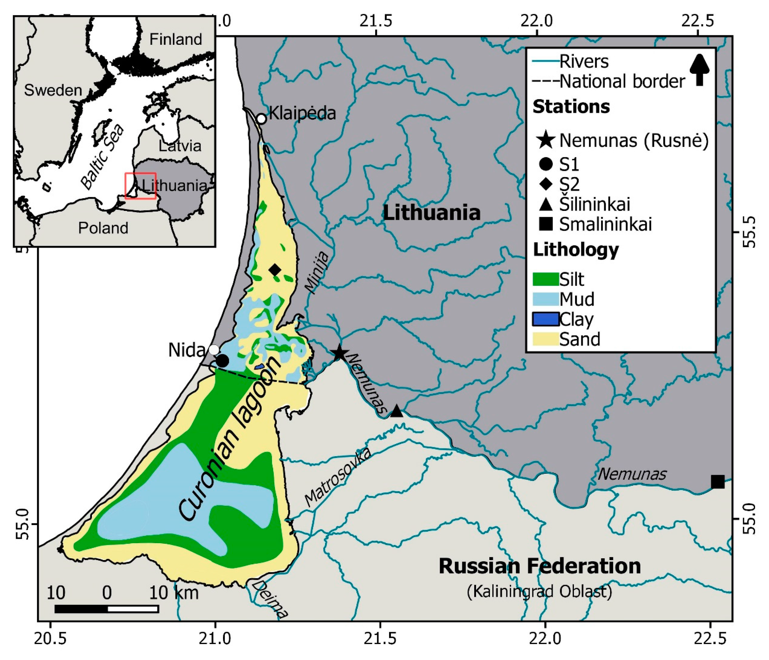
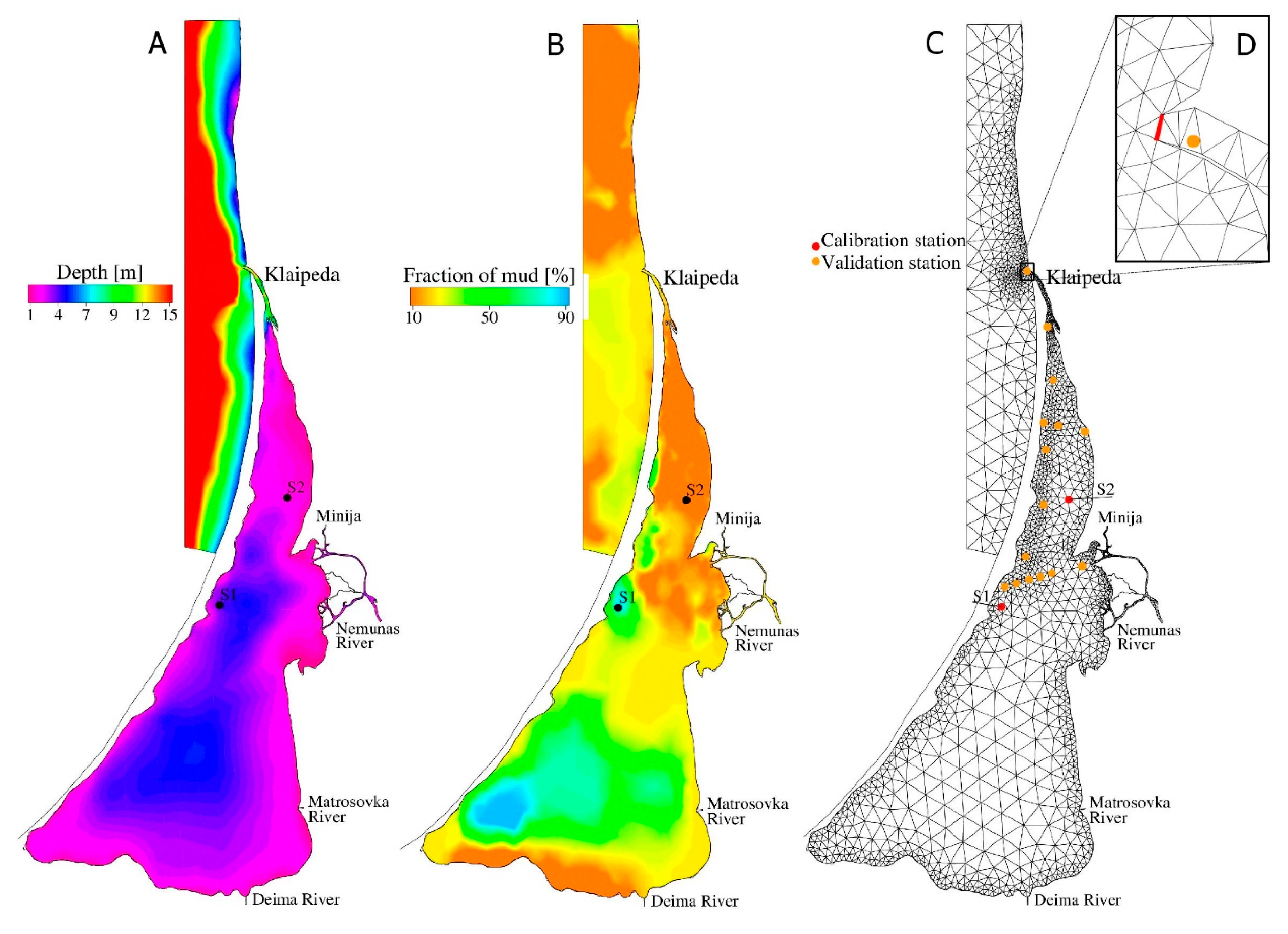
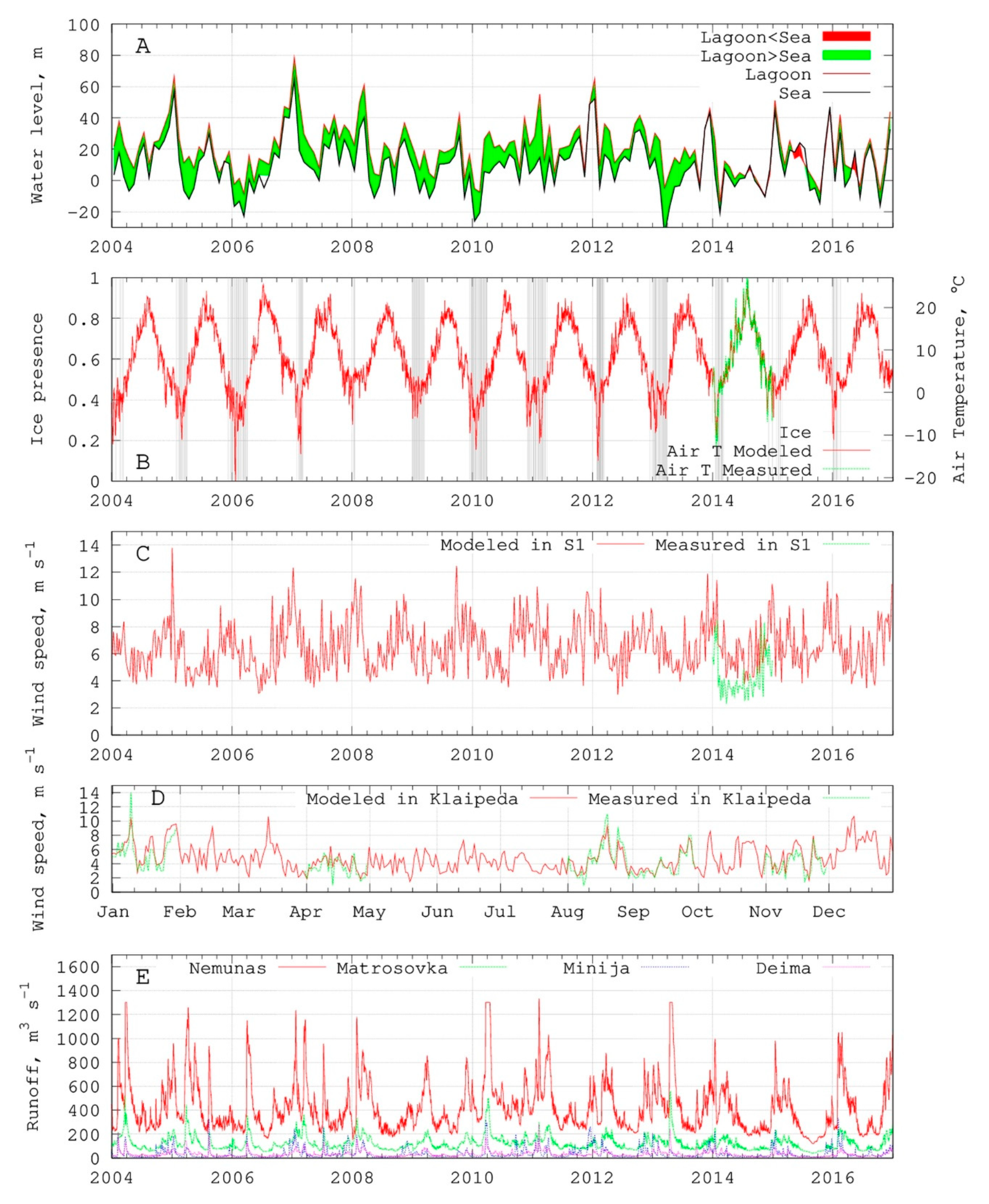
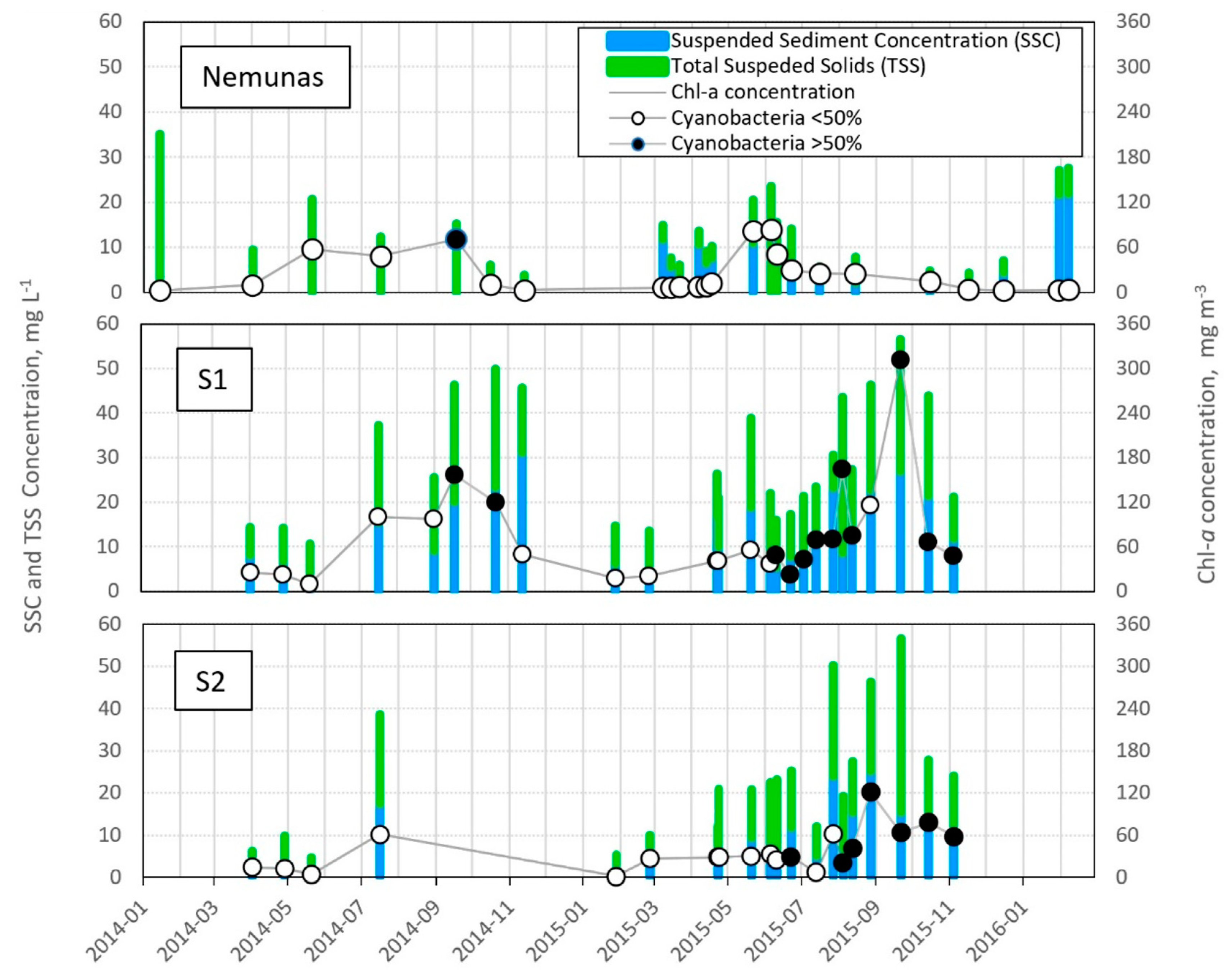
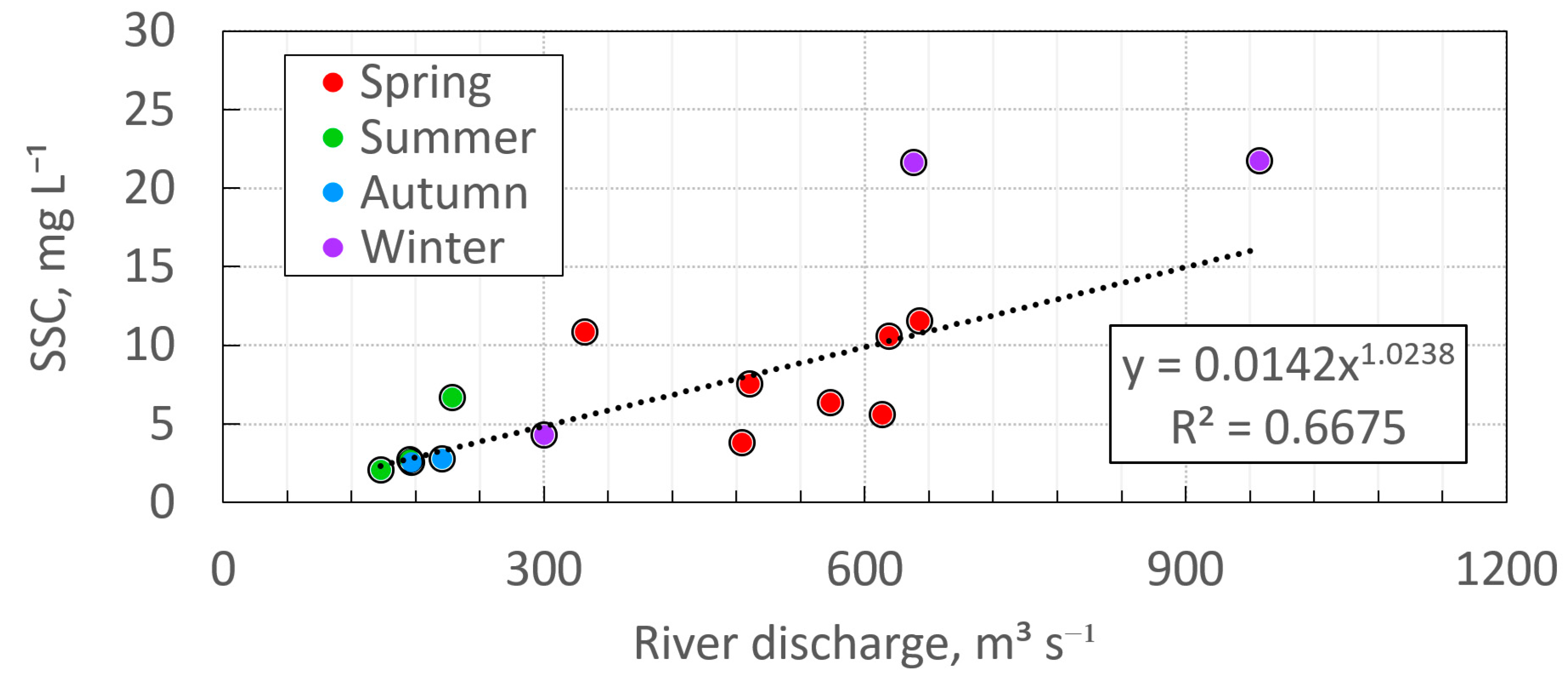
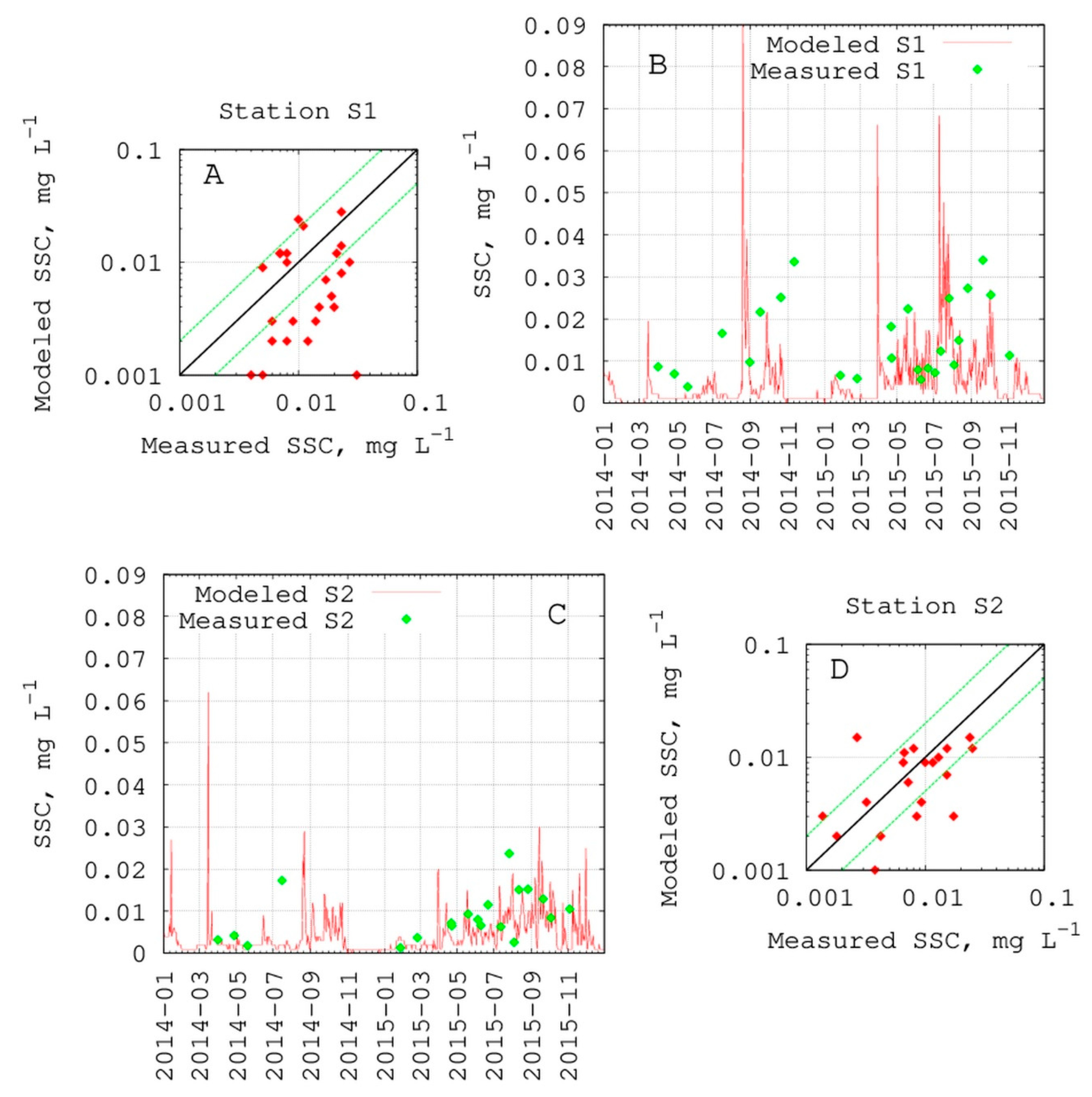
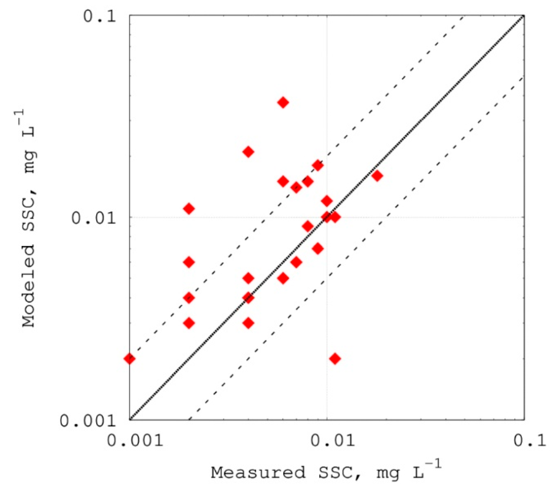
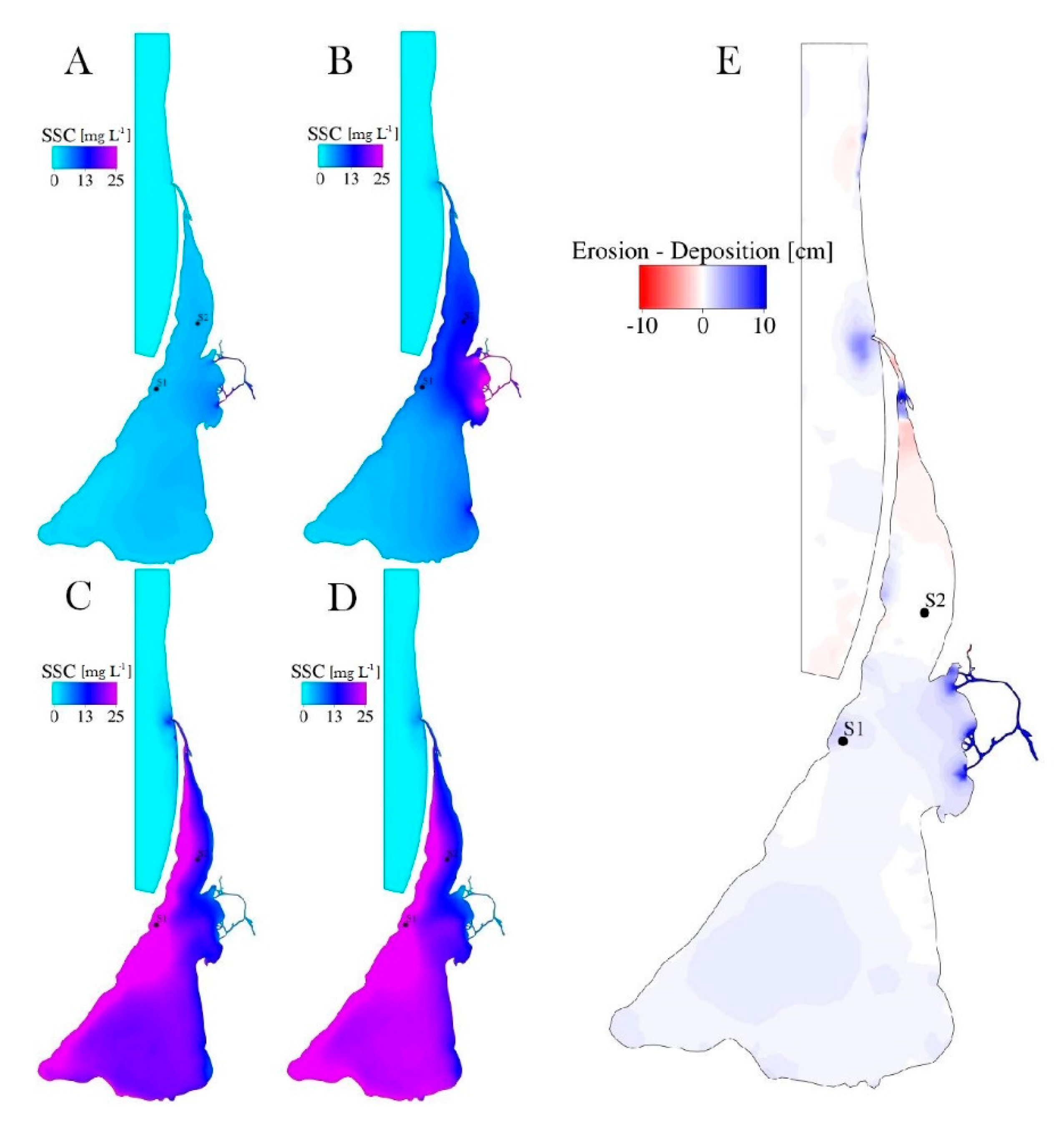
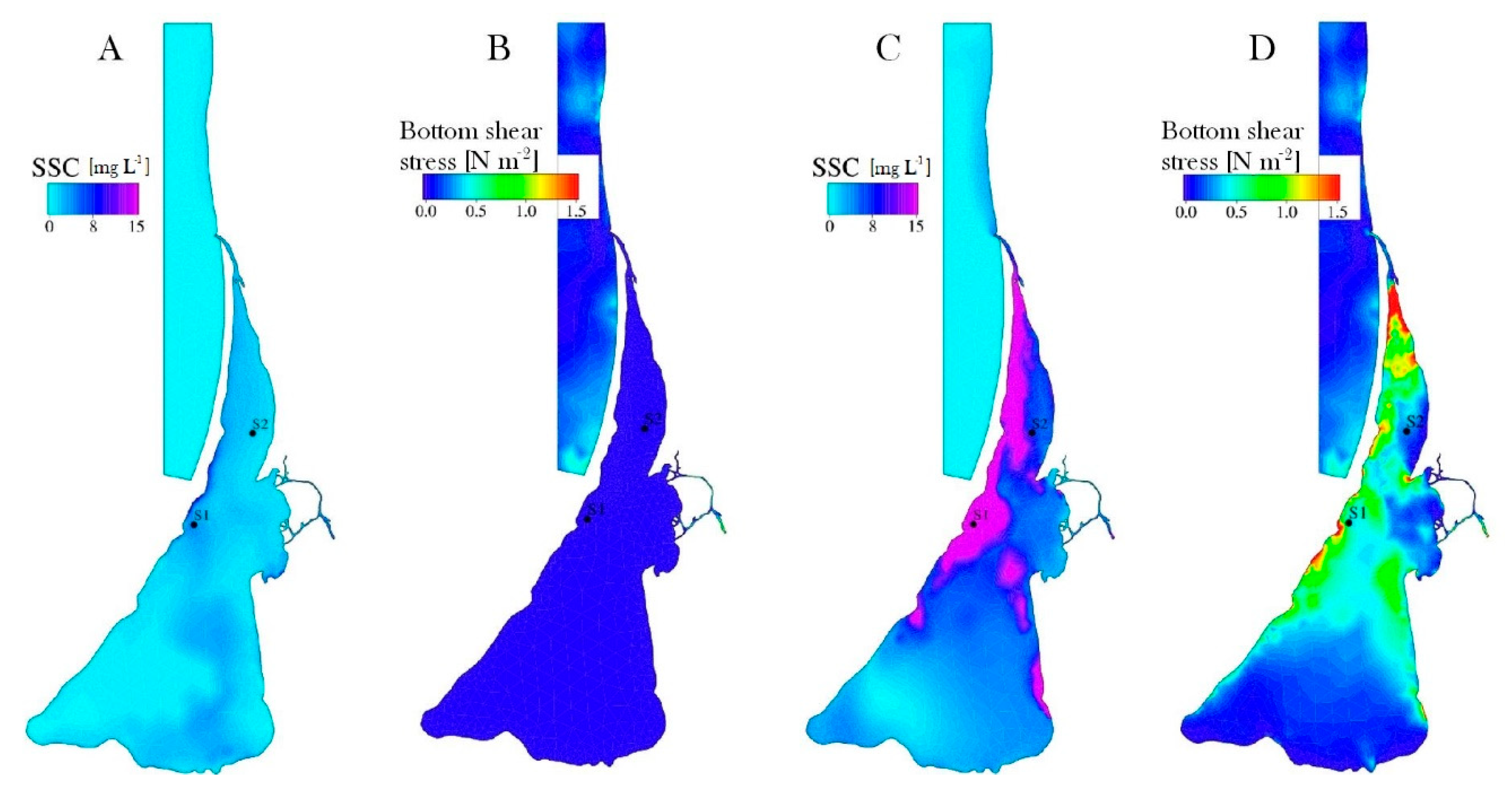
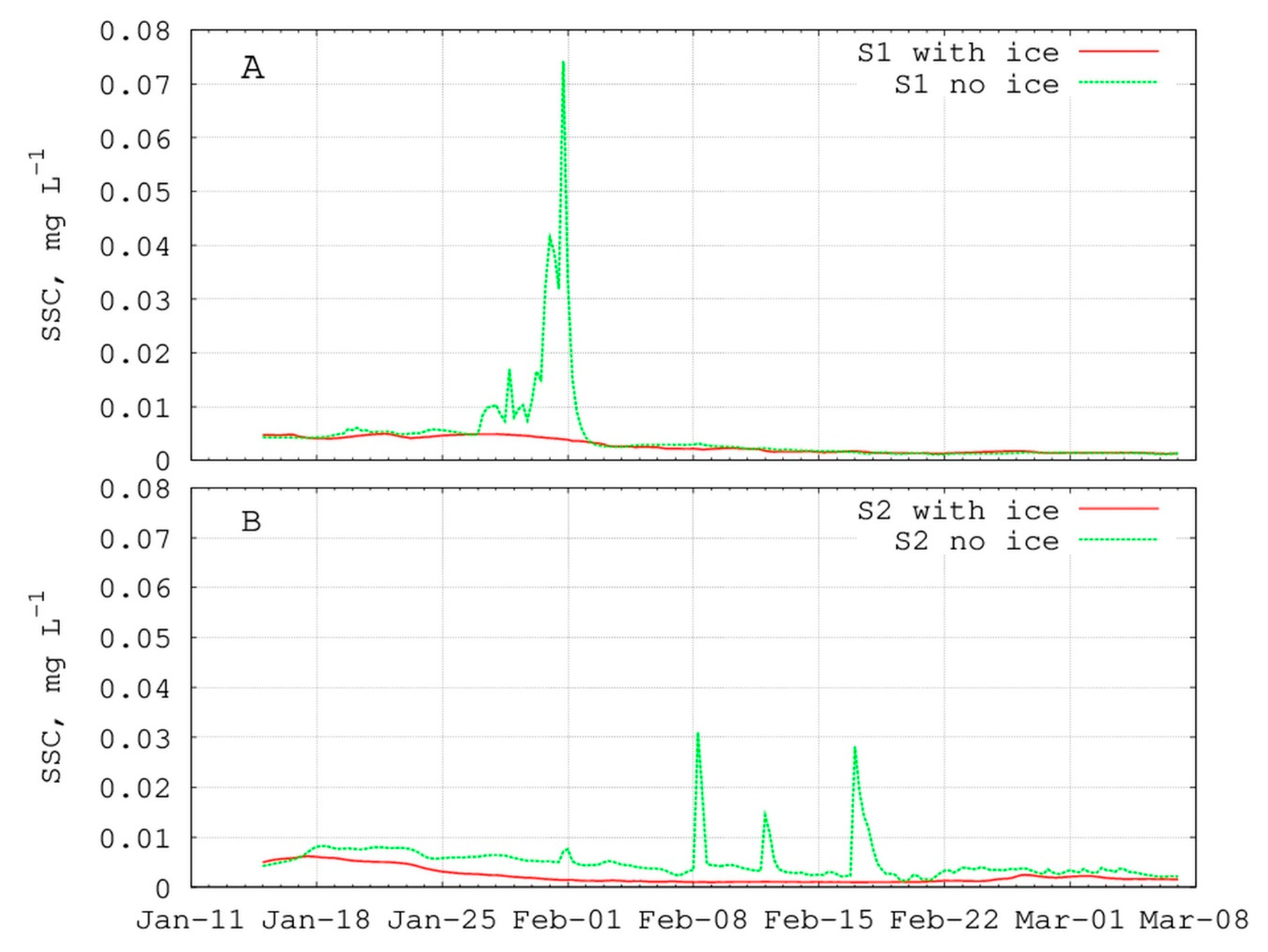
Table 1.
The main characteristics of the monitoring stations.
| Station | Location | Depth, m | Median Bottom Grain Size, µm | Percentage of Mud, % | Number of Samples |
|---|---|---|---|---|---|
| S1 | 55.286017 N | 3.35 | 35 | 77 | 25 |
| 21.021400 E | |||||
| S2 | 55.444483 N | 1.90 | 210 | 1.6 | 20 |
| 21.182733 E | |||||
| Nemunas | 55.298228 N | 2.00 | 350 | 1.8 | 24 |
| 21.380543 E |
Table 2.
The summary of the model set up data.
| Data | Period | Description |
|---|---|---|
| Open sea boundary | 2004–2006 | DHI model MIKE 21 |
| 2007–2010 | SMHI model HIROMB | |
| 2011–2013 | IOW model MOM | |
| 2014–2016 | SMHI model HIROMB | |
| Meteo forcing | 2004–2008 | ECMWF model data |
| 2009–2010 | Lithuanian hydrometeorological service model HIRLAM | |
| 2011–2016 | ECMWF model data | |
| River discharges | 2004–2016 | Lithuanian hydrometeorological service |
| Ice coverage | 2004–2016 | Satellite data provided by KU MRI |
| Initial bottom sediment composition | - | Gelumbauskaitė et al. [31] and Gulbinskas and Žaromskis [32] |
Table 3.
Summary of numerical experiments carried out in this study.
| Name | Period | Description |
|---|---|---|
| CAL | 2013–2015 | Simulation for sediment model calibration (also used for sensitivity tests) |
| VAL | 2015–2016 | Simulation for model validation |
| NoICE | 2013–2015 | As CAL, but without ice cover data |
| LONG | 2004–2016 | 13-year simulation |
© 2019 by the authors. Licensee MDPI, Basel, Switzerland. This article is an open access article distributed under the terms and conditions of the Creative Commons Attribution (CC BY) license (http://creativecommons.org/licenses/by/4.0/).
Share and Cite
MDPI and ACS Style
Mėžinė, J.; Ferrarin, C.; Vaičiūtė, D.; Idzelytė, R.; Zemlys, P.; Umgiesser, G. Sediment Transport Mechanisms in a Lagoon with High River Discharge and Sediment Loading. Water 2019, 11, 1970. https://doi.org/10.3390/w11101970
AMA Style
Mėžinė J, Ferrarin C, Vaičiūtė D, Idzelytė R, Zemlys P, Umgiesser G. Sediment Transport Mechanisms in a Lagoon with High River Discharge and Sediment Loading. Water. 2019; 11(10):1970. https://doi.org/10.3390/w11101970
Chicago/Turabian StyleMėžinė, Jovita, Christian Ferrarin, Diana Vaičiūtė, Rasa Idzelytė, Petras Zemlys, and Georg Umgiesser. 2019. "Sediment Transport Mechanisms in a Lagoon with High River Discharge and Sediment Loading" Water 11, no. 10: 1970. https://doi.org/10.3390/w11101970
Note that from the first issue of 2016, this journal uses article numbers instead of page numbers. See further details here.