Acute Water-Scarcity Monitoring for Africa
by
 ,
,
Amy McNally
1,* ,
,
Kristine Verdin
1,
Laura Harrison
2,
Augusto Getirana
3,
Jossy Jacob
4,
Shraddhanand Shukla
2,
Kristi Arsenault
1,
Christa Peters-Lidard
5 and
James P. Verdin
6 1
SAIC, Reston, VA 20190, USA and NASA GSFC, Greenbelt, MD 20771, USA
2
UC Santa Barbara Climate Hazards Center, Santa Barbara, CA 93106, USA
3
UMD ESSIC, College Park, MD 20740, USA and NASA GSFC, Greenbelt, MD 20771, USA
4
SSAI, Lanham, MD 20706, USA and NASA GSFC, Greenbelt, MD 20771, USA
5
NASA GSFC, Greenbelt, MD 20771, USA
6
USAID Office of Food for Peace, Washington, DC 20004, USA
*
Author to whom correspondence should be addressed.
Water 2019, 11(10), 1968; https://doi.org/10.3390/w11101968
Submission received: 15 August 2019
/
Revised: 11 September 2019
/
Accepted: 18 September 2019
/
Published: 21 September 2019
(This article belongs to the Special Issue Water Supply and Water Scarcity)
Abstract
:Acute and chronic water scarcity impacts four billion people, a number likely to climb with population growth and increasing demand for food and energy production. Chronic water insecurity and long-term trends are well studied at the global and regional level; however, there have not been adequate systems in place for routinely monitoring acute water scarcity. To address this gap, we developed a monthly monitoring system that computes annual water availability per capita based on hydrologic data from the Famine Early Warning System Network (FEWS NET) Land Data Assimilation System (FLDAS) and gridded population data from WorldPop. The monitoring system yields maps of acute water scarcity using monthly Falkenmark classifications and departures from the long-term mean classification. These maps are designed to serve FEWS NET monitoring objectives; however, the underlying data are publicly available and can support research on the roles of population and hydrologic change on water scarcity at sub-annual and sub-national scales.
1. Introduction
Reliable and up-to-date information about chronic and acute water scarcity is a much-needed resource for tackling regional and global water issues. An estimated four billion people currently face water scarcity [1]. By 2030 global population may reach 9 billion [2], and demands on domestic, industrial and agricultural water needs are expected to substantially increase during that time, potentially by 40% [3]. In chronic water-scarcity areas, where demand persistently or seasonally exceeds supply, higher population and increased sectoral demands will likely require new strategies to strengthen long-term resilience. For acute, shorter-term, water-scarcity issues, droughts will continue to pose challenges in many regions. For Africa, large population growth and climate change-driven projected decreases in precipitation and runoff [4] are especially concerning for future chronic and acute water scarcity. Chronic and acute water scarcity have implications for national security [5], food security [6], and for achieving sustainable development goals through the food–water–energy nexus [7]. This study describes a resource that can inform decision making on water scarcity issues. Good assessments and planning require up-to-date and accurate information [8], but despite the need, there has been a lack of near real time, acute water scarcity monitoring tools that meet these standards.
One of the first global scale indices of water scarcity was by Falkenmark [9] who computed annual water per capita (total annual runoff (m3/year)) and classified values ranging from “no stress” (>17,000 m3/person/year) to “absolute scarcity” (<500 m3/person/year). These thresholds are still commonly used and have been widely adopted given their ease of computation and interpretation. Ratios of supply-to-demand and different critical thresholds for municipal, industrial, and agricultural activities are sometimes used to identify sector-specific scarcity (e.g., [10]). Alternatively, WaterGAP [11] uses water use models to compute demand at each pixel. Pfister et al. [12] relates water withdrawals to water availability. More recently, the concept of a water footprint [13] has been used to describe sub-annual variations in water availability. In this approach, the blue water footprint represents the amount of water supplied to and consumed by domestic and industrial sectors, while the green water footprint represents the amount of water supplied to and consumed by vegetation (natural or agricultural). An added benefit is that this approach allows for the consideration of return flows from these sectors (e.g., [14]). Finally, a number of studies have examined long-term changes in water availability (e.g., [15]) and future projections of population, water use, and water supply (e.g., [16]). These are just a few indicators of chronic water scarcity that have been exhaustively reviewed [17,18,19,20]. The disadvantage of these indicators is that they are not routinely updated despite ever-changing water supply and water demand conditions.
Information about chronic water scarcity, the focus of many prior studies, is valuable for high-level policy guidance. In addition, humanitarian relief efforts require information that can provide a basis for responding to acute events, defined as a short-term phenomenon, related to a natural or human-made shock. Early identification of emerging acute water scarcity situations requires that information be reliable and timely, and thus be regularly updated at seasonal, monthly, or sub-monthly time scales. There are several hydrologic modeling systems that are used for drought monitoring, e.g., the North American Land Data Assimilation System (NLDAS) [21] and the Princeton Climate Analytics which includes the Africa Flood and Drought Monitor [22]. Monitoring systems like Princeton’s and NLDAS provide timely hydrologic information but they only address the supply side of water availability. Our objective is to produce a timely monitoring product for acute scarcity that also incorporates societal water demand.
We propose to combine insights from both the chronic water-scarcity community and the drought-monitoring community, to provide accurate and low latency (~1 month) information for acute (near-term) decision support. As noted earlier, prior studies have explored a variety of ways to estimate water demand. However, these more complicated approaches are difficult to deploy and as a result their use is often limited to the original study [19]. Specifically, some water demand data is available in a tabular format in the literature [23,24] or via The United Nation’s Food and Agriculture Organization’s (FAO) Aquastat, however to our knowledge, geospatial databases of water withdrawals and consumption are only available from the World Resources Institute’s (WRI) Aqueduct program [25]. These difficulties bring us back to the pioneering work by Falkenmark, who used population as a simple proxy for demand. This approach allows for routine monitoring of acute water scarcity to provide effective decision support while jointly considering dynamic changes in both supply and demand. In the case of the Famine Early Warning System Network (FEWS NET), monthly updated water scarcity maps have potential to provide input to monthly food assistance outlooks that support humanitarian decision making.
This paper presents a system to provide early warning and identify emerging regional hot spots for water scarcity associated with climate extremes. The system described in this paper focuses on Africa, but could be extended globally. The system’s routine hydrologic analysis is based on satellite driven inputs to hydrologic modeling simulations and monthly water availability per capita estimates. Specifically we use the FEWS NET Land Data Assimilation System (FLDAS [26]) driven with Climate Hazards Group InfraRed Precipitation with Stations (CHIRPS) [27] rainfall, gridded population data, and a novel formulation of the Falkenmark Index. Given the lack of reliable, high-resolution water-use data, we use high-resolution population estimates from 2015 to inform water management in near real time. As described in the Materials and Methods section, the system builds upon FLDAS drought monitoring capabilities to also support investigations into human water scarcity.
The Results section demonstrates applications of our water scarcity index beginning with the Kariba Dam on the border of Zambia and Zimbabwe which experienced extreme dry conditions in 2019. Next, we ask questions regarding the sensitivity of water scarcity to both supply and demand. Specifically, we ask: over continental Africa, (1) how has water scarcity changed over time as a function of changes in streamflow? (2) How has water scarcity changed over time as a function of changes in population? Then for the Lake Victoria basin, where human pressures are challenging water managers [28], we explore the combined impacts of both streamflow and population change and how that manifests in our water scarcity index. We conclude with a discussion of strengths and weaknesses of our approach and avenues for future work and improvements.
2. Materials and Methods
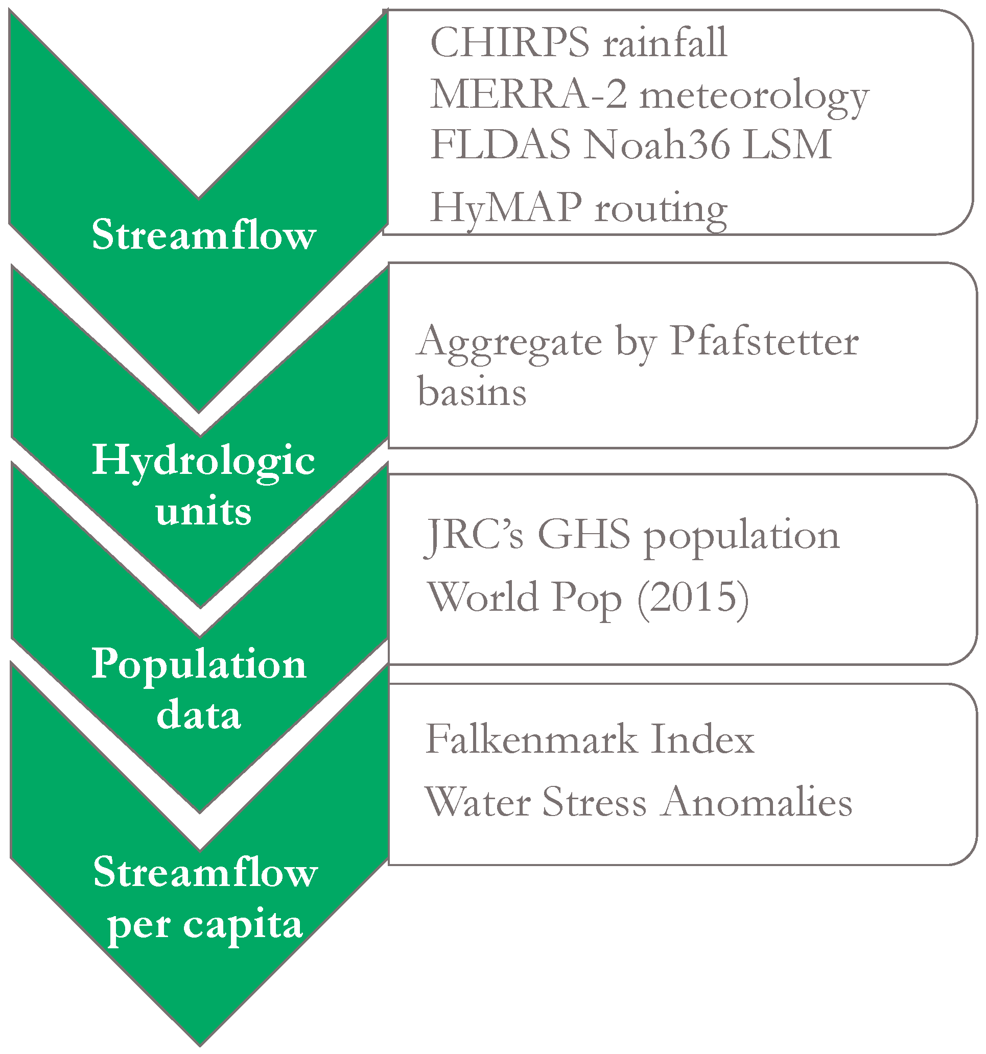
We base routine water scarcity mapping (Figure 1) on outputs from the FLDAS which is a custom instance of the National Aeronautics and Space Administration (NASA) Land Information System (LIS [29]). The FLDAS’s Noah 3.6 land surface model [30] is driven by CHIRPS rainfall [27] and NASA’s Modern-Era Retrospective analysis for Research and Applications (MERRA-2) meteorological forcing [31]. The model partitions rainfall inputs into evapotranspiration, soil moisture storage, surface and subsurface runoff (i.e., baseflow). Surface runoff results from precipitation in excess of saturation and infiltration capacity, while subsurface runoff is gravity drainage from the bottom soil moisture layer. The sum, or total runoff, is routed through the river network with the Hydrologic Modeling and Analysis Platform version 2 (HyMAP-2) river routing scheme [32,33] using the local inertia formulation [34] to simulate surface water dynamics, including streamflow (m3/s), in rivers and floodplains.
To define catchments we use boundaries from the U.S. Geological Survey (USGS) Hydrologic Derivatives for Modeling Applications (HDMA) database [35]. Catchments are attributed with Pfafstetter codes, based on a hierarchical numbering system, that carry important topological information. For instance, the Nile Basin is Pfafstetter level 1, and the Blue Nile basin is Pfafstetter level 2. For this application, we use Pfafstetter level 6 basins, to represent the relatively local nature of water supplies.
As a proxy for water demand, and consistent with the Falkenmark index, we use two population datasets. We use the WorldPop 2015 data [36] for routine mapping since these data provide better definition of the population distribution within the Pfafstetter level 6 basins than other data that we explored. For research questions regarding changes in population and water availability over time, we used the European Commission’s Joint Research Center’s (JRC) Global Human Settlement (GHS) data ([8]). These data are available for 1990, 2000 and 2015. Future work will explore how to use these data for time varying population in the routine scarcity maps, which will provide context to users on how both the changes in population and hydrology manifest as current water stress conditions.
As a proxy for demand, we found population to be adequate because, first, withdrawal intensity and population have the same spatial patterns. Second, population data are available for different points in time and, third, a goal of this effort was to produce an operational framework where alternative datasets can be tested in the future. We explored using the water withdrawals and consumptive use datasets generated by the WRI Aqueduct program [25]. However, we had difficulty reconciling the magnitude of streamflow simulations with WRI withdrawal and consumptive values. Our attempt at using sub-national data on surface water and groundwater use estimates (i.e., blue water footprint [13]) by sector [24] also was challenging because the data were not mapped. These and other alternatives should be explored for future efforts to better capture water demands from agriculture and other sectors.
The data and models used in our system, summarized in Table 1, are publicly available, with the exception of the HyMAP-2 river routing scheme, associated parameters, and streamflow outputs. HyMAP-2 and parameters are anticipated to be in a future LIS release, but is still in development at the time of this study. MERRA-2 and monthly FLDAS outputs are provided by the NASA Goddard Earth Sciences Data and Information Services Center (GES DISC). While the spatial domain for all of the inputs is global, for initial development of this routine water scarcity mapping workflow we focused on the Africa domain where many FEWS NET countries of interest are located.
Using these inputs, we developed a new, modified version of the Falkenmark Index for routine water scarcity monitoring. Falkenmark Index thresholds (Table 2) are specified annually, however, we required monthly updates of scarcity conditions. To accomplish this, we used a 12-month running total of the streamflow from the current and 11 previous months. This allowed us to use the standard Falkenmark thresholds while also reflecting the most up-to-date water scarcity conditions. We found this 12-month running-total approach to be superior to a simple monthly calculation (dividing the thresholds by 12), which resulted in the frequency of “no stress” or “absolute scarcity” conditions being too high. The reason for this is that deficits and surpluses were not carried over from month-to-month beyond what is implicit in the hydrological models.
The final products of our analysis that appear on the NASA FEWS NET project website (https://lis.gsfc.nasa.gov/projects/fewsnet) are streamflow anomalies, the water scarcity index, and water scarcity anomalies which are calculated as follows.
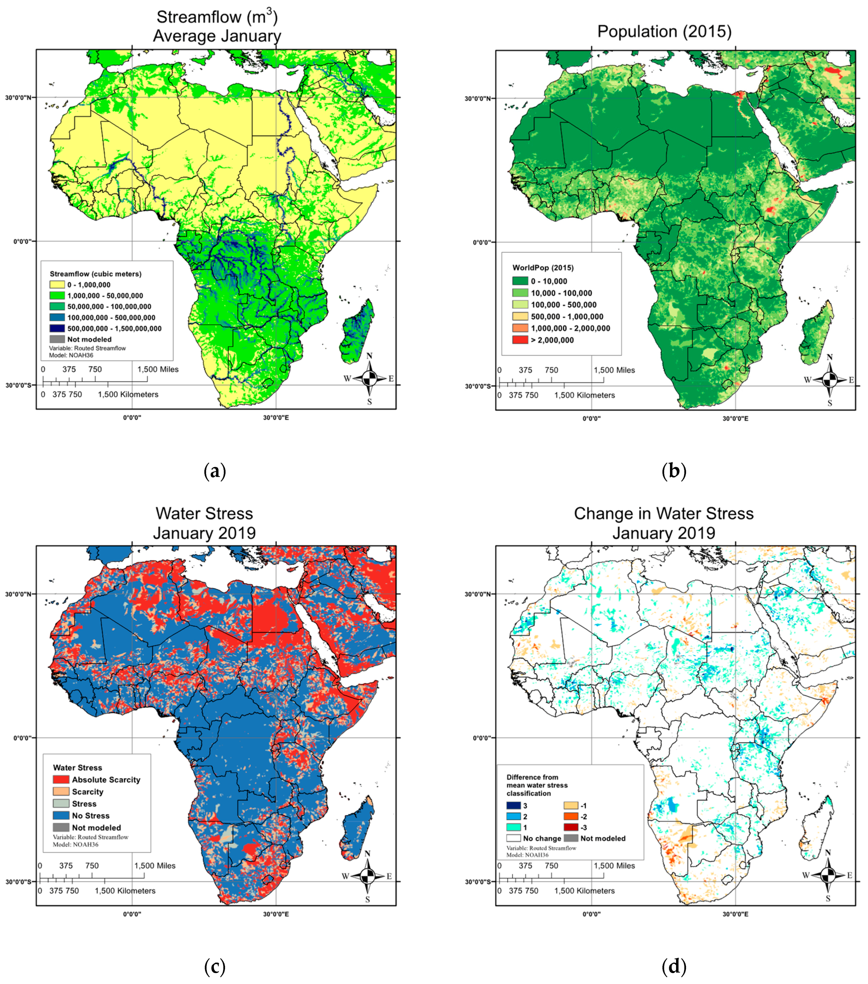
The average of the routed streamflow is calculated for each Pfafstetter basin level 6 from the HDMA database [35] and converted to a volume of water (m3/month) (Figure 2a).
Anomalies are calculated as a percent of the mean as:
where m is a given month and y is a given year. Climatologym is the mean streamflow for each 12-month period based on the 1982–2016 FLDAS historical record.
Anomaly (%) = [(streamflowm,y climatologym)/climatologym] × 100
To compute water scarcity, first, we aggregate population estimates to the Pfafstetter basin level 6 (Figure 2b). Then we divide the given 12-month total spatially aggregated streamflow (m3) by the population to produce an estimate of m3/person. We then produce maps where each basin’s water availability is classified by the values in Table 2 (Figure 2c).
Next, to highlight acute water scarcity conditions, we map the departure from average conditions for that 12-month period. Average water scarcity conditions are based on the ratio of the climatological mean 12-month streamflow total (1982–2016 FLDAS simulations) and the most recent 2015 WorldPop population. Water scarcity for both climatology and the current month is assigned a numeric value 1–4 (absolute scarcity to no stress, following categories listed in Table 2), which allowed us to compute the difference of the current water-scarcity classification from the climatology (Figure 2d). We show maps of the components of this system for January 2019 maps as examples of system inputs (Figure 2a,b) and outputs (Figure 2c,d). Streamflow and outputs vary by month and year, while population inputs are currently static in the system.
3. Results
The primary goal of this paper is to describe the routine water scarcity monitoring system (see Section 2. Materials and Methods), and show applications to acute water scarcity monitoring. We begin with an example for Lake Kariba, a dam along the Zambia and Zimbabwe border, where variations in measured lake levels generally correspond to time-varying information in water stress anomaly maps. We then explore combined impacts of both streamflow and population change and how that manifests in our water scarcity index, first for continental Africa, and then for the Lake Victoria basin, where human pressures are challenging water managers [28].
3.1. How Well Do the Maps Represent the Water Scarcity Events in Zambia and Zimbabwe That Affect the Kariba Dam?
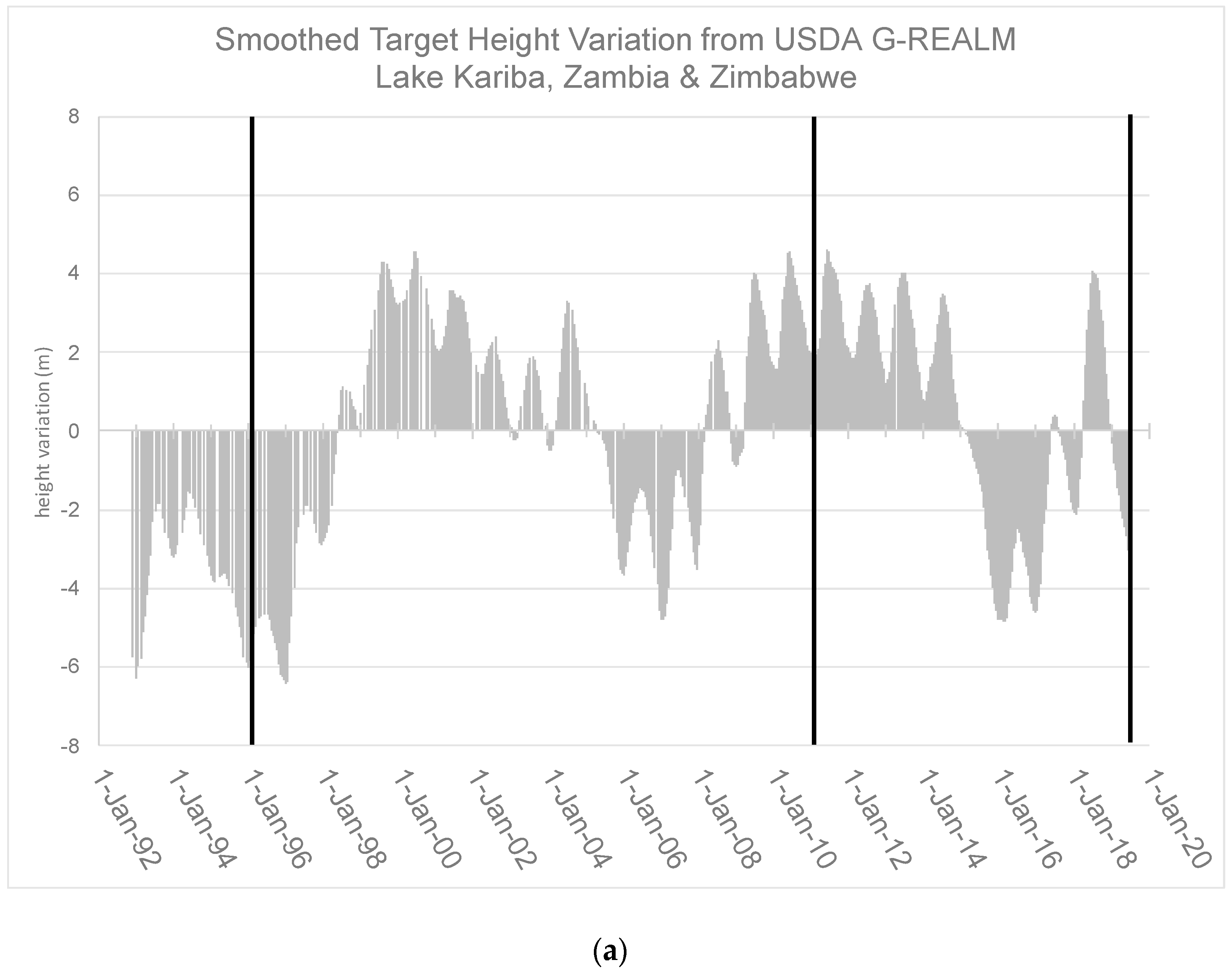
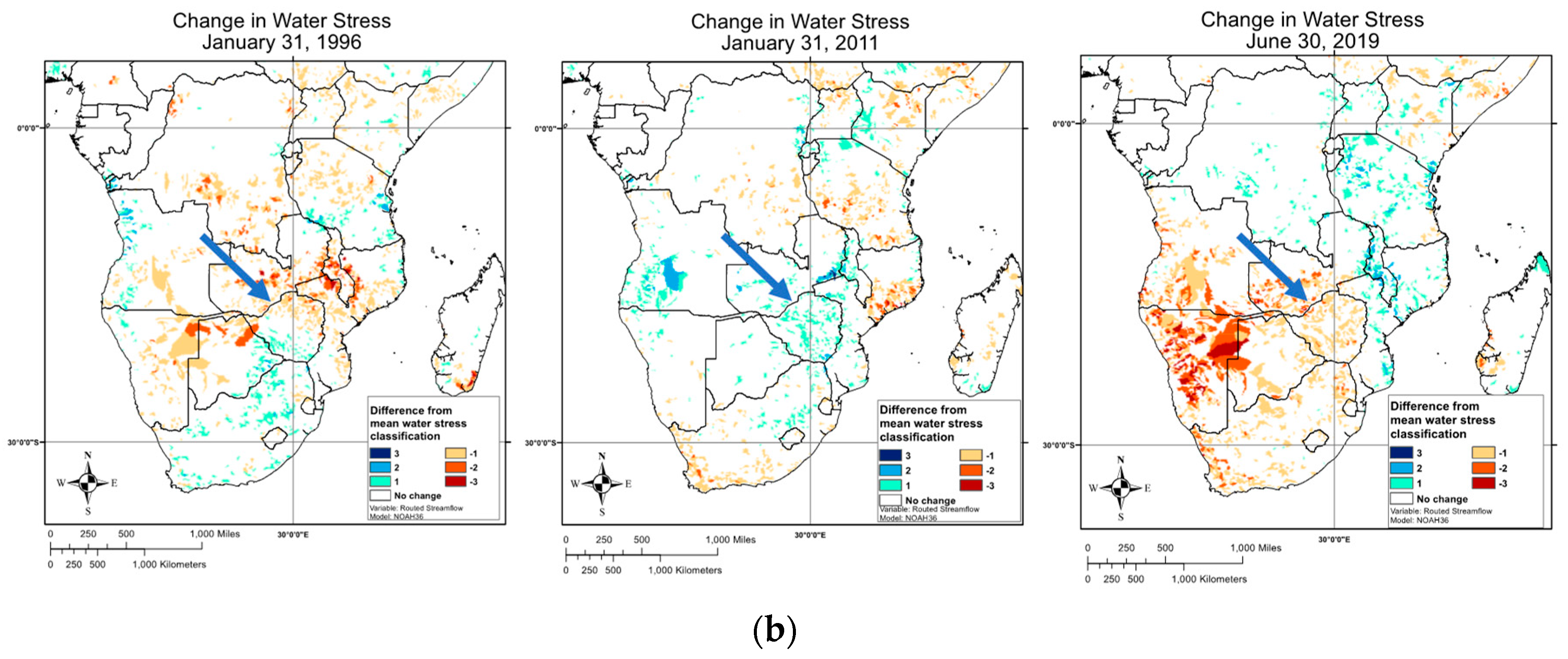
Figure 3 shows monthly observed height levels for Lake Kariba from the US Department of Agriculture (USDA) Global Reservoir and Lakes (G-REALM) project, measured by satellite altimetry data [37], and water stress maps for three selected months for comparison. According to the January 1996 map (Figure 3, bottom left) numerous basins in the southern Zambia and northern Zimbabwe region were in a water stress category that was 1–3 classes drier than would be expected in a typical January, and this corresponds with measured lower than average Lake Kariba height. In January 2011 (Figure 3, bottom middle) numerous basins in that region show water stress conditions in a more positive state than a typical January, around 1–2 classes higher than average, which corresponds to measured higher than average reservoir height at that time. Most recently, in June 2019, Figure 3 data show impacts of a drier than average 2018–2019 rainfall season on basins in the region. Dry conditions are reflected in both reservoir heights and the water stress classification. News reports from 2019 confirmed low levels (29% full [38]) in the Kariba Dam, reducing hydropower supply and threatening complete shut-down [39,40]. Water shortages were also reported in Botswana [41] in 2019 and in Namibia, where severe drought left many people without access to clean water for crops and drinking water for people and livestock [42]. The June 2019 map indicates higher than average water stress categories in these areas
3.2. How Have Water Scarcity Classes Changed over Time as a Function of Changes in Streamflow?
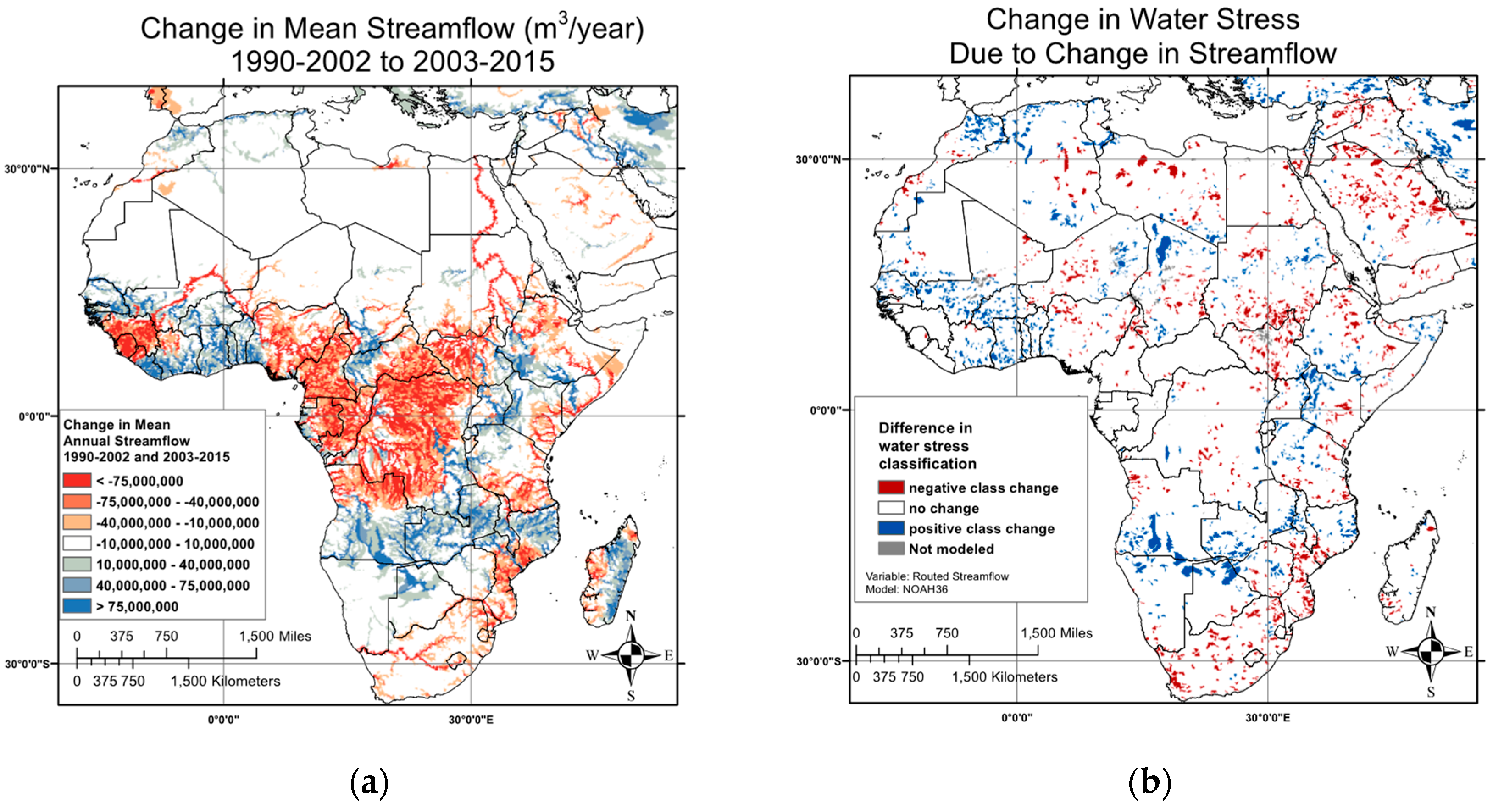
In addition to monitoring conditions, we wanted to understand how water scarcity has changed over time exclusively as a function of streamflow, holding population constant. To answer this question, first we computed the difference in mean annual streamflow for an early period (1990–2002) and a late period (2003–2015). The difference between the periods is shown in Figure 4a. Notable patterns in this figure are the decrease in streamflow for central Africa, southern Tanzania, southern Kenya, Somalia, Guinea, southern Africa, and western Madagascar. Meanwhile other regions have shown a marked increase: Lake Victoria region, Malawi, Zambia, northern Mozambique, and Ghana and neighboring countries.
We explored using a linear trend for this analysis but favor period-differences for several reasons. First, linear trends are sensitive to extreme events, particularly at the end-point of the time period. Second, linear trends are sensitive to the time period that is used, making stated trends non-robust and easy to misinterpret. A third reason is that we are particularly interested in how, over the past 20–30 years, have people been experiencing changes in water availability on a decadal scale.
The patterns in Figure 4a are generally confirmed by literature that references water availability trends estimated from the Gravity Recovery and Climate Experiment (GRACE) satellite (2002–2014). GRACE measures total water storage changes over time [43,44]. Changes in FLDAS streamflow are largely driven by increases or decreases in rainfall, which is consistent with results in Rodell et al. [43]. For example, Rodell et al. [43] and FLDAS streamflow show a wetting trend in southwestern Africa, in the Okavango Basin that includes Angola, Namibia, Botswana and Zimbabwe (Figure 4a). Farther south and east, in South Africa, eSwatini, Lethsoto, and Southern Mozambique there are drying trends due to decreasing rainfall. Both Rodell et al. and FLDAS streamflow show increases in the West African country of Ghana (and neighboring countries) with increases in rainfall. Rodell et al. attribute increases in the Lake Victoria region to increasing lake levels and groundwater. These characteristics are not modeled with FLDAS’s Noah 3.6, but are ultimately driven by increases in rainfall.
While hydrologic trends are interesting, they do not address how much these changes matter in the context of water scarcity per capita. Here we ask, what is the effect of these changes in the context of the Falkenmark Index? To answer this question, we compute the Falkenmark index for the early and the late periods and map the changes in class (Figure 4b). The positive and negative spatial patterns are generally similar, but show interesting results with respect to the scope of societal impacts. In areas with a change in water stress class, the change associated with a streamflow change is most often to a class ±1 level higher or lower. Exceptions, with more extreme class changes, are seen in a few basins in central Kenya, central Mozambique, and South Africa. Also interesting is that results do not show prominent increases in water stress associated with large streamflow declines across the Democratic Republic of the Congo (DRC), Republic of the Congo, Gabon, and Cameroon, but they do show more prominent increases in water stress in South Sudan. This is related to differences in regional hydro-climatology, with most of central-west Africa being consistently wet enough to remain in the “No Stress” Falkenmark category while less wet areas have more opportunity to transition between stress categories.
3.3. How Have Water Scarcity Classes Changed over Time as a Function of Changes in Population?
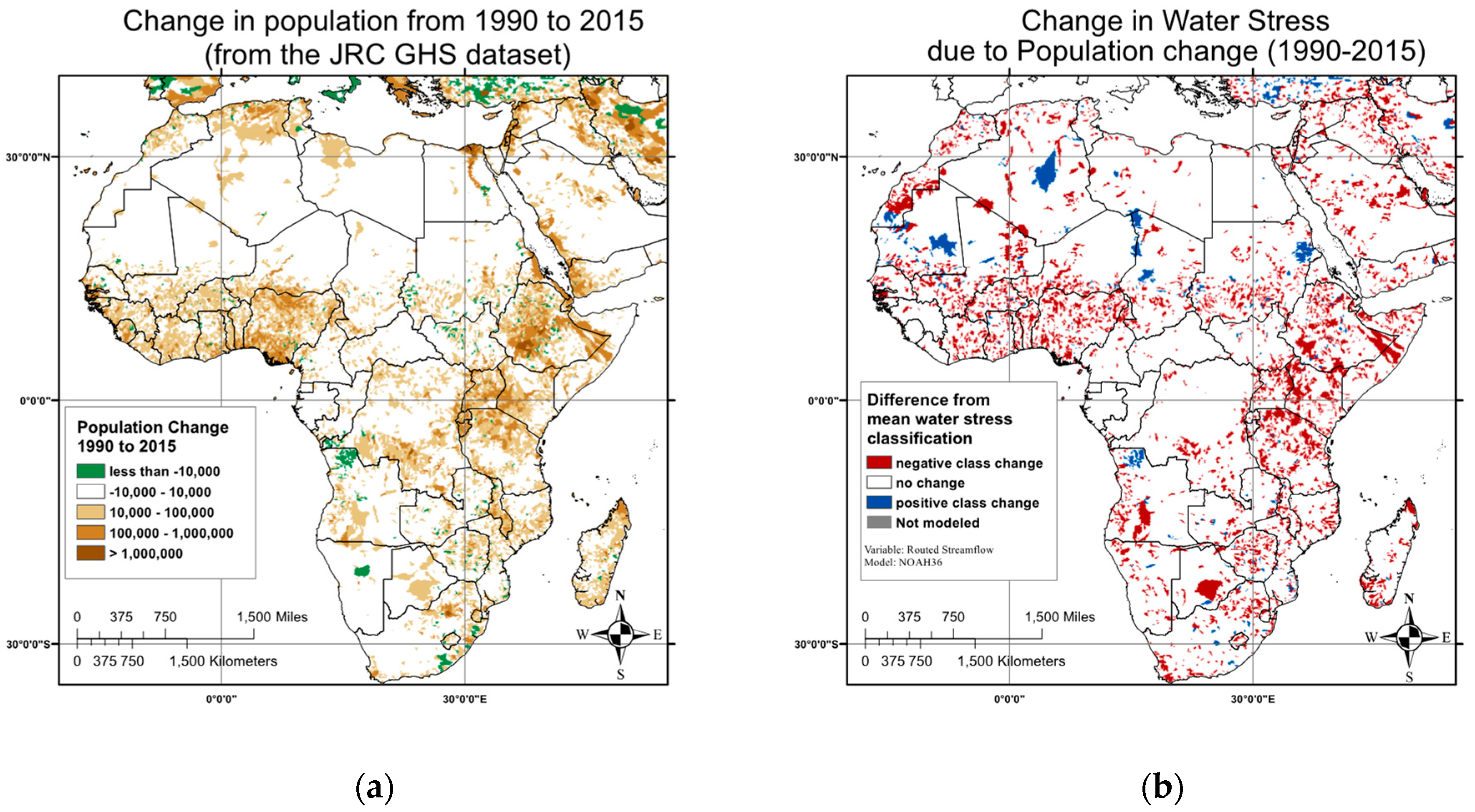
In addition to understanding changes in supply, we wanted to understand how water scarcity has changed over time as a result of demand, represented by changes in population. To answer this question, we use the average annual streamflow from 1990–2015, and computed the change in population from 1990 to 2015 using the JRC GHS data. Figure 5a shows the change in population between the two time periods, 1990–2002 and 2003–2015. Brown colors indicate increasing population, which is the case over much of the continent. Particularly high population growth is shown in Ethiopia, Nigeria, and Lake Victoria basin.
Next, we ask: what is the effect of these changes in the context of the Falkenmark Index? Patterns in the change in water scarcity maps are similar to changes in population (Figure 5b). Unlike changes in hydrology that had a ±1 class impact on water availability, changes in population results in a −1 to −3 change in water scarcity class (not shown). While population is a simplistic proxy for demand, this result highlights the importance of including demand in the analysis of hydrologic changes if the results are to be applicable to water availability. Water-rich areas like the Congo and Liberia, did not change water-scarcity category despite increasing population. However, there are water-rich areas like Tanzania and Nigeria and other parts of the Gulf of Guinea coast where despite being water rich, population pressure is intense.
3.4. How Have Water Scarcity Classes Changed over Time as a Function of Changes in Population and Changes in Hydrology in the Lake Victoria Basin?
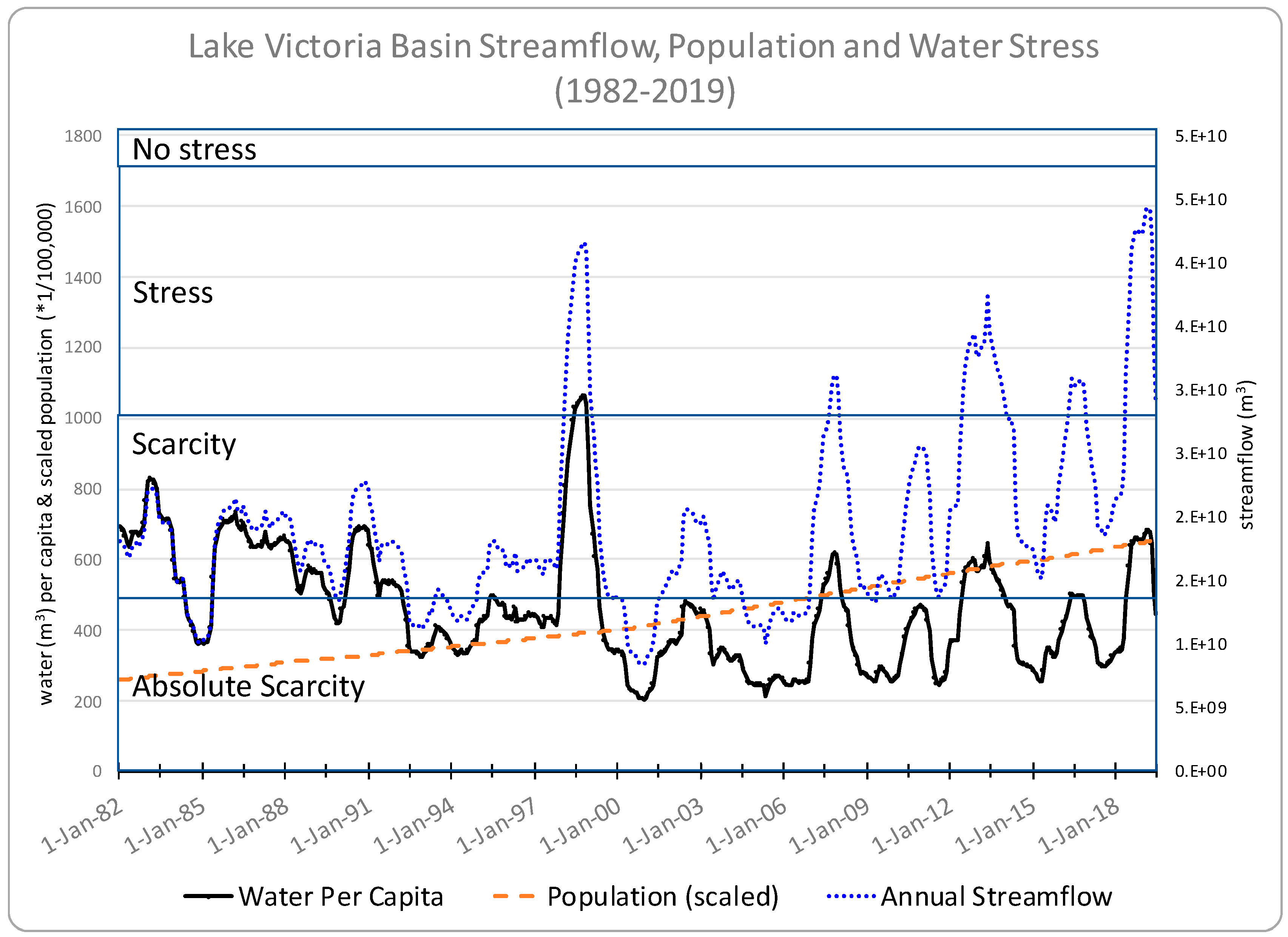
To demonstrate how changes in both population and hydrology impact water availability we use an example of the Lake Victoria Basin. In this basin, population has steadily increased since 1990, from about 400 million to 1 billion people, in 2017. Hydrologic conditions (water supply) over this time period have fluctuated with a downward trend from 1990–2009, and relatively wetter conditions from 2010–2017. A linear trend of the full time period, or differencing of two time periods (1990–2002 vs. 2003–2018) suggests no large change in water supply. When we plot population, streamflow, water scarcity, and water scarcity classes on the same figure (Figure 6) we can see that between 1990–2001 the typical classification was “stress”. From 2001–2009 the typical classification was “scarcity” with three instances of “absolute scarcity”, predominantly related to increases in population. From 2010–2017, the relatively wet period the classification improved to “scarcity” but only reached the less severe “stress” category in 2012, the wettest year in the period. This example highlights how population increases can shift scarcity categories, even in basins where hydrologic conditions are increasing water supply.
4. Discussion and Conclusions
Our modified, operational Falkenmark Index, representing the current month’s water availability based on population data and FLDAS streamflow, fills an important gap between acute drought-monitoring and chronic water-scarcity analysis. Drought monitoring efforts like NLDAS and Princeton Analytics provide routine updates regarding water supply but do not produce indices that account for water demand. We borrow from the chronic water-scarcity community to address water demand, and operationalize the Falkenmark index, traditionally based on annual water supply, by using a 12-month running total of streamflow. Our use of the Pfafstetter 6 hydrologic units further operationalizes previous water scarcity approaches by moving away from the national, or large river basin scale to compute water scarcity over smaller catchments that better represent the local nature of water availability.
This system provides monthly-updated maps of water scarcity (no stress, stress, scarcity and absolute scarcity) as well as maps that show how this classification deviates from the long-term average. These maps highlight acute water scarcity events and provide up-to-date information for decision makers who need to prioritize assistance at a regional scale and plan at a local scale. Compared to previously existing publicly available hydrologic and population datasets, this system provides decision makers with more timely information that is also interpretable, in that water stress changes can be traced back to FLDAS streamflow estimates based on CHIRPS and MERRA-2 climate inputs.
While it is difficult to validate specific locations’ water scarcity classification, our maps show similar spatial patterns of scarcity in the Horn of Africa, southern Africa, and north Africa as studies using an inverse function of annual withdrawals to availability (Water Stress Index (WSI)) [12], the ratio of withdrawals to mean annual runoff (WSI; IWMI; [45], or the withdrawal to availability ratio (WRR [46]). However, our index, and the cumulative demand to withdrawal ratio (CWD) from Hanaski et al. [46], indicates more scarcity in densely populated regions of West Africa, and scarcity in Madagascar, both of which are confirmed in news reports (e.g., Ivory Coast [47], Madagascar [48]).
Our approach does not highlight water scarcity in sparsely populated areas (e.g., the Sahara Desert, Eastern Kenya, and the Kalahari Desert), due to low population. This has been highlighted as a drawback of the Falkenmark Index, and may under-represent the severity of water insecurity for poor populations, living in marginal areas with low population density and water supply. In many studies of chronic water stress, however, regions with low population density and, therefore, a small volume of absolute water demand are often masked out e.g., [45,49]. Alternatively, scarcity mapped with blue water footprints [1] do capture these low population density areas. To operationalize this or other more complicated approaches development of a high quality, moderate spatial resolution (e.g., 10 km2) publicly available water use (consumption or withdrawals) maps, with water volumes expressed relative to a hydrologic model’s naturalized streamflow, would be useful to bridge the gap between advances in research and more applications-oriented approaches.
In our exploration of changes of streamflow and population over time we found that annual water scarcity was more sensitive to population changes (Figure 4b and Figure 5b). This is commensurate with Vorosmarty et al. [10] who highlight the expected changes to water scarcity due to climate change is far less than expected changes from population change. However, our routinely updated maps with static population show a range of ±3 classes (Figure 2). Meanwhile, the Lake Victoria Basin example (Figure 6) shows that year-to-year variation in a basin (Figure 5) changed the water stress by two classes from “absolute scarcity” to “stress”, highlighting the importance of hydrologic variability on acute water scarcity. Additional modeling experiments and studies regarding hydrologic change and its relation to landuse/landcover change could be beneficial for planning for improved water use efficiency and management.
This work did not address the limitations related to uncertainty in the hydrologic or land surface modeling highlighted by Schere and Pfister [23]. The FLDAS model is uncalibrated and relies on global soil and vegetation parameters and parameters that are a source of considerable uncertainty [50]. However, select comparisons with data from the Global Runoff Data Center show that FLDAS performs well (R > 0.70) in naturalized flow regimes and larger basins (e.g., R > 0.7 in the Orange Basin [51] and R > 0.8 in the Upper Blue Nile Basin [52]). These data are also publicly available for independent verification by interested parties, which we encourage before applying FLDAS data to local scale studies and other applications. Future work should also consider the role of additional water sources, like groundwater, in our estimate of water scarcity.
Another limitation is that our routine water-scarcity index anomaly estimates are based on static population estimates. As highlighted in the Lake Victoria Basin example even when current hydrologic conditions are similar to past years population increase will result in greater water scarcity over time. Our routine mapping does not capture this, which likely underestimates the severity of current conditions in a historical context (assuming there have been no improvements in efficiency and management). How to implement a changing population over time in an operational context and further exploration of these assumptions, could be an avenue for future research.
Despite limitations, the system we describe here provides routinely updated situational awareness of water scarcity conditions in a transparent framework. Our straightforward approach provides easy to interpret information that could be applied to other sectors such as health, food security, natural hazards, and governance.
Author Contributions
Conceptualization, A.M., J.P.V., C.P.-L., K.V. and L.H.; methodology, A.M., K.V., J.J.; software, A.G., K.A.; formal analysis, A.M., K.V.; data curation and routine operations, J.J.; writing, A.M.; writing—review and editing, L.H., S.S., K.V., A.G., C.P.-L., K.A.; visualization, K.V.; supervision, C.P.-L.; project administration, J.P.V.; funding acquisition, J.P.V., C.P.-L., A.M.
Funding
NASA—USAID FEWS NET interagency agreement, USGS-UCSB cooperative agreement for FEWS NET. NASA SERVIR Applied Sciences Team.
Acknowledgments
We acknowledge the NASA GES DISC for data curation, NASA LIS team for software development. NCCS Computing for computational resources. Narcissa Princope and Greg Husak for early discussions on water availability. Lake products are courtesy of the USDA/NASA G-REALM program at https://ipad.fas.usda.gov/cropexplorer/global_reservoir/.
Conflicts of Interest
The authors declare no conflict of interest.
References
- Mekonnen, M.M.; Hoekstra, A.Y. Four billion people facing severe water scarcity. Sci. Adv. 2016, 2, e1500323. [Google Scholar] [CrossRef] [PubMed]
- UN DESA. World Population Projected to Reach 9.7 Billion by 2050; UN DESA United Nations Department of Economic and Social Affairs: New York, NY, USA, 2015. [Google Scholar]
- US National Intelligence Council. Global Trends 2030: Alternative Worlds; Government Printing Office: Washington, DC, USA, 2013; ISBN 978-0-16-091543-7.
- Gan, T.Y.; Ito, M.; Hülsmann, S.; Qin, X.; Lu, X.X.; Liong, S.Y.; Rutschman, P.; Disse, M.; Koivusalo, H. Possible climate change/variability and human impacts, vulnerability of drought-prone regions, water resources and capacity building for Africa. Hydrol. Sci. J. 2016, 61, 1209–1226. [Google Scholar] [CrossRef]
- USAID. U.S. Government Global Water Strategy 2017; USAID: Washington, DC, USA, 2017.
- USAID. U.S. Government Global Food Security Strategy 2016; USAID: Washington, DC, USA, 2017.
- McNally, A.; McCartney, S.; Ruane, A.C.; Mladenova, I.E.; Whitcraft, A.K.; Becker-Reshef, I.; Bolten, J.D.; Peters-Lidard, C.D.; Rosenzweig, C.; Uz, S.S. Hydrologic and Agricultural Earth Observations and Modeling for the Water-Food Nexus. Front. Environ. Sci. 2019, 7, 23. [Google Scholar] [CrossRef]
- Clark, W.C.; van Kerkhoff, L.; Lebel, L.; Gallopin, G.C. Crafting usable knowledge for sustainable development. Proc. Natl. Acad. Sci. USA 2016, 113, 4570–4578. [Google Scholar] [CrossRef] [PubMed] [Green Version]
- Falkenmark, M. The Massive Water Scarcity Now Threatening Africa: Why Isn’t It Being Addressed? Ambio 1989, 18, 112–118. [Google Scholar]
- Vörösmarty, C.J.; Green, P.; Salisbury, J.; Lammers, R.B. Global water resources: Vulnerability from climate change and population growth. Science 2000, 289, 284–288. [Google Scholar] [CrossRef]
- Döll, P.; Kaspar, F.; Lehner, B. A global hydrological model for deriving water availability indicators: Model tuning and validation. J. Hydrol. 2003, 270, 105–134. [Google Scholar] [CrossRef]
- Pfister, S.; Koehler, A.; Hellweg, S. Assessing the Environmental Impacts of Freshwater Consumption in LCA. Environ. Sci. Technol. 2009, 43, 4098–4104. [Google Scholar] [CrossRef] [Green Version]
- Hoekstra, A.Y.; Mekonnen, M.M. The water footprint of humanity. Proc. Natl. Acad. Sci. USA 2012, 109, 3232–3237. [Google Scholar] [CrossRef] [Green Version]
- Wada, Y.; Wisser, D.; Bierkens, M.F.P. Global modeling of withdrawal, allocation and consumptive use of surface water and groundwater resources. Earth Syst. Dyn. 2014, 5, 15–40. [Google Scholar] [CrossRef] [Green Version]
- Donchyts, G.; Baart, F.; Winsemius, H.; Gorelick, N.; Kwadijk, J.; van de Giesen, N. Earth’s surface water change over the past 30 years. Nat. Clim. Chang. 2016, 6, 810–813. [Google Scholar] [CrossRef]
- Mankin, J.S.; Viviroli, D.; Mekonnen, M.M.; Hoekstra, A.Y.; Horton, R.M.; Smerdon, J.E.; Diffenbaugh, N.S. Influence of internal variability on population exposure to hydroclimatic changes. Environ. Res. Lett. 2017, 12, 044007. [Google Scholar] [CrossRef] [Green Version]
- Rijsberman, F.R. Water scarcity: Fact or fiction? Agric. Water Manag. 2006, 80, 5–22. [Google Scholar] [CrossRef] [Green Version]
- Brown, A.; Matlock, M.D. A review of water scarcity indices and methodologies. Food Beverage Agric. 2017, 106, 1–19. [Google Scholar]
- Liu, J.; Yang, H.; Gosling, S.N.; Kummu, M.; Flörke, M.; Pfister, S.; Hanasaki, N.; Wada, Y.; Zhang, X.; Zheng, C.; et al. Water scarcity assessments in the past, present and future. Earths Future 2017, 5, 545–559. [Google Scholar] [CrossRef] [PubMed]
- Damkjaer, S.; Taylor, R. The measurement of water scarcity: Defining a meaningful indicator. Ambio 2017, 46, 513–531. [Google Scholar] [CrossRef] [PubMed] [Green Version]
- Xia, Y.; Mitchell, K.; Ek, M.; Sheffield, J.; Cosgrove, B.; Wood, E.; Luo, L.; Alonge, C.; Wei, H.; Meng, J.; et al. Continental-scale water and energy flux analysis and validation for the North American Land Data Assimilation System project phase 2 (NLDAS-2): 1. Intercomparison and application of model products. J. Geophys. Res. Atmos. 2012, 117. [Google Scholar] [CrossRef]
- Sheffield, J.; Wood, E.F.; Chaney, N.; Guan, K.; Sadri, S.; Yuan, X.; Olang, L.; Amani, A.; Ali, A.; Demuth, S.; et al. A Drought Monitoring and Forecasting System for Sub-Sahara African Water Resources and Food Security. Bull. Amer. Meteor. Soc. 2013, 95, 861–882. [Google Scholar] [CrossRef]
- Scherer, L.; Pfister, S. Dealing with uncertainty in water scarcity footprints. Environ. Res. Lett. 2016, 11, 054008. [Google Scholar] [CrossRef] [Green Version]
- Mekonnen, M.M.; Hoekstra, A.Y. The green, blue and grey water footprint of crops and derived crop products. Hydrol. Earth Syst. Sci. 2011, 15, 1577–1600. [Google Scholar] [CrossRef] [Green Version]
- Reig, P.; Shiao, T.; Gassert, F. Aqueduct Water Risk Framework; WRI Working Paper; World Resources Institute: Washington, DC, USA, 2013. [Google Scholar]
- McNally, A.; Arsenault, K.; Kumar, S.; Shukla, S.; Peterson, P.; Wang, S.; Funk, C.; Peters-lidard, C.D.; Verdin, J.P. A land data assimilation system for sub-Saharan Africa food and water security applications. Sci. Data Lond. 2017, 4, 170012. [Google Scholar] [CrossRef] [PubMed] [Green Version]
- Funk, C.; Peterson, P.; Landsfeld, M.; Pedreros, D.; Verdin, J.; Shukla, S.; Husak, G.; Rowland, J.; Harrison, L.; Hoell, A.; et al. The climate hazards infrared precipitation with stations–A new environmental record for monitoring extremes. Sci. Data 2015, 2, 150066. [Google Scholar] [CrossRef] [PubMed]
- Juma, D.W.; Wang, H.; Li, F. Impacts of population growth and economic development on water quality of a lake: Case study of Lake Victoria Kenya water. Environ. Sci. Pollut. Res. 2014, 21, 5737–5746. [Google Scholar] [CrossRef] [PubMed]
- Peters-Lidard, C.D.; Houser, P.R.; Tian, Y.; Kumar, S.V.; Geiger, J.; Olden, S.; Lighty, L.; Doty, B.; Dirmeyer, P.; Adams, J.; et al. High-performance Earth system modeling with NASA/GSFC’s Land Information System. Innov. Syst. Softw. Eng. 2007, 3, 157–165. [Google Scholar] [CrossRef]
- Ek, M.B.; Mitchell, K.E.; Lin, Y.; Rogers, E.; Grunmann, P.; Koren, V.; Gayno, G.; Tarpley, J.D. Implementation of Noah land surface model advances in the National Centers for Environmental Prediction operational mesoscale Eta model. J. Geophys. Res. Atmos. 2003, 108. [Google Scholar] [CrossRef]
- Gelaro, R.; McCarty, W.; Suárez, M.J.; Todling, R.; Molod, A.; Takacs, L.; Randles, C.A.; Darmenov, A.; Bosilovich, M.G.; Reichle, R.; et al. The Modern-Era Retrospective Analysis for Research and Applications, Version 2 (MERRA-2). J. Clim. 2017, 30, 5419–5454. [Google Scholar] [CrossRef]
- Getirana, A.; Peters-Lidard, C.; Rodell, M.; Bates, P.D. Trade-off between cost and accuracy in large-scale surface water dynamic modeling. Water Resour. Res. 2017, 53, 4942–4955. [Google Scholar] [CrossRef]
- Getirana, A.C.V.; Boone, A.; Yamazaki, D.; Decharme, B.; Papa, F.; Mognard, N. The Hydrological Modeling and Analysis Platform (HyMAP): Evaluation in the Amazon Basin. J. Hydrometeor. 2012, 13, 1641–1665. [Google Scholar] [CrossRef] [Green Version]
- Bates, P.D.; Horritt, M.S.; Fewtrell, T.J. A simple inertial formulation of the shallow water equations for efficient two-dimensional flood inundation modelling. J. Hydrol. 2010, 387, 33–45. [Google Scholar] [CrossRef]
- Verdin, K.L. Hydrologic Derivatives for Modeling and Analysis—A New Global High-Resolution Database; Data Series; U.S. Geological Survey: Reston, VA, USA, 2017; p. 24.
- Linard, C.; Gilbert, M.; Snow, R.W.; Noor, A.M.; Tatem, A.J. Population Distribution, Settlement Patterns and Accessibility across Africa in 2010. PLoS ONE 2012, 7, e31743. [Google Scholar] [CrossRef]
- Birkett, C.; Reynolds, C.; Beckley, B.; Doorn, B. From Research to Operations: The USDA Global Reservoir and Lake Monitor. In Coastal Altimetry; Vignudelli, S., Kostianoy, A.G., Cipollini, P., Benveniste, J., Eds.; Springer: Berlin/Heidelberg, Germany, 2011; pp. 19–50. ISBN 978-3-642-12796-0. [Google Scholar]
- Latham, B.; Nhamire, B. Zimbabwe, Mozambique in power deal that could close Kariba hydro plant. Business Day, 11 July 2019. [Google Scholar]
- Ndlovu, M. Kariba Dam left with 4 metres before switching off. Bulawayo 24 News, 30 June 2019. [Google Scholar]
- Crecey, K. Power production on the verge of shutdown at Zim’s Kariba Dam. Fin24, 31 May 2019. [Google Scholar]
- Baaitse, F. Water finally flows in Shashe ward. The Okavanogo Voice, 18 June 2019. [Google Scholar]
- Episcopal Relief and Development Responding to the Drought in Namibia. Reliefweb, 26 June 2019.
- Rodell, M.; Famiglietti, J.S.; Wiese, D.N.; Reager, J.T.; Beaudoing, H.K.; Landerer, F.W.; Lo, M.-H. Emerging trends in global freshwater availability. Nature 2018, 557, 651. [Google Scholar] [CrossRef]
- Scanlon, B.R.; Zhang, Z.; Save, H.; Sun, A.Y.; Schmied, H.M.; van Beek, L.P.H.; Wiese, D.N.; Wada, Y.; Long, D.; Reedy, R.C.; et al. Global models underestimate large decadal declining and rising water storage trends relative to GRACE satellite data. Proc. Natl. Acad. Sci. USA 2018, 115, E1080–E1089. [Google Scholar] [CrossRef] [Green Version]
- Smakhtin, V.U.; Revenga, C.; Doll, P. Taking into Account Environmental Water Requirements in Global-Scale Water Resources Assessments; International Water Management Institute (IWMI), Comprehensive Assessment Secretariat: Colombo, Sri Lanka, 2004. [Google Scholar]
- Hanasaki, N.; Kanae, S.; Oki, T.; Masuda, K.; Motoya, K.; Shirakawa, N.; Shen, Y.; Tanaka, K. An integrated model for the assessment of global water resources—Part 2: Applications and assessments. Hydrol. Earth Syst. Sci. 2008, 12, 1027–1037. [Google Scholar] [CrossRef]
- Dontoh, E.; Cohen, M. Africa’s Booming Cities Are Running Out of Water. Bloomberg, 18 March 2019. [Google Scholar]
- Mosbergen, D. After 3 Years of Drought, A Starving Madagascar Teeters on The Brink Of “Catastrophe”. Available online: https://www.huffpost.com/entry/madagascar-drought-hunger_n_580dbb32e4b0a03911ed7540 (accessed on 15 August 2019).
- Vörösmarty, C.J.; Douglas, E.M.; Green, P.A.; Revenga, C. Geospatial indicators of emerging water stress: An application to Africa. Ambio 2005, 34, 230–236. [Google Scholar] [CrossRef]
- Nearing, G.S.; Mocko, D.M.; Peters-Lidard, C.D.; Kumar, S.V.; Xia, Y. Benchmarking NLDAS-2 Soil Moisture and Evapotranspiration to Separate Uncertainty Contributions. J. Hydrometeor. 2016, 17, 745–759. [Google Scholar] [CrossRef]
- McNally, A.; Verdin, K.; Jung, H.C.; Harrison, L.; Shukla, S.; Peters-Lidard, C. Hydrologic Modeling for Monitoring Water Availability in Sub-Saharan Africa; American Geophysical Union: Washington, DC, USA, 2017. [Google Scholar]
- Jung, H.C.; Getirana, A.; Policelli, F.; McNally, A.; Arsenault, K.R.; Kumar, S.; Tadesse, T.; Peters-Lidard, C.D. Upper Blue Nile basin water budget from a multi-model perspective. J. Hydrol. 2017, 555, 535–546. [Google Scholar] [CrossRef] [Green Version]
Figure 1.
Our approach for water scarcity monitoring for Africa, with the Climate Hazards Group InfraRed Precipitation with Stations (CHIRPS) rainfall and Modern-Era Retrospective analysis for Research and Applications (MERRA-2) meteorological estimates used as input to the Famine Early Warning System Network Land Data Assimilation System (FLDAS) Noah 3.6 + Hydrologic Modeling and Analysis Platform (HyMap) routing scheme. Streamflow and population estimates are aggregated by Pfafstetter basins before computing Falkenmark water-scarcity categories, and water-scarcity anomalies. Routinely updated at https://lis.gsfc.nasa.gov/projects/fewsnet.

Figure 2.
The components of the Africa water scarcity monitoring scheme using average January streamflow as an example: (a) Streamflow for January plus 11 previous months, averaged over Pfafstetter 6 basin units; (b) WorldPop 2015 population density averaged over Pfafstetter 6 basin units; (c) example map of the Falkenmark Index categories in January 2019; (d) Example map showing January 2019 departures from average January conditions, highlighting acute events.

Figure 3.
(a) US Department of Agriculture (USDA) Global Reservoir and Lakes (G-REALM) altimetry data for Lake Kariba, located on the border with Zambia and Zimbabwe, black lines denote dates shown in maps. (b) Maps of change in water stress class with respect to average. Blue arrow denotes location of Kariba Dam.


Figure 4.
(a) Difference in mean annual streamflow between 1990–2002 and 2003–2015; (b) change in Falkenmark water-scarcity class due to hydrologic change (using WorldPop 2015 population). Change is ±1 class following patterns in streamflow change, with the exception of a few basins in central Kenya, central Mozambique, and South Africa.

Figure 5.
(a) Change in population between 1990–2002 and 2003–2015 from the JRC Global Human Settlement (GHS) dataset. Population is largely increasing, some places more than others. Ethiopia, Nigeria and Lake Victoria basins are notable; (b) using average streamflow conditions the effect of population has been to increase water scarcity. Change in classification due to population change is almost exclusively negative (i.e., scarcer).

Figure 6.
Time series of the Lake Victoria Basin showing changes in streamflow, population and water scarcity classification. The blue line shows annual streamflow at the mouth of Lake Victoria basin, with a positive trend since 2000. The orange line shows the total basin population, values interpolated from 1975, 1990, 2000, and 2015 GHS estimates. The black line is water availability per capita. Color blocks denote Falkenmark thresholds (Table 2). Despite the positive trend in streamflow since 2000, water available per capita has not increased.


Table 1.
Datasets used for routine water scarcity mapping.
| Dataset or Model | Description | Data Citation | Data Availability |
|---|---|---|---|
| Climate Hazards Center InfraRed Precipitation with Station data (CHIRPS) rainfall | input to FEWS NET Land Data Assimilation System (FLDAS), available 1981–present | Funk et al. 2015 [27] | University of California, Santa Barbara (UCSB) |
| Modern-Era Retrospective analysis for Research and Applications Version 2 (MERRA-2) meteorology | input to FLDAS, availability 1979–present | Gelaro et al. 2017 [31] | NASA Goddard Earth Sciences Data and Information Services Center (GES DISC) |
| U.S. Geological Survey (USGS) Hydrologic Derivatives for Modeling and Applications (HDMA) basins | used for spatial aggregation | Verdin 2017 [35] | USGS |
| WorldPop | 2015 population estimate | Linard et al. 2015 [36] | WorldPop |
| FLDAS-Noah.36 | land surface model, monthly outputs available 1982–present | McNally et al. 2017 [26] | NASA GES DISC |
| Hydrologic Modeling and Analysis Platform (HyMAP-2) routing | river routing scheme, beta version | Getirana et al. 2012 [33]; 2017 [32] | NA |
Table 2.
Falkenmark categories.
| Category | m3/year/capita |
|---|---|
| no stress | >1700 |
| stress | 1000–1700 |
| scarcity | 500–1000 |
| absolute scarcity | <500 |
© 2019 by the authors. Licensee MDPI, Basel, Switzerland. This article is an open access article distributed under the terms and conditions of the Creative Commons Attribution (CC BY) license (http://creativecommons.org/licenses/by/4.0/).
Share and Cite
MDPI and ACS Style
McNally, A.; Verdin, K.; Harrison, L.; Getirana, A.; Jacob, J.; Shukla, S.; Arsenault, K.; Peters-Lidard, C.; Verdin, J.P. Acute Water-Scarcity Monitoring for Africa. Water 2019, 11, 1968. https://doi.org/10.3390/w11101968
AMA Style
McNally A, Verdin K, Harrison L, Getirana A, Jacob J, Shukla S, Arsenault K, Peters-Lidard C, Verdin JP. Acute Water-Scarcity Monitoring for Africa. Water. 2019; 11(10):1968. https://doi.org/10.3390/w11101968
Chicago/Turabian StyleMcNally, Amy, Kristine Verdin, Laura Harrison, Augusto Getirana, Jossy Jacob, Shraddhanand Shukla, Kristi Arsenault, Christa Peters-Lidard, and James P. Verdin. 2019. "Acute Water-Scarcity Monitoring for Africa" Water 11, no. 10: 1968. https://doi.org/10.3390/w11101968
Note that from the first issue of 2016, this journal uses article numbers instead of page numbers. See further details here.