Article

Assessing the Effectiveness of Variable-Rate Drip Irrigation on Water Use Efficiency in a Vineyard in Northern Italy

Department of Agricultural and Environmental Sciences, University of Milan, 20133 Milan, Italy
*
Author to whom correspondence should be addressed.
Water 2019, 11(10), 1964; https://doi.org/10.3390/w11101964
Submission received: 24 August 2019 / Revised: 12 September 2019 / Accepted: 16 September 2019 / Published: 20 September 2019

Abstract

:
Although many studies in the literature illustrate the numerous devices and methodologies nowadays existing for assessing the spatial variability within agricultural fields, and indicate the potential for variable-rate irrigation (VRI) in vineyards, only very few works deal with the implementation of VRI systems to manage such heterogeneity, and these studies are usually conducted in experimental fields for research aims. In this study, a VR drip irrigation system was designed for a 1-ha productive vineyard in Northern Italy and managed during the agricultural season 2018, to demonstrate feasibility and effectiveness of a water supply differentiated according to the spatial variability detected in field. Electrical resistivity maps obtained by means of an electro-magnetic induction sensor were used to detect four homogeneous zones with similar soil properties. In each zone, a soil profile was opened, and soil samples were taken and analyzed in laboratory. Two irrigation management zones (MZs) were identified by grouping homogeneous zones on the basis of their hydrological properties, and an irrigation prescription map was built consistently with the total available water (TAW) content in the root zone of the two MZs. The designed drip irrigation system consisted of three independent sectors: the first two supplied water to the two MZs, while the third sector (reference sector) was managed following the farmer’s habits. During the season, irrigation in the first two sectors was fine-tuned using information provided by soil moisture probes installed in each sector. Results showed a reduction of water use by 18% compared to the ‘reference’ sector without losses in yield and product quality, and a grape’s maturation more homogeneous in time.

1. Introduction

Most climate projections predict that climate change will significantly affect the hydrological cycle leading, in many agricultural areas of the planet, to more frequent droughts and heat waves, to alteration of the spatial and temporal patterns of precipitation, to an increase in crop evapotranspiration, and to a general reduction of the available water for agriculture [1]. In this scenario it is therefore essential that research could focus on the development of ‘water saving’ technologies and techniques, with the ambitious goal to produce more with less (‘more crop per drop’, [2]). Also the UN Agenda 2030, with its 17 sustainable development goals, stresses the need of solutions to increase the sustainability and resilience of agricultural systems to climate change (Objective 2, Target 2.4) and of achieving higher water use efficiencies in every productive sector, including agriculture (Objective 6, Target 6.4) [3]. Moreover, at the European level, the Water Framework Directive (2000/60/EC), offering a legislative framework for policies and practices aimed at the protection and sustainable use of water resources, encourages the agricultural sector to find real solutions for an increasingly efficient use of water.
As for the other agronomic inputs, also for water the conventional management is based on the application of a homogeneous input over the field, considered as a uniform spatial unit [4]. However, within the field, can be often recognized a spatial heterogeneity of soil characteristics, topography, microclimate, as well as of crop development, water status and yield; these factors result in a non-uniform irrigation requirement. This is why a homogeneous irrigation application inevitably leads to areas within the same field constantly over-irrigated or under-irrigated with respect to optimal needs [5].
Increasing the water use efficiency and the overall sustainability in the use of water resources is possible following a variable-rate irrigation (VRI; [2]) approach. VRI is a branch of precision agriculture (PA), whose philosophy is to reach, at the field scale, a better match between demand and supply of agronomic inputs, transforming the increasing amount of data potentially available to farmers into operational decisions and technical solutions [6,7,8].
Nowadays the detection of spatial variability is easily conducted through proximal and remote sensing technologies, and spatial data can be managed through Geographical Information Systems (GIS) [7]. Starting from the detection of the spatial variability of one or more relevant characteristics of the soil–crop system (e.g., yield, canopy development, physical or hydrological characteristics of the soil), an appropriate number of management zones (MZs) can be identified. The subdivision of the field into MZs is made to maximize the homogeneity within each MZ and, at the same time, the difference between MZs, in order to allow a differentiated management within each unit [4,8]. Successively, to achieve an efficient irrigation management it is necessary to define an optimal irrigation schedule for each MZ; this can be achieved, for instance, with the support of sensors or hydrological models included in decision support systems. Finally, irrigation systems able to distribute a spatially variable irrigation input in the different MZs must be designed and implemented [2].
Viticulture is a sector where the application of VRI techniques could lead to significant benefits not only in terms of sustainability in the use of water but, above all, in terms of improvement of yields, grape quality and organoleptic characteristics [9]. As the vine is a perennial and particularly profitable crop, any investments in technologies for the site-specific management of inputs and/or crop operations are more economically sustainable in the medium to long term with respect to other crops [10]. Grapes and wine are the expression of the concept of terroir, central in enology, which encompasses the effects that pedological, climatic, topographical, biological, cultural and agricultural factors have on the final product [11]. Among the environmental factors that mostly influence the vine physiology, the yield and the quality of grapes, water is one of the most important [12]. For this reason, there is an extensive amount of literature on the effect that water availability has on the final product [12,13,14]. In some cases, a moderate water stress and the application of controlled water deficit can improve the quality aspects of the final product [12], but more severe situations of water stress can seriously compromise the yield, maturation and quality of grapes [14].
Scenarios of increasing temperatures, drought and water scarcity for the Mediterranean area could, without adequate adaptation measures, negatively impact viticulture; for that reason, the expansion of irrigation in traditionally non-irrigated vineyards is a phenomenon that has been occurring throughout the whole southern Europe [15]. The Italian agricultural sector is strongly oriented to the practice of irrigation and, also for what concerns viticulture, there is a trend towards an increase in the irrigation practice, especially to better adapt to the effects of climate change [15,16]. This orientation is leading to the need to introduce vineyard irrigation systems even in geographical areas of the country where they were not previously needed. Irrigation management is therefore a useful tool in the hands of farmers to adapt to future climatic conditions optimizing the productive performance of vineyards [12]. In this perspective, VRI could help farmers to reach certain quantitative and qualitative standards [17], as well as a more homogenous production within individual fields [18].
Numerous studies focus on the analysis of the spatial variability of the soil–crop system in vineyards for PA applications. As a matter of fact, it is not rare that heterogeneity in soil characteristics could lead to 10-fold differences in yield between one area and another in the same vineyard, or to a differential maturation of grapes which would require selective harvesting; similar spatial variability patterns are observed in the development of canopy and, therefore, in transpiration and irrigation requirements [9]. These works usually present analyses of the within-field variability conducted through proximal or remote sensing techniques based on spectral indices, such as NDVI (Normalized Difference Vegetation Index) [19,20], CWSI (Crop Water Stress Index) [5,17], SAVI (Soil-Adjusted Vegetation Index) [21], or sometimes on canopy cover [22]. Even soil characteristics are widely used to identify patterns of variability in vineyard, in particular mapping the soil Electrical Conductivity (EC) which is well related to soil variables such as soil texture, water content and water retention capacity [23]. These studies commonly demonstrate the need for variable-rate irrigation in vineyards. However, very few works deal with the subsequent implementation of irrigation VR systems to manage such heterogeneity, and these studies are usually carried out in experimental fields for research aims [20,24]. For instance, technological solutions presented so far for drip VRI in vineyards are economically unsustainable [19,22].
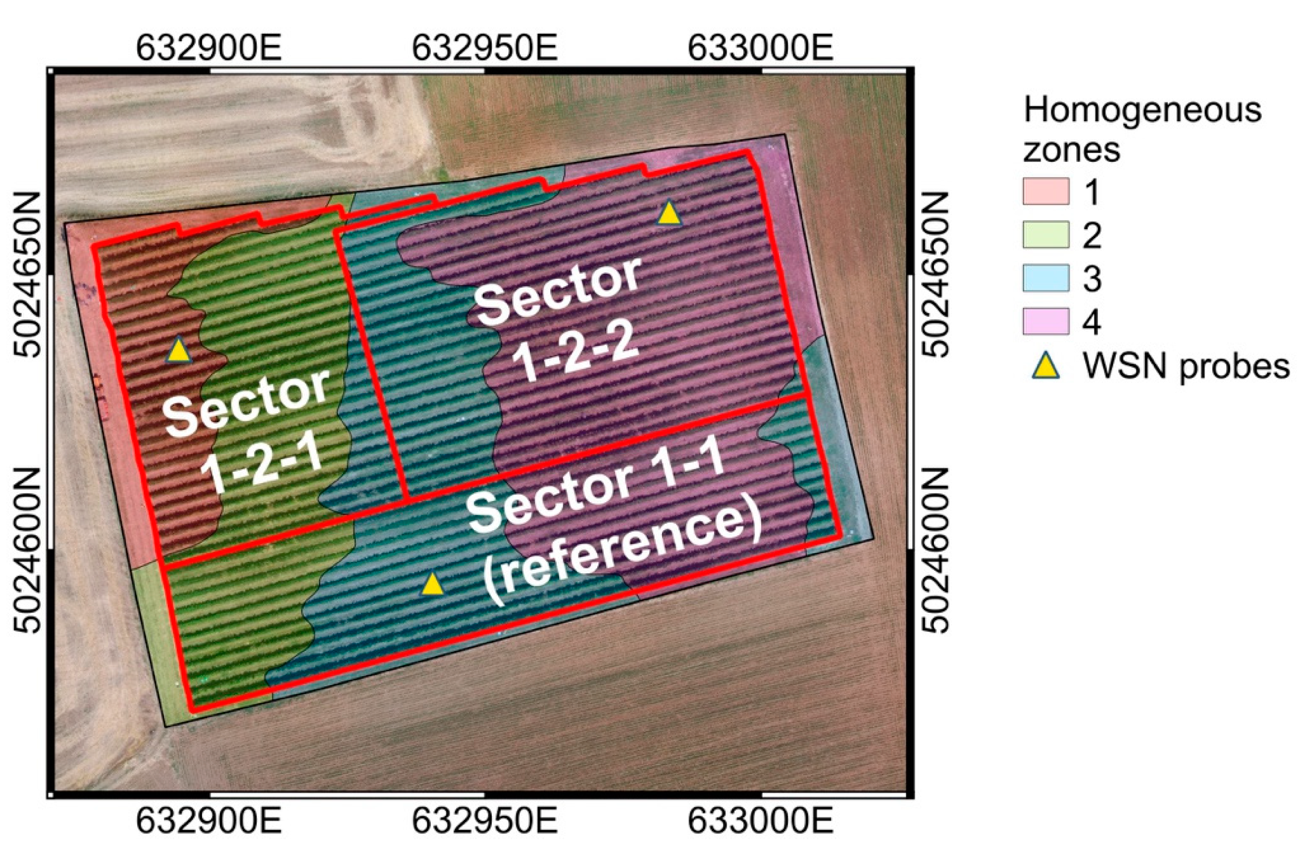
The aim of this work is to demonstrate the performance of a simple drip VRI system, designed according to the soil variability in a vineyard of 1 ha located in the Morainic Hills region south of the Garda Lake (Lombardy, Italy), in reducing irrigation water use while maintaining product yield and quality. Through the mapping of the soil electrical conductivity (EC), different management zones were identified and a drip VRI system was designed. The drip VRI system was characterized by three sectors: two sectors supplied water to different MZs, while the third sector was used to illustrate the ‘reference irrigation management’. Irrigation in the first two sectors was managed firstly according to the different crop irrigation requirements estimated considering the site-specific soil hydraulic properties, and successively on the basis of data acquired by soil moisture probes installed in each sector. Water saving and product quality and quantity were assessed by comparing results for the sectors adopting the VRI management with those of the ‘reference’ sector.

2. Materials and Methods

2.1. Pilot Site

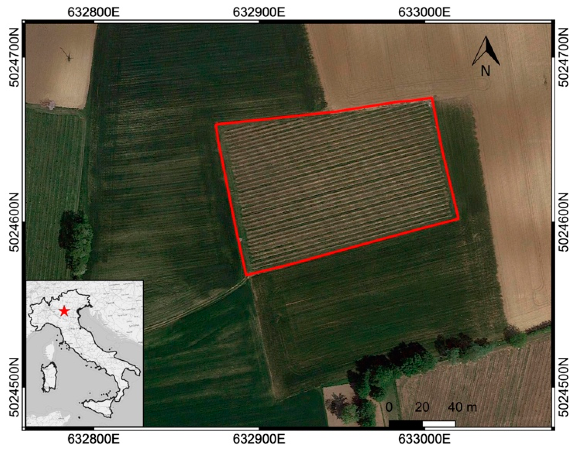
The experimental site (Figure 1) is a 1 ha vineyard located in Olfino di Monzambano, Mantua, Lombardy. The farm, entirely dedicated entirely dedicated to the production of wine grapes, is located in the heart of the Morainic Hills region, not far from Lake Garda.
The vineyard is almost flat and located at an altitude of about 88 m a.s.l. The grapevine variety is Chardonnay, cultivated with a Guyot training system in rows oriented along the east–west axis, with a distance of plants on the row of 0.8 m and a distance between the rows of 2.4 m. The plant cover fraction in the phase of maximum development of the canopy was estimated to be about 25%. The soil, both under the rows and between the rows, is grass-covered with periodic mowing to regulate the excessive development of vegetation.
In previous years, irrigation was supplied only in emergency situations through a hose-reel (a permanent drip irrigation system was not present).

2.2. Soil Variability Detection and Soil Hydrological Characterization

The first step in the soil survey was the soil variability detection. The knowledge of the within-field variability is essential in precision agriculture applications to allow management with differentiated agronomic interventions, including irrigation [24].
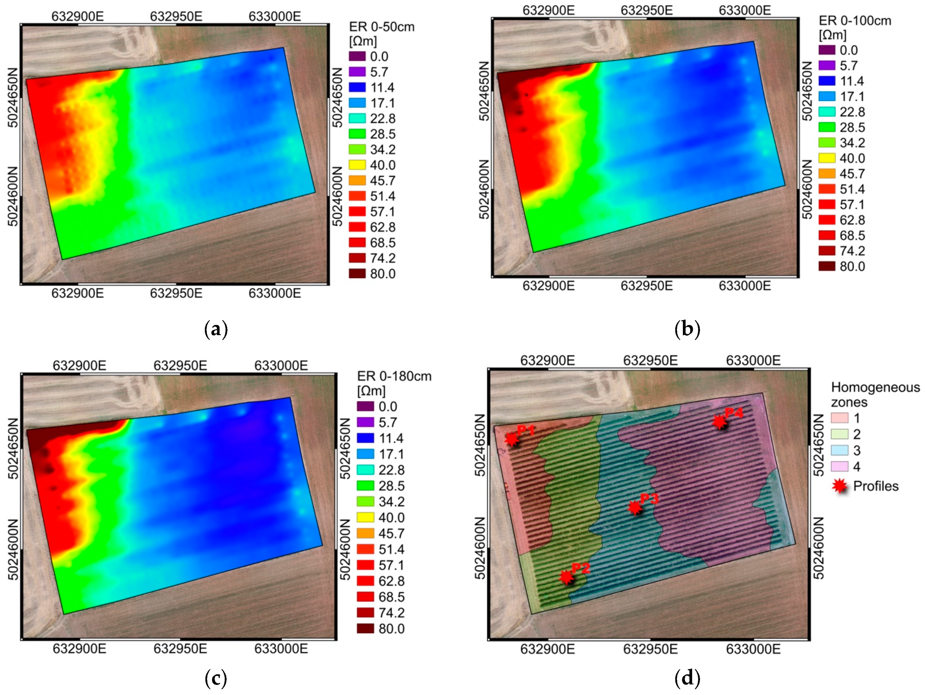
A soil survey with proximal sensing technologies was conducted in the vineyard in December 2017. An electro-magnetic induction (EMI) sensor (CMD Mini-Explorer, by GF Instruments, Czech Republic) pulled by a quad-bike was used to measure the electrical resistivity (ER) of the soil (the survey was carried out by SO.IN.G Strutture e Ambiente S.r.l.). The quad-bike, equipped with a GPS, acquired data by proceeding along parallel lines between the rows of the vineyard. CMD Mini-Explorer, which is a multi-coil EMI sensor, acquires ER measurements corresponding to the following three depths of agronomic interest: 0–50 cm, 0–100 cm and 0–180 cm.
Measured ER values were interpolated to obtain three maps which were analyzed using statistical techniques to delineate homogeneous management zones (MZ) within the field. A pedological profile was opened in each MZ to detect and analyze the main characteristics of the different soil types. For each profile, disturbed and undisturbed samples were taken from the different soil horizons, and the textural properties, the content of organic matter and many other parameters of interest were determined in the laboratory on two replicates. For each undisturbed sample, the volumetric water content at field capacity (FC) and wilting point (WP) were determined. For each soil horizon, total available water content (TAW, [25]) was calculated as the difference between FC and WP. Finally, for each MZ, the TAW in the rooting zone (assumed having a depth of 150 cm) was calculated weighting the TAW values found for each horizon by their depth.

2.3. Vineyard Irrigation Requirements

The estimation of crop water requirements is an indispensable step to design an irrigation system, as well as to define optimal irrigation depths and turns to be adopted for the irrigation management [26,27]. The irrigation requirement of a crop is defined as the quantity of water required to maintain the maximum evapotranspiration rate under optimal agricultural, water and development conditions, also taking into account soil moisture already present in the soil at the beginning of the growing season and rainfall [28]. The ‘single crop coefficient’ approach proposed in the Paper FAO-56 [
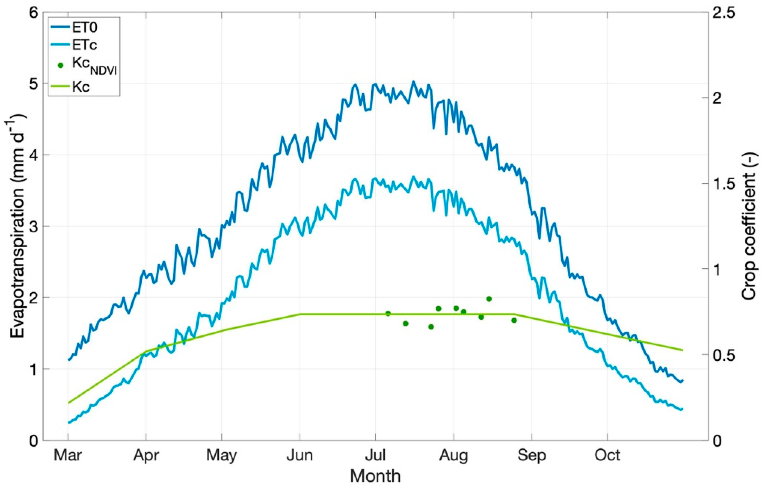
25] is one of the most used methodologies to estimate the maximum crop evapotranspiration rate. According to this method, evapotranspiration under optimal water availability conditions (ETc) is calculated by multiplying the evapotranspiration of a reference herbaceous crop (ETo) by a crop coefficient (Kc) which summarizes the different crop characteristics of the specific crop compared to the reference grass [25].

2.3.1. Agrometeorological Data and Estimation of the Reference Evapotranspiration

ETo was calculated at a daily step using the FAO Penman–Monteith equation [
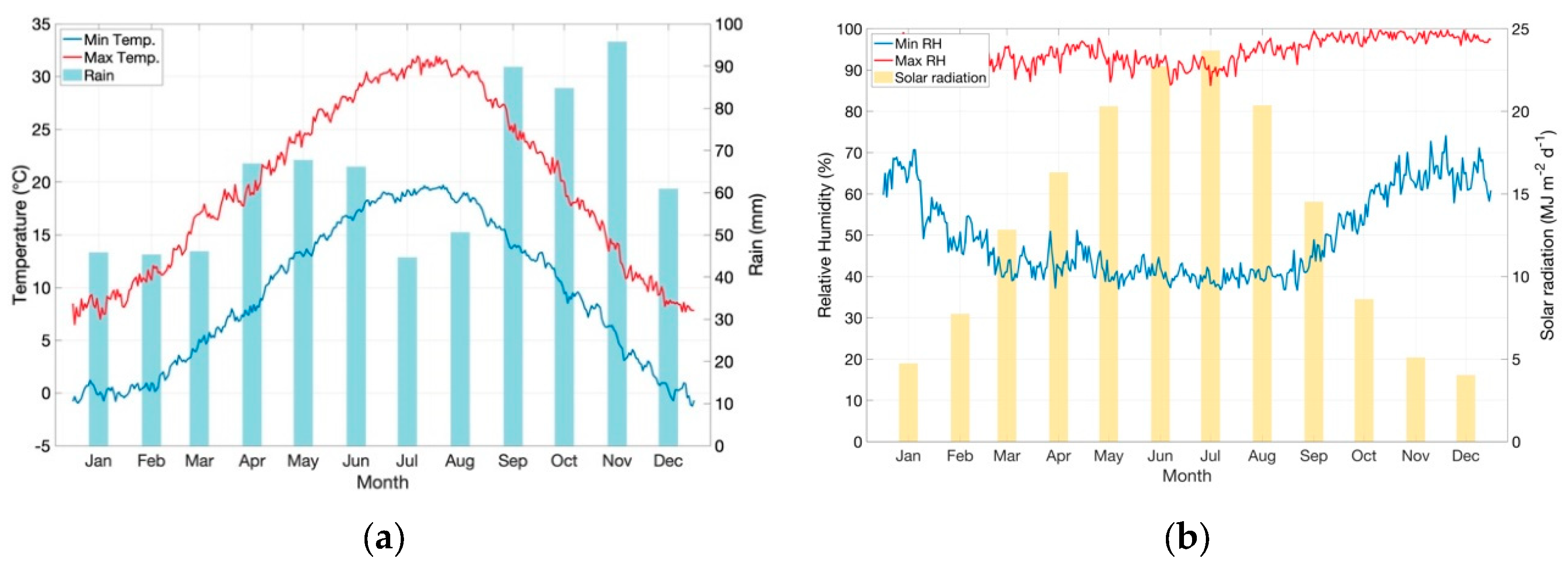
25], based on agro-meteorological data recorded at the ARPA (Regional Environmental Protection Agency) agro-meteorological station located at Ponti sul Mincio (Lat 45.412618, Lon 10.682284), about 6.5 km away from the pilot site. In order to take into account inter-annual variability of climatic variables, the agro-meteorological data from the last 25 years (1993–2017) were used to estimate ETo; finally, ETo values obtained for the 25 year series were averaged in order to obtain a mean daily value for the period March–September.
Daily mean values of maximum and minimum air temperature, together with the mean monthly cumulative precipitation values are shown in Figure 2a, while in Figure 2b the patterns of the mean values of solar radiation and air humidity are reported.

2.3.2. Crop Coefficient and Phenological Phases

The need to adopt site-specific Kc curves representative of the local conditions is essential for an accurate estimation of crop water requirements, especially in the case of tree crops which may have different planting geometries and grass cover conditions. Indeed, as pointed out by several authors [26,27,28], the use of tabulated Kc values in the case of vineyards is made poorly effective by the great heterogeneity in the vineyard characteristics and management, which may depend on many site-specific factors: cultivar type, row orientation, canopy shape and structure, training system, planting distance, ground management along the row and between the rows.
For this reason, several authors suggest, when possible, the use of locally measured or estimated phenological stage lengths and Kc values. Different approaches and devices could be used to directly or indirectly estimate Kc, such as lysimeters, hydrological balance models, micro-meteorological stations (Bowen-ratio or Eddy-covariance), and remote sensing applications [26,28,29]. In [26], linear empirical relationships are presented between the dual-crop coefficient Kcb [25] of grapevine and two spectral indices, NDVI and SAVI, showing a good correlation between Kcb and both the spectral indices.
The relationship developed in [26] between Kcb and the NDVI is the following:
Kcb = 1.44 · NDVI 0.1 .
The NDVI is one of the most widely used indices for agricultural applications and, in general, for vegetation monitoring [28]. In vineyards, NDVI has been shown to be well correlated with the evapotranspirative rate and the plant water status [30], and to maintain a rather stable field variability pattern from one year to another, being influenced by factors of the soil–crop system which are fairly stable over time, such as soil texture and soil water availability [20].
This index is calculated as:
NDVI = ( ρ NIR ρ Red ) / ( ρ NIR + ρ Red )
where ρ is the canopy reflectance value for the NIR and the Red spectral bands.
In this study, Equation (1) was used to obtain a Kc curve representative of the local conditions of the vineyard. The adopted methodology is described hereafter. Sentinel-2 (ESA; spatial resolution, 10 m; temporal resolution, 5 days) multispectral images of the vineyard area were downloaded and analyzed to calculate the NDVI index. NDVI values were computed in different points of the vineyard, excluding pixels close to the field’s edges to avoid ‘border effects’. Values calculated for the different points were averaged to obtain a single value for each date. Finally, values found for the different dates were averaged to obtain monthly values. Only images of July and August 2017 were analyzed, since in these months grapevine reaches its maximum development, and the spectral response of grass is thus expected to be lower. This was supposed to minimize errors due to the 10-m pixel of the Sentinel-2 imagery, including both crop and inter-row grass. The Kcb values calculated according to Equation (1) were then converted to Kc values by increasing them by a constant factor of 0.05, as suggested in FAO-56 for Kcmid (Kc at the maximum canopy development stage).
A literature research was carried out to find suitable values for Kc at the initial and final stages of the development cycle (Kcini and Kcend), as well as to compare the Kcmid obtained in this study with values obtained in other studies. Due to the lack of specific studies carried out on cv. Chardonnay, the monthly values of Kc reported in [31] were considered and used as a reference. Even if values reported were not specific for the Chardonnay variety, in the central part of the season they showed to be very similar to those obtained from the application of Equation (1). Kc values found in [31] were then rescaled by assigning the maximum value obtained through Equation (1) to the central months and recalculating the values for the other months by multiplying them by the ratio between the Kcmid value obtained in this study and the correspondent literature value.
The maps produced in the iPhen project [32] for the years 2015, 2016 and 2017 were used to estimate the length of the phenological phases of the vineyard. These maps report, at a weekly time step, phenological stages observed for the grapevine Chardonnay variety in different areas of Italy. Starting dates of the main phenological phases were extracted from these maps, and the average value over three years was used as the starting date of each phenological phase in this study.
To simplify the irrigation management, the whole irrigation season was divided into four periods depending on the grapevine main phenological stages and on the different sensitivity to water stress of plants in each stage. This type of approach, consisting in subdividing the crop cycle into a few but easily distinguishable ‘irrigation phases’ is commonly used and, for instance, suggested in the ARSIA (Italian Regional Agency for Development and Innovation in the Agricultural and Forestry Sectors) worksheets [33] implemented for several herbaceous and arboreal crops in central Italy (Tuscany). In this study, the following subdivision in ‘irrigation phases’ is adopted: budding and vegetative development (phase 1), flowering and fruit setting (phase 2), veraison (phase 3), and maturation until harvest (phase 4) [31].

2.4. Irrigation Requirement Estimation

Usually, irrigation requirement is computed by subtracting the contribution of rainfall to ETc. In this study, considering the great inter-annual variability that characterizes rainfall amounts, ETc was assumed to be a ‘safer’ estimate of the irrigation requirement. In particular, the irrigation requirement with a probability of non-exceedance of 75% (Fi, mm d−1) was calculated as follows:
F i = F im + z σ
where Fim is the mean daily ETc of the phase, σ is the standard deviation of the daily ETc of the phase, and z is the value corresponding to the 75th percentile in a standard normal distribution (i.e., 0.674).
Fi represents the net irrigation needs; to obtain the gross irrigation requirements (Fil, mm d−1), which represents the water amount that should be provided to the field through irrigation, the theoretical efficiency of the irrigation system (Eadac) must be considered. Eadac for a drip irrigation system can be considered close to 95%. Fil is finally obtained dividing Fi by Eadac:
F il = F i / E adac .
For each phase, the irrigation requirement estimate was used to define optimal irrigation depths and turns, as illustrated in the next Section 2.5.

2.5. Irrigation System Design, Preliminary Irrigation Scheduling and Irrigation Management

A variable-rate drip irrigation (VRDI) system was designed considering the irrigation requirements of the crop, the spatial pattern of management zones (i.e., homogeneous zones with respect to the soil properties, MZs), and the hydrological characteristics of the different soil profiles measured in the laboratory. The first important point to be considered in designing a VRDI concerns the number and layout of sectors with respect to the identified MZs. A VRI system should, ideally, be able to follow as much as possible the spatial variability detected in the field, in order to ensure a distribution of water well in accordance with the identified crop irrigation needs [22]. This need to have a high level of spatial differentiation in the irrigation supply collides with the complexity and the cost of the technical solution to be implemented: the more field zones there are to be managed, the more irrigation sectors with different characteristics and operating independently of each other there must be [19]. To pursue an economically viable solution, it is however necessary to reach a compromise between the spatial variability detected in the field and the number of homogeneous zones that can be managed.
In this study, to design the VRDI system, a simplified pattern of MZs was created by merging the MZs with similar soil properties, in such a way to identify a limited number of main MZs. A VRDI characterized by as many sectors as the main MZs, each one controlled by an independent electrovalve, was designed and realized. Drip lines selected for the sectors were different in terms of spacing between drippers and dripper flow rates, based on the type of soil within the MZ. An additional sector designed to include as much as possible the soil variability within the vineyard was established as the ‘reference sector’; the most common drip lines used for drip irrigation in vineyards were installed in this sector.
An irrigation prescription map (IPM) was obtained on the basis of the TAW value computed for each MZ. A preliminary irrigation scheduling for each crop phenological stage and each sector was obtained based on TAW values and crop water requirements. The irrigation scheduling concerned irrigation turn periods, duration of the irrigation event and irrigation depths for each sector.
The gross maximum water depth which can be provided by irrigation, hal max (mm), is a function of TAW and it was calculated as follows:
h al   max = Z r · p · TAW · S b E adac ,
where TAW (m3 m−3); p (–) is the fractional depletion of TAW, set to 0.45 for grapevine as suggested in [25]; Zr (mm) is the rooting depth, set to 1500 mm; Sb (–) is the wetted surface, set to 25%.
The theoretical irrigation turn period, Tg (days), was calculated for each growth stage dividing hal max by the daily average value of the irrigation requirement, Fil (mm d−1), calculated for the same period:
T g = h al   max F il .
To simplify the irrigation management, the value of Tg calculated according to Equation (6) can be rounded to the nearest lower integer Tgi, so that the actual gross water depth, hal (mm), provided in each irrigation becomes:
h al = T gi · F il .
Finally, the duration of the irrigation event for each growth stage, da (hours), was calculated as:
d a = h al I a ,
where Ia (mm h−1) is the irrigation intensity within each sector, depending on the characteristics of the VRDI system (dripper flow rate, dripper distance and plant row distance in the vineyard).
The theoretical irrigation turns and duration (Equations (6) and (8)), and subsequently the actual irrigation depth provided in each irrigation event, for this study needed to be adapted to the constraints imposed by the Garda–Chiese Irrigation Consortium (GCIC), which manages the irrigation service in the area including the pilot farm. At the beginning of the season, the irrigation service provided by GCIC to the farm was based on an irrigation turn of 8 days for a duration of 15 h. However, this constraint proved to be too restrictive for the successful implementation of the study. Thus, GCIC started to deliver irrigation water to the farm every 4 days for 7 h. Consequently, the irrigation management of the vineyard was modified to take into account of this new constraint.
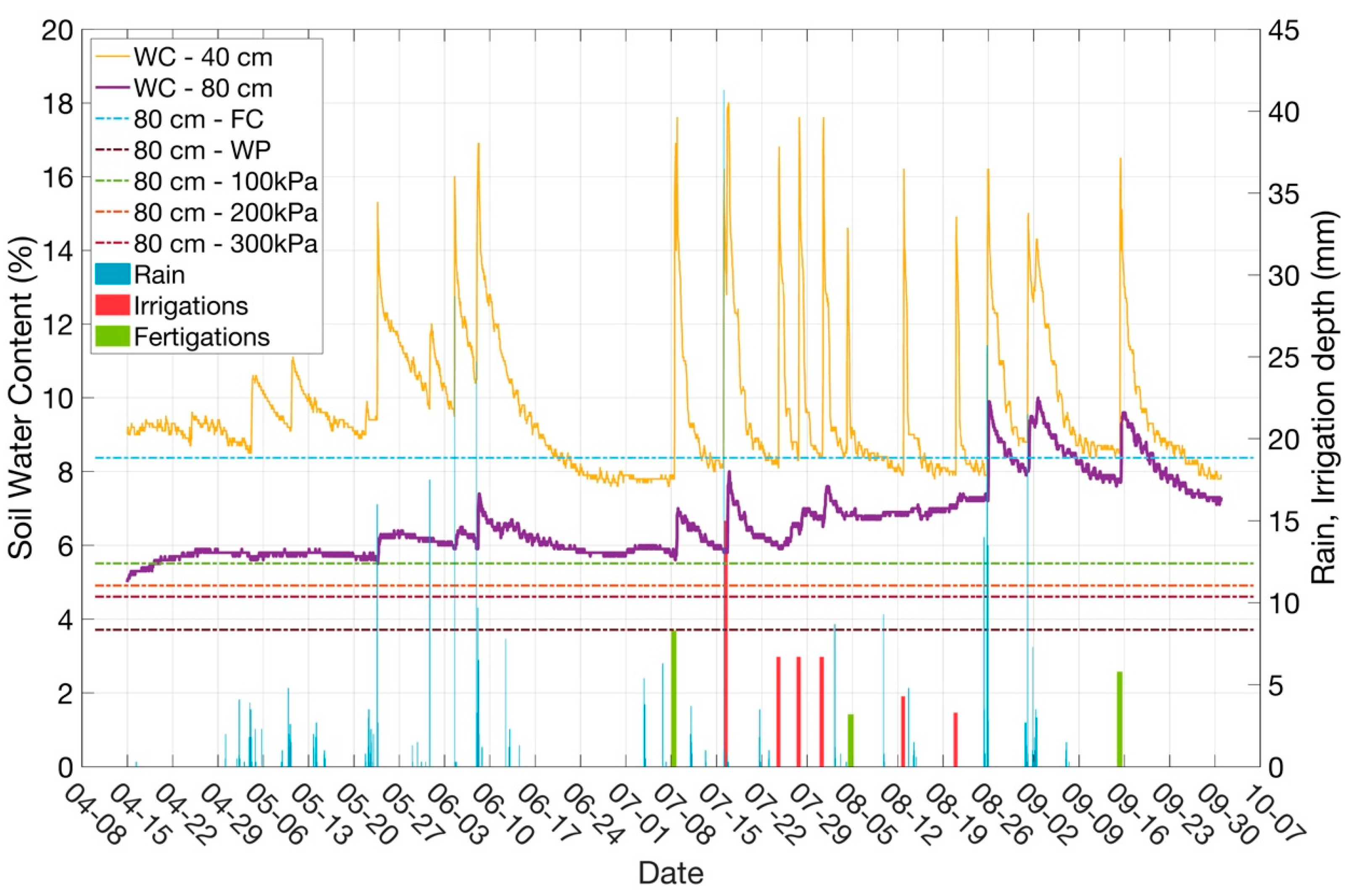
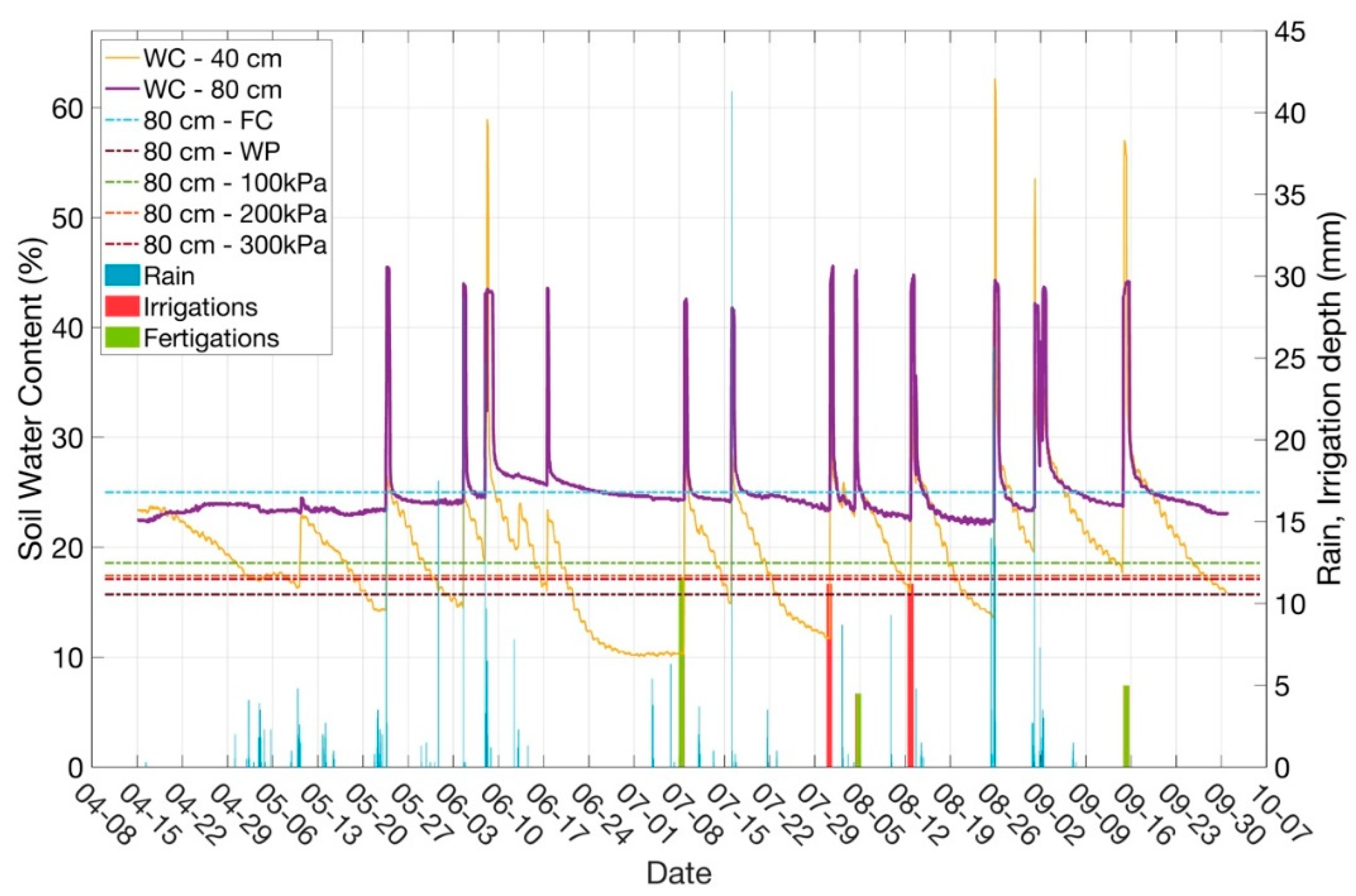
Moreover, the preliminary irrigation scheduling defined using Equations (5)–(8) was modified during the irrigation season considering the actual soil moisture dynamics, measured by means of a wireless soil water content sensor network (WSN) installed within the vineyard. In particular, the soil water content sensors were installed at two depths (40 and 80 cm) in one point for each irrigation sector. The irrigation was provided in order to avoid the decrease of the soil water content at 80 cm under a fixed threshold, below which crop would start suffering for water shortage. Examples of irrigation thresholds for grapevine are reported in [34], where a water potential value of −150 kPa measured at 60 cm depth is proposed, or in [35], in which a threshold of −120 kPa is instead suggested. For grapevine, especially in certain phenological phases, controlled water stress conditions can be accepted or even set. In this work, three different thresholds were adopted, depending on the phenological stage. In particular: −100 kPa for the first stages (until fruit set and growth), −200 kPa for the veraison stage, and −300 kPa during the maturation phase.
An additional point of the WSN was located within the ‘reference sector’, even if the irrigation in this sector was supplied according to farmer’s decisions, and soil water content sensors were used uniquely to monitor the soil moisture behavior. Finally, an agro-meteorological station was installed during the study and used to cross-check the soil water content sensor response.

2.6. Product Quantity and Quality and Irrigation Water Productivity

At harvest (27 August 2018), the bunches on vines were counted and the total yield per vine was recorded in six biological repetitions for each sector. Berry fresh weight was measured on 50 berries per plant. Bunches from median shoots were pressed to obtain the must for each repetition and the fermentation was prevented adding NaN3 at 0.2‰ to each sample. Sugar content (°Brix) of must was determined by using the refractometer RBO-Optech, Germany. Titratable acidity (g L−1) and pH were measured with the titrator CRISON Compact. All data were analyzed using Microsoft Office Excel and IBM SPSS Statistics 24. Statistical significance was assessed at p ≤ 0.05 for analysis of variance (one-way ANOVA test) and post-hoc comparisons (Duncan test).
Finally, to assess the water use efficiency for each sector, the irrigation water productivity (IWP) index was calculated as the ratio of the yield (kg) to the volume of irrigation water (m3) applied. Since the total yield per sector was not measured, it was estimated by dividing the sector area by the vines spacing, thus obtaining the average number of vines in each sector and multiplying the number of plants by the average production per vine.

3. Results and Discussion

3.1. Soil Variability Detection and Soil Hydrological Characterization

The results obtained from the interpolation of the ER data for the three soil depths are shown in Figure 3a–c. Four homogeneous soil types were identified through cluster analysis of ER data, allowing to hypothesize a similar pattern of homogeneity in the hydrological characteristics of the soils. The four homogeneous zones are shown in Figure 3d, together with the points where the pedological profiles were opened (P1–P4).
In Table 1 the results of the laboratory analysis for the investigated soil profiles are reported. For each horizon the depth of the upper and lower limits, the percentage of sand, silt and clay and the values of FC, WP and TAW are reported. Texture classes were determined according to the USDA classification. The TAW values were obtained as a weighted average of the values measured for the different horizons, considering a maximum rooting depth of 150 cm.
From the pedological survey all the four soils were assumed to derive from fluvioglacial or glacial deposits; they appear well drained, with a high (P3) or moderate (P1, P2 and P4) water capacity and average organic carbon. According to the USDA soil taxonomy, P1, P2 and P3 were classified as Typic Ustorthents fine, carbonatic, mesic, semiactive; P1 and P2 showed also to be rich in skeleton in the upper 100 cm. P4 was classified as Typic Haplustalfs fine, carbonatic, mesic, semiactive.
The P1 soil, which showed a higher ER than the others, was found to have the highest skeleton and sand content; the average values of ER progressively tended to decrease in the P2–P4 profiles. Such a variability pattern may be due to a gradual increase in the water capacity of soils, moving from P1 to P4, therefore following an east–west gradient. As often reported in the literature, indeed, a decrease in ER corresponded to an increase in soil water content [36,37].

3.2. ET0, ETc and Crop Irrigation Requirements Estimation

The average daily ETo series calculated by applying the Penman–Monteith equation to the agrometeorological data of the last 25 years (Section 2.3.1) is shown in Figure 4. ETo (dark blue line) shows a typical pattern with an almost linear growth from March to June and a peak between the end of June and the end of July, with values between 4.6 and 5 mm day−1, followed by a constant decrease until the end of the irrigation season. Relevant is the fact that the peak of ETo corresponds to the month in which the lowest value of average cumulated rain is recorded (Figure 2a). The cumulate ETo value for the period March–September is 725 mm. In [31] the maximum value of Kc (Kcmid) for the months of June, July and August was 0.68. The average value of Kc obtained from the application of Kc–NDVI relationship for the months of July and August was instead equal to 0.735 (Kc values obtained from satellite data are reported as KcNDVI in Figure 4). The two values were used to calculate a ratio (1.08) then used to modify Kc values reported in [31] to obtain the Kc curve reported in light green in Figure 4.
Starting from the ETo and the Kc curve, the crop evapotranspiration under optimal conditions, ETC, was calculated. As for the ETo, also for ETC (light blue in Figure 4) it is possible to detect an increasing and a decreasing phase, and a peak between late June and July, with maximum values of 3.5 mm day−1. Such a trend in the vine ETC is similar to what reported for this crop in [26,38]. The cumulated ETC for the period March–September is 492 mm, in line with values reported by [26,38,39] for grapevine, although in environments characterized by less humid climates.
Table 2 shows the four phases in which the vineyard growing period was divided, the starting and ending dates estimated by the iPhen project maps, and the average Kc values calculated. Moreover, in the last four columns, the mean and standard deviation of ETC for each stage, and net and gross irrigation requirements are also illustrated.

3.3. Design of the VRDI System

To design the VRDI system in the studied vineyard, the four MZs (Figure 3d) were grouped, and two main MZs were identified. The first MZ included the coarsest soils (described by soil profiles P1 and P2), while the second one included the heaviest soils (described by soil profiles P3 and P4). The average TAW value of soils included in each main MZ was used for the IPM. The designed VRDI system had three irrigation sectors, two of which corresponded to the main MZs (Sector 1-2-1 and Sector 1-2-2, characterized by TAW values of 7.5% and 12%, respectively) and were managed in a different way on the basis of the soil hydrological properties. The third sector (Sector 1-1) was designed to incorporate as much soil variability as possible (P2, P3 and P4), to represent the average conditions of the field, and was managed on the basis of the farmer’s experience (‘reference sector’). The three sectors are shown in Figure 5.
Dripper spacing and flow rate were different for Sectors 1-2-1 and 1-2-2, since drippers were selected among those available on the market on the basis of the soil properties within each MZ. In particular, since in coarse soils flow is prevalently vertical, low flow rates and short spacing are usually suggested to avoid percolation; on the contrary, heavy soils are characterized by both vertical and lateral water diffusion, and higher flow rates and larger spacing may be adopted. For the third sector, the most common drippers used in drip irrigation of vineyards were selected. The main features of the irrigation material installed in the three sectors are summarized in Table 3.

3.4. Irrigation Scheduling and Management

3.4.1. Irrigation Turns and Water Depths

The first two sectors of the VRDI system had a different irrigation management (irrigation turn, height and duration) based on the vineyard irrigation requirements and the dripper characteristics in each sector. The gross maximum water depth (mm), the irrigation turn (days), the duration of the irrigation event (hours) and the actual gross water depth provided in each irrigation event (mm) calculated for Sectors 1-2-1 and 1-2-2 are reported in Table 4; values modified by taking into account the constraints imposed by the GCIC (as explained in Section 2.5) are reported in brackets. These values were used as an initial reference for the management of the VRDI system.
Due to a long rainy period in June 2018, the irrigation was actually managed only from the beginning of July until the beginning of September. During this period, the irrigation frequency, duration and depth reported in Table 4 were optimized depending on the evolution of the soil water content measured by the WNS (whose position in shown in Figure 5), as better explained in the next section.

3.4.2. Soil Water Content and Irrigation Scheduling

The irrigation management was fine-tuned during the irrigation season by taking into account only the soil water content probe measuring at a depth of 80 cm, since this depth was considered to be more representative of the actual water availability in the root zone. In particular, irrigation was provided in order to prevent the soil water content at 80 cm from falling below fixed thresholds, below which crop would start suffering for water shortage. The following three different thresholds, depending on the phenological stage, were adopted (expressed in terms of soil water potential): −100 kPa for stages 1 and 2 (until fruit set and growth), −200 kPa for veraison stage (stage 3) and −300 kPa during the maturation phase (stage 4). Moreover, three fertigation events were provided at the beginning, half and end of the irrigation season. Fertigations were planned by an agronomist who indicated the periods when fertigation was advised; fertigations were provided independently of the soil water content, on the first day of water availability according to the turns imposed by GCIC.
To compare values detected by the probes with thresholds, the latter were converted to volumetric water contents by applying the soil water retention curve measured in the laboratory for the soil horizon including the depth of 80 cm. In Figure 6 and Figure 7 the soil water content measured by the WSN probes from 15th April to the end of September are reported for Sectors 1-2-1 and 1-2-2, respectively; values measured for both depths are reported although all the thresholds refer only to 80 cm depth (purple bold line). In the charts also rainfall and irrigation events are illustrated.
The actual irrigation events, their duration (hours) and water depth (mm) are reported in Table 5. The first noticeable difference between actual and reference irrigation schedules is that actual irrigation events were concentrated in July and August, with the exception of a single intervention in September (for fertigation). The first months of the agricultural season of 2018 were, indeed, characterized by intense rainfall, which delayed the start of irrigation operations. In the Sector 1-2-1, characterized by coarse soils and a low TAW value, the frequency and number of irrigations were higher than in sector 1-2-2, with finer soils and a higher TAW, but the irrigation events were shorter, providing lower irrigation depths; this decision was taken according to the soil characteristics: with the TAW value in Sector 1-2-1 being rather low, longer irrigations would have resulted in high losses due to percolation. The variability in irrigation depths along the season for each sector was due to different reasons: in particular, some irrigation events, with a lower irrigation depth, were for fertigation.
Focusing on the 80 cm water content, on which the irrigation management was based, it can be observed that in both sectors the water content never fell below the threshold corresponding to −100 kPa soil water potential, principally due to rainfall, often occurring shortly after an irrigation event. This suggests that the grapevine did not experience any water stress during the entire season.

3.5. Water Consumption, Crop Yield and Irrigation Water Productivity

An overall assessment of water use in the three sectors of the vineyard is reported in Table 6. For each sector the supplied water volume (m3), the unit volume (m3 ha−1) and the difference with the reference sector (%) are reported. The unit irrigation volume was calculated by dividing the total volume supplied to each sector by its area. The sum of water consumption in the two sectors 1-2-1 and 1-2-2 was also considered in order to allow the comparison between the whole VRDI system results and the reference sector.
The VRI management, in combination with a careful assessment of crop irrigation needs and soil moisture trends, led to a −39% reduction of water compared to control for sector 1-2-2, while in sector 1-2-1 a slightly higher unit volume was applied (+11%). These contrasting results were due to the different soil water retention properties characterizing the two sectors. The coarse soils of sector 1-2-1, characterized by high contents of sand and in some areas also of gravel, required irrigation applications more frequently than the sector 1-2-2, characterized by fine soils. Indeed, irrigation (without considering fertigations) was provided five and two times in sectors 1-2-1 and 1-2-2, respectively. On the other hand, considering the total surface of both sectors, the VRI management globally reduced the water application. Considering both sectors, a water saving of 18% was achieved. This result is slightly higher than that achieved, for instance, in [19], where with a much more complex irrigation system a maximum saving of 17% was obtained. Since the 2018 season was rather rainy, it is not unlikely that in drier years the total volume saved could be even greater.
Since water availability is one of the factors that mostly influence the physiology of the vine, affecting the production of grapes in terms of quantity and quality [12], in Table 7 the main yield and quality parameters of grapes harvested in the different sectors are reported.
For what concerns the yield per vine (kg), the number of bunches and their average weight, and the average berry weight, there is no statistically significant difference between the VR irrigation sectors and the control. The coarse soil of sector 1-2-1 slightly affected the sugar content, which is lower than in the other sectors; the titrable acidity also shows slight differences in the three sectors (Table 7). No differences of pH were instead observed among the three sectors (Table 7).
The values of the irrigation water productivity (IWP) index found for the two managed sectors (Table 8), respectively 33 and 58 kg m−3, reflect the trend shown in Table 6 for the unit water application; for Sector 1-2-1, due to reasons already explained above, the index has a lower value with respect to the value found for the reference sector. However, when both sectors are considered together, the global IWP value is higher than that found for the reference sector (44 kg m−3).
Finally, according to the farmer’s experience, the qualitative parameters have shown a higher homogeneity on the whole vineyard than in previous years (when a fixed irrigation system was absent), allowing to avoid harvesting operations conducted in different times.

4. Conclusions

This work aimed at demonstrating the feasibility and the effectiveness of a simple VRDI system in a 1 ha vineyard located in Northern Italy during the 2018 agricultural season, as a concrete possibility of adopting on-farm precision irrigation techniques to reduce water use while having positive effects on the production.
After a preliminary soil hydrological characterization, two different main MZs were recognized and a VRDI system consisting of two sectors (plus a ‘reference sector’) was designed and realized. A soil water content wireless network (WSN) was installed. The preliminary irrigation scheduling, defined for each sector taking into account soil properties and grapevine irrigation requirements in each phenological stage, was dynamically modified during the growing season based on the soil moisture measurements. This allowed to take into account real time weather conditions (evapotranspiration demand and rainfall events).
The main result of this study is the reduction in water consumption achieved with the drip VRI management compared to the conventional drip management. If the vineyard was uniformly irrigated like the reference sector, 18% more water would have been used by the farmer. No statistically significant differences in yield and qualitative product parameters among the different sectors were found. Moreover, product qualitative parameters have shown, in general, a higher homogeneity over the vineyard than in previous years (when a fixed irrigation system was absent). The obtained results stress how the consideration of the within-field spatial variability can have a relevant role in the optimization of the irrigation management and in the improvement of product quality.
This study demonstrates how a relatively simple solution for the implementation of VRI could be designed and implemented in commercial vineyards, showing that precision irrigation techniques are ready to provide tangible results that may be of interest not only for researchers but also for farmers.

Author Contributions

Conceptualization, B.O., A.F. and L.B.; Data curation, B.O., A.M. and A.B.; Formal analysis, B.O., A.M. and D.B.; Funding acquisition, B.O., A.F. and L.B.; Investigation, B.O., A.F., A.M. and D.B.; Methodology, B.O. and A.F.; Project administration, B.O., A.F. and L.B.; Supervision, A.F. and L.B.; Visualization, A.M.; Writing—original draft, A.M.; Writing—review & editing, B.O., A.F. and A.M.

Funding

We wish to thank Regione Lombardia for funding the NUTRIPRECISO project (EU-RDP 2017), in the context of which this research was developed.

Conflicts of Interest

The authors declare no conflict of interest.

References

  1. Pachauri, R.K.; Allen, M.R.; Barros, V.R.; Broome, J.; Cramer, W.; Christ, R.; Church, J.A.; Clarke, L.; Dahe, Q.; Dasgupta, P.; et al. Climate Change 2014: Synthesis Report. Contribution of Working Groups I, II and III to the Fifth Assessment Report of the Intergovernmental Panel on Climate Change; Pachauri, R.K., Meyer, L., Eds.; IPCC: Geneva, Switzerland, 2014. [Google Scholar]
  2. Monaghan, J.M.; Daccache, A.; Vickers, L.H.; Hess, T.M.; Weatherhead, E.K.; Grove, I.G.; Knox, J.W. More ‘crop per drop’: Constraints and opportunities for precision irrigation in European agriculture. J. Sci. Food Agric. 2013, 93, 977–980. [Google Scholar] [CrossRef] [PubMed]
  3. United Nations. Transforming Our World: The 2030 Agenda for Sustainable Development. Ocean. Yearb. 2015, 30, 782–824. [Google Scholar]
  4. Haghverdi, A.; Leib, B.G.; Washington-Allen, R.A.; Ayers, P.D.; Buschermohle, M.J. Perspectives on delineating management zones for variable rate irrigation. Comput. Electron. Agric. 2015, 117, 154–167. [Google Scholar] [CrossRef]
  5. Bellvert, J.; Zarco-Tejada, P.J.; Girona, J.; Fereres, E. Mapping crop water stress index in a “Pinot-noir” vineyard: Comparing ground measurements with thermal remote sensing imagery from an unmanned aerial vehicle. Precis. Agric. 2014, 15, 361–376. [Google Scholar] [CrossRef]
  6. Whelan, B.M.; McBratney, A.B. The “null hypothesis” of precision agriculture management. Precis. Agric. 2000, 2, 265–279. [Google Scholar] [CrossRef]
  7. Matese, A.; Di Gennaro, S.F. Technology in precision viticulture: A state of the art review. Int. J. Wine Res. 2015, 7, 69–81. [Google Scholar] [CrossRef]
  8. Cordoba, M.A.; Bruno, C.I.; Costa, J.L.; Peralta, N.R.; Balzarini, M.G. Protocol for multivariate homogeneous zone delineation in precision agriculture. Biosyst. Eng. 2016, 143, 95–107. [Google Scholar] [CrossRef]
  9. Bramley, R.; Lamb, D. Making sense of vineyard variability in Australia. In Proceedings of the International Symposium on Precision Viticulture, Ninth Latin American Congr on Viticulture and Oenology; Facultad de Agronomia e Ingeneria Forestal: Santiago, Chile, 2003. [Google Scholar]
  10. Green, D.R.; Szymanowski, M. Monitoring, mapping and modelling the vine and vineyard: Collecting, characterising and analysing spatio-temporal data in a small vineyard. In Proceedings of the IXth International Terroirs Congress, Dijon/Rheims, France, 25–29 June 2012. [Google Scholar]
  11. Bonfante, A.; Basile, A.; Langella, G.; Manna, P.; Terribile, F. A physically oriented approach to analysis and mapping of terroirs. GEODERMA 2011, 167–68, 103–117. [Google Scholar] [CrossRef]
  12. Castellarin, S.D.; Bucchetti, B.; Falginella, L.; Peterlunger, E. Influenza del deficit idrico sulla qualità delle uve: Aspetti fisiologici e molecolari. Italus Hortus 2011, 18, 63–79. [Google Scholar]
  13. Girona, J.; Mata, M.; del Campo, J.; Arbones, A.; Bartra, E.; Marsal, J. The use of midday leaf water potential for scheduling deficit irrigation in vineyards. Irrig. Sci. 2006, 24, 115–127. [Google Scholar] [CrossRef]
  14. Arrizabalaga, M.; Morales, F.; Oyarzun, M.; Delrot, S.; Gomes, E.; Irigoyen, J.J.; Hilbert, G.; Pascual, I. Tempranillo clones differ in the response of berry sugar and anthocyanin accumulation to elevated temperature. Plant Sci. 2018, 267, 74–83. [Google Scholar] [CrossRef] [PubMed]
  15. Costa, J.M.; Vaz, M.; Escalona, J.; Egipto, R.; Lopes, C.; Medrano, H.; Chaves, M.M. Modern viticulture in southern Europe: Vulnerabilities and strategies for adaptation to water scarcity. Agric. Water Manag. 2016, 164, 5–18. [Google Scholar] [CrossRef]
  16. Fader, M.; Shi, S.; von Bloh, W.; Bondeau, A.; Cramer, W. Mediterranean irrigation under climate change: More efficient irrigation needed to compensate for increases in irrigation water requirements. Hydrol. Earth Syst. Sci. 2016, 20, 953–973. [Google Scholar] [CrossRef]
  17. Bellvert, J.; Zarco-Tejada, P.J.; Marsal, J.; Girona, J.; Gonzalez-Dugo, V.; Fereres, E. Vineyard irrigation scheduling based on airborne thermal imagery and water potential thresholds. Aust. J. Grape Wine Res. 2016, 22, 307–315. [Google Scholar] [CrossRef]
  18. McClymont, L.; Goodwin, I.; Mazza, M.; Baker, N.; Lanyon, D.M.; Zerihun, A.; Chandra, S.; Downey, M.O. Effect of site-specific irrigation management on grapevine yield and fruit quality attributes. Irrig. Sci. 2012, 30, 461–470. [Google Scholar] [CrossRef]
  19. Sanchez, L.A.; Sams, B.; Alsina, M.M.; Hinds, N.; Klein, L.J.; Dokoozlian, N. Improving vineyard water use efficiency and yield with variable rate irrigation in California. Adv. Anim. Biosci. 2017, 8, 574–577. [Google Scholar] [CrossRef]
  20. Acevedo-Opazo, C.; Tisseyre, B.; Guillaume, S.; Ojeda, H. The potential of high spatial resolution information to define within-vineyard zones related to vine water status. Precis. Agric. 2008, 9, 285–302. [Google Scholar] [CrossRef] [Green Version]
  21. Martínez, A.; Gomez-Miguel, V.D. Vegetation index cartography as a methodology complement to the terroir zoning for its use in precision viticulture. OENO One 2017, 51, 289. [Google Scholar] [CrossRef]
  22. McClymont, L.; Goodwin, I.; Whitfield, D.M.; O’Connell, M.G. Effects of within-block canopy cover variability on water use efficiency of grapevines in the Sunraysia irrigation region, Australia. Agric. Water Manag. 2019, 211, 10–15. [Google Scholar] [CrossRef]
  23. Hedley, C.B.; Bradbury, S.; Ekanayake, J.; Yule, I.J.; Carrick, S. Spatial irrigation scheduling for variable rate irrigation. Proc. N. Z. Grassl. Assoc. 2010, 72, 97–101. [Google Scholar]
  24. Doolittle, J.A.; Brevik, E.C. The use of electromagnetic induction techniques in soils studies. Geoderma 2014, 223, 33–45. [Google Scholar] [CrossRef]
  25. Allen, R.G.; Pereira, L.S.; Raes, D.; Smith, M. Crop Evapotranspiration—Guidelines for Computing Crop Water Requirements—FAO Irrigation and Drainage Paper 56; Food and Agriculture Organization of the United Nations: Rome, Italy, 1998. [Google Scholar]
  26. Campos, I.; Neale, C.M.U.; Calera, A.; Balbontin, C.; Gonzalez-Piqueras, J. Assessing satellite-based basal crop coefficients for irrigated grapes (Vitis vinifera L). Agric. Water Manag. 2010, 98, 45–54. [Google Scholar] [CrossRef]
  27. Girona, J.; del Campo, J.; Mata, M.; Lopez, G.; Marsal, J. A comparative study of apple and pear tree water consumption measured with two weighing lysimeters. Irrig. Sci. 2011, 29, 55–63. [Google Scholar] [CrossRef]
  28. Glenn, E.P.; Neale, C.M.U.; Hunsaker, D.J.; Nagler, P.L. Vegetation index-based crop coefficients to estimate evapotranspiration by remote sensing in agricultural and natural ecosystems. Hydrol. Process. 2011, 25, 4050–4062. [Google Scholar] [CrossRef]
  29. Steduto, P.; Hsiao, T.C.; Fereres, E.; Raes, D. Crop Yield Response to Water; FAO Irrigation and Drainage Paper; Food and Agriculture Organization of the United Nations: Rome, Italy, 2012; ISBN 978-92-5-107274-5. [Google Scholar]
  30. Cancela, J.J.; Fandino, M.; Rey, B.J.; Dafonte, J.; Gonzalez, X.P. Discrimination of irrigation water management effects in pergola trellis system vineyards using a vegetation and soil index. Agric. Water Manag. 2017, 183, 70–77. [Google Scholar] [CrossRef]
  31. Ragazzi, F.; Zamarchi, P. I suoli Del Lison-Pramaggiore. In Zonazione Della DOC Lison Pramaggiore—Manuale d’uso del Territorio; Veneto Agricoltura: Legnaro, Italy, 2008. [Google Scholar]
  32. iPhen—Italian Phenological Network. Available online: http://iphen.entecra.it/cma/iphen/ (accessed on 20 July 2019).
  33. Giannini, A.; Bagnoni, V. Schede di Tecnica Irrigua per L’agricoltura Toscana; ARSIA: Firenze, Italy, 2000; ISBN 978-88-8295-015-6. [Google Scholar]
  34. Holler, M.; Vineyards, C. High-density, multiple depth, wireless soil moisture tension measurements for irrigation management. Am. J. Enol. Vitic. 2008, 59, 339A. [Google Scholar]
  35. Centeno, A.; Baeza, P.; Ramon Lissarrague, J. Relationship between Soil and Plant Water Status in Wine Grapes under Various Water Deficit Regimes. Horttechnology 2010, 20, 585–593. [Google Scholar] [CrossRef] [Green Version]
  36. Ozcep, F.; Tezel, O.; Asci, M. Correlation between electrical resistivity and soil-water content: Istanbul and Golcuk. Int. J. Phys. Sci. 2009, 4, 362–365. [Google Scholar]
  37. Samouelian, A.; Cousin, I.; Tabbagh, A.; Bruand, A.; Richard, G. Electrical resistivity survey in soil science: A review. Soil Tillage Res. 2005, 83, 173–193. [Google Scholar] [CrossRef]
  38. Montoro, A.; Urrea, R.L.; Manas, F.; Fuster, P.L.; Fereres, E. Evapotranspiration of grapevines measured by a weighing lysimeter in La Mancha, Spain. In Proceedings of the Fifth International Symposium on Irrigation of Horticultural Crops; Goodwin, I., OConnell, M.G., Eds.; International Society of Horticultural Science: Leuven, Belgium, 2008; Volume 792, pp. 459–466. ISBN 978-90-6605-487-5. [Google Scholar]
  39. Evans, R.; Spayd, S.; Wample, R.; Kroeger, M.; Mahan, M. Water-use of vitis-vinifera grapes in washington. Agric. Water Manag. 1993, 23, 109–124. [Google Scholar] [CrossRef]
Figure 1. Location of the experimental site.
Water 11 01964 g001
Figure 2. Average trends of agro-meteorological data registered at the Ponti sul Mincio station: (a) daily average values of maximum and minimum air temperature and monthly cumulate rainfall; (b) daily average values of maximum and minimum air humidity and monthly mean global radiation.
Water 11 01964 g002
Figure 3. Maps obtained from the electrical resistivity (ER) survey: (a) ER map for the 0–50 cm depth; (b) ER map for the 0–100 cm depth; (c) ER map for the 0–180 cm depth; (d) homogeneous zones obtained after statistical analysis and pedological profiles locations. The pixel size of interpolation maps reported from (a) to (c) is 20 × 20 cm.
Water 11 01964 g003
Figure 4. Values of ETo, ETC and Kc estimated for the period March–October 2018.
Water 11 01964 g004
Figure 5. Map showing the layout of the variable-rate irrigation (VRI) system, the location of the three sectors, and the soil water content measurement points. The two main management zones (MZs) correspond to Sectors 1-2-1 and 1-2-2, comprising coarse soils (homogeneous zones 1 and 2) and heavy soils (homogeneous zones 3 and 4), respectively.
Water 11 01964 g005
Figure 6. Soil water content measured by the WSN probes for Sector 1-2-1 in the period April–September 2018. The reported FC, WP and −100 kPa, −200 kPa, −300 kPa thresholds refer to the 80 cm horizon only; irrigation, fertigation and rainfall events and are also reported.
Water 11 01964 g006
Figure 7. Soil water content measured by the WSN probes for Sector 1-2-2 in the period April–September 2018. The reported FC, WP and −100 kPa, −200 kPa, −300 kPa thresholds refer to the 80 cm horizon only; irrigation, fertigation and rainfall events and are also reported.
Water 11 01964 g007
Table 1. Results of the laboratory analysis for the four profiles opened in the vineyard; for every horizon of each profile sand, silt and clay content, and volumetric water content corresponding to field capacity (FC), wilting point (WP) and total available water content (TAW) are reported.
ProfileHorizon *Depth (cm)Sand (%)Silt (%)Clay (%)Texture **FC (m3 m−3 100)WP (m3 m−3·100)TAW (m3 m−3·100)
P1Ap0–50443621L2614.311.7
C50–12081712SL9.94.35.5
P2Ap0–35185329SiCL25.618.96.8
Bt35–70195130SiCL22.811.711.1
C70–1309343S8.93.15.8
P3Ap0–4085834SiCL35.829.16.7
BC40–10536137SiCL37.22611.2
P4Ap0–3575043SiC36.931.55.5
Bt35–5535344SiC34.428.95.5
* Horizon notation: Ap = topsoil ploughed; B = subsoil, Bt = subsoil with accumulation of silicate clay; C = weathered rock. ** Soil texture classes: L = loam; SL = sandy loam; SiCL = silty clay loam; S = sand; SiC = silty clay.
Table 2. Characterization of the four phases in which the vineyard crop development was divided; for each phase, the approximate period, the reference phenological stage, the average crop coefficient (Kc) and the irrigation requirements (Fi and Fil) calculated according to Equations (3) and (4) are reported.
PhaseApprox. PeriodLengthPhenological StageAvg KcFimσFiFil
1mid April–mid May35Budburst0.621.810.3572.052.16
2mid May–mid July60Flowering–Fruit set and development0.733.240.3153.453.63
3mid Jul–end July15Veraison0.743.500.1163.583.77
4beg August–end August24Maturation–harvest0.743.050.2033.193.35
Table 3. Main features of the three irrigation sectors of the VRI system in terms of dripper spacing, flow rate and irrigation intensity; the average TAW in each sector is also reported.
SectorSoilDripper Spacing (m)Dripper Flow Rate (L s−1)Irrigation Intensity (mm h−1)TAW (%)
Sector 1-1 (reference)P2, P3, P40.61.61.11-
Sector 1-2-1Coarse (P1, P2)0.41.61.677.5
Sector 1-2-2Heavy (P3, P4)0.62.31.6012.0
Table 4. Initial irrigation schedule calculated for the two VRI sectors; for each of the four phases described in Section 3.2, irrigation water requirement (Fil, mm d−1), turn (Tg, d, calculated on the basis of the 4-day irrigation turn imposed by the irrigation consortium), duration (dg, h) and depth provided (hal, mm) are reported. In brackets the values modified on the basis of the constraints imposed by the Garda–Chiese Irrigation Consortium (GCIC) are reported.
Irrigation SchedulingSectorPhase
1. Budburst2. Flowering-Fruit Set and Development3. Veraison4. Maturation-Harvest
Fil (mm d−1)1-2-12.163.633.773.35
1-2-2
Tg (d)1-2-16 (8)444
1-2-210 (12)6 (8)6 (8)7 (8)
dg (h)1-2-110.5 8.75 (7)4.52.5
1-2-216.25 18.25 (7)9.5 (7)5.0
hal (mm)1-2-117.514.6 (11.7)7.54.2
1-2-226.029.1 (11.2)15.2 (11.2)8.0
Table 5. Actual irrigation events (water depth and duration) for the two VRI sectors.
Actual Irrigation Events—Water Depth (mm)
Sector08 July16 July24 July27 July31 July04 August08 August12 August20 August15 September
1-2-18.3 *156.76.76.73.2 *-4.33.35.8 *
1-2-211.6 *---11.24.5 *-11.2-5.0 *
Actual Irrigation Events-Duration (h)
Sector08 July16 July24 July27 July31 July04 August08 August12 August20 August15 September
1-2-15 *95552 *-324 *
1-2-28 *---73 *-7-4 *
* Fertigation events.
Table 6. Water volumes supplied to each irrigation sector of the field.
Irrigation SectorSector Surface (ha)Water Volume (m3)Unit Water Volume (m3ha−1)Difference to Sector 1-1 (%)
Sector 1-2-10.26149.70575.77+11%
Sector 1-2-2 0.37116.30314.32−39%
Sectors 1-2-1 and 1-2-20.63266.00422.22−18%
Sector 1-1 (reference)0.32165.40516.88-
Total0.95431.40454.11-
Table 7. Yield and quality parameters measured for the three sectors. Different letters denote statistically significant differences between the sectors evidenced by Duncan’s test.
Yield and Quality ParameterSector 1-2-1Sector 1-2-2Sector 1-1 (Reference)
Production per plant (kg)3.7 ± 0.43.5 ± 1.83.7 ± 1.3
Number of bunches38.8 ± 5.136.7 ± 12.342.7 ± 9.2
Average bunches weight (g)94.4 ± 5.389.5 ± 20.785.1 ± 25.2
Average berry weight (g)1.7 ± 0.11.5 ± 0.11.6 ± 0.2
Sugars (°brix)20.1 ± 0.9 b21.1 ± 0.2 a21.4 ± 0.2 a
pH3.4 ± 0.013.3 ± 0.033.4 ± 0.22
Total acids (g L−1)4.8 ± 0.2 c5.0 ± 0.1 b5.5 ± 0.2 a
Table 8. Parameters used to calculate the irrigation water productivity (IWP) index; the total number of vines was estimated starting from the sector surface and the vines spacing (2.4 × 0.8 m), while total yield was obtained by multiplying the number of vines by the production per plant reported in Table 7. Finally, the IWP index was calculated as the ratio of total yield on supplied water volumes, reported in Table 6.
Yield and Irrigation ParameterSector 1-2-1Sector 1-2-2Sectors 1-2-1 and 1-2-2Sector 1-1 (Reference)
Total number of vines (–)1354192732811667
Total yield (kg)5010674511,7556167
IWP (kg m−3)33584437

