A Modeling Approach for Assessing Groundwater Resources of a Large Coral Island under Future Climate and Population Conditions: Gan Island, Maldives

Department of Civil and Environmental Engineering, Colorado State University, 1372 Campus Delivery, Fort Collins, CO 80523-1372, USA
*
Author to whom correspondence should be addressed.
Water 2019, 11(10), 1963; https://doi.org/10.3390/w11101963
Submission received: 31 July 2019
/
Revised: 10 September 2019
/
Accepted: 11 September 2019
/
Published: 20 September 2019
(This article belongs to the Special Issue Water Resources Modelling and Assessment for Small Oceanic Islands)
Abstract
:This study assesses the future groundwater supply of a large coral island, Gan Island, Republic of Maldives, under influences of rainfall patterns, sea level rise, and population growth. The method described in this paper can be used to estimate the future groundwater supply of other coral islands. Gan is the largest inhabited island (598 ha) of the Republic of Maldives with a population of approximately 4500. An accurate estimate of groundwater supply in the coming decades is important for island water security measures. To quantify future groundwater volumes in Gan, a three-dimensional, density-dependent groundwater and solute transport model was created using the SUTRA (Saturated Unsaturated Transport) modeling code. The Gan model was tested against observed groundwater salinity concentrations and then run for the 2012–2050 period to compare scenarios of future rainfall (from General Circulation Models), varying rates of population growth (i.e., groundwater pumping), and sea level rise. Results indicate that the total fresh groundwater volume increases approximately 20% if only future rainfall patterns are considered. If moderate pumping is included (2% annual population growth rate), the volume increases only by 13%; with aggressive pumping (9% annual population growth rate), the volume decreases by 24%. Sea level rise and associated shoreline recession leads to an additional 15–20% decrease in lens thickness and lens volume. Results can be used to make decisions about water resource management on Gan and other large coral islands in the Indian and Pacific Oceans. Methods used herein can be applied to any coral island to explore future groundwater security.
1. Introduction
Groundwater in oceanic coral islands often is a principal water source for residents, used for sanitary cleansing, toilet flushing, bathing, and clothes washing. Total water usages for coral island communities range from 50 to 175 L/person/day [1,2], of which only 5–10 L is from rain catchment systems [3]. During times of drought, groundwater often is the only source of drinking water [4]. In general, communities on oceanic coral islands are some of the most vulnerable worldwide in terms of freshwater scarcity and the depletion of water resources due to small island surface areas, low elevations, geographic remoteness, and expected changes in climate, population, and land use [5,6,7,8]. Although less vulnerable to drought than rainwater catchment systems, which can become depleted in a matter of weeks during extreme drought, groundwater is still under continual threat from natural and anthropogenic stresses.
Groundwater on coral islands resides in the shallow subsurface, floating in the saturated aquifer sediments above the denser seawater. Mixing between freshwater and seawater occurs along the interface, creating a transition zone between freshwater and highly saline water. The freshwater body typically has a maximum thickness under the center of the island, and then thins towards toward the island perimeter, thereby forming a lens shape. Due to groundwater hydraulic gradients from the island center to the island perimeter, groundwater is continually flowing towards the coast and discharging to the ocean. Island communities often extract groundwater from the freshwater lens, either through hand-dug wells, horizontal galleries, or groundwater pumping wells. Freshwater lens thickness for coral islands can range from a few meters to 25 m, dependent on the rainfall (recharge) rate, the island width, and the hydraulic conductivity of the aquifer sediments [9]. For islands with widths >700 m, lens thickness typically is 15–20 m. For many atoll islands, the aquifer cross section is divided into a sandy upper aquifer and a limestone lower aquifer [10], with the unconformity between the two aquifer units approximately 15–25 m below sea level. Due to the high conductivity of the limestone aquifer, which results in rapid mixing of freshwater and seawater, the freshwater lens is restricted to the sandy upper aquifer.
The main threats to coral island groundwater supply are as follows: (1) overwash events from storm surges [11,12,13], which can salinize fresh groundwater due to infiltrating seawater; (2) extended droughts [4,6,14,15], during which groundwater flow and discharge to the ocean is much greater than recharge to the water table, thereby decreasing storage of fresh groundwater through time and thinning the lens; (3) over-pumping, which thins the lens and can cause seawater upconing, particularly during times of drought [6,16]; (4) changes in long-term rainfall patterns; and (5) sea level rise, which causes a decrease in island surface area due to shoreline recession and a resulting thinning of the lens [17,18,19,20]. According to a recent study [21], the majority of atoll islands will be uninhabitable by the mid-21st century due to overwash flooding that is becoming more severe due to sea level rise. Extreme rainfall events, winds, and long-term droughts may also become more frequent in the coming decades [22,23,24].
In general, there is a need to quantify future groundwater supply for coral islands under these threats. Many modeling studies have been conducted in recent years to assess current and future groundwater volume of freshwater lenses on coral islands. Several studies [15,20,25] have used an empirically based algebraic model that relates freshwater lens thickness to the key factors governing lens thickness (island width, recharge rate, upper aquifer hydraulic conductivity). The model assumes a sharp interface between freshwater and seawater along the boundary of the freshwater lens [9]. Bailey et al. [20] applied the model to the 52 most populous islands of the Republic of Maldives, estimating an average decrease of 10% in lens thickness by the year 2030 due to sea level rise. Bailey et al. [25] applied the model to 68 atoll islands in the Federated States of Micronesia, estimating lens thickness in the year 2050 subject to sea level rise (3.1–6.1 mm/year) and projected rainfall rates provided by general circulation models (GCMs). Results indicate that under average SLR and rainfall conditions, half of the island will experience a 20% decrease in lens thickness by 2050.
Other modeling studies have employed a numerical modeling approach, using either the SUTRA (Saturated Unsaturated Transport) [26] or SEAWAT [27] modeling codes, which simulate density-dependent groundwater flow and salt transport, thereby allowing for the simulation of freshwater-seawater interactions. Comte et al. [28] applied SEAWAT to Grande Glorieuse Island (5 km2 surface area) in the Indian Ocean to determine the effects of SLR and GCM-estimated rainfall rates on future groundwater salinity. Deng and Bailey [29] applied SUTRA to 2D vertical cross sections of varying island widths to represent generic islands in the Republic of Maldives, assessing the change in lens thickness by the year 2050 due to SLR and GCM-estimated rainfall rates. They concluded that small islands (<200 m in width) could experience a 60–100% decrease in lens thickness, whereas large islands (>1000 m in width) would experience a decrease of only 1–2%. However, lens volume was not estimated and the impacts of groundwater pumping on the lens were not included in the model simulations. Alsumaiei and Bailey [30] expanded the work of Deng and Bailey [29] to a 3D analysis using SEAWAT for four specific islands in the Republic of Maldives, but again did not include the effects of future groundwater pumping. Post et al. [31] applied groundwater pumping to Bonriki Island (Kiribati) to evaluate management scenarios using SEAWAT but did not assess future impacts. To our knowledge, no previous studies have super-imposed the effect of population growth and associated groundwater pumping on the influence of rainfall patterns and SLR for coral islands.
The objective of this study is to present a modeling method for estimating the future groundwater supply of coral islands under the effect of climate change (sea level rise; changing rainfall) and population growth (increased pumping). The method is applied to Gan Island, Republic of Maldives, due to detailed data regarding freshwater lens delineation and population growth. In addition, the Republic of Maldives is one of the five countries comprised entirely of low-lying atolls and is recognized as a “least developed country” in the United Nations system [32], and over-extraction of groundwater has severely affected islands in the Maldives [33]. The method uses a 3D SUTRA model to estimate freshwater–seawater interactions and the delineation of the freshwater lens from 2012 to 2050. Future rainfall rates are derived from GCMs; sea-level rise is represented by shoreline recession; and population growth and associated increases in groundwater pumping are predicted based on historical records and applied to the three main villages on the island. Methods outlined in this paper can be used for other oceanic islands, and results can be valuable to the government of Gan Island specifically and to the government of the Maldives generally for better water resources management.
2. Methods
2.1. Study Area: Gan Island, Republic of Maldives
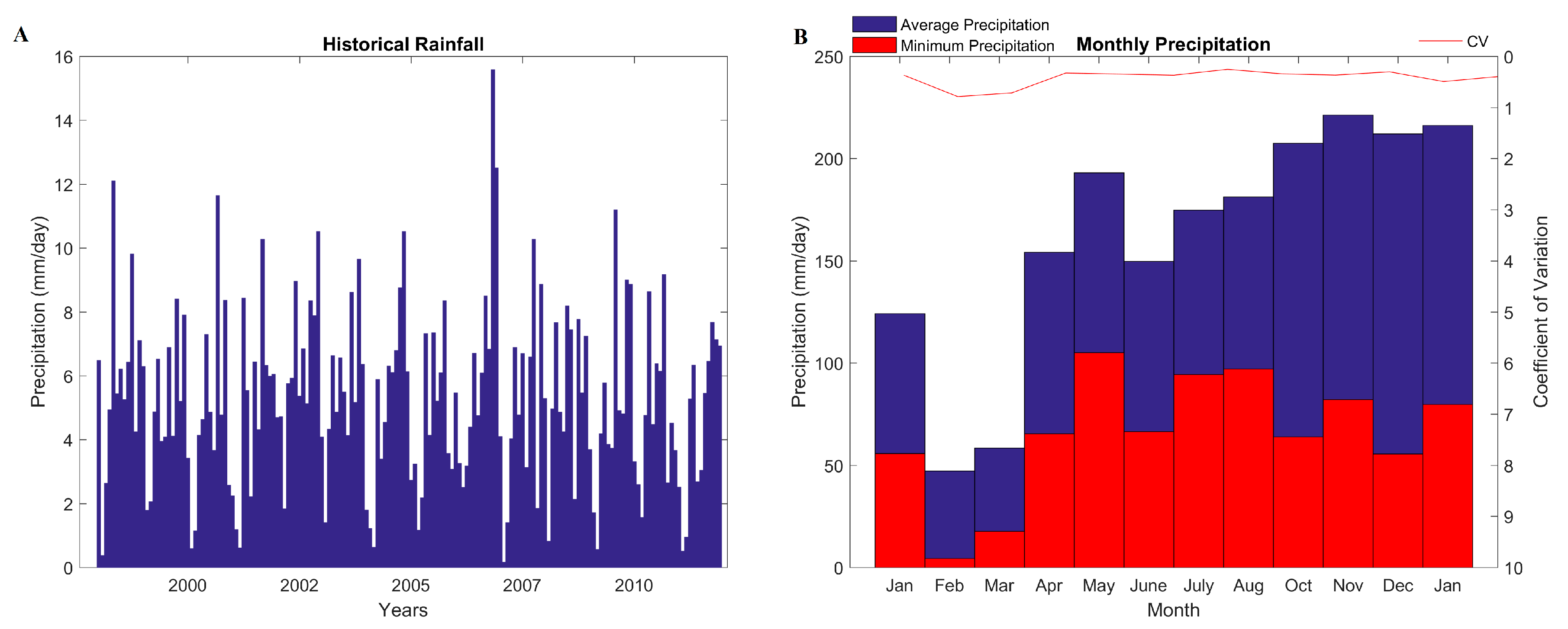
Gan Island is located in the eastern side of the Laamu atoll with latitude 1°55′ and longitude 73°32″30′ (Figure 1). As the biggest island in the Maldives in terms of land surface area, Gan Island has a land area of 598 ha with a length of 7.8 km and a width of 3.4 km, including three principal villages: Thundi, Mathimaradhoo, and Mukurimagu (Figure 1). Gan’s population has grown rapidly from 2537 persons [34] in 2005 to 4208 persons in 2009. As there are no in-situ observed daily rainfall data available, daily rainfall data from 1998 to 2011 (Figure 2A) are provided by the Tropical Rainfall Measuring Mission (TRMM). The average annual rainfall is 1930 mm/year with a pronounced wet season (October–December) and dry season (January–March). The minimum and average monthly rainfall depths are shown in Figure 2B. Typically, February and March constitute a very dry period, but also has the largest variation and CV value.
In December of 2009, the Government of Maldives conducted a groundwater investigation survey on Gan Island as part of the Maldives Tsunami Infrastructure Project. They used the electromagnetic induction (EM) method at 25 locations (green dots in Figure 1D) to provide contours of freshwater lens thickness and an estimate of total fresh groundwater volume. The total volume of fresh groundwater at the time of the study was estimated to be 14.2 million m3 (assuming a porosity of 0.3) with an average freshwater lens thickness of 8.4 m at the 25 measurement locations [35].
2.2. Model Development
2.2.1. SUTRA Modeling Code
The SUTRA (Saturated-Unsaturated Transport) modeling code [26] is used in this study to simulate groundwater flow and salt transport in the aquifer of Gan Island. SUTRA simulates groundwater flow dependent on both groundwater head gradients and fluid density differences, thus allowing the simulation of freshwater/seawater interaction and resulting in the development of a freshwater lens floating atop seawater within the aquifer sediments. SUTRA uses the finite element method to solve the coupled density-dependent groundwater flow and solute transport governing equations. Therefore, the model domain is discretized into elements and nodes. Model inputs include aquifer properties (permeability, specific yield, and specific storage), boundary conditions (e.g., specified fluid pressure and accompanying solute concentration), and forcing terms (e.g., recharge and accompanying solute concentration) applied to mesh nodes. Model outputs include fluid pressure and solute concentration at each mesh node.
2.2.2. Construction of the Gan Island SUTRA Model
In this study, a 3D SUTRA model is created to represent the aquifer of Gan Island. Compared to a 2D vertical cross-section model, which has often been used to simulate freshwater lens dynamics of atoll islands, a 3D model has the advantage of being able to specify natural boundary conditions, represent the actual shape of the coast or island surface area, simulate the effect of groundwater pumping in all aquifer dimensions, and provide an estimate of lens volumes. For the Gan Island model, salt (total dissolved solids) is designated as the solute, with 0.00089 kgsalt/kgwater (equivalent to a chloride concentration 550 mg/L) designated as the upper limit of potable water. The chloride concentration is slightly lower than the World Health Organization [36] recommended benchmark concentration of 600 mg/L, to provide conservative results. This value is therefore used to determine the spatial extent of the freshwater lens and its boundaries with the transition zone.
Due to the large domain of the island and the large number of required mesh elements and nodes, the SUTRA code was recompiled into a 64-bit executable to extend the capacity of memory allocation. In addition, subroutines within the code were implemented to allow for time-dependent fluid source/sinks terms (i.e., recharge and pumping).
ModelMuse [37]—a graphical user interface for constructing numerical models for USGS-based codes such as MODFLOW and SUTRA was used to construct the 3D finite element mesh and to generate the necessary input files containing node-by-node aquifer properties, boundary conditions, initial conditions, and fluid source/sink terms such as recharge and pumping (i.e., extraction). The procedure of constructing the model is summarized in the following steps:
Draw the domain of the island: This is accomplished by importing the island GIS shape file, generated within ArcMap, and then drawing the outline of the island. The effect of the ocean is simulated in the model, with the model domain extending out to the ocean on all sides of the island by 800 m. The ocean domain within the model was chosen to minimize the influence of the boundary conditions of fluid pressure and salt concentration on groundwater flow and salt transport within the island aquifer. The size of the ocean domain was set to double the size of the island, with the shape similar to the island.
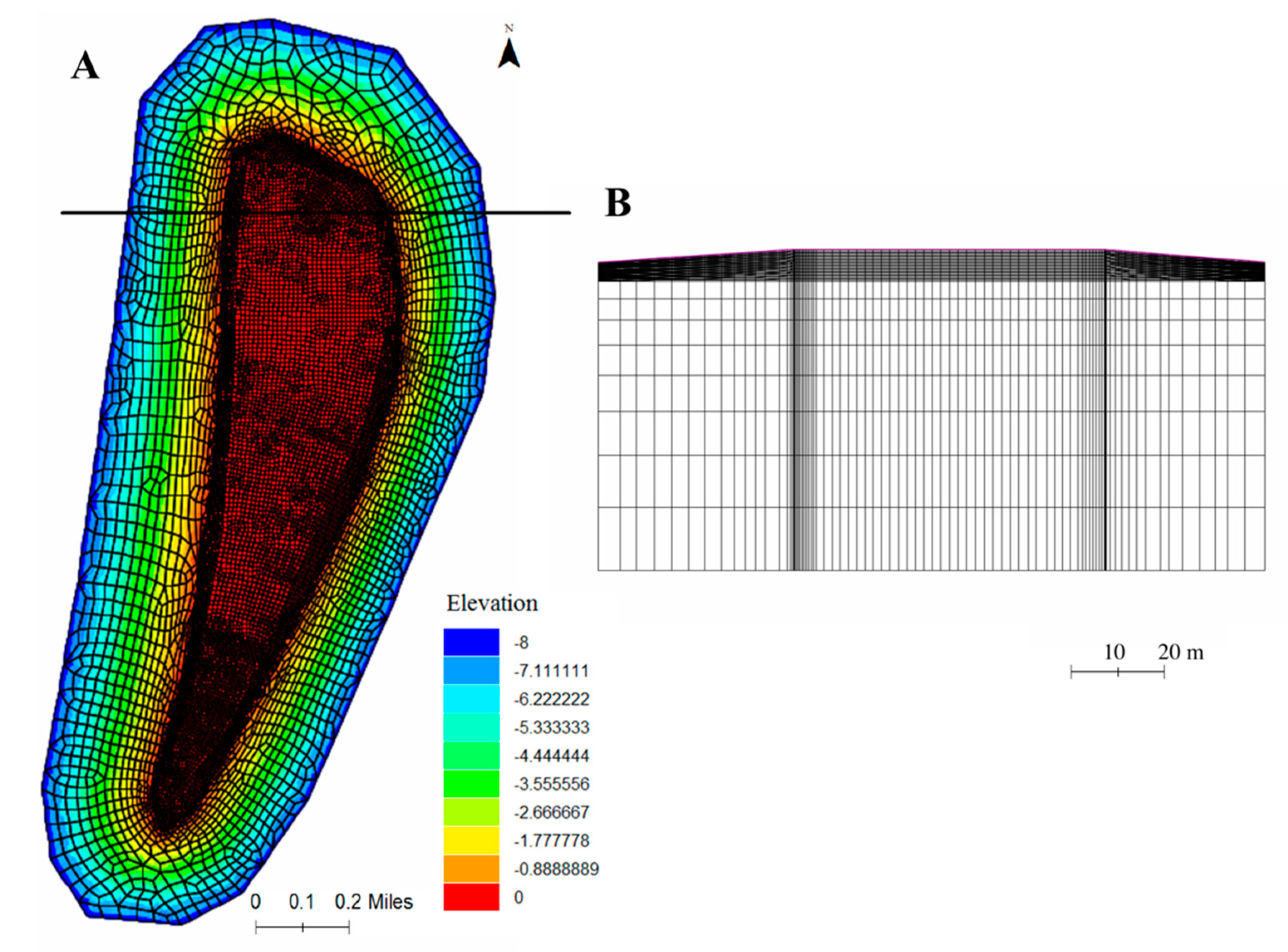
Generate the finite element mesh: SUTRA uses irregular quadrilateral elements, which are refined locally along the top of the model and along the coastal boundary where large changes in groundwater hydraulic head and salt concentration are expected during the model simulations. The elevation of island surface in the model is set to 0 m.a.s.l., since only the saturated zone of the aquifer is included in the model. However, water table storage is accounted for by assigning the top nodes a specific storage value that is equal to the aquifer specific yield, divided by half of the thickness of the finite element containing the node. The slope on the coast is set to 1%, a common beach slope for the Maldives. The surface mesh and vertical discretization of the mesh are shown in Figure 3. The layer thickness (i.e., vertical distance between nodes) near the surface is <1 m, while layers toward the bottom of the mesh have a thickness between 20 and 30 m.
Aquifer properties: The layers of the mesh are assigned to either the sandy Holocene aquifer (0–20 m below sea level) or the limestone Pleistocene aquifer (20–200 m below sea level). The Holocene aquifer was assigned a horizontal hydraulic conductivity (HK) of 15 m/day and a porosity of 0.2, whereas the Pleistocene aquifer was assigned an HK of 5000 m/day, a VK of 1000 m/day, and a porosity of 0.3, similar to other atoll island modeling studies [38].
Boundary conditions and initial conditions: The mesh nodes within the ocean domain were assigned a specified pressure that represents the pressure from overlying seawater. The nodes along the top layer of the mesh are served as locations of rainfall-derived recharge to the freshwater lens and are assigned as sources of fluid flux. The input flux to each node is calculated as the product of the recharge rate (Length/Time) and the spatial area (L2) assigned to each node. Nodes within the aquifer can also represent pumping wells, assigned as extraction points of groundwater.
The final mesh contains 30 layers for the upper (Holocene) aquifer and 8 layers for the lower (Pleistocene) aquifer, with a total of 480,000 nodes. Daily time steps are used for all simulations presented in this section.
2.2.3. Simulating Groundwater Pumping
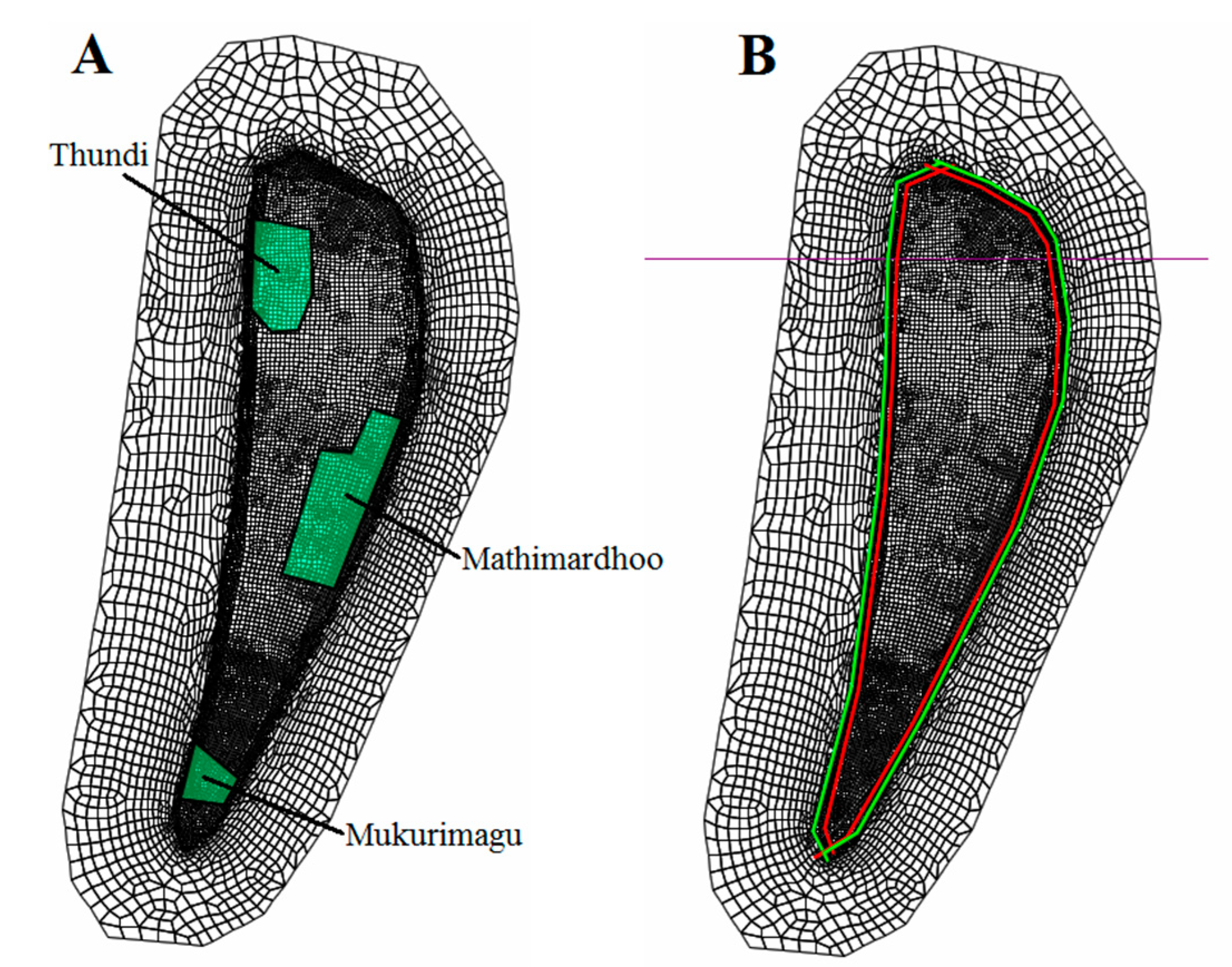
Groundwater pumping on Gan Island occurs in the three villages. One village is in the northwest of the island, one is in the mid-east, and the other is located in the south, as shown in Figure 1D. The estimate of total number of occupied houses as of October 2009 is 691, and each house has 1–2 small pumping wells or hand-dug wells [35], resulting in 700–1300 wells. Without knowing the exact location of pumps, this study defines pumping areas for the three villages, shown in the green shaded parts of the model mesh in Figure 4A. The nodes in these shaded areas are all considered as pumping nodes, with uniform pumping rates. Based on the report of Bangladesh, estimated groundwater usage is 120 L/day/person. The total water pumped from the aquifer for each of the three villages is approximated as the product of the pumping rate and the population. The pumping rate assigned to each mesh node in the village is the total water usage for the village divided by the number of nodes in the pumping area.
2.2.4. Baseline Model
The model was run historically for the 1998–2012 time period, using daily rainfall rates and estimated pumping for the three villages that increase with population growth. The potential ET was calculated using the Penman method. Daily recharge was estimated using the soil water balance model of [39], used for coral islands in the Indian Ocean. The model uses daily rainfall depths, canopy interception storage, thickness of the soil moisture zone, and the field capacity and wilting point of the soil to estimate daily soil water storage and daily percolation from the base of the soil profile (i.e., recharge to the water table). Initial conditions (fluid pressure and groundwater salt concentration) were obtained by running a long-term model simulation with constant recharge until a stable freshwater lens was obtained, i.e., groundwater salt concentration for all nodes no longer changed in time.
2.3. Model Calibration
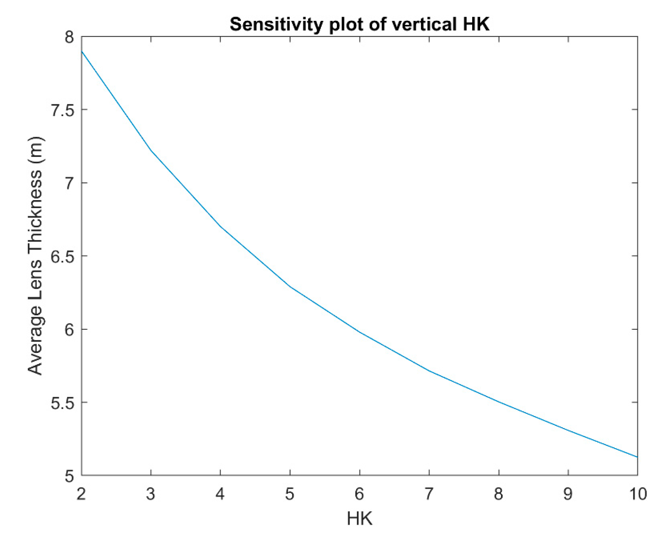
Data available for model testing include freshwater lens thickness at the 25 EM measurement sites, and the total estimated volume of fresh groundwater. As high uncertainty is associated with the capacity of EM methods to provide a lens thickness value, more confidence is given to the estimated groundwater volume. Several model parameters can be modified to provide a best match between observed and simulated spatially varying lens thickness and total groundwater volume. These include aquifer permeability and specific yield for both the upper and lower aquifer units. After many simulations to assess the sensitivity of model result trials and errors, vertical permeability of the Holocene aquifer was found to be the key factor in governing freshwater lens thickness. This parameter was therefore varied between 1 and 10 m/day to achieve the best fit between the observed and simulated freshwater lens thickness at the 25 EM measurement locations. The average lens thickness of different vertical hydraulic conductivity is plotted in Figure A1. Results are shown in Figure 5. In general, the model does not match well the point estimates of freshwater lens thickness. This is due to several island cross sections that have unexpected patterns of lens thickness, i.e., patterns that do not adhere to the theoretical freshwater lens delineation (lens-shape of the lens). The study of Bailey et al. [20] also yielded a poor match for Gan Island. More importantly, the simulated volume of the freshwater lens of 14.3 million m3 is very close to the field-measured estimate [35] of 14.2 million m3. Regardless, the value of 3 m/day shows the best match (R2 = 0.395), with an average simulated lens thickness of 9.1 m. This value was therefore chosen for all simulations in this study.
2.4. Estimating Future Groundwater Supply
Simulation results at the end of the 1998–2011 baseline model are used as initial conditions for a suite of simulations covering the 2012–2050 time period. These simulations provide an estimate of freshwater lens thickness and volume under the effects of future rainfall patterns, groundwater pumping, and sea level rise.
2.4.1. Simulating the Effect of Future Rainfall Patterns
General circulation models (GCMs) from the Coupled Model Intercomparison Project 5 (CMIP5) are used to estimate rainfall and associated recharge rates for the 2012–2050 time period, using a two-step process. In the first step, GCM output is compared to historical data of the Maldives region to select a sub-set of available GCMs that are accurate for this region. In the second step, GCM rainfall depths are downscaled to daily values.
In this first step, only a subset of the available CMIP5 GCMs are used, based on the requirement that they meet a statistical standard when compared to historical rainfall data and statistical patterns, using the process described in Fu et al. [40]. The overall performance of GCMs is evaluated using the following 7 statistical measures: mean relative error (MRE), standard deviation relative error (SDR), normalized root mean square error (NRMSE), correlation coefficient (Corr), Brier score (BS), skill score (S score), and Kendall slope (Kendall Slope). The formulas for these measures are shown in Table A1 in the Appendix A. These criteria are selected to assess accuracy in both magnitude and variance of monthly rainfall depths. For each criterion, each GCM is ranked according to its resulting value. The overall rank of each GCM is then computed using a weighted value of the individual criteria rankings, with a low value indicating a high ranking [40]:
The BS and S Score values are given weights of 0.5 since they are complementary (i.e., they are both used to evaluate the probability density function of monthly rainfall depths). Results and overall ranking for each considered GCM are shown in Table A2 in the Appendix A. As with [29], the top five GCMs are selected for Gan Island for the lowest emission scenario (Representation Concentration Pathway (RCP) 2.6, corresponding to a limited radiative forcing of 2.6 W/m2 by the year 2100), and the top 7 GCMs are selected for scenario RCP8.5 (Table A2). These 7 models are CESM1-CAM5, MIROC5, IPSL-CM5A-LR, CCSM4, GFDL-ESM2G, GISS-E2-R p1, and NorESM1-ME.
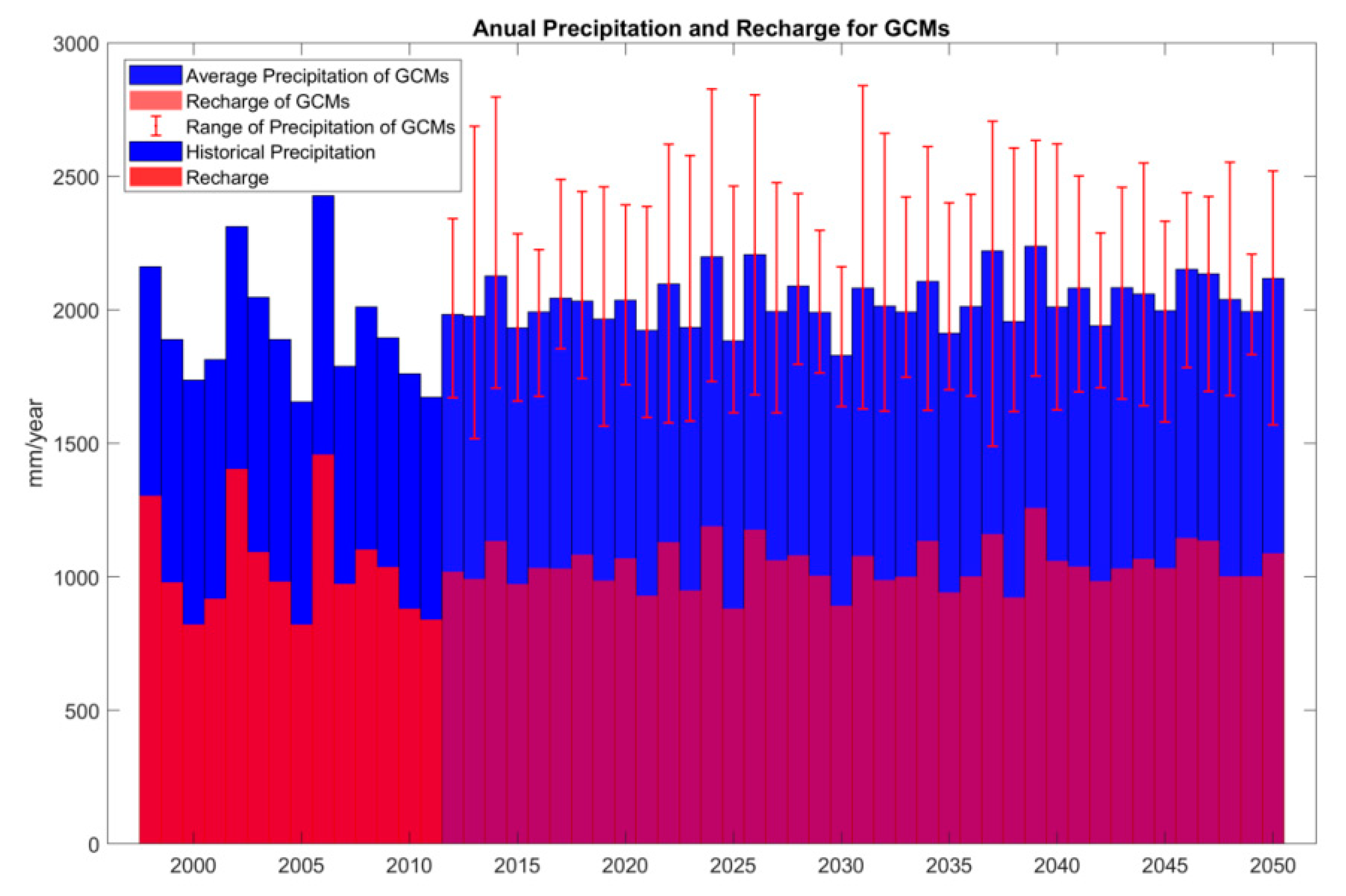
In the second step, the monthly rainfall depths from the selected GCMs are downscaled to daily rainfall data depths (mm) based on patterns in the historical daily rainfall data (1998–2011). Daily wet/dry sequences were generated using a Markov chain for historical data and fit into Gamma distribution for classification (wet/dry) and estimate daily rainfall for future wet days from GCMs [29]. Daily recharge depths (mm) are calculated from the downscaled data using the soil water balance model of [39]. The soil water balance model also includes the effect of GCM-estimated temperature on ET rates. The average daily rainfall depth during the simulation period is 5.58 mm/day, and the calculated recharge is 2.84 mm/day. More details regarding the downscaling methodology are provided in [29]. Time series of predicted rainfall data for 2012–2050 and their recharge rates are plotted in Figure 6. Error bars are included to indicate the spread of values from the GCMs.
2.4.2. Simulating the Effect of Future Groundwater Pumping
The population of Maldives has tripled in the last 35 years with an average annual growth rate of 1.76% (World average: 1.17%) [41]. With such a high growth rate, groundwater pumping can have a strong influence on groundwater resources in the Maldives, potentially leading to thinning of the freshwater lens [41,42]. Therefore, an assessment of future groundwater supply for the inhabited islands in the Republic of Maldives should include this groundwater stress. Groundwater pumping can have an especially strong effect on the freshwater lens of Gan Island, which had an annual growth rate of 13.5% between 2005 and 2010. In this study, two scenarios of pumping are included in the future scenario simulations. The “conservative” scenario assumes an annual population growth rate of 1.76%, and the “aggressive” scenario uses a rate of 9%, resulting in 2050 populations of 8456 and 132,171, respectively. For each village area (see Figure 4A), the pumping (i.e., extraction) rate for each node is estimated by multiplying the estimated annual population by the per capita water demand, and then dividing that number by the number of nodes in the village area.
2.4.3. Simulating the Effect of Future Sea Level Rise
This study estimates the relative impact of sea level rise on the thickness and volume of the Gan Island freshwater lens. The model simulates the impact of sea level rise by constructing a new model with a smaller island surface area to represent the shoreline recession that occurs due to the rise in sea level by the year 2050. The smaller model area is shown in Figure 4B. The extent of shoreline recession depends on the vertical rise of sea level and the slope of the beach. This study uses the sea level rise rate proposed by a study by Woodworth [43], which predicted a 0.5 m rise for the Maldives by the end of the 21st century and a beach slope of 1%. As a result, approximately 50 m of coastline is predicted to be lost due to sea level rise by the year 2050 (see Figure 4B). Overall, the land area of Gan decreases from 6.57 to 5.75 km2 by the year 2050.
Simulating the transient effect of sea level rise on the freshwater lens requires a continual updating of the specific pressure boundary conditions on the ocean-domain nodes. This is an extremely challenging prospect with the current SUTRA code, so the simulations assessing sea level rise impact set the boundary conditions to the 2050 conditions and then run for the 2012–2050 period. Therefore, results from these simulations are valid only for the year 2050. In addition, the use of the 2050 conditions precludes the inclusion of pumping in the sea level rise simulations, as pumping can affect the transient behavior of the lens during the 2012–2050 period, so 2050 results could not be compared between scenarios. Therefore, only a relative comparison is made between SLR and non-SLR scenarios at the year 2050, using steady recharge rates from selected GCMs.
2.4.4. Summary of Future Scenario Simulations
Six scenarios are used to assess future groundwater supply for Gan Island. Scenarios 1, 2, and 3 include rainfall from the set of GCMs (S1), conservative pumping (S2), and aggressive pumping (S3) to quantify the effect of each of these stresses individually. S4 combines GCM rainfall with conservative pumping, and S5 combines GCM rainfall with aggressive pumping. S6 includes the effect of SLR by 2050 using a steady recharge rate, which will be compared to a simulation using the same steady recharge rate and the non-SLR model mesh.
3. Results and Discussion
3.1. General Model Results
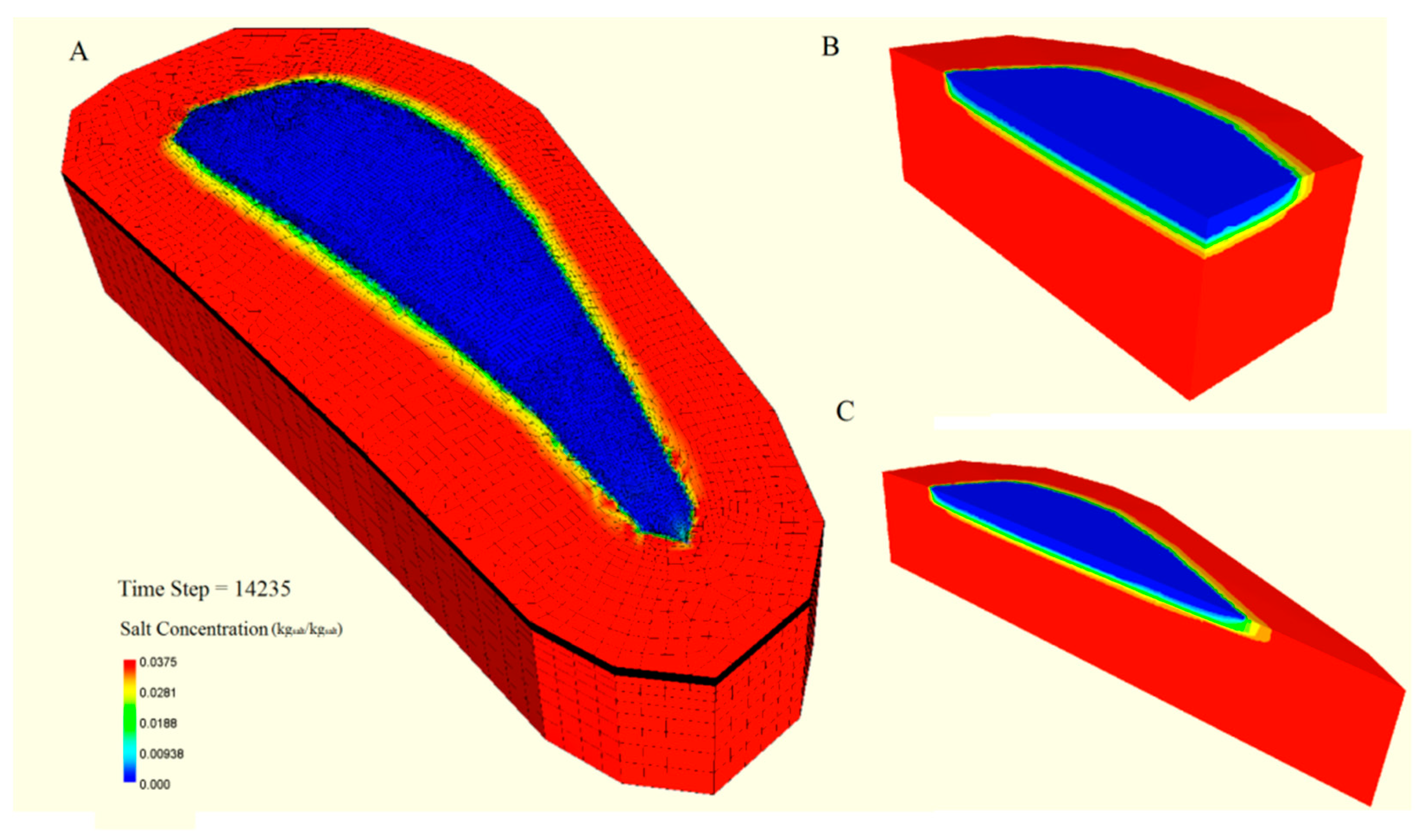
The basic simulated delineation of the freshwater lens is shown in Figure 7. Figure 7A shows the complete 3D mesh of Gan Island, with red indicating nodes with a salt concentration equal to seawater, blue indicating nodes with a salt concentration less than the potable limit, and other colors showing nodes in the transition zone between seawater and freshwater. Figure 7B,C are vertical cross sections of the island, showing the thickness and delineation of the freshwater lens. The volume of fresh groundwater is calculated by summing the lens thickness for each column of nodes, multiplying that by the area assigned to each node, and then multiplying that number by the specific yield of the aquifer.
3.2. Impact of Future Scenarios on Groundwater Supply
3.2.1. Impact of Rainfall and Population Growth
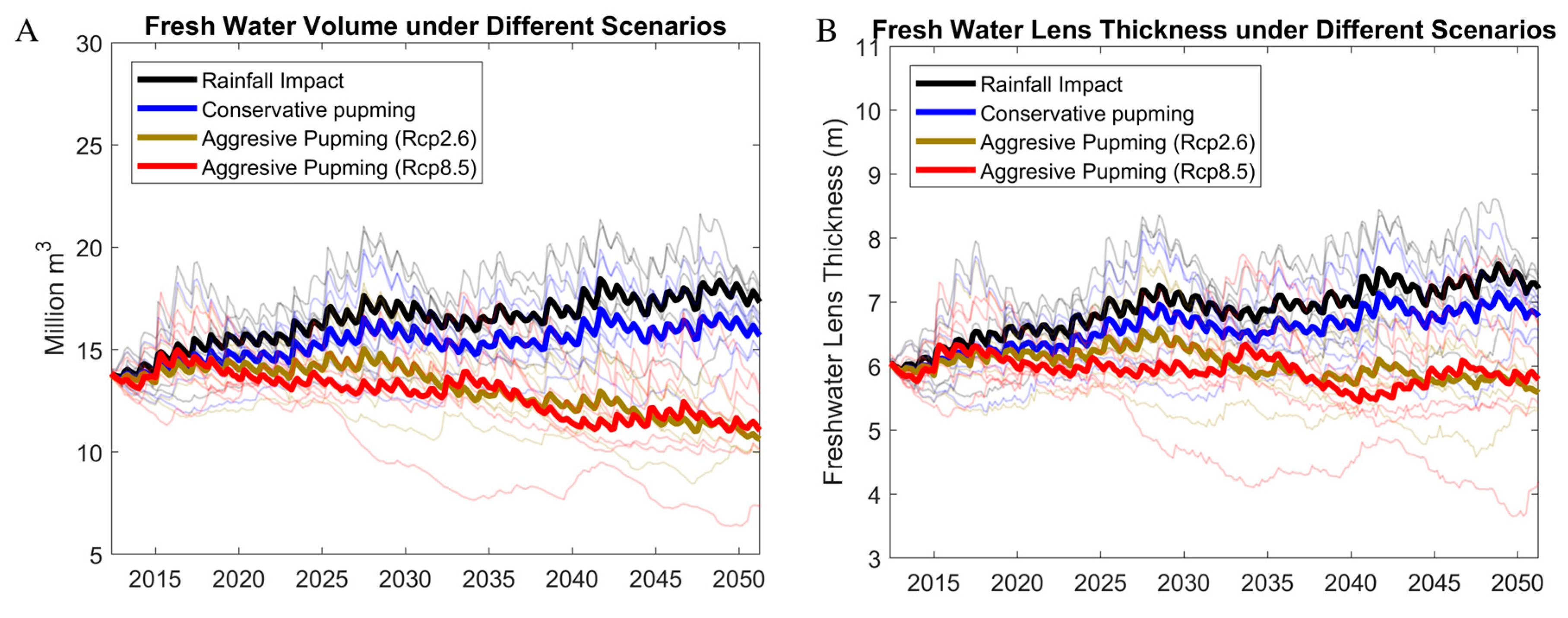
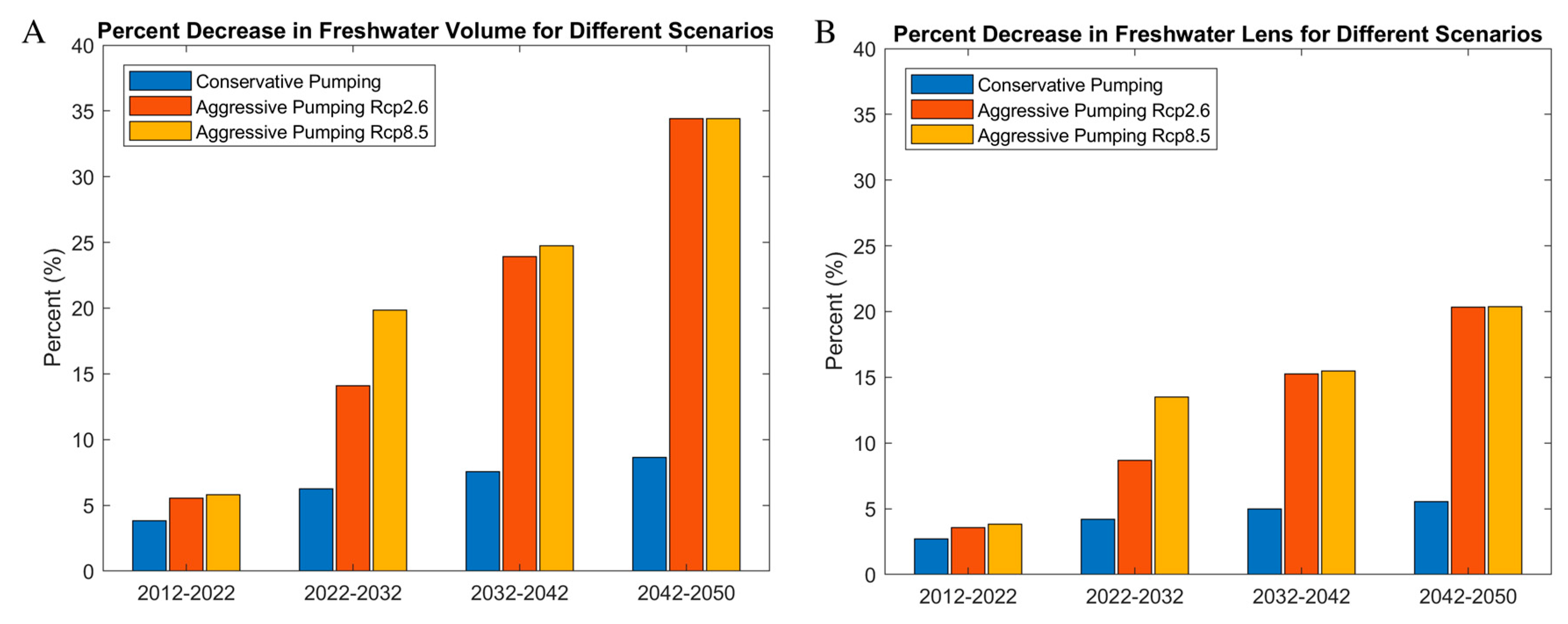
The plots shown in Figure 8 and Figure 9 summarize the results of Scenarios 1–5. Figure 8 shows the time series plot of freshwater volume (Figure 8A) and freshwater lens thickness (Figure 8B) through 2050 for Scenarios 1, 4, and 5, and Figure 9 shows the percentage decrease in freshwater volume (Figure 9A) and lens thickness (Figure 9B) for Scenarios 2 and 3 (pumping only).
For Figure 8, results are shown for the set of simulations that use GCM weather data, and the average for each scenario is shown with a bolded line. For S5 (combined rainfall and aggressive pumping), results are shown for both the RCP2.6 and RCP8.5 climate scenarios. For S1 (rainfall only; black line), the volume of fresh groundwater increased by 20% (1.4 M to 1.67 M liters) by 2050, and the lens thickness increased by around 20% (6 to 7.25 m). These results are also summarized in Table 1. Fluctuation of volume and lens thickness is due to annual wet and dry seasons. For S2 (conservative pumping only; Figure 9A), the volume and lens thickness decreased by 8 and 7%, respectively, whereas S3 (aggressive pumping only; Figure 9B) results in a decrease in volume and lens thickness by 44 and 27%, respectively. However, if rainfall changes are combined with conservative pumping (S4) (Figure 8A), then there is an increase in volume and lens thickness through 2050 by 12 and 13%, respectively. If aggressive pumping is assumed (S5), then there is a decline in groundwater supply, with volume and average lens thickness decreasing by 24 and 7%. The decrease in lens thickness is smaller than that of the volume because the lens is averaged over the freshwater area after the shrink. As expected, lens volume for Gan Island in the coming decades is predicted to be less than that reported by a recent modeling study [30], due to the inclusion of population growth and the associated increased groundwater pumping.
Therefore, a mild rate of population growth, accompanied with a comparable increase in groundwater pumping, can still result in an increase in future groundwater supply due to the increase in predicted rainfall rates from the accepted GCMS used in this study. In other words, the increase in rainfall provides a stronger effect on the freshwater lens than the increase in groundwater pumping, leading to an overall increase in the storage of fresh groundwater in the aquifer. In contrast, if population growth occurs at the same rate as 2005–2010 (>10%), then the effect of groundwater pumping will be stronger than the effect of rainfall, and there will be an overall decrease in groundwater storage through 2050.
3.2.2. Impact of Sea Level Rise
These results, of course, do not account for the effects of sea level rise. Results from S6 indicate that, in the year 2050, the lens volume and the lens thickness will be decreased by 18 and 6%, respectively, if the SLR rate used in this study occurs until 2050. Although the SLR condition at 2050 cannot be compared directly with results from Scenarios S1–S5, the simulation results indicate that SLR will result in a significant decrease in groundwater supply, likely up to 15%. Therefore, when comparing the SLR simulation with Scenario S4, in which combined future rainfall patterns and conservative pumping lead to a 12% increase in groundwater supply from 2012, the rise in sea level may offset these gains, resulting in about a 6% decrease in groundwater supply in 2050. If population growth rate is high, however, and Scenario S5 with aggressive pumping applies to Gan, the decrease in groundwater supply may be 35–40% with sea level rise rather than 24% if only rainfall and pumping are applied (see Table 1, S5 results).
These results point to the need for managing groundwater pumping on Gan Island. If moderate population growth occurs over the next several decades, and groundwater pumping rates correspond proportionally to the number of inhabitants in each village, then the groundwater supply will likely remain constant until 2050 due to the expected increase in regional rainfall rates, even if sea level rise occurs at a maximum rate. These results assume, however, that future rainfall rates coincide with output from GCMs. There are variations in GCM results, even for the best-performing GCMs in the Maldives region in relation to historical rainfall patterns, so there is inherent uncertainty in these results. However, if pumping accompanies a high population growth rate (>5%), then there will likely be a decrease in freshwater lens volume no matter the rate of sea level rise. If sea level rise occurs at maximum rates, then groundwater supply can decrease by up to approximately 40%, which could result in a strong stress on the water resources supply of Gan Island, particularly during drought periods when island residents rely solely on groundwater.
4. Summary and Conclusions
This study accessed the impacts of future climate change and population increases on the groundwater resources of Gan Island, Republic of Maldives, up to the year 2050. A 3D SUTRA groundwater flow and salt transport model was used to simulate the development and response of the island’s freshwater lens to future rainfall patterns, future groundwater pumping rates corresponding to population growth, and sea level rise, which results in shoreline recession and therefore a smaller island surface area. Modeling results yield the following conclusions for groundwater supply in the year 2050:
- If only future rainfall is accounted for, then groundwater supply on Gan Island will increase by about 20%.
- If future rainfall patterns are similar to historical patterns, then population growth rates of 2 and 9% will result in a groundwater supply decrease of 8 and 44%, respectively.
- If future rainfall patterns coincide with those predicted by global climate models, then a population growth rate of 2% will result in an increase in groundwater supply of approximately 12%, whereas a growth rate of 9% will result in a decrease in groundwater supply of approximately 24%.
- If sea level rise occurs at estimated rates of 20 cm from 2012 to 2050, then a population growth rate of 2% likely will result in a 6% loss in groundwater supply, whereas a population growth rate of 9% may result in a supply decreased by up to 42%.
Immediate results from this modeling study point to the need to manage groundwater pumping, even if rainfall rates continue to increase as indicated from global climate models. Results of course have inherent uncertainty due to the estimated rainfall rates, pumping rates, and sea level rise rate.
These results are directly applicable to other atoll islands with a similar size and population as Gan Island. Overall, the methods applied in this paper can be used to assess the future groundwater supply of any oceanic coral island.
Author Contributions
C.D. and R.B. conceived and designed this research; C.D. wrote the paper; R.B. provided professional guidance and edited the paper.
Funding
This work was supported by a grant from CWCB (COLORADO WATER BOARD CONSERVATION).
Acknowledgments
We thank three anonymous reviewers for helpful comment and suggestions that improved the content and presentation of this paper.
Conflicts of Interest
The authors declare no conflict of interest.
Appendix A

Table A1.
Statistical criteria for evaluating GCMs. The weighting factor assigned to each criterion also is shown.
Table A1.
Statistical criteria for evaluating GCMs. The weighting factor assigned to each criterion also is shown.
| Statistic Criterions | Formula | Weighting Factor |
|---|---|---|
| Mean Relative Error (MRE) | 1.0 | |
| Standard Deviation Relative Error (SDR) | 1.0 | |
| Normalized Root Mean Square Error (NRMSE) | 1.0 | |
| Correlation Coefficient (Corr) | Calculation in Matlab | 1.0 |
| Brier Score (BS) | 0.5 | |
| Skill Score (S score) | 0.5 | |
| Kendall Slope (Kendall Slope) | Calculated in Pro-UCL | 1.0 |
Table A2.
GCM performance results for monthly rainfall rates in Gan for RCP Scenario 2.6, ranking best to worst according to the total score.
Table A2.
GCM performance results for monthly rainfall rates in Gan for RCP Scenario 2.6, ranking best to worst according to the total score.
| GCM | Mean RE (mm) | Std RE | NRMSE | Corr | BS | S Score | Kendal Slope (mm/year) | Total Score |
|---|---|---|---|---|---|---|---|---|
| CESM1-CAM5 | 0.09 | 0.26 | 1.33 | 0.33 | 3.69 | 111 | −0.002 | 34.5 |
| MIROC5 | −0.12 | −0.22 | 0.97 | 0.47 | 4.33 | 104 | 0.0023 | 39 |
| IPSL-CM5A-LR | 0.19 | −0.21 | 1.04 | 0.43 | 3.93 | 102 | 0.0007 | 42.5 |
| CCSM4 | −0.14 | 0.02 | 1.08 | 0.46 | 3.95 | 104 | 0.0046 | 43 |
| GFDL-ESM2G | 0.01 | 0.17 | 1.34 | 0.24 | 4.07 | 109 | 0.0022 | 43.5 |
| GISS-E2-R p1 | 0.07 | 0.42 | 1.46 | 0.31 | 3.97 | 105 | −0.0033 | 53 |
| NorESM1-ME | −0.12 | 0.25 | 1.41 | 0.24 | 3.63 | 108 | 0.0034 | 57.5 |
| IPSL-CM5A-MR | 0.25 | 0.16 | 1.37 | 0.29 | 4.35 | 110 | 0.0054 | 64 |
| GISS-E2-R p2 | 0.08 | 0.41 | 1.44 | 0.33 | 4.49 | 96 | 0.004 | 64.5 |
| HadGEM2-ES | 0.25 | 0.52 | 1.39 | 0.53 | 6.03 | 88 | −0.0002 | 67.5 |
| NorESM1-M | −0.06 | 0.45 | 1.57 | 0.22 | 4.75 | 99 | 0.0028 | 74 |
| GFDL-CM3 | 0.14 | 0.57 | 1.45 | 0.45 | 4.93 | 95 | 0.0029 | 75 |
| GISS-E2-R p3 | 0.12 | 0.54 | 1.61 | 0.27 | 4.93 | 95 | −0.0011 | 75 |
| FIO-ESM | 0.03 | 0.30 | 1.49 | 0.19 | 3.83 | 101 | 0.0062 | 75.5 |
| GISS-E2-H p1 | 0.16 | 0.55 | 1.68 | 0.22 | 3.35 | 108 | 0.0018 | 79 |
| MIROC-ESM | 0.43 | −0.04 | 1.49 | 0.20 | 4.63 | 93 | −0.0025 | 79.5 |
| MIROC-ESM-CHEM | 0.43 | −0.14 | 1.46 | 0.17 | 4.79 | 85 | −0.001 | 81.5 |
| MRI-CGCM3 | 0.23 | 0.90 | 1.71 | 0.49 | 4.99 | 90 | 0.0031 | 93.5 |
| GISS-E2-H p2 | 0.27 | 0.49 | 1.65 | 0.25 | 4.57 | 96 | 0.0056 | 98 |
| GFDL-ESM2M | 0.26 | 0.86 | 1.78 | 0.42 | 4.93 | 113 | 0.0105 | 102 |
| CSIRO-Mk3-6-0 | 0.59 | 0.49 | 1.77 | 0.46 | 5.81 | 75 | 0.0051 | 103 |
| bcc-csm1-1 | −0.11 | 0.69 | 1.83 | 0.15 | 11.15 | 100 | −0.0083 | 113 |
| GISS-E2-H p3 | 0.31 | 0.68 | 1.86 | 0.21 | 4.01 | 99 | 0.0121 | 118.5 |
| HadGEM2-AO | 0.85 | 0.85 | 1.79 | 0.42 | 4.99 | 91 | 0.0109 | 119 |
Figure A1.
Sensitivity plot of vertical hydraulic conductivity (HK).

References
- Beswick, R. Water Supply and Sanitation, A Strategy and Plan for the Republic of Maldives, Parts 1 & 2; Report for Ministry of Health; Republic of Maldives: Indian Ocean, South Asia, 2000.
- Falkland, T. Report on Groundwater Investigations in Northern Development Region (ADB Regional Development Project; Republic of Maldives Ministry of Planning and National Development: Male, Republic of Maldives, 2001.
- Ministry of Planning, Human Resources and Environment, Government of Maldives. MPHRE Fifth National Development Plan 1997–2000; PostTsunami Environmental Assessment: Male, Maldives, 1998; Volume II.
- Roy, P.; Connell, J. Climatic Change and the Future of Atoll States. J. Coast. Res. 1991, 7, 1057–1075. [Google Scholar]
- Carpenter, C.; Stubbs, J.; Overmars, M. Proceedings of the Pacific Regional Consultation on Water in Small Island Countries, Sigatoka, Fiji Islands, 29 July–3 August 2002; ADB and SOPAC: Suva, Fiji, 2002. [Google Scholar]
- White, I.; Falkland, T.; Metutera, T.; Metai, E.; Overmars, M.; Perez, P.; Dray, A. Climatic and Human Influences on Groundwater in Low Atolls. Vadose Zone J. 2007, 6, 581–590. [Google Scholar] [CrossRef] [Green Version]
- White, I.; Falkland, T. Management of freshwater lenses on small Pacific islands. Hydrogeol. J. 2010, 18, 227–246. [Google Scholar] [CrossRef]
- Yamamoto, L.; Esteban, M. Atoll Island States and International Law; Springer: Berlin, Germany, 2013. [Google Scholar]
- Bailey, R.; Jenson, J.; Olsen, A. Estimating the ground water resources of atoll islands. Water 2010, 2, 1–27. [Google Scholar] [CrossRef]
- Ayers, J.F.; Vacher, H.L. Hydrogeology of an atoll island: A conceptual model from detailed study of a Micronesian example. Groundwater 1986, 24, 185–198. [Google Scholar] [CrossRef]
- Yamano, H.; Kayanne, H.; Yamaguchi, T.; Kuwahara, Y.; Yokoki, H.; Shimazaki, H.; Chikamori, M. Atoll island vulnerability to flooding and inundation revealed by historical reconstruction: Fongafale Islet, Funafuti Atoll, Tuvalu. Glob. Planet. Chang. 2007, 57, 407–416. [Google Scholar] [CrossRef]
- Terry, J.P.; Falkland, A.C. Responses of atoll freshwater lenses to storm-surge overwash in the Northern Cook Islands. Hydrogeol. J. 2010, 18, 749–759. [Google Scholar] [CrossRef]
- Chui, T.F.M.; Terry, J.P. Modeling fresh water lens damage and recovery on atolls after storm-wave washover. Groundwater 2012, 50, 412–420. [Google Scholar] [CrossRef]
- Presley, T.K. Effects of the 1998 Drought on the Freshwater Lens in the Laura Area, Majuro Atoll, Republic of the Marshall Islands; Scientific Investigations Report; Geological Survey (U.S.): Reston, VA, USA, 2005; p. 50.
- Barkey, B.; Bailey, R. Estimating the impact of drought on groundwater resources of the Marshall Islands. Water 2017, 9, 41. [Google Scholar] [CrossRef]
- Babu, R.; Park, N.; Yoon, S.; Kula, T. Sharp Interface Approach for Regional and Well Scale Modeling of Small Island Freshwater Lens: Tongatapu Island. Water 2018, 10, 1636. [Google Scholar] [CrossRef]
- van der Velde, M.; Green, S.R.; Vanclooster, M.; Clothier, B.E. Sustainable development in small island developing states: Agricultural intensification, economic development, and freshwater resources management on the coral atoll of Tongatapu. Ecol. Econ. 2007, 61, 456–468. [Google Scholar] [CrossRef]
- Dickinson, W.R. Pacific atoll living: How long already and until when. GSA Today 2009, 19, 4–10. [Google Scholar] [CrossRef]
- Rankey, E.C. Nature and stability of atoll island shorelines: Gilbert Island chain, Kiribati, equatorial Pacific. Sedimentology 2011, 58, 1831–1859. [Google Scholar] [CrossRef]
- Bailey, R.T.; Khalil, A.; Chatikavanij, V. Estimating transient freshwater lens dynamics for atoll islands of the Maldives. J. Hydrol. 2014, 515, 247–256. [Google Scholar] [CrossRef] [Green Version]
- Storlazzi, C.D.; Gingerich, S.B.; van Dongeren, A.; Cheriton, O.M.; Swarzenski, P.W.; Quataert, E.; Voss, C.I.; Field, D.W.; Annamalai, H.; Piniak, G.A.; et al. Most atolls will be uninhabitable by the mid-21st century because of sea-level rise exacerbating wave-driven flooding. Sci. Adv. 2018, 4, eaap9741. [Google Scholar] [CrossRef] [Green Version]
- Hay, J.E. Climate Risk Profile for the Maldives; National Disaster Management Center: Maldives, Republic of Maldives, 2006. Available online: http://ndmc.gov.mv/assets/Uploads/Climate-Risk-Profile-for-the-Maldives-Final-Report-2006.pdf. (accessed on 5 January 2019).
- Sovacool, B.K. Perceptions of climate change risks and resilient island planning in the Maldives. Mitig. Adapt. Strateg. Glob. Chang. 2012, 17, 731–752. [Google Scholar] [CrossRef]
- Peinhardt, K.A. Climate Change Vulnerabilities: Case Studies of the Maldives and Kenya. Honor Scholar Thesis, University of Connecticut, Sotrrs, CT, USA, 2014. [Google Scholar]
- Bailey, R.T.; Barnes, K.; Wallace, C.D. Predicting Future Groundwater Resources of Coral Atoll Islands: Predicting future groundwater resources of coral atoll islands. Hydrol. Process. 2016, 30, 2092–2105. [Google Scholar] [CrossRef]
- Voss, C.I.; Provost, A.M. SUTRA: A Model for Saturated-Unsaturated, Variable-Density Groundwater flow with Solute or Energy Transport; USGS Water-Resources Investigations Report, 02-4231; US Geological Survey: Reston, VA, USA, 2010.
- Langevin, C.D.; Thorne, D.T., Jr.; Dausman, A.M.; Sukop, M.C.; Guo, W. SEAWAT Version 4: A Computer Program for Simulation of Multi-Species Solute and Heat Transport; U.S. Geological Survey: Reston, VA, USA, 2008.
- Comte, J.-C.; Join, J.-L.; Banton, O.; Nicolini, E. Modelling the response of fresh groundwater to climate and vegetation changes in coral islands. Hydrogeol. J. 2014, 22, 1905–1920. [Google Scholar] [CrossRef] [Green Version]
- Deng, C.; Bailey, R.T. Assessing groundwater availability of the Maldives under future climate conditions. Hydrol. Process. 2017, 31, 3334–3349. [Google Scholar] [CrossRef]
- Alsumaiei, A.A.; Bailey, R.T. Quantifying threats to groundwater resources in the Republic of Maldives Part I: Future rainfall patterns and sea-level rise. Hydrol. Process. 2018, 32, 1137–1153. [Google Scholar] [CrossRef]
- Post, V.E.A.; Galvis, S.C.; Sinclair, P.J.; Werner, A.D. Evaluation of management scenarios for potable water supply using script-based numerical groundwater models of a freshwater lens. J. Hydrol. 2019, 571, 843–855. [Google Scholar] [CrossRef]
- Barnett, J.; Adger, W.N. Climate Dangers and Atoll Countries. Clim. Chang. 2003, 61, 321–337. [Google Scholar] [CrossRef]
- Ibrahim, M.S.A.; Bari, M.R.; Miles, L. Water resources management in Maldives with an emphasis on desalination. Maldives Water Sanit. Auth. Rep. Male Repub. Maldives. 2002. Available online: http://citeseerx.ist.psu.edu/viewdoc/download?doi=10.1.1.113.913&rep=rep1&type=pdf (accessed on 5 January 2019).
- AFD. Sewerage System Creation in 4 Islands, Maldives Tsunami Infrastructure Rehabilitation Project, Final Report; BRL Ingénierie for Agence Française de Développement: Male, Maldives, 2007. [Google Scholar]
- Bangladesh Consultants, Ltd. Groundwater Investigations Report for L.Gan; Ministry of Housing, Transport and Environment, Republic of Maldives: Male, Maldives, 2010.
- World Health Organization. International Standards for Drinking-Water, 2nd ed.; World Health Organization: Geneva, Switzerland, 1963. [Google Scholar]
- Winston, R.B. ModelMuse: A graphical user interface for MODFLOW-2005 and PHAST; U.S. Geological Survey: Reston, VA, USA, 2009.
- Bailey, R.T.; Jenson, J.W.; Olsen, A.E. Numerical modeling of atoll island hydrogeology. Groundwater 2009, 47, 184–196. [Google Scholar] [CrossRef] [PubMed]
- Falkland, A.C. Climate, hydrology, and water resources of the Cocos (Keeling) Islands. ARB 1994, 400, 1–52. [Google Scholar] [CrossRef]
- Fu, G.; Liu, Z.; Charles, S.P.; Xu, Z.; Yao, Z. A score-based method for assessing the performance of GCMs: A case study of southeastern Australia. J. Geophys. Res. Atmospheres 2013, 118, 4154–4167. [Google Scholar] [CrossRef]
- Ministry of Environment and Construction State of the environment Maldives 2011. Male Minist. Environ. Energy: Republic of Maldives. 2011. Available online: http://www.environment.gov.mv/v1/download/386 (accessed on 5 January 2019).
- Pernetta, J.C. Impacts of climate change and sea-level rise on small island states. Glob. Environ. Chang. 1992, 2, 19–31. [Google Scholar] [CrossRef]
- Woodworth, P.L. Have there been large recent sea level changes in the Maldive Islands? Glob. Planet. Chang. 2005, 49, 1–18. [Google Scholar] [CrossRef]
Figure 1.
Map of the Republic of Maldives (A), located in Indian Ocean (B), with the Laamu atoll (C) and Gan Island (D) shown on the inset figures. Gan Island has a surface area of about 598 ha and a population of 4280 located within three main villages: Thundi, Mathimardhoo, and Mukurimagu. The green dots in the Gan Island inset figure show the location of the monitoring wells used to measure groundwater level and groundwater salinity concentration.

Figure 2.
Historical monthly rainfall during 1998–2011 (A) and the average and minimum precipitation of each month during 1998–2011 (B).
Figure 2.
Historical monthly rainfall during 1998–2011 (A) and the average and minimum precipitation of each month during 1998–2011 (B).

Figure 3.
(A) Top view of the finite element mesh used for the SUTRA model of Gan Island, with colors indicating elevation (m) above sea level. The red elements indicate the surface area of the island, with the remaining elements depicting the shallow coastal areas of the island. (B) Cross section view of the mesh for the black line transect shown in Figure 3A, showing the vertical discretization of the elements to represent the aquifer.

Figure 4.
Finite element mesh used for the SUTRA model of Gan Island, showing (A) the collection of finite element nodes within each island village, and (B) the comparison of the island surface before (2012: green line) and after (2050: red line) sea level rise. The difference between the green and red lines indicates the island surface area that will be inundated by 2050.

Figure 5.
Observed vs. simulated lens thickness at the monitoring well locations shown in Figure 1, for four values of vertical hydraulic conductivity (Kv), with the red 1:1 line indicating a perfect match. Note that a small change in Kv results in significant changes in lens thickness.
Figure 5.
Observed vs. simulated lens thickness at the monitoring well locations shown in Figure 1, for four values of vertical hydraulic conductivity (Kv), with the red 1:1 line indicating a perfect match. Note that a small change in Kv results in significant changes in lens thickness.

Figure 6.
Bar plot showing annual historical precipitation, future estimated precipitation from general circulation models (GCMs), and estimated historical and future annual recharge. The blue bars represent annual rainfall depths (mm/year), and the red bars represent annual recharge depths (mm/year). The future rainfall values are the average of the selected GCMs, with error bars to quantify the spread of the GCMs.

Figure 7.
Three-dimensional view of the SUTRA finite element mesh for Gan Island for year 2050, showing the spatial distribution of salt concentration in the aquifer. Red represents the salinity concentration of seawater, and blue represents freshwater (i.e., salinity concentration = 0), with other colors representing the transition zone. (A) shows the horizontal extent of the freshwater lens on the island, and (B,C) show cross sections of the freshwater lens through the longitudinal and transverse lines of the island.

Figure 8.
Time series charts showing the results of the modeling scenarios summarized as (A) freshwater lens volume and (B) freshwater lens thickness. Bold lines indicate averages from the set of GCM rainfall rates applied to each scenario, and the light lines show the results from the set of GCM rainfall rates applied to each scenario. The black line shows the impact of Scenario 1 (only future rainfall patterns); the blue line shows the impact of Scenario 4 (future rainfall + conservative pumping); the red and gold lines show the impact of Scenario 5 (future rainfall + aggressive pumping) for both the RCP2.6 and RCP8.5 climate scenarios.

Figure 9.
Percentage decrease in (A) freshwater lens volume and (B) freshwater lens thickness for each decade of simulation, as compared to the 2012 values for Scenarios 2 and 3 (conservative and aggressive pumping, respectively). These scenarios do not include the influence of future rainfall patterns. Scenario 3 includes both the RCP2.6 and RCP8.5 climate scenarios.

Table 1.
Summary of the six model scenarios and statistics of the resulting simulated lens thickness (m) and lens volume (106 m3) in the year 2050. The grey cells with “x” are the scenarios that include the stresses. The rose and green shades indicate scenarios that result in an increase and decrease in groundwater supply, respectively.
| Scenarios | S1 | S2 | S3 | S4 | S5 | S6 | |
|---|---|---|---|---|---|---|---|
| Stresses | Rainfall Change | x | x | x | |||
| Conservative Pumping | x | x | |||||
| Aggressive Pumping | x | x | |||||
| Sea Level Rise | x | ||||||
| Results | Lens Volume (106 m3) | 16.7 | 13 | 7.8 | 15.6 | 10.6 | 11.4 |
| Standard Dev. | 0.73 | 0.79 | 0.53 | 0.8 | |||
| % Increase from 2012 | 20% | −8% | −44% | 12% | −24% | −18% | |
| Lens Thickness (m) | 7.2 | 5.6 | 4.4 | 6.8 | 5.6 | 5.7 | |
| Standard Dev. | 0.22 | 0.27 | 0.26 | 0.34 | |||
| % Increase from 2012 | 20% | −7% | −27% | 13% | −7% | −6% |
© 2019 by the authors. Licensee MDPI, Basel, Switzerland. This article is an open access article distributed under the terms and conditions of the Creative Commons Attribution (CC BY) license (http://creativecommons.org/licenses/by/4.0/).
Share and Cite
MDPI and ACS Style
Deng, C.; Bailey, R. A Modeling Approach for Assessing Groundwater Resources of a Large Coral Island under Future Climate and Population Conditions: Gan Island, Maldives. Water 2019, 11, 1963. https://doi.org/10.3390/w11101963
AMA Style
Deng C, Bailey R. A Modeling Approach for Assessing Groundwater Resources of a Large Coral Island under Future Climate and Population Conditions: Gan Island, Maldives. Water. 2019; 11(10):1963. https://doi.org/10.3390/w11101963
Chicago/Turabian StyleDeng, Chenda, and Ryan Bailey. 2019. "A Modeling Approach for Assessing Groundwater Resources of a Large Coral Island under Future Climate and Population Conditions: Gan Island, Maldives" Water 11, no. 10: 1963. https://doi.org/10.3390/w11101963
Note that from the first issue of 2016, this journal uses article numbers instead of page numbers. See further details here.