Development of a Non-Parametric Stationary Synthetic Rainfall Generator for Use in Hourly Water Resource Simulations

1
Department of Agricultural and Biological Engineering, University of Florida, Gainesville, FL 32603, USA
2
National Snow and Ice Data Center (NSIDC), University of Colorado, Boulder, CO 80309, USA
3
Department of Civil, Architectural and Environmental Engineering, Drexel University, Philadelphia, PA 19104, USA
4
Department of Earth and Environmental Engineering, Columbia University, New York, NY 10027, USA
*
Author to whom correspondence should be addressed.
Water 2019, 11(8), 1728; https://doi.org/10.3390/w11081728
Submission received: 6 June 2019
/
Revised: 26 July 2019
/
Accepted: 26 July 2019
/
Published: 20 August 2019
(This article belongs to the Special Issue Stochastic Modelling of Hydrometeorological Processes for Engineering Applications)
Abstract
:This paper presents a new non-parametric, synthetic rainfall generator for use in hourly water resource simulations. Historic continuous precipitation time series are discretized into sequences of dry and wet events separated by an inter-event dry period at least equal to four hours. A first-order Markov Chain model is then used to generate synthetic sequences of alternating wet and dry events. Sequential events in the synthetic series are selected based on couplings of historic wet and dry events, using nearest neighbor and moving window methods. The new generator is used to generate synthetic sequences of rainfall for New York (NY), Syracuse (NY), and Miami (FL) using over 50 years of observations. Monthly precipitation differences (e.g., seasonality) are well represented in the synthetic series generated for all three cities. The synthetic New York results are also shown to reproduce realistic event sequences proved by a deep event-based analysis.
1. Introduction
Management of runoff is one of the most important water quality goals in urbanized watersheds. Accurate estimation of runoff from urban catchments requires hourly or sub-hourly precipitation time series. While historical precipitation time series at this temporal resolution can be used to drive any of the hydrologic and hydraulic models (e.g., USEPA SWMM, SUSTAIN, WinSLAMM, etc.) commonly used for urban simulations, their runoff predictions are directly determined by the particular sequence of precipitation in the historical record that is input. Without uploading additional precipitation time series one by one, none of the existing urban hydrologic models can be used to efficiently investigate the role that alternative patterns of precipitation could have on runoff predictions.
Risk-based hydrologic investigations, for example those focusing on agricultural water use, reservoir/watershed management, and climate change impact assessments, typically use synthetic precipitation series. However, the precipitation sequences used in these kinds of studies typically have a coarser temporal resolution (e.g., daily, monthly) due to the relatively long time scales under consideration in such investigations [1,2,3].
Most synthetic precipitation generators use stochastic methods that assume rainfall is a random process that can be modeled statistically based on the observed characteristics of actual precipitation records. Stochastic precipitation generators have been developed and used extensively for flood risk management [4], sizing reliable rainwater harvesting systems [5], and other water resource management tasks [6].
Stochastic precipitation generators create long continuous Markovian sequences of precipitation through a variety of methods [7]. Poisson white noise (PWN) method was one of the earliest tools in modelling precipitation by statistically generating storm event arrival time, event duration, and precipitation amount [8,9,10] with independent distributions, usually Poisson for time and duration and Gamma for precipitation. In another method, a precipitation event was conceptualized as an assembly of a number of subcells with aggregation allowed by Neyman-Scott rectangular pulse (NSRP), which is the combination of Poisson rectangular pulse model [11] and cluster modelling on the spatial distribution of galaxies [12]. Under this methodology, Poisson or Geometric distributions are typically assumed for arrival time and the precipitation sub-cells are assumed to occur as rectangular pulses. Other similar studies include [13,14,15,16,17,18]. Although extensively studied [19,20,21], parameter estimation is always a big challenge for PWN and NSRP models “even when using physical considerations” [22] due to the strong assumptions on statistical distributions. Amendment is required for the parameters in the underlying distributions when changing location or temporal aggregation scales. Moreover, since the dynamics and behavior of the precipitation process is too complex and chaotic [23] to be fully approximated by statistical assumptions on distributions and pulses, the variety of features embedded in the real data, such as a limited record, unusual skew, outliers, and a long tail, etc., may impair the accuracy of the parameter fitting and, in turn, reduce the reliability of the water resource modeling.
To avoid the parameter calibration inherent in stochastic models and improve the portability of precipitation generators, non-parametric methods may be used. Using Kernel density estimation [24,25] and K nearest neighbors (KNN) [25], the probability density function from the historical observation could be represented in a conditional bootstrapping approach [26]. Lall and Sharma [27] pioneered this method in modelling hydrological time series data. Successive studies include [5,28,29,30,31,32,33]. Although non-parametric methods have been tested before, most existing non-parametric weather generators operate at daily time scales or above and are of limited value in simulating Hortonian runoff generated instantaneously whenever precipitation intensity exceeds the landscape’s infiltration capacity. To incorporate historical precipitation uncertainty into probabilistic simulations of Hortonian runoff, synthetic precipitation data is needed at much finer temporal scales. To that end, this paper introduces a new, hourly non-parametric synthetic precipitation generator. The generator is incorporated into the Low Impact Development Rapid Assessment (LIDRA) tool to enable robust simulation and rapid comparison of distributed “green” approaches to urban runoff reduction in different locations. The paper is structured as follows. First the moving window, KNN, stochastic process, and the Markov Chain processes used in the development of the algorithm are presented. Next, the accuracy of the precipitation generation technique is validated through comparison of the synthetic values to observed monthly distributions of average event duration and average event precipitation depth for New York City (NYC). Finally, historical precipitation from New York, NY (1948–2011); Syracuse, NY (1948–2010); and Miami, FL (1996–2010) are used to test the portability of the synthetic generator. It should be noticed that, although non-parametric methods can be used to model extreme events, that is not the purpose of this paper. The study focuses on green infrastructure’s ability to cumulatively reduce stormwater runoff over time, rather than green infrastructure’s impact during extreme flooding events.
2. Methods
To generate synthetic precipitation time series, both the event state (wet or dry) and the precipitation amounts need to be estimated. For precipitation generators involving daily time steps, a multi-state Markov Chain algorithm is typically employed [30]. For example, the probability of the next day’s state being wet or dry is conditioned by the current day’s state. Once the daily state has been determined, researchers use a variety of methods, including bootstrapping or distributed sampling, to generate precipitation amounts for each wet day derived from historic observations.
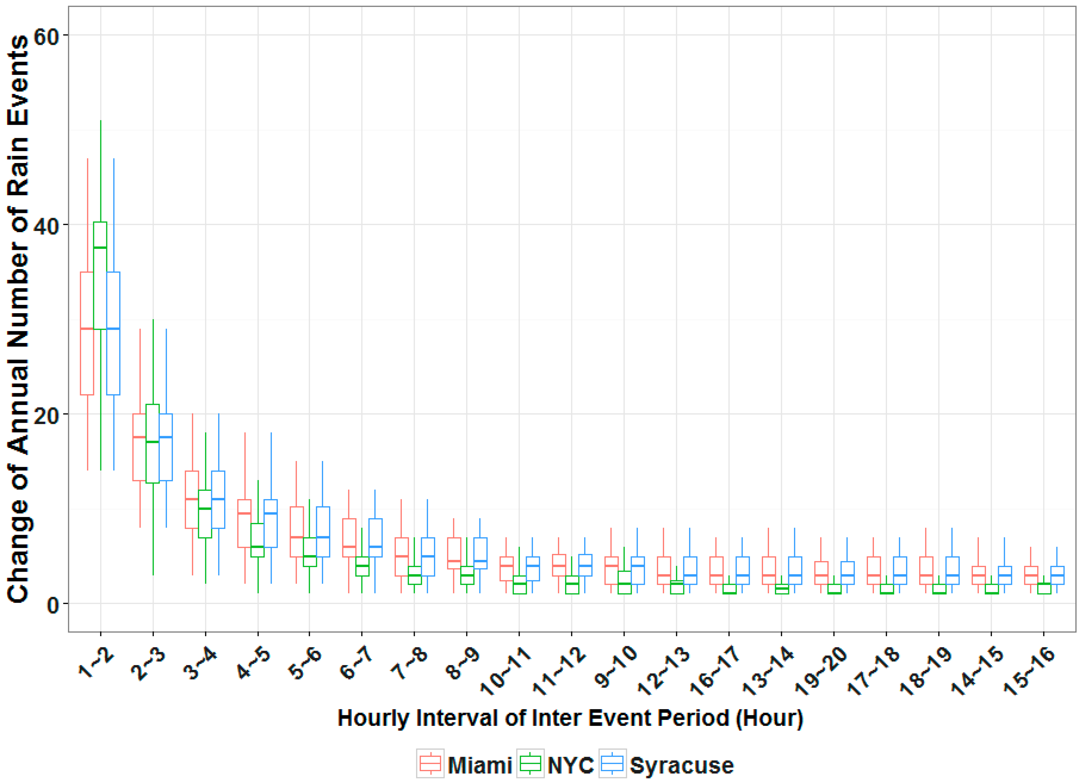
In sub-daily time scales, a similar approach can be employed by considering each rain storm as a separate event. Since individual rain storms typically span multiple hours, and may include brief periods of no rain, a technique for discretizing a continuous precipitation record into alternating wet and dry events is required. In this paper, precipitation data from NYC, Miami, and Syracuse were analyzed specifically to select an Inter Event Dry Period (IntEDP) that is suitable for synthetic precipitation generation in different climatic zones. IntEDP values of 1–20 h were applied to over 50 years of historical precipitation observation from the cities. The corresponding number of events per month based on different IntEDPs are plotted in Figure 1. While the number of events differs across different cities, shorter InEDP results in more events per month in all three locations. Precipitation in Syracuse is broken down to a mean of more than 50 events per month using a one hour IntEDP, while in NYC and Miami, this same IntEDP yields on average only 14 and 30 events, respectively. These differences are due to different atmospheric causes of precipitation in the flat coastal cities (NYC, Miami) and the higher elevation and more inland city (Syracuse).
In all three cities, the number of enumerated wet events decreases faster until the IntEDP reaches 4 h. When IntEDP > 4 h, the number of wet events obtained is much more stable. Given that the meteorological causes of precipitation in these three locales differ significantly, a four-hour IntEDP is thus considered robust, and appropriate based on the portability goal set for this particular generator.
Using the 4 h IntEDP, synthetic series are assembled non-parametrically as alternating sequences of wet and dry events sampled from the historical record, with the wet event duration and amount both determined by the characteristics of the preceding dry event. In contrast to parametric generators that define the state and amount through separate processes, both wet event duration and amount are defined simultaneously in this approach, since they are sampled directly from the historical record.
Seasonality is considered explicitly in the generator using a “moving window” approach [32]. A 30-day “window” centered at noon on the day of interest is defined. Seasonal variations are assumed not to exist within the window, regardless of the time of year. Within the moving window, k nearest neighbor (KNN) methods are embedded in the resampling process so that only the most likely events from within the moving window associated with the end of a similar previous event can be appended to the evolving synthetic sequence. The integer, k, is selected using the approach introduced by Lall and Sharma [27]:
where, n is the total number of appropriate events (wet if preceding event was dry, and dry if preceding event was wet) within a given moving window, and k is the number of nearest neighbors from which a subsequent event is randomly selected.
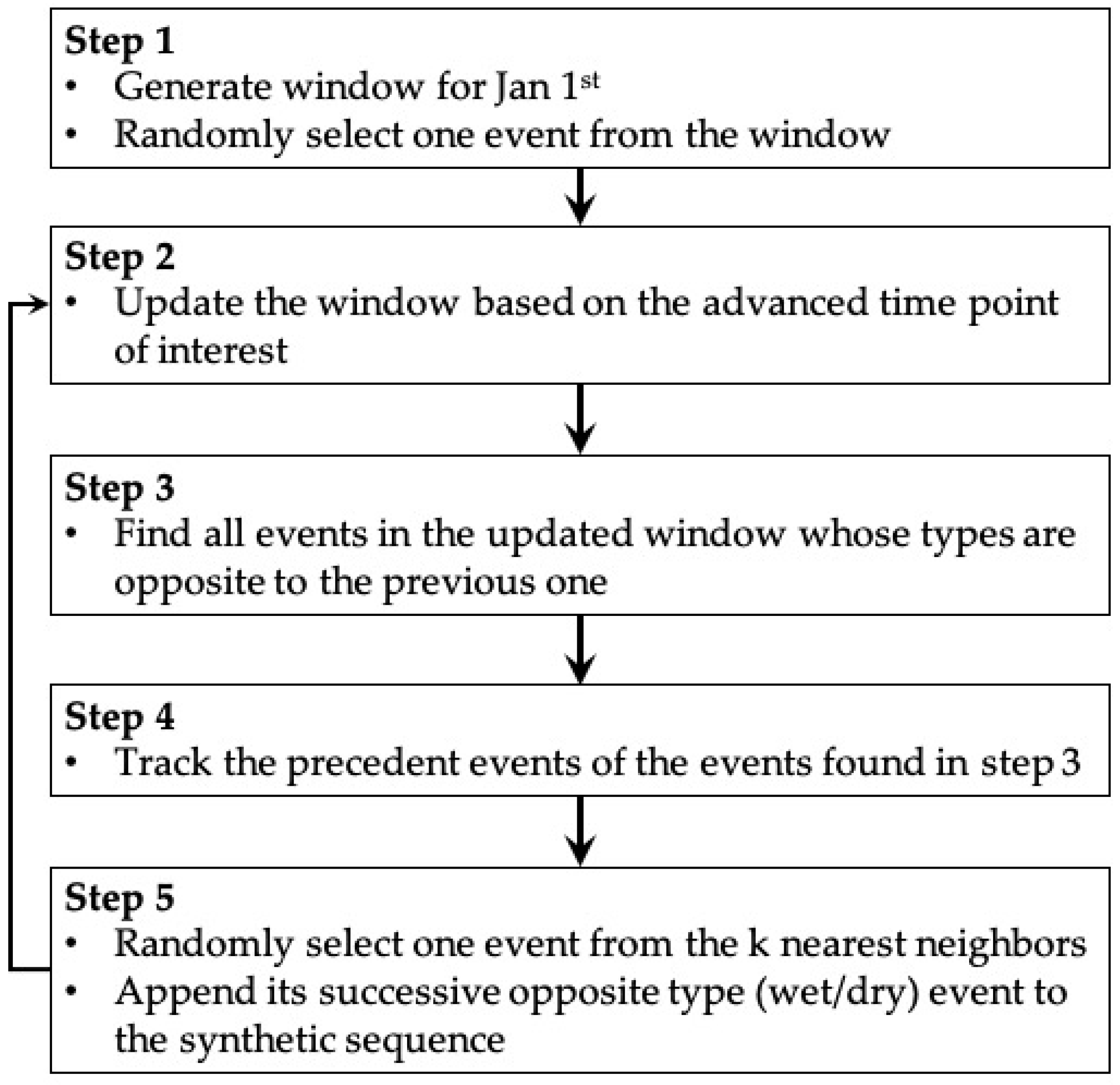
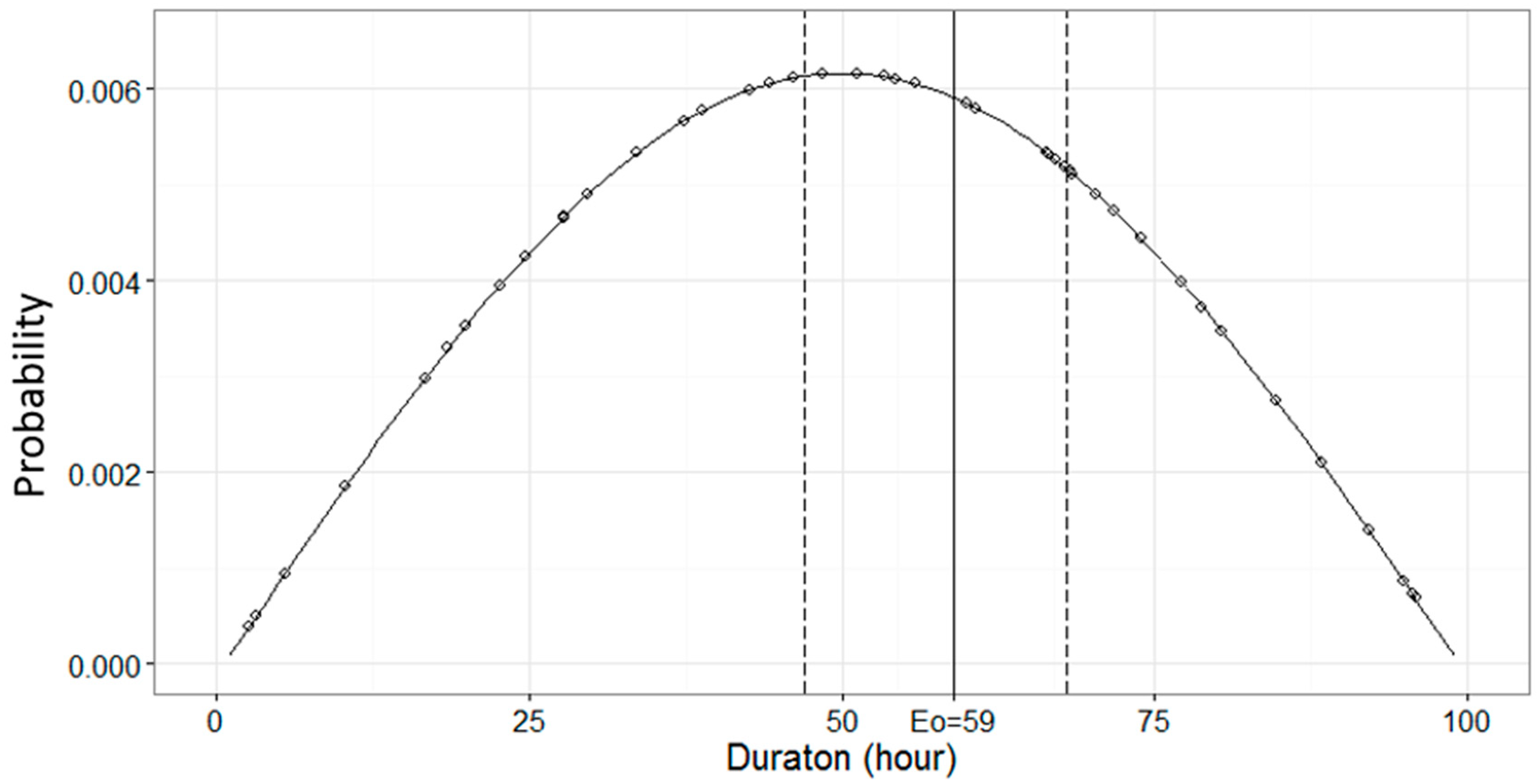
The full generation procedure is diagramed in Figure 2, as a Markov Chain process. An example is shown in Figure 3. The historical event sequence can be expressed as, for example, {d1, w2, d3, w4, …, wi, di+1, wi+2, …}, where d and w represent dry events and wet events, respectively. The procedure starts by centering a window on 12:00 on January 1st for the year of interest, where J is the indexes set of the events (dry/wet) within this window. In this example, one event wo, where o ∈ J is selected randomly as the starting point (Step 1). A new window is then created and centered on the time step advanced by wo (Step 2). Next, all dry events, the opposite type to wo, in the window determined by Step 2 (121 for this example) are extracted (Step 3); the indexes set is labeled as M. These events, Ed = {dx|x∈M}, are the pool from which the next event is selected (Step 3). The duration of wo is compared to the duration of Ew = {wx−1|x∈M} (circles in Figure 3), each preceding neighbor of events in Ed = {dx|x∈M} (Step 4). For this example, the k (11 = ) events Ewk = {wy|y∈KNN} are chosen with durations most similar to wo, shown between the dashed lines in Figure 3. One event is chosen randomly from the Edk = {dy+1|y∈KNN} as the next event in the synthetic precipitation time series. The Markov Chain processes then loops back to Step 2, with the window pushed forward by the chosen event. The process continues in this way until a complete synthetic series is generated.
Conceptually, this is a first order Markov-chain model using the event duration as the condition to sample synthetic events from historical observations. By alternating event types between wet and dry, the autocorrelations of events, such as wet vs. wet, dry vs. dry, wet vs. dry, on lag 1 is inherently preserved. For coarser scale, the moving window constrains the sampling candidates within a similar period each year, so that the seasonal periodicity can be represented as well [31]. Many researches treat precipitation amount as a statistically independent variable to event arrival time or event duration [12,13,14,19,20]. Yet, duration and amount are two physically associated dimensions for precipitation. Their underlying connection can be an integral with other characteristics [34]. This model, as a single variable Markov-chain, directly uses the precipitation information associated with each sampled event as the synthetic series.
Historical hourly precipitation records from NYC’s LaGuardia Airport, Syracuse Hancock International Airport, and Miami International Airport were used to generate 100 sets of 30 years of synthetic hourly precipitation series for all three cities. Because the synthetic series from each city were created by resampling historical observations, the synthetic series are stationary, and represent the historical variability in the data about the mean. Statistical characteristics of the synthetic series are expected to be similar to those of the respective historical records.
3. Results
The synthetic series were compared to historical observations. The model is validated using data from all three cities. As seasonality representativeness is a general challenge for synthetic precipitation generation, the validity of this method could be explored by investigating the seasonal shifting of precipitation patterns.
3.1. Event Based Analysis on NYC
Instead of lumping all events to see the overall distribution of event duration or precipitation amount, which are usually extremely skewed, the aggregations of these variables whose distributions are close to normal, based on central limited theorem, were explored. A monthly time step is employed as the basis on which the mean and standard deviation (SD) on Wet Event Duration (WED), Dry Event Duration (DED) and Wet Event Precipitation (WEP) were computed. To compare months across years, monthly distributions of these variables were computed. Such an aggregation process eliminates the bias from the number of events in different simulations when using an overall summary. For example, a particular month with many simulated short events could be weighted more heavily in calculating the overall mean than that same month in a subsequent year, if that second month contains fewer but longer events.
Since NYC presents the least seasonality among all the study cities, it was chosen to validate the seasonality of the synthetic data. Validated on the NYC data, the model was considered valid for the other two cities with more significant seasonality. The validation process compares the observed and predicted values listed below:
- Mean and SD of Wet Event Duration (WED)
- Mean and SD of Dry Event Duration (DED)
- Mean of Wet Event Precipitation (WEP) with different duration categories
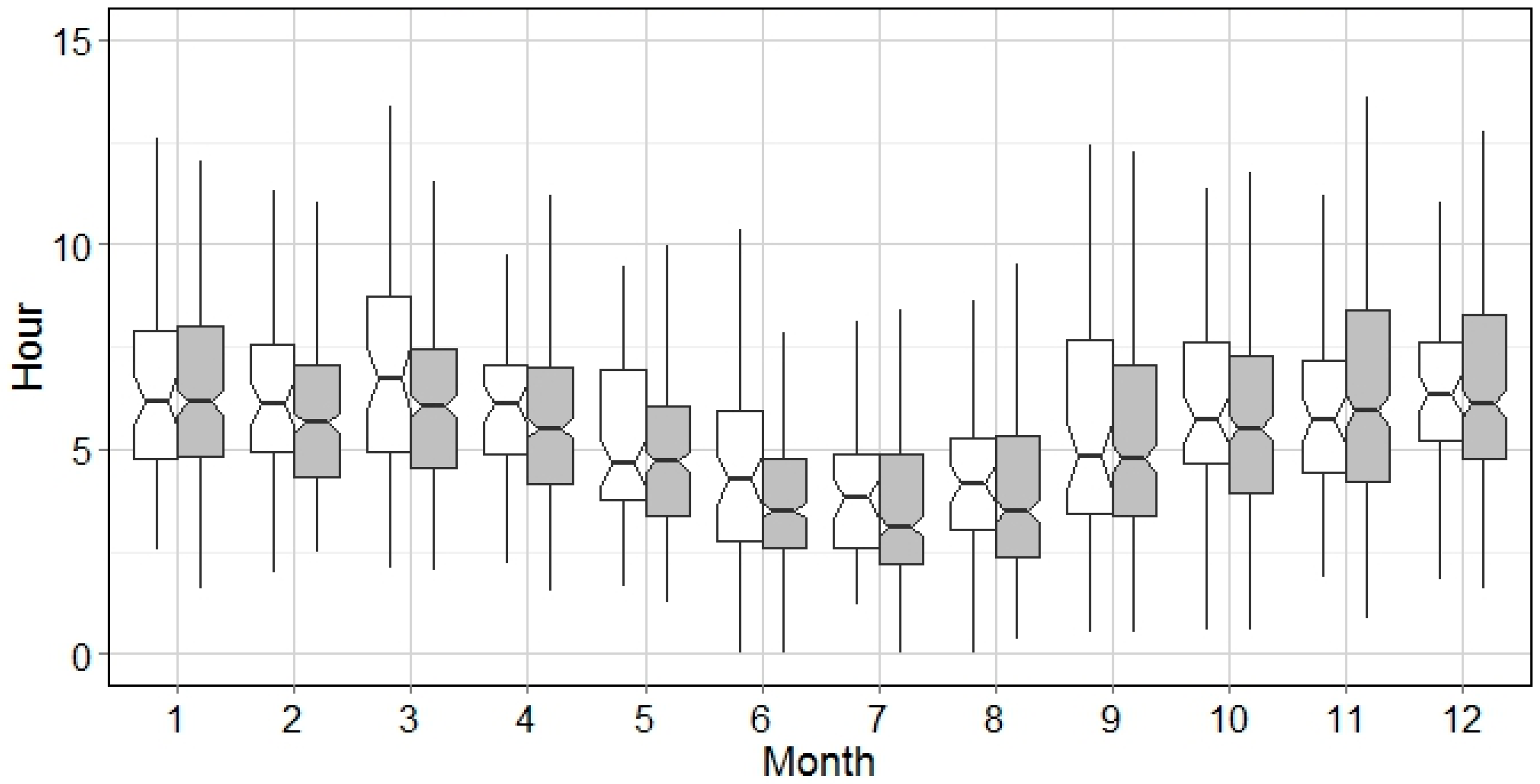
The analysis reflected by Figure 4, Figure 5, Figure 6, Figure 7, Figure 8, Figure 9, Figure 10 and Figure 11 are event-based statistics, such as mean and SD of WED, mean and SD of DED, and mean of WEP. Each event belongs to the month associated with its first hour. These measures are summarized by every month in the historical and synthetic precipitation series.
Because this algorithm is event-based, it can more robustly represent the event characteristics than the monthly precipitation. Therefore, we introduced a confidence interval notch in these plots to more clearly compare the event metrics. According to Chambers [35], if the notches of two plots do not overlap this is ‘strong evidence’ that the two medians differ.
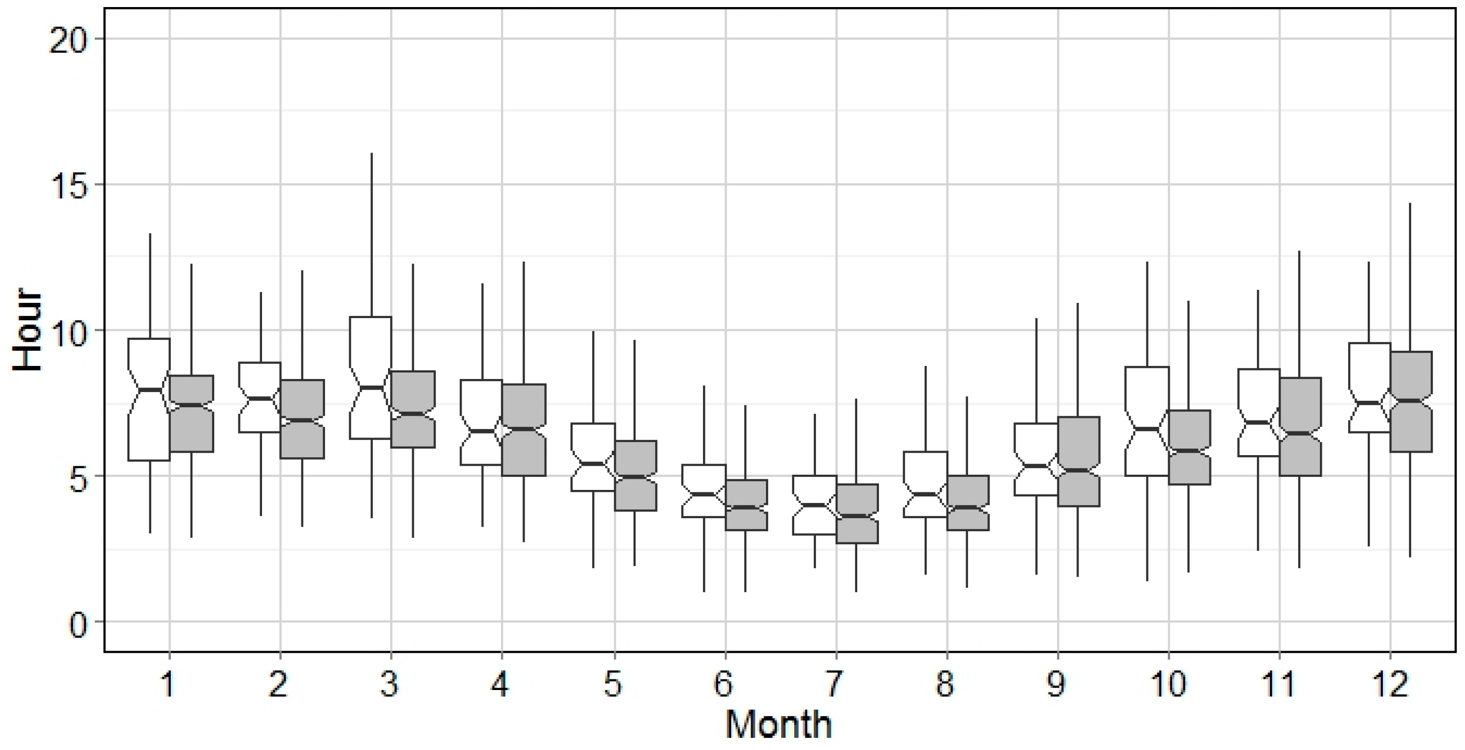
Figure 4 and Figure 5 compare the mean and SD of WED, respectively. Figure 4 clearly shows seasonality, with a long monthly average WED, about 8 h, in winter, October–March, and short monthly average WED, about 3 h, in summer, April–September. The medians for both historical and synthetic series are statistically equal (notches overlapping) for all months. Similar seasonal trends can also be found in the SD plot (Figure 5). Although the boxplots for the historical and synthetic series in April, June, and July are not obviously overlapping in the notch area, we still consider that this is a similarity with effects of seasonality smoothing.
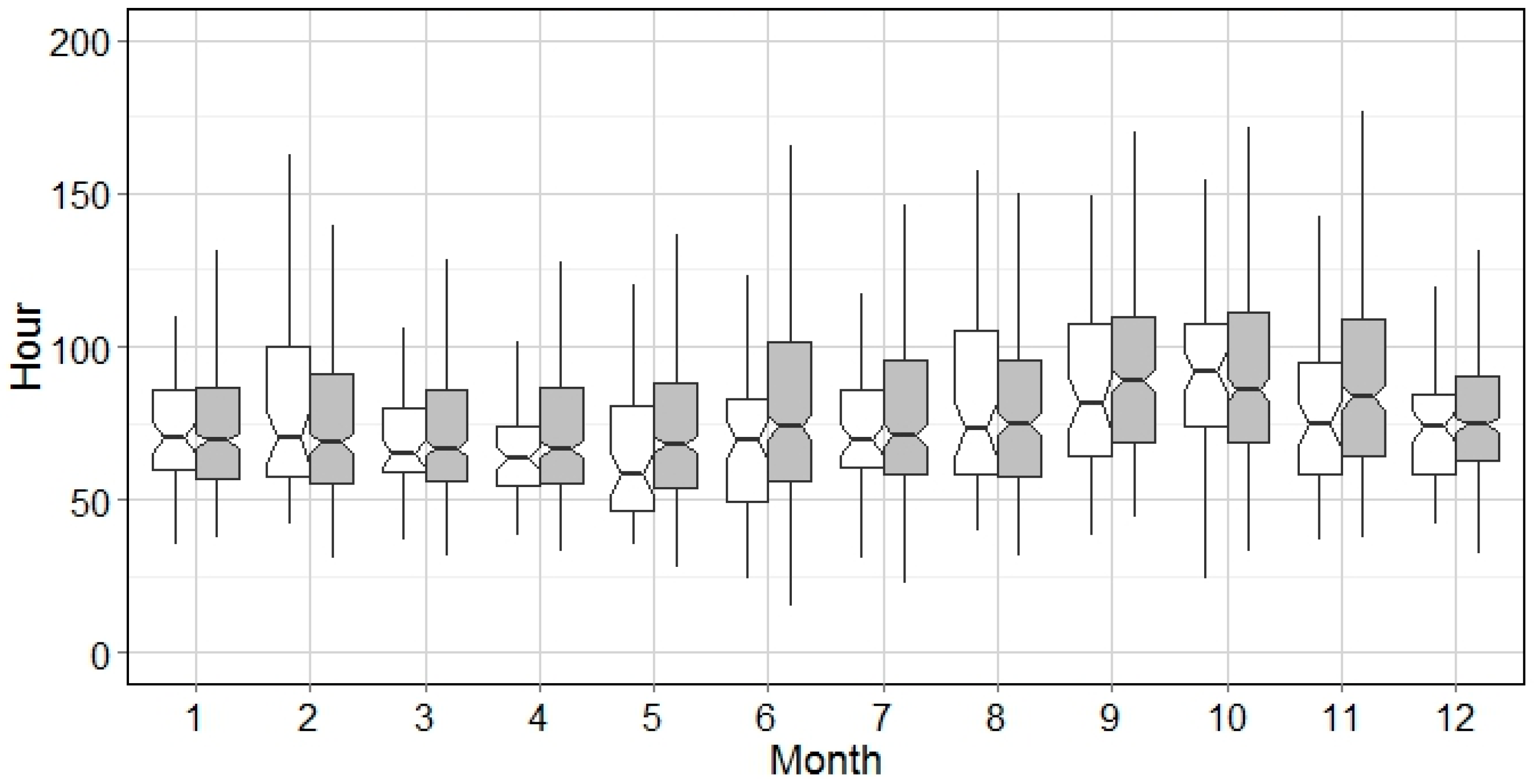
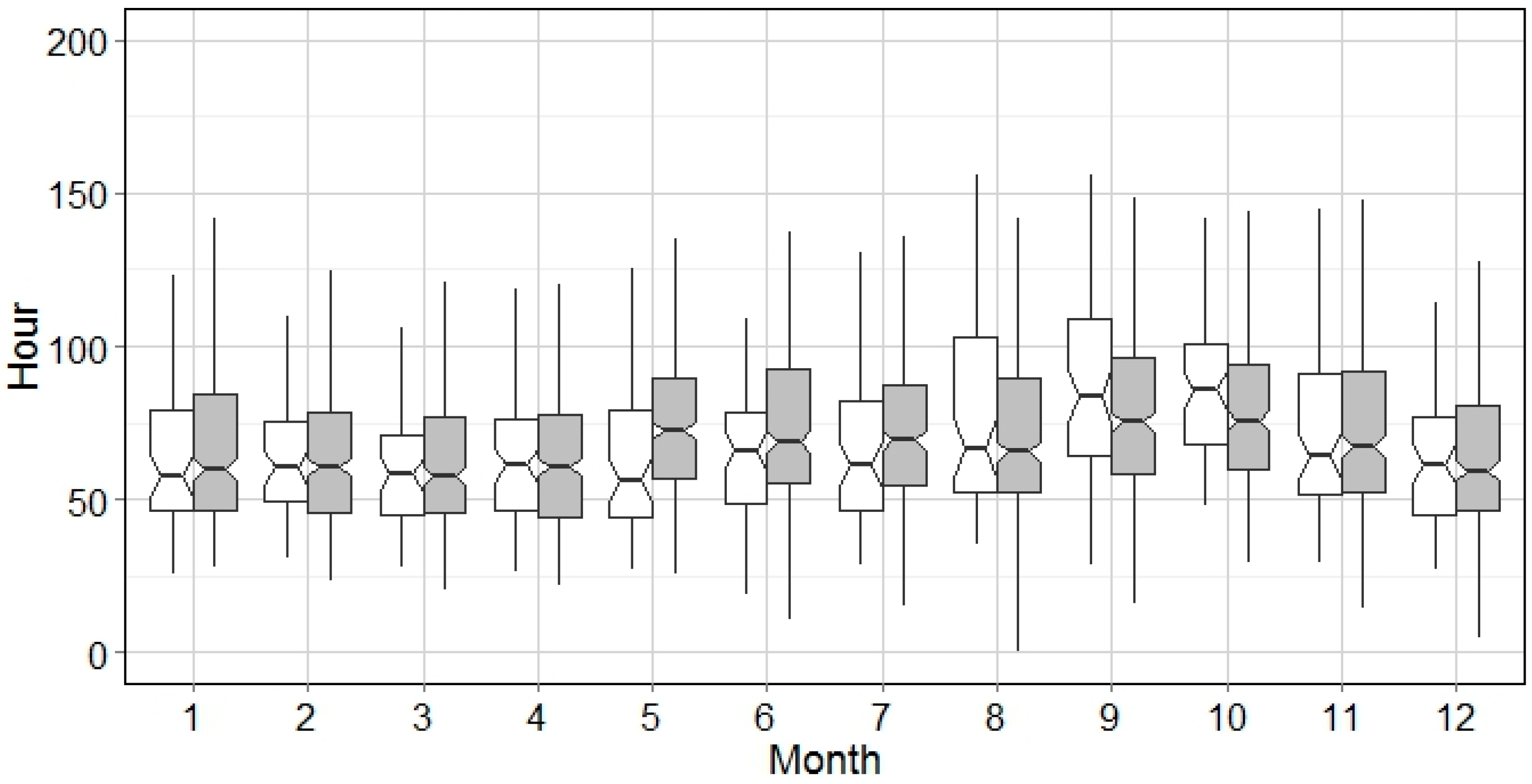
Figure 6 and Figure 7 display the mean and SD of DED, respectively. The similarity of historical series and synthetic series is well supported in these two figures as the notches overlapping can be obviously observed. Although May deviates slightly, it is acceptable given that it is a transition month between different seasons.
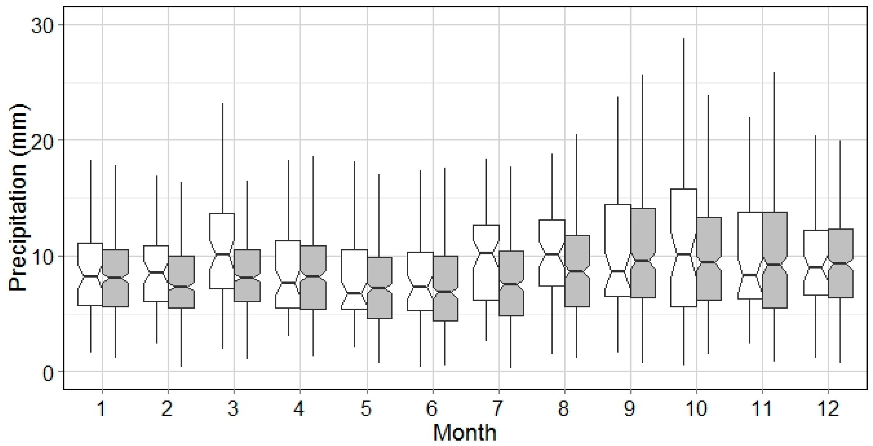
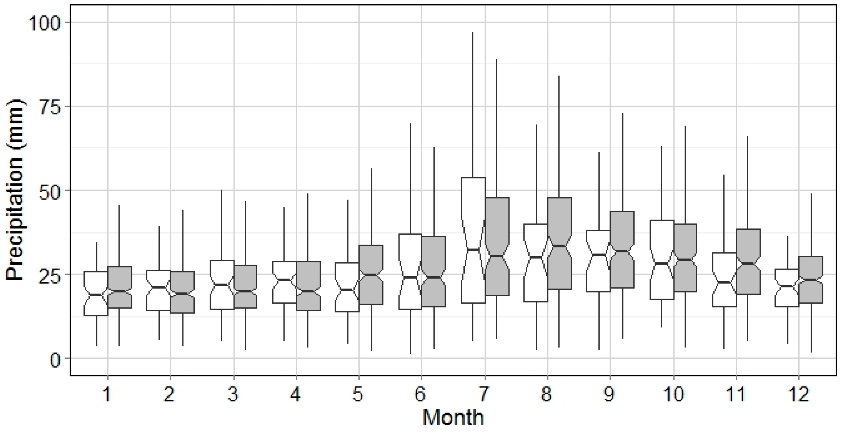
Figure 8 displays the mean of WEP for each month. Medians of monthly average WEP range from 7.5 mm in spring to 10 mm in fall. Significant difference can be found in March and July due to the sudden seasonal changes that occur then. Both the median and the variance show seasonal trends, indicating that intensive single rain events occur more frequently from July–December. This period coincides with the summer thunderstorms and the hurricane season.
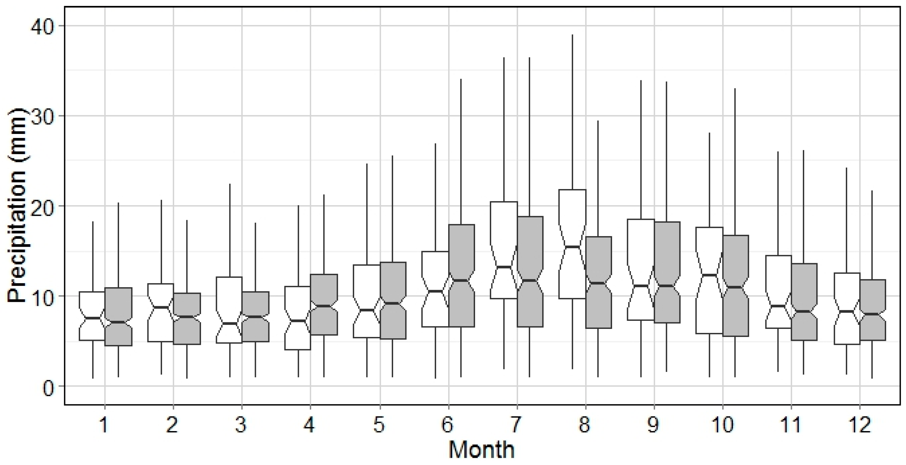
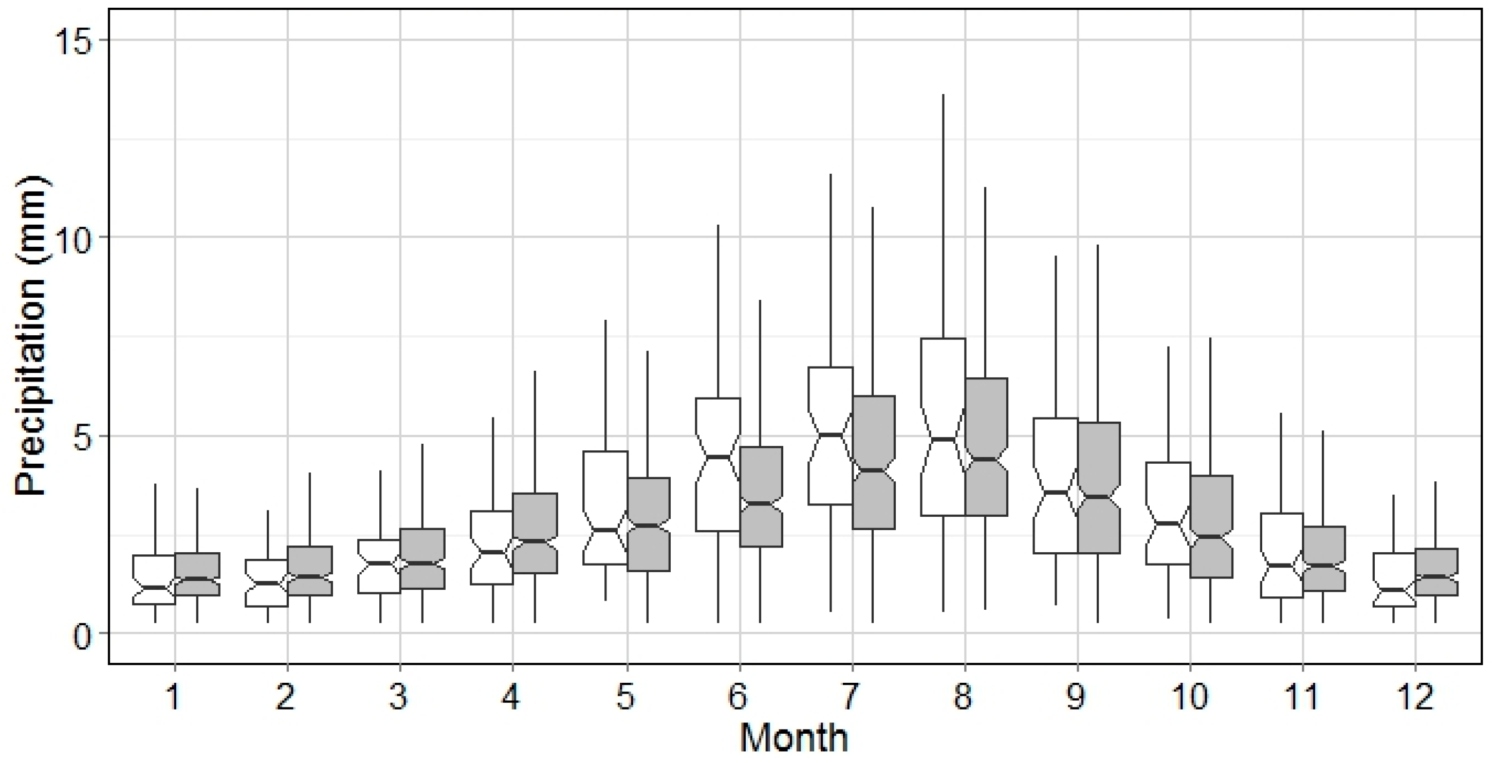
Figure 9, Figure 10 and Figure 11 further explore WEP results categorized by WED. Figure 9 focuses on WEP for WED > 10 h and shows that the summer and fall monthly average WEP are higher than those of the other seasons, and also have greater variability. The 95% confidence interval notch areas associated with the observations and predictions generally overlap with only slight deviations in April, May, and November. The mean WEP for all months is approximately 25 mm. WEPs for 5 h < WED < 10 h are approximately 10 mm, as shown in Figure 10. Seasonality is more evident in this range with significant differences occurring in August. The WEPs for short WED less than or equal to 5 h (Figure 11) present monthly mean WEP peaks in summer and valleys in winter, similar to that of the 5–10 h category in Figure 10. The months of June and July are more variable. The monthly average WEP for this category is on the level of 3 mm.
3.2. Monthly Based Analysis for All Cities
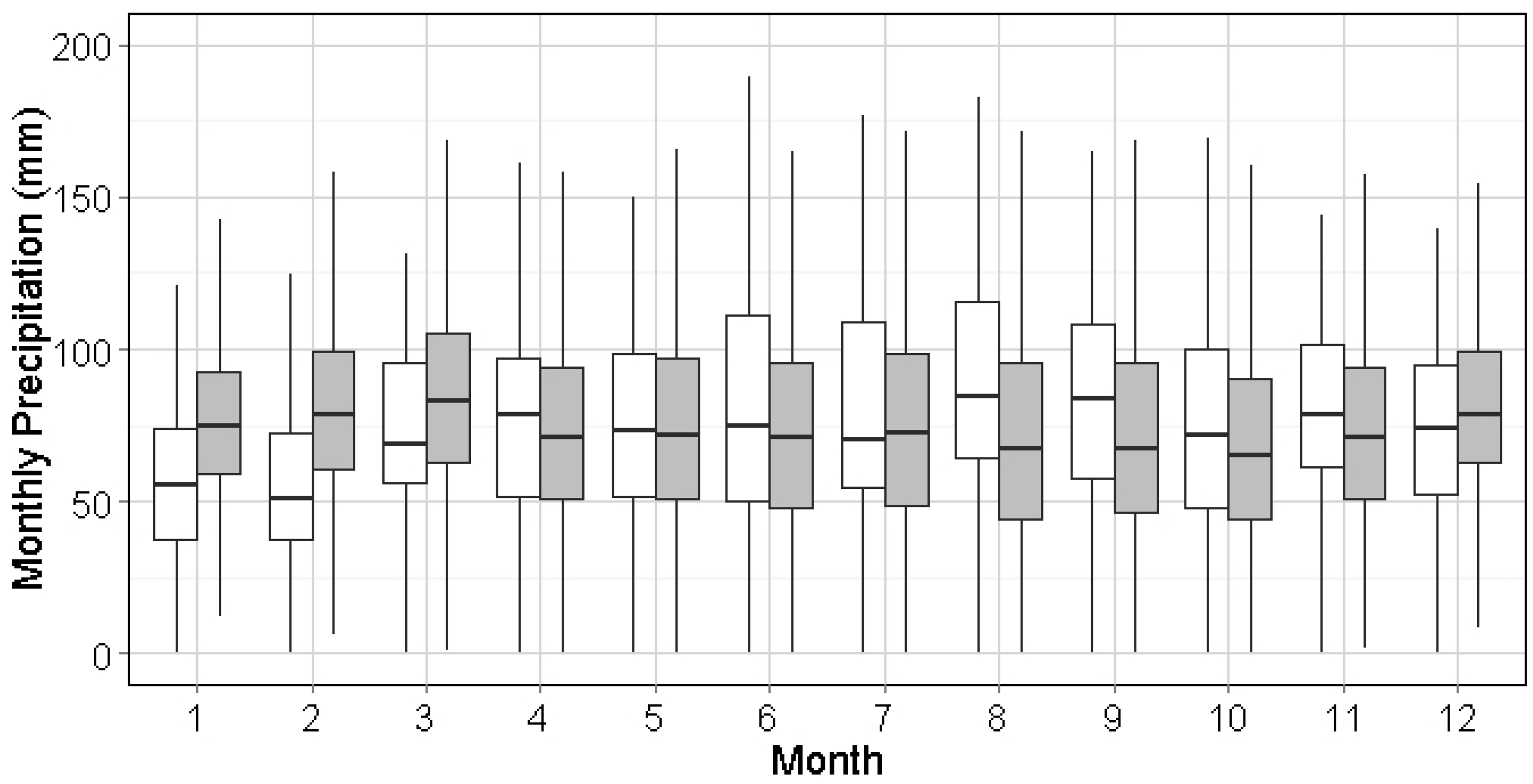
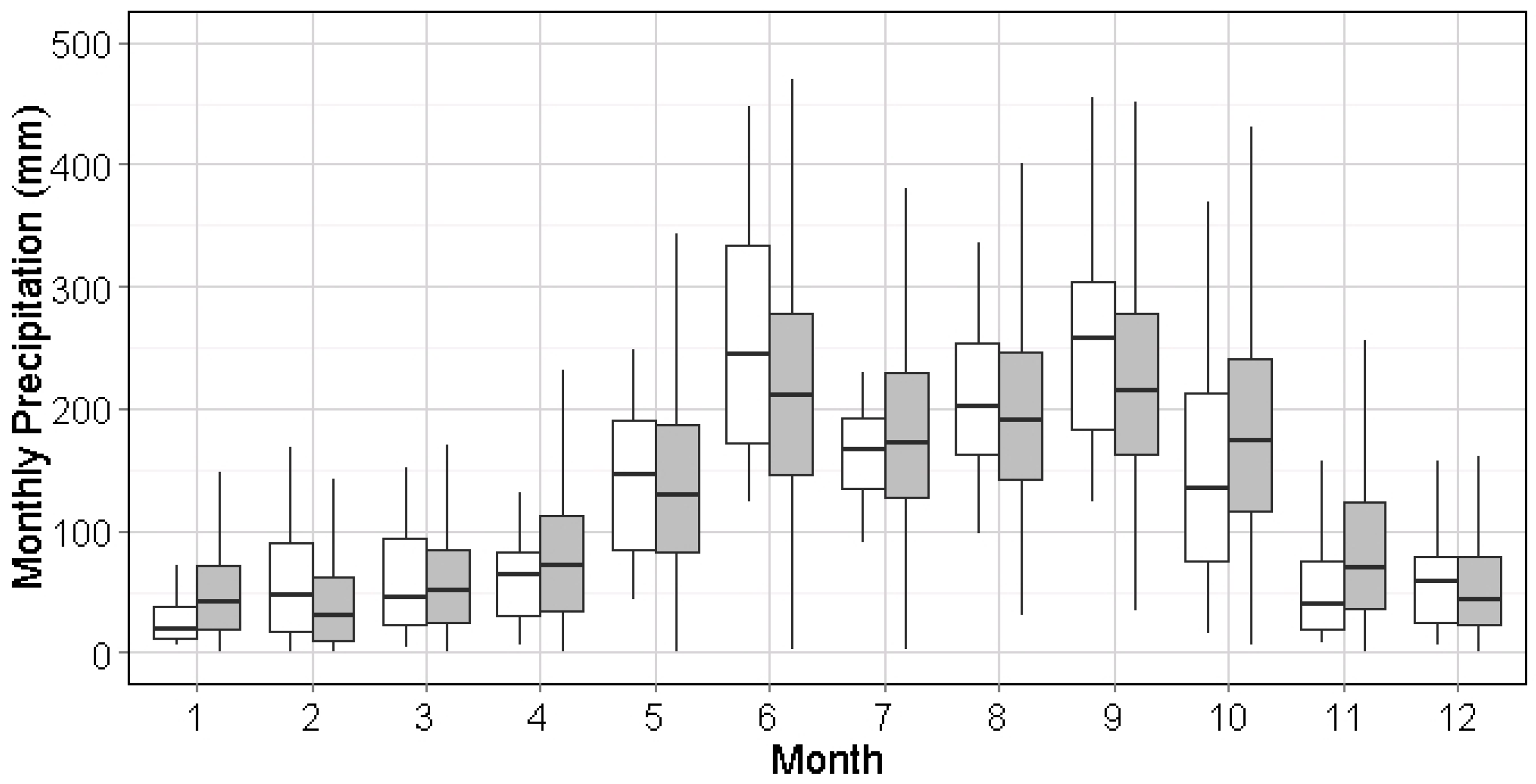
In order to demonstrate the portability of this algorithm, Figure 12, Figure 13 and Figure 14 show the comparison of monthly precipitations between historical and synthetic series for NYC, Syracuse, and Miami. For all cities, the seasonality of monthly precipitation is correctly repeated by the synthetic results. Given that the moving window algorithm has the feature of smoothing seasonality, fluctuation of monthly precipitation may be mitigated. Some relatively big differences are observed in July for NYC, January and February for Syracuse, and November for Miami.
4. Discussion
Generally, this algorithm was found to replicate the stationary distribution of precipitation for each month in all cities. Due to the design of the generation process, the moving window method preserves and smooths the seasonality of precipitation with two implications. First, the synthetic precipitation series may have a smoother seasonal shifting period than the historical record, as seen in May in Figure 6 and Figure 7. Next, the fluctuation of precipitation in synthetic series for each season (e.g., wet or dry) could be more stable in both mean and variation, i.e., January–March in Figure 13 and June–September in Figure 14. This indicates that the seasonal impact on hydrology in further calculations could be mitigated by using the synthetic series, which might be more obvious in the cities with significant seasonal difference, such as Miami, FL.
The alignment between the synthetic time series and the historical series in terms of the WEP can be interpreted by local atmospheric circulation patterns. In Figure 8, the variation of mean WEP in NYC is narrower in winter and spring than in summer and fall. The spring period coincides with when the jet stream moves northward, producing a high frequency of drizzles. By contrast, intensive air convections generating thunderstorms and hurricanes are more popular from July–November.
The general pattern of wet events for all months is demonstrated by integrating the analysis of WED and WEP. Based on Figure 6, the hot season and cold season is divided by the WED of 5 h. This implies that the WEP analysis can be interpreted categorically, e.g., WED > 10 h (Figure 9), WED between 5 h and 10 h (Figure 10), and those with WED < 5 h (Figure 11). It could be seen from Figure 9, Figure 10 and Figure 11 that the WEP range increases as the wet event gets longer. Biggest WEP variations can be observed from July–August, which indicates the precipitation intensity in summer season is much higher. However, this is not seen in Figure 8 because a big portion of wet events in summer are of short WED (Figure 4), i.e., thunder storms. Weighted by the portion of each WED category, the variation of WEP in summer season is mainly contributed by events of WED < 5 h with relatively low WEP. In contrast, WED in October is, on average, longer than 5 h, and the WEP variation is largest in October, as shown in Figure 8.
The potential for bias in runoff calculations may come from dry events. Does the algorithm resample short, dry events more frequently so that the soil moisture drying process isn’t as complete as it should be? For example, in NYC, the variability in DED is relatively large compared to WED. The SD of WED is about 6 h; by contrast the SD for DED is about 75 h. This indicates that, generally, the synthetic dry event would not significantly impact the accuracy of urban runoff simulations as the soil moisture drops most rapidly in the first 24-hours after a wet event, after which the drying process is significantly slowed and has minimum impact on stormwater runoff calculations.
Potential Improvement
This paper is a first from a big project investigating potential climate change uncertainties and their impact on green infrastructure (GI) performance in urban watershed. The focus of this study was to test if non-parametric precipitation generation could preserve the stationarity of precipitation using a single variable. Although that was demonstrated in this paper, there still exists some uncertainty on the future applications of this method in urban hydrology practice. These uncertainties include the need to develop a generalized means of determining IntEDP, assessing the reliability of using non-stationary methods to predict regionalized precipitation from a limited sample record, and the non-stationary impacts of climate change and local and temporal variation in weather patterns. Companion papers and future work on this big project will be used to fill in these gaps.
The IntEDP in this study is defined with qualitative evidence. Ideally, a sensitivity analysis is needed to discover a value that preserves the statistic consistency. However, such a value is highly localized, and the process to develop a generalized value for a wider application is complex. The purpose of showing Figure 1 is to provide a simple guide for non-expert users to determine a value for their own applications. A companion paper, Yu, Miller [34], has introduced a generalized method based on Reference [36].
The representativeness of the precipitation models is highly dependent on the sample size of the historical records, which is an inherent weakness when modeling two common scenarios in urban hydrology: Rare events and short observation records. In different ways, both of these situations have a limited sample size that harms the resampling process. For parametric stochastic methods, Bárdossy [37] suggested a simulated annealing process to incorporate the regional precipitation properties into a model. Pinault and Allier [38] extended the stochastic precipitation results into a catchment scale by keeping the spatial distribution consistency. Yet, neither method applies to a non-parametric model, which is highly data driven. One possible solution would be to lump observations from several nearby locations with similar climates to expand the feeding sample. For example, Yu, Miller [34] investigated the general relationship between precipitation and temperature at an hourly scale by combining the data from NYC, Philadelphia, and Boston. Such a solution would increase the geographic area represented by the synthetic ensembles and allow for more widespread use.
Precipitation dynamics under the effects of climate change and/or general climate variability, including temporally varying basins [39], may violate the stationarity assumptions of the non-parametric method. However, meteorological dynamics are a complex process that cannot be represented by traditional stochastic-based methods relying on only precipitation data. Unless one digs into the physical basis of the formation of precipitation with other variables, “How does precipitation vary on temperature, time and geography?” is hard to be unfold. This is also an extension topic of this research. Yu, Miller [34] have associated hourly precipitation and monthly temperature mediated by pressure change, which is the direct cause of cloud and precipitation formation. Another study that applies this finding to a non-stationary precipitation generator for climate change using similar stochastic methods on multi-dimensional data has been completed and will be published soon. In fact, this model may also apply to regionalized precipitation when importing the necessary climate variables from other locations without considering climate change, because the physical concept of precipitation formation holds regardless of location. In addition, this addition paper explores the Clausius–Clapeyron relation, used by many researchers in precipitation change under global warming, which is useful for predicting extreme events.
5. Summary and Conclusions
This paper describes the development of a non-parametric approach for stationary, synthetic, hourly precipitation generation. KNN methods, coupled with a moving-window theory, were employed to estimate the sequence of a state-change based on the current calendar day. Ultimately these stochastic results are representative of the historic record in terms of the aggregate monthly total precipitation, event duration, and event precipitation statistics.
The algorithm developed here was used to simulate hourly precipitation for NYC, Syracuse, and Miami based on more than 50 years of observations. The algorithm was able to simulate observed seasonality and historic distribution characteristics for event-based duration and precipitation. The results proved that the synthetic ensembles are representative of the historic record and the methods are transferable to multiple locations.
Author Contributions
Z.Y., F.M. and U.L. conceptualized the methodology; Z.Y. conducted the programming, data visualization and formal analysis; F.M. and Z.Y. validated the results; Z.Y. prepared the original draft; S.M. and F.M. reviewed and edited the manuscript; F.M. also supervised the project and acquired the research funding. All authors read and approved the manuscript.
Funding
This research was supported by the National Oceanic and Atmospheric Administration (NOAA) Supporting Regional Implementation of Integrated Climate Resilience: Consortium for Climate Risks in the Urban Northeast (CCRUN) Phase II* (NA15OAR4310147).
Acknowledgments
We thank many colleagues from Drexel University and Columbia University for the insights and expertise they provided which greatly assisted in this research. We also thank for the reviewers’ comments that greatly improved the manuscript.
Conflicts of Interest
The authors declare no conflict of interest.
References
- Dubrovský, M.; Buchtele, J.; Žalud, Z. High-frequency and low-frequency variability in stochastic daily weather generator and its effect on agricultural and hydrologic modelling. Clim. Chang. 2004, 63, 145–179. [Google Scholar] [CrossRef]
- Acharya, N.; Frei, A.; Chen, J.; DeCristofaro, L.; Owens, E.M. Evaluating stochastic precipitation generators for climate change impact studies of New York City’s primary water supply. J. Hydrometeorol. 2017. [Google Scholar] [CrossRef]
- Efstratiadis, A.; Dialynas, Y.G.; Kozanis, S.; Koutsoyiannis, D. A multivariate stochastic model for the generation of synthetic time series at multiple time scales reproducing long-term persistence. Environ. Model. Softw. 2014, 62, 139–152. [Google Scholar] [CrossRef]
- Haberlandt, U.; von Eschenbach, A.D.E.; Buchwald, I. A space-time hybrid hourly rainfall model for derived flood frequency analysis. Hydrol. Earth Syst. Sci. 2008, 12, 1353–1367. [Google Scholar] [CrossRef] [Green Version]
- Basinger, M.; Montalto, F.; Lall, U. A rainwater harvesting system reliability model based on non-parametric stochastic rainfall generator. J. Hydrol. 2010, 392, 105–118. [Google Scholar] [CrossRef]
- Shamir, E.; Megdal, S.B.; Carrillo, C.; Castro, C.L.; Chang, H.-I.; Chief, K.; Corkhill, F.E.; Eden, S.; Georgakakos, K.P.; Nelson, K.M.; et al. Climate change and water resources management in the Upper Santa Cruz River, Arizona. J. Hydrol. 2015, 521, 18–33. [Google Scholar] [CrossRef] [Green Version]
- Wilks, D.S.; Wilby, R.L. The weather generation game: A review of stochastic weather models. Prog. Phys. Geogr. 1999, 23, 329–357. [Google Scholar] [CrossRef]
- Cârsteanu, A.; Foufoula-Georgiou, E. Assessing dependence among weights in a multiplicative cascade model of temporal rainfall. J. Geophys. Res. Atmos. 1996, 101, 26363–26370. [Google Scholar] [CrossRef]
- Eagleson, P.S. Dynamics of flood frequency. Water Resour. Res. 1972, 8, 878–898. [Google Scholar] [CrossRef]
- Koutsoyiannis, D.; Pachakis, D. Deterministic chaos versus stochasticity in analysis and modeling of point rainfall series. J. Geophys. Res. Atmos. 1996, 101, 26441–26451. [Google Scholar] [CrossRef]
- Rodriguez-Iturbe, I.; Gupta, V.K.; Waymire, E. Scale considerations in the modeling of temporal rainfall. Water Resour. Res. 1984, 20, 1611–1619. [Google Scholar] [CrossRef]
- Neyman, J.; Scott, E.L. Statistical approach to problems of cosmology. J. R. Stat. Soc. Ser. B (Methodol.) 1958, 20, 1–43. [Google Scholar] [CrossRef]
- Rodriguez-Iturbe, I.; Cox, D.R.; Isham, V. Some models for rainfall based on stochastic point processes. Proc. R. Soc. Lond. Ser. A. Math. Phys. Sci. 1987, 410, 269–288. [Google Scholar] [CrossRef]
- Rodriguez-Iturbe, I.; Cox, D.R.; Isham, V. A point process model for rainfall: Further developments. Proc. R. Soc. Lond. Ser. A. Math. Phys. Sci. 1988, 417, 283–298. [Google Scholar] [CrossRef]
- Wilks, D.S. Multisite generalization of a daily stochastic precipitation generation model. J. Hydrol. 1998, 210, 178–191. [Google Scholar] [CrossRef]
- Stern, R.D.; Coe, R. A model fitting analysis of daily rainfall data. J. R. Stat. Soc. Ser. A. (Gen.) 1984, 147, 1–34. [Google Scholar] [CrossRef]
- Wasko, C.; Pui, A.; Sharma, A.; Mehrotra, R.; Jeremiah, E. Representing low-frequency variability in continuous rainfall simulations: A hierarchical random Bartlett Lewis continuous rainfall generation model. Water Resour. Res. 2015, 51, 9995–10007. [Google Scholar] [CrossRef] [Green Version]
- Wasko, C.; Sharma, A. Continuous rainfall generation for a warmer climate using observed temperature sensitivities. J. Hydrol. 2017, 544, 575–590. [Google Scholar] [CrossRef]
- Islam, S.; Entekhabi, D.; Bras, R.L.; Rodriguez-Iturbe, I. Parameter estimation and sensitivity analysis for the modified Bartlett-Lewis rectangular pulses model of rainfall. J. Geophys. Res. Atom. 1990, 95, 2093–2100. [Google Scholar] [CrossRef]
- Entekhabi, D.; Rodriguez-Iturbe, I.; Eagleson, P.S. Probabilistic representation of the temporal rainfall process by a modified Neyman-Scott Rectangular Pulses Model: Parameter estimation and validation. Water Resour. Res. 1989, 25, 295–302. [Google Scholar] [CrossRef] [Green Version]
- Burlando, P.; Rosso, R. Comment on “Parameter estimation and sensitivity analysis for the modified Bartlett-Lewis rectangular pulses model of rainfall” by S. Islam et al. J. Geophys. Res. Atom. 1991, 96, 9391–9395. [Google Scholar] [CrossRef]
- Rajagopalan, B.; Salas, J.D.; Lall, U. Stochastic methods for modeling precipitation and streamflow. In Advances in Data-Based Approaches for Hydrologic Modeling and Forecasting; World Scientific: Singapore, Singapore, 2010; pp. 17–52. [Google Scholar]
- Rodriguez-Iturbe, I.; Febres De Poweret, B.; Sharifi, M.B.; Georgakakos, K.P. Chaos in rainfall. Water Resour. Res. 1989, 25, 1667–1675. [Google Scholar] [CrossRef]
- Scott, D.W. Multivariate Density Estimation: Theory, Practice, and Visualization; Wiley: Hoboken, NJ, USA, 2015. [Google Scholar]
- Silverman, B.W. Density Estimation for Statistics and Data Analysis; Chapman and Hall: London, UK, 1986. [Google Scholar]
- Efron, B.; Tibshirani, R.J. An Introduction to the Bootstrap; Chapman and Hall: New York, NY, USA, 1994. [Google Scholar]
- Lall, U.; Sharma, A. A nearest neighbor bootstrap for resampling hydrologic time series. Water Resour. Res. 1996, 32, 679–693. [Google Scholar] [CrossRef]
- Sharif, M.; Burn, D.H.; Wey, K. Daily and hourly weather data generation using a K-nearest neighbour approach. In Proceedings of the 18th CSCE Canadian Hydrotechnical Conference, Winnipeg, MB, Canada, 22–24 August 2007. [Google Scholar]
- Sharif, M.; Burn, D.H. Improved K-nearest neighbor weather generating model. J. Hydrol. Eng. 2007, 12, 42–51. [Google Scholar] [CrossRef]
- Sharma, A.; Lall, U. A non-parametric approach for daily rainfall simulation. Math. Comput. Simul. 1999, 48, 361–371. [Google Scholar] [CrossRef]
- Rajagopalan, B.; Lall, U. A k-nearest-neighhor simulator for daily precipitation and other weather variables. Water Resour. Res. 1999, 35, 3089–3101. [Google Scholar] [CrossRef]
- Rajagopalan, B.; Lall, U.; Tarboton, D.G. Nonhomogeneous Markov model for daily precipitation. J. Hydrol. Eng. 1996, 1, 33–40. [Google Scholar] [CrossRef]
- Lall, U.; Rajagopalan, B.; Tarboton, D.G. A non-parametric wet/dry spell model for resampling daily precipitation. Water Resour. Res. 1996, 32, 2803–2823. [Google Scholar] [CrossRef]
- Yu, Z.; Miller, S.; Montalto, F.; Lall, U. The bridge between precipitation and temperature–Pressure Change Events: Modeling future non-stationary precipitation. J. Hydrol. 2018, 562, 346–357. [Google Scholar] [CrossRef]
- Chambers, J.M. Graphical Methods for Data Analysis; Chapman and Hall/CRC: New York, NY, USA, 1983. [Google Scholar]
- Restrepo-Posada, P.J.; Eagleson, P.S. Identification of independent rainstorms. J. Hydrol. 1982, 55, 303–319. [Google Scholar] [CrossRef]
- Bárdossy, A. Generating precipitation time series using simulated annealing. Water Resour. Res. 1998, 34, 1737–1744. [Google Scholar] [CrossRef]
- Pinault, J.-L.; Allier, D. Regionalization of rainfall for broad-scale modeling: An inverse approach. Water Resour. Res. 2007, 43, W09422. [Google Scholar] [CrossRef]
- Thirel, G.; Andréassian, V.; Perrin, C.; Audouy, J.-N.; Berthet, L.; Edwards, P.; Folton, N.; Furusho, C.; Kuentz, A.; Lerat, J.; et al. Hydrology under change: An evaluation protocol to investigate how hydrological models deal with changing catchments. Hydrol. Sci. J. 2015, 60, 1184–1199. [Google Scholar] [CrossRef]
Figure 1.
IntEDP analysis for Miami, NYC, and Syracuse.

Figure 2.
Non-parametric stochastic generator flow chart.

Figure 3.
Sample of K nearest neighbors (KNN) on precedent event condition.

Figure 4.
Boxplots of Wet Event Duration (WED) means (Historical: White, Synthetic: Grey).

Figure 5.
Boxplots of WED SDs (Historical: White, Synthetic: Grey).

Figure 6.
Boxplots of Dry Event Duration (DED) means (Historical: White, Synthetic: Grey).

Figure 7.
Boxplots of DED SDs (Historical: White, Synthetic: Grey).

Figure 8.
Boxplots of Wet Event Precipitation (WEP) means (Historical: White, Synthetic: grey).

Figure 9.
Boxplots of WEP means with WED longer than 10 h (Historical: White, Synthetic: Grey).

Figure 10.
Boxplots of WEP means with WED between 5 and 10 h (Historical: White, Synthetic: Grey).

Figure 11.
Boxplots of WEP means with WED less than 5 h (Historical: White, Synthetic: Grey).

Figure 12.
Comparison of monthly precipitation of synthetic series and historical observations in NYC (Historic: White, Synthetic: Grey).
Figure 12.
Comparison of monthly precipitation of synthetic series and historical observations in NYC (Historic: White, Synthetic: Grey).

Figure 13.
Comparison of monthly precipitation of synthetic series and historical observations in Syracuse (Historic: White, Synthetic: Grey).
Figure 13.
Comparison of monthly precipitation of synthetic series and historical observations in Syracuse (Historic: White, Synthetic: Grey).

Figure 14.
Comparison of monthly precipitation of synthetic series and historical observations in Miami (Historic: White, Synthetic: Grey).
Figure 14.
Comparison of monthly precipitation of synthetic series and historical observations in Miami (Historic: White, Synthetic: Grey).

© 2019 by the authors. Licensee MDPI, Basel, Switzerland. This article is an open access article distributed under the terms and conditions of the Creative Commons Attribution (CC BY) license (http://creativecommons.org/licenses/by/4.0/).
Share and Cite
MDPI and ACS Style
Yu, Z.; Miller, S.; Montalto, F.; Lall, U. Development of a Non-Parametric Stationary Synthetic Rainfall Generator for Use in Hourly Water Resource Simulations. Water 2019, 11, 1728. https://doi.org/10.3390/w11081728
AMA Style
Yu Z, Miller S, Montalto F, Lall U. Development of a Non-Parametric Stationary Synthetic Rainfall Generator for Use in Hourly Water Resource Simulations. Water. 2019; 11(8):1728. https://doi.org/10.3390/w11081728
Chicago/Turabian StyleYu, Ziwen, Stephanie Miller, Franco Montalto, and Upmanu Lall. 2019. "Development of a Non-Parametric Stationary Synthetic Rainfall Generator for Use in Hourly Water Resource Simulations" Water 11, no. 8: 1728. https://doi.org/10.3390/w11081728
Note that from the first issue of 2016, this journal uses article numbers instead of page numbers. See further details here.