Hydrodynamic Drivers of Dissolved Oxygen Variability within a Tidal Creek in Myrtle Beach, South Carolina
by

Douglas M. Pastore
1, 
Richard N. Peterson
1,
Diane B. Fribance
2,
Richard Viso
1 and
Erin E. Hackett
1,* 1
Department of Coastal and Marine Systems Science, Coastal Carolina University, Conway, SC 29528, USA
2
Department of Marine Science, Coastal Carolina University, Conway, SC 29528, USA
*
Author to whom correspondence should be addressed.
Water 2019, 11(8), 1723; https://doi.org/10.3390/w11081723
Submission received: 17 June 2019
/
Revised: 14 August 2019
/
Accepted: 15 August 2019
/
Published: 19 August 2019
(This article belongs to the Section Water Quality and Contamination)
Abstract
:Beach erosion and water quality degradation have been observed in Singleton Swash, a tidal creek that traverses the beach-face connecting land and ocean in Myrtle Beach, SC. The objective of this study in Singleton Swash is to explore relationships between water quality and hydrodynamics, where the latter are influenced by beach face morphology. We measure water velocities, water levels, and dissolved oxygen concentrations (DO) (a proxy for water quality) and apply correlation analysis to examine the relationships between physical processes and dissolved oxygen variations. Results show that larger tidal ranges are associated with higher mean levels of DO in the tidal creek. The larger tidal ranges are linked to larger magnitude currents, which increase both the DO transport via larger fluxes of oxygenated oceanic water into the swash and the magnitude of Reynolds shear stresses; due to tidal asymmetries, flood currents are stronger than ebb currents in this system. Based on these results, it is concluded that the combined transport of oxygenated waters into the tidal creek from the ocean on large flood tides and subsequent mixing due to large Reynolds shear stresses result in the observed net DO concentration increases in the creek over tidal cycles.
1. Introduction
Tidal creeks are common along the southeastern coast of the United States and serve many functions for the surrounding ecosystem and infrastructure. Tidal creeks also act as conduits to connect terrestrial and coastal marine systems, often promoting growth and development of extensive salt marsh ecosystems along their flow paths. The abundance of sediment along the southeast coastline (both inland and in the coastal ocean) allows for continued marsh surface accretion, which dictates the level of inundation of flora and fauna throughout daily tidal cycles within these systems [1,2]. A change in inundation and mean-sea level can impact species distribution due to changes in local habitat [1], which may in turn influence the overall function and health of tidal creek systems.
Tidal creek systems are highly susceptible to change due to variations in tidal forcing. Sediment supply and solute concentration are among the factors that vary with tides, local winds, non-tidal currents, and waves [3]. Anthropogenic modifications to these systems (e.g., dredging, construction, and runoff alteration) can also change the tidal creek system both directly and indirectly. Runoff alteration via engineered conveyance systems, for example, can change drainage characteristics and affect natural flow dynamics between tidal creeks and the ocean, which may, in turn, affect biogeochemical cycling and ecosystem function.
Natural processes such as sediment deposition can restrict tidal exchange in these systems. Restricted exchange can decrease water velocities in the creek, enabling salinity stratification that limits vertical mixing of oxygen into and within the water column, thus leading to impaired water quality conditions. Reduced mixing and transport of dissolved oxygen (DO) and other solutes (e.g., nutrients) can stress local organisms due to low supply of these life-sustaining compounds, thus degrading overall ecosystem health [4].
This study focuses on Singleton Swash, a typical tidal creek located 11 km north of Myrtle Beach, South Carolina (Figure 1A). Tides along the micro-tidal coast are roughly 1.5 m, differing from the ~0.5 m tidal range observed within Singleton Swash. The tidal creek extends approximately 2 km inland with an average depth and width of 0.75 m and 14 m, respectively. Channel cross-section geometry inland of the dynamic beach-face is approximately rectangular in shape exhibiting nearly vertical bank construction with respect to the channel bed. The path of the inland channel is highly stable due to dense vegetation, whereas the section of channel that traverses the beach-face is highly dynamic. The creek terminates inland at a fresh water pond that drains over a weir and into the swash basin. Along with drainage from the pond, a local golf course, salt marsh, and hotel/condominium development comprise the 6.8 km2 watershed [5].
Littoral drift causes the (beach-face portion of the) creek channel to migrate southward where it threatens local infrastructure. Water quality of the inland salt marsh also becomes degraded during periods of increased creek channel migration. Attempts to mitigate erosion and water quality degradation occur periodically (~every 8 months) by dredging and straightening the beach-face channel.
A previous study of Singleton Swash [5] suggests that beach-face morphology is associated with DO variations within the creek channel. Stable salinity stratification within the creek was found to vary inversely with tidal range; presumably, reduced tidal ranges enable setup of salinity stratification due to reduced vertical mixing, which would also limit mixing of DO. In Hoffnagle [5], tidal range was used as a proxy for flushing, but no clear relationship between DO concentration and salinity stratification could be established to verify the aforementioned presumption. Consequently, the author notes the need for more research to understand the mechanics of dissolved oxygen exchange and transport within the creek system.
This study thus aims to evaluate the effect of hydrodynamics on water quality variability within the Singleton Swash tidal creek system. Specifically, here, we seek to establish general trends in relationships between hydrodynamic parameters and water quality, where we use DO as a proxy for water quality. Understanding these relationships between hydrodynamic parameters and DO enables insight into how variations in beach-face morphology may impact water quality in the swash because prior studies have examined linkages between these morphologies and hydrodynamic proxies (i.e., tidal range) [5]. Observations of water level, water velocities, and derived mixing indicators within the tidal creek provide insight into the relative role of these mechanisms in driving water quality changes. Correlation analysis is used to explore the (leading order linear) relationships between hydrodynamic and water quality variables by establishing the type, significance, and temporal scale at which any relationships occur. The results of this study provide insight into tidal forcing, mixing and DO dynamics within nearshore tidal creeks common in the southeastern U.S., and in connection with Hoffnagle [5], can provide insights linking beach-face morphology and water quality through the hydrodynamics of such systems.
2. Field Observations
Measurements were performed at three locations as illustrated in Figure 1B: (i) at Site A; (ii) at Site B (160 m upstream of Site A); and (iii) at Site C (350 m upstream of Site A). Sites A and C are long-term monitoring stations in Singleton Swash that were leveraged for this study, and Site B was added for this study to measure additional hydrodynamic parameters that were not measured at the other sites. Site B was chosen because it is located between the other two sites in a straight section of the channel. Pressure sensors at Sites A and C (Onset Hobo Water Level Loggers) measured absolute pressure on 15-min intervals with an accuracy of 0.62 kPa (~0.5 cm of head) from 1 September 2017 through 1 June 2018. The sensors were deployed in PVC (polyvinyl chloride) pipe housings at Sites A and C approximately 0.3 and 0.1 m above the creek bed, respectively. Concurrent sea level barometric pressure measurements made approximately 1 km north of Site C are used to convert these pressure measurements to water levels. Water level was measured at Site B on 1-s intervals in May 2018 by a Nortek Vector at approximately 0.83 m above the creek bed with an accuracy of 0.05 m.
Water velocity was measured at Site B (1–31 May 2018) by a Nortek Vector acoustic Doppler velocimeter (ADV). The Vector was mounted onto a PVC frame drilled into the channel bed “facing down”, seen in Figure 2. The sample volume was located 15 cm below the probe head (approximately 56.5 cm above the creek bed, which is near mid-water column at high tide). The ADV measured three velocity components, u, v, and w corresponding to velocities in the along-channel (x), across-channel (y), and vertical (z) directions, respectively. Positive along-channel velocities are directed out of the creek into the ocean (downstream) and negative along-channel velocities are directed into the creek from the ocean (upstream). A nominal velocity range ±1.00 m/s (vertical = ±0.6 m/s, horizontal = ±2.1 m/s) was used to minimize Doppler noise in the measurements without water velocities exceeding this range. The Vector is accurate within ±0.5% of the measured velocity (or ±1 mm/s, whichever is greater).
Water velocities were measured at a frequency of 64 Hz over 5-min periods every 15 min to capture rapid change in tidal currents and resolve turbulent timescales [6]. Turbulent fluctuations are defined as deviations from the burst mean velocity (5 min average) in the absence of waves. Data were screened for wave-induced motion using fast Fourier transforms; bursts showing wave-induced flow were excluded from estimates of turbulence fluctuations to avoid wave contamination of Reynolds stress estimates [7,8,9].
Wind speeds were measured every 5-min by a meteorological station (Viasala WXT-536) located on a nearby pier (Apache pier). Wind speed measurements are utilized as an indicator of wind stress magnitude at the water surface, which is proportional to the square of wind speed [10].
Dissolved oxygen concentrations within Singleton Swash were measured continuously using an Onset HOBO Dissolved Oxygen Data Logger at Site A (1 September 2017 through 1 June 2018) and Site B (May 2018). DO concentration (mg/L) and temperature (°C) were measured at 5-min intervals with accuracies of ±0.2 mg/L and ±0.2 °C, respectively. At Site A, the DO probe was attached approximately 30 cm above the seabed to a PVC pipe anchored to the seabed. At Site B, the probe was similarly installed at 56.5 cm above the seabed (the same water-column location as the Vector’s sample volume). On a bi-weekly basis, the sensors were recovered for cleaning and corrected for drift using DO measurements performed with a YSI (Yellow Springs Instrument) ProODO.
3. Analytical Methods
3.1. Quality Control
The ADV data are filtered for erroneous values based on the correlation coefficients for pulse pairs of scattered sound measured along each beam [11]. The threshold used was a correlation coefficient of 0.90; values falling below this threshold have been excluded from the data set. Along with signal correlation, data were screened for low (<8 dB) signal-to-noise ratios (SNR) [11]. Values < 8 dB indicate low concentrations of acoustic reflecting materials in the sample volume or water levels falling below the transducer head. No low SNR values were observed, and it is therefore assumed that the water level never fell below the sensor head. Velocity measurements exceeding ±3.5 standard deviations from the burst-mean velocity have also been removed from the data. The threshold of 3.5 standard deviations was determined by trial and error; this threshold removed any clear outliers without removing valid high/low velocities. Velocity data from a sample burst is shown in Figure 3A, where it is evident that cross-channel velocities are much smaller than along-channel velocities.
Dissolved oxygen measurements are corrected for any drift in the DO record using HOBOware® (v3.7.15, Onset Computer Corporation, Bourne, MA, USA) and the calibration DO measurements made with the YSI. These corrections were performed bi-weekly with calibration DO measurements taken at the start and end interval. Additionally, consecutive DO percent saturation measurements differing by more than 20% were considered erroneous and removed from the data set. This threshold removed clear outliers within the time series.
Water level data were also screened for erroneous measurements by removing values that varied more than 0.5 m between consecutive measurements. This procedure assumes that, within a 15-min time period, the water level does not vary by more than 33% of the normal tidal range in the Grand Strand region (mean tidal range of 1.5 m) [12].
3.2. Tidal Range, Currents, and Discharge
A time series of tidal range is computed by subtracting consecutive high (maximum) and low (minimum) water levels. Times of high and low water levels are determined using , where is the temporal derivative of the water level time series. A zero phase-shift boxcar filter (two hour) was applied to the measured water level time series to reduce the effects of noise in determining the timing of zero-crossings. Tidal range time series for Site A was also low pass filtered with a (zero phase-shift) moving average filter of 14 days (removing the spring-neap cycle), and then linearly interpolated to a 14-day sampling interval. These filters were applied for Site A because it is used to examine long-term trends in water level within the tidal creek (see Section 4).
Discharge is computed from cross-sectional area of the channel at Site B and the current velocity as measured by the Vector. The cross-sectional area is calculated over the distance between the right (oceanic) bank and left (inland) banks [13,14]:
where the subscripts (BR and BL) indicate the position of the right (oceanic) and left (inland) banks, respectively, and is time. Water depth is a function of both cross-channel position and time. The depth of the channel for various y positions was measured manually and these values are adjusted based on the water height measurements made by the Vector. When water level fell below the pressure sensor, the depth was assumed to be 0.83 m (the location of the sensor). This assumption is reasonable as the water level did not fall below the Vector’s transducer head and the distance between the transducer head and pressure sensor is 0.15 m; thus, any difference in water depth from 0.83 m is minimal.
Cross-sectional area is used to determine the flood and ebb discharge (Qf and Qe), calculated over the rising and falling tides, respectively. Current velocity, , measured by the Vector at Site B, is the mean of the measured velocities over a burst-interval (i.e., 5-min) and is assumed to be homogeneous over the cross-section when computing discharge.
3.3. Reynolds Shear Stress
To characterize turbulent quantities within the creek, velocities measured by the ADV were decomposed as follows [8,15]:
where the prime denotes turbulent fluctuations. Wave-induced velocities are assumed to be negligible; therefore, bursts that were not consistent with this assumption were excluded from the data set to avoid wave contamination of Reynolds stresses [7].
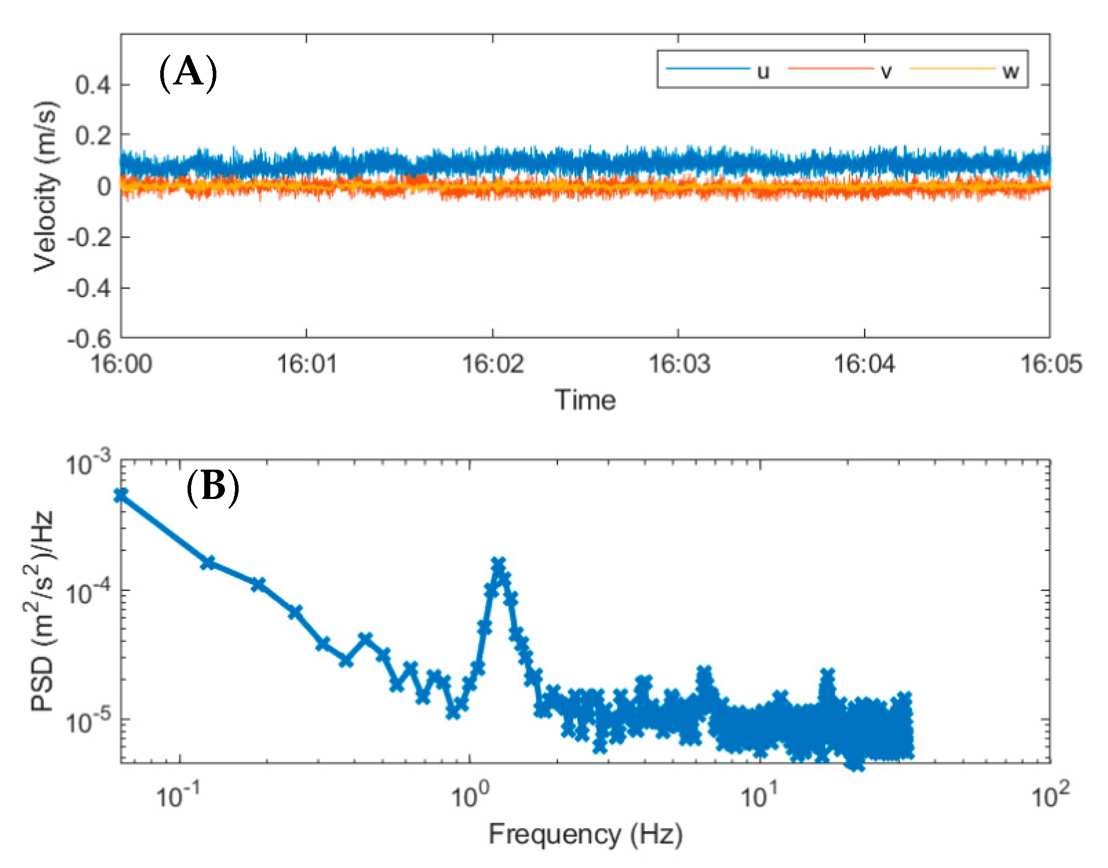
Spectral analysis using fast Fourier transforms of the along-channel velocity reveals the presence of wave velocities [16]. Welch’s method is used to calculate the power spectral density—each velocity time series burst was first de-trended, then sectioned into 1024 data points (16 s) with 50% overlap between adjacent sections. A Hamming window was applied over the sectioned data to reduce spectral leakage. Power spectral density was then estimated for each section and subsequently averaged over all sections to reduce noise. Spectral peaks that indicate variability in water velocity at frequencies corresponding to wave orbital velocities (approximately 0.1–1 Hz) are visually identified as wave contaminated bursts. An example of a burst with significant wave-induced motion is shown in Figure 3. Of the 2880 bursts, 74 (~2.5%) were removed from the dataset due to exhibiting wave orbital motion.
3.4. Pearson Correlation Analysis
The Pearson correlation coefficient (R) is computed as a function of discrete lag [17]:
where is discrete lag, is the number of discrete samples, the overbar denotes time series average, and the two variables being cross-correlated are and This technique quantifies the type of relationship (direct, inverse, or none), the strength of the relationship, and any lag between variables and . High correlation at a positive lag indicates that variability in precedes the variability in whereas negative lag indicates variability in follows variability in Correlations between various time series are performed in this study (Table 1). A 95% confidence interval is calculated for each correlation calculation to assess the significance of the correlation coefficient; correlation coefficients with confidence intervals that do not encompass zero are considered to denote significant relationships. Summaries of results of the correlation analysis are shown in Table 2.
4. Results and Discussion
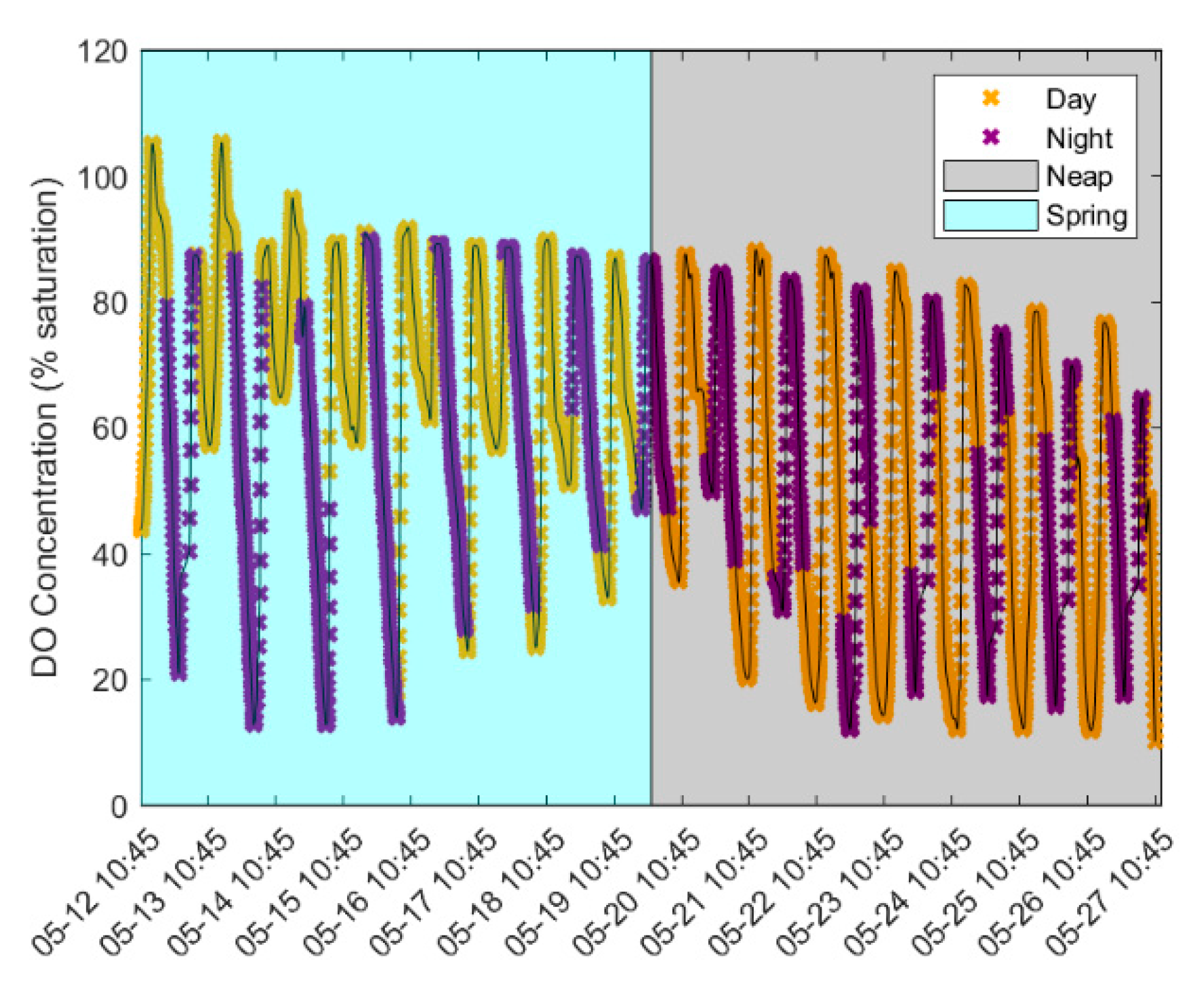
Dissolved oxygen concentration varies over both solar and tidal cycles as illustrated in Figure 4 (verified with a Fourier transform, not shown). Net autotrophy (photosynthesis) occurs during daylight hours, which increases DO concentration within the water column, and net heterotrophy (respiration) occurs during dark hours, which decreases DO concentrations. Periods of greatest DO saturation were observed when flood tides occurred simultaneously with hours of maximum sunlight. These periods were almost always proceeded by hypoxic conditions when DO concentrations were below 20% saturation.
Figure 4 demonstrates times of concurrent flood/daylight and ebb/night events. On 12 and 13 May, two periods of super-saturation (over 100%) were followed by very low DO concentrations (<~20% saturation). On these days, a high tide occurred during mid-day hours (2:00 p.m.–3:00 p.m.) and low tides occurred during night hours (12:00 a.m.–1:00 a.m.). Over the course of the time series shown in Figure 4, the opposite scenario also occurs—for example, on 19–20 May, when a high tide took place during nighttime. In this case, we observe a narrow range in DO concentration over a day, implying removal of oxygen due to net heterotrophy was offset by a supply of oxygen from a flood tide, which resulted in a reduced range of daily DO concentrations. The day/night DO variability suggests biological mechanisms influence DO concentration but increases in DO observed during the nighttime hours suggest that hydrodynamic mechanisms are also significant. This paper focuses on the hydrodynamic mechanisms forcing DO variations. Biologically forced DO variations within Singleton Swash are more thoroughly discussed in Hoffnagle [5] and Pastore [13].
For most of the study period, spring tides show higher mean DO concentration than neap tides, suggesting that larger tidal ranges increase the overall inventory of dissolved oxygen within the creek. During neap tides (grey shaded areas in Figure 4), lower maximum concentrations and a slightly decreasing mean DO concentration over tidal cycles support this observation. These differences between spring and neap tides also reflect the effects of the relative timing between tidal cycles and daily solar cycles. For example, during neap tides (19–27 May), higher maxima in DO concentration occurs when daylight hours and high tide coexist (yellow peaks); inversely, periods when high tide occurs at night show lower maxima DO concentrations (purple peaks).
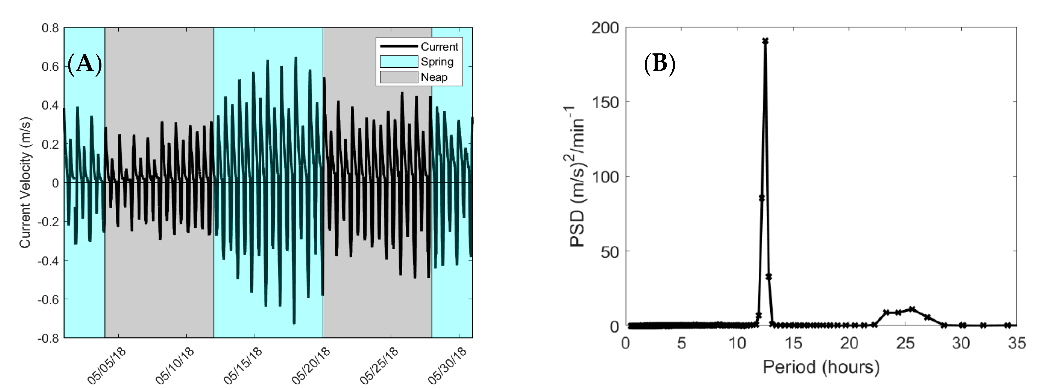
Figure 5A illustrates the observed along-channel current () during May 2018. Average flood and ebb current velocities observed throughout the deployment were 0.23 and 0.16 m/s, respectively. The difference between average flood and ebb tidal current velocity suggests tidal asymmetry within the swash. Average cross-channel currents () at the ADV measurement location over the deployment were on the order of 10−5 m/s and thus are considered negligible.
Tidal currents within Singleton Swash are asymmetric with higher magnitude velocities over shorter periods during flood tide. This result has been observed in similar estuarine systems [18,19] and is attributed to friction and time-variable channel cross-sectional area within a system. Water velocities also demonstrate a mixed semidiurnal tidal cycle, illustrated in Figure 5A. A similar, semidiurnal signal is observed in the ocean tides in this region. Figure 5B shows the spectral density of , with a dominant spectral peak occurring at a period of approximately 12.5 h denoting the influence of ocean tidal cycles within the creek. This influence from ocean tides indicates that water velocities within the creek are predominantly tidally driven. These conditions are observed in similar systems [20,21] and cause peak flood tidal velocities to exceed those during ebb tide, whereas ebb tide persists almost twice as long as flood tide. Lower spectral peaks (Figure 5B) are likely associated with the observed tidal asymmetry between flood and ebb, diurnal tides, and tidal harmonics.
Fluctuations in tidal velocity are concurrent with the periodicity in dissolved oxygen concentration. Average correlation between DO and over two-day intervals in May shows a significant inverse relationship (R = −0.511, 1.75-h lag; Table 2). As flood velocities are represented by negative values, an inverse relationship implies that DO saturation is high when flood currents are strong and low when ebb currents are strong. The approximate alignment of peak DO concentrations with peak flood currents supports this relationship, whereas the peak ebb currents precede DO minima, and slack low tide occurs simultaneously with DO concentration minima. These relationships suggest that current is an important factor in controlling DO concentrations in the creek. A lag in the correlation of DO and of approximately 1 h and 45 min indicates that variation in DO concentration occurs after a change in current velocity. Transport of DO saturated water into the creek occurs during flood tide with higher magnitude currents increasing saturation levels; inversely, ebb tides transport water with lower DO concentrations from the upstream salt marsh into the creek channel.
Tidal range has been linked to morphological and salinity gradients within Singleton Swash [5]. Results discussed in this study reveal distinct tidal signatures. Water level measurements have been conducted over a much longer time period than the deployment of the ADV, possibly allowing for the extrapolation of transport and mixing results over this period. For this extrapolation to be feasible, hydrodynamic characteristics must be linked to tidal range. To explore these connections, tidal range was correlated to each of the aforementioned physical processes through correlation analysis (Table 2). In Table 2, the time series resolution (CR) indicates either the sampling interval or the period of time the data were averaged prior to the correlation if CR is greater than the sampling interval. The data is segmented and correlated over each segment, then the correlation coefficients are averaged over all possible segments at each lag. This segment is referred to as the correlation time interval (CI) (Table 2).
Water level reveals spring-neap cyclicity as well as a semidiurnal tidal regime illustrated in Figure 5. Periods of large tidal range indicate spring tides while periods of low tidal range indicate neap tides at all sites, where tidal range fluctuates between 0.12 m and 0.88 m. The correlation of tidal range between Sites A and C from 1 September 2017 to 1 January 2018, shows consistent variation in tidal ranges throughout the creek (R = 0.987, 0 day-lag). Furthermore, a significant relationship exists between tidal range and both maximum flood (R = 0.927, 0 day-lag) and ebb (R = 0.842, 0 day-lag) tidal velocities. These results confirm that tidal range can be reliably used as a relative indicator of current velocity throughout this system.
A direct relationship between maximum flood current velocity and dissolved oxygen (R = 0.927, 0 h-lag) implicitly links DO concentration to tidal range. Correlation analysis between DO concentration and tidal range (CI = 14 days) from September 2017 through June 2018 reveals a weak but statistically significant relationship (R = 0.277, 1.5 day-lag). DO concentration was downsampled to a 12-h time interval (CR) to match the resolution of the tidal range time series. The CI of this DO concentration time series and tidal range captures variations in dissolved oxygen and tidal range occurring over timescales longer than a tidal cycle. A direct relationship with a lag of 1.5 days between tidal range and dissolved oxygen concentrations indicates that an increase in tidal range precedes an increase in DO concentration. This finding suggests higher tidal ranges result in a net increase in DO concentrations within the system over time.
Discharge was calculated over 114 tides (57 flood, 57 ebb) during the May deployment. Singleton Swash is ebb dominated with respect to discharge: despite stronger current velocity during flood tide, the prolonged ebb tidal periods discharge more water volume than enters during flood tide. The average ebb discharge per tidal cycle was 4.52 × 10⁵ m3 (total ebb discharge over May was 2.58 × 10⁷ m3) while the average flood discharge per tidal cycle was 9.97 × 10⁴ m3 (total flood discharge over May was 5.68 × 10⁶ m3). This result as well as the strong correlation between discharge and tidal range (R = 0.754 for flood Q; R = 0.977 for ebb Q) indicates that the creek system is not storing water (at least during this time) and other sources entering the creek (e.g., rainfall, runoff, and groundwater) likely lead to the larger water export on ebb.
The assumption of uniform flow along with a fixed sampling height of the ADV at 0.565 m above the creek bed, allowing for sampling variability in relative position within the water column with tide, also contribute to the asymmetry between ebb and flood discharge. During ebb tide, current velocity is measured more frequently in the top 25% of the water column where maximum velocities occur in open channel flows [22]. This discrepancy, coupled with the assumption of velocity homogeneity over the cross-section, could skew ebb discharges to higher values and likely also explains some of the difference between ebb and flood discharge.
Correlations between current velocity and DO concentrations, as well as the relationship between current velocity and discharge, imply that a relationship between DO concentration and discharge should likewise exist. Dissolved oxygen concentration variations are significantly related to both flood (R = 0.608, 0-day lag) and ebb (R = −0.541, 0-day lag) tide discharge. These relationships suggest transport of oxygenated water into the creek during flood tides; as incoming water volume increases, DO concentration also increases. The opposite is true for ebb tide: as discharge volumes during ebb tide increase, DO concentrations diminish, possibly associated with farther downstream transport of marsh waters that contain lower DO concentration. This effect occurs immediately within the same tidal cycle (i.e., lag less than 12 h).
Reynolds shear stress varies over tidal cycles similarly to the other hydrodynamic variables. Figure 6 shows variation in over the deployment in which the mean was 0.025 N/m2. Positive is generally observed during flood currents (averaging 0.186 N/m2) and negative with ebb currents (averaging −0.049 N/m2), so positive mean indicates larger on flood tides overall. While these results indicate that magnitude is flood dominated, like the discharge, variations in sampling volume location within the water column possibly affected the asymmetric cycles in observed [13].
Neglecting the effects of sensor positioning within the water column, increases in can be attributed to increased current velocities within the creek. Correlation analysis of the magnitude of and magnitude of reveal a significant relationship (R = 0.434, 0 h-lag), suggesting that stronger increases the magnitude of the Reynolds shear stress within the creek. As current speed increases, so too does , increasing the bottom stress and consequently the Reynolds shear stress above the seabed [23]. Correlation of tidal range and Reynolds shear stress revealed no statistically significant relationship, although it is plausible that increases during higher tidal range due to the relationships between tidal range and current velocity and the prior finding that increased current velocity correlates with increased . It is important to note that increased wind speed does not influence at the sampling location, further suggesting that current velocity is a major driver of at this location.
The relationship between and DO concentration (R = 0.276, 0 h-lag) suggests that Reynolds shear stress influences DO concentrations within the creek. Assuming that measurements by the ADV were performed within the bottom boundary layer, this relationship also suggests that boundary layer mixing redistributes DO throughout the water column (although the vertical extent of mixing within the water column cannot be determined from the data). The lower correlation coefficient between DO concentration and compared to that between DO concentration and discharge (Table 2) suggests that the transport of oxygen into the creek plays a more significant role in DO concentration variability than does the redistribution of DO throughout the water column.
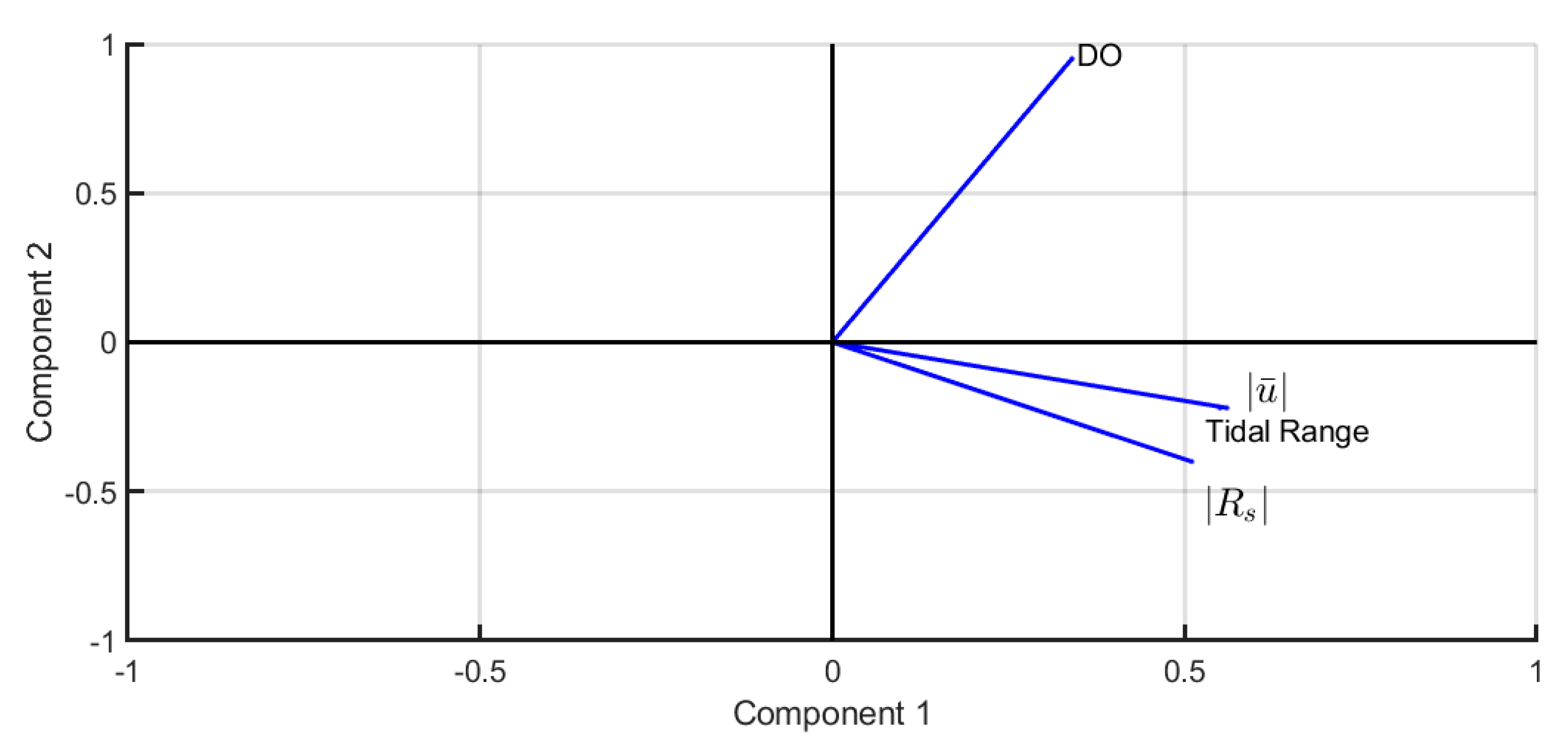
To complement the univariate statistical analysis linking water quality and hydrodynamics, the multivariate method of principal component analysis (PCA) explores relationships between current speed, tidal range, dissolved oxygen, and Reynolds shear stress. For this analysis, all variables are averaged over half a tidal cycle to match the sampling frequency of tidal range. All observations within each time series are scaled by the variance of the respective time series.
Principal components one and two explain 74% and 19% of the variation in the data, respectively (Figure 7). Component one loadings are as follows: dissolved oxygen (0.34), tidal range (0.55), Reynolds shear stress magnitude (0.51), and current speed (0.56). The large loading of DO concentration, tidal range, current speed, and Reynolds shear stress magnitude onto the same component indicates that they vary together. All loadings being positive suggests a direct relationship between them (i.e., as tidal range, Reynolds shear stress magnitude and current speed increase, dissolved oxygen increases as well). Because this analysis uses data sampled each half tidal cycle, these relationships mostly indicate net effects over multiple tidal cycles rather than within a cycle. The PCA supports our univariate statistical analysis results, which demonstrate that dissolved oxygen concentration increases over a tidal cycle when there is increased flushing and mixing promoted by an increased tidal range.
5. Conclusions
Larger tidal range in a tidal creek like Singleton Swash yields larger mean DO concentrations within the water column. Flood tides occur over shorter duration with stronger currents than ebb tides. Stronger tidal currents during flood tide generate larger Reynolds shear stress and greater mixing within the system. Flood tides import and mix oxygenated waters from the ocean throughout the system. Conversely, ebb tides, which transport oxygenated waters out of the creek and bring water with lower DO concentrations from the surrounding marsh closer to the channel mouth, are associated with periods of lower dissolved oxygen concentration. Larger tidal ranges cause stronger flood currents that transport higher volumes of oxygenated water into the creek and cause more mixing of DO throughout the system. This process overcomes the transport of water with lower DO concentrations from upstream on ebb tide resulting in a mean increase in DO over an entire tidal cycle. Consistent with these observations, smaller tidal ranges generate less transport into the creek coupled with less mixing, causing more retention of water (i.e., less exchange of waters). The lack of mixing and low transport of water from the ocean may also lead to heating of creek waters. These effects facilitate biological factors to potentially become more significant and lower the mean DO concentration within the system, possibly due to promoting net heterotrophic conditions.
Periodic maintenance of beach-face creek channel may be required to facilitate larger tidal ranges within the creek leading to an increase in the inventory of DO within the system. Hoffnagle [5] indicated that beach-face elevation exerts a primary control on the tidal range observed within Singleton Swash. The results of this study, connecting increased tidal ranges to hydrodynamic parameters and increases in DO, coupled with those from Hoffnagle [5], imply that maintaining lower beach-face elevation within the creek channel leads to larger tidal ranges, which generate greater mean DO concentrations and therefore promote a healthier ecosystem. To further aid in promoting healthy tidal creek ecosystems, future studies should examine the asymmetry of the tidal cycle and its relationship to beach-face morphology over a longer study period, as well as work toward development of a coupled geomorphic-hydrodynamic-biogeochemical model for deterministic prediction of the dynamics studied here.
Author Contributions
E.E.H. and D.M.P. conceived and designed the study. Field observations were performed by D.M.P. with contributions from D.B.F. and E.E.H. Data analysis was performed by D.M.P. under the supervision of E.E.H. and R.N.P. The first draft of the manuscript was written by D.M.P. and edited by all authors.
Funding
This research was funded in part by Horry County, South Carolina.
Acknowledgments
The authors would also like to thank Mathew J. Stanek, Ian J. Matsko, Christina Boraski, and Gina Guarriello for their aid in the field component of the study.
Conflicts of Interest
The authors declare no conflict of interest.
References
- Morris, J.T.; Sundareshwar, P.V.; Nietch, C.T.; Kjerfve, B.; Cahoon, D.R. Sea Level of Coastal Wetlands to Ristng Responses. Ecology 1992, 83, 2869–2877. [Google Scholar] [CrossRef]
- Kirwan, M.L.; Megonigal, J.P. Tidal wetland stability in the face of human impacts and sea-level rise. Nature 2013, 504, 53–60. [Google Scholar] [CrossRef] [PubMed]
- Brinson, M.M. Strategies for assessing the cumulative effects of wetland alteration on water quality. Environ. Manag. 1988, 12, 655–662. [Google Scholar] [CrossRef]
- Saiz-Salinas, J.I.; Gonzalez-Oreja, J.A. Stress in estuarine communities: Lessons from the highly-impacted Bilbao Estuary (Spain). J. Aquat. Ecosyst. Stress Recover. 2000, 7, 43–55. [Google Scholar] [CrossRef]
- Hoffnagle, B.L. Linking Water Quality and Beach Morphodynamics in a Heavily Impacted Tidal Creek in Myrtle Beach, South Carolina. Master’s Thesis, Coastal Carolina University, Conway, SC, USA, 2015. [Google Scholar]
- Voulgaris, G.; Meyers, S.T. Temporal variability of hydrodynamics, sediment concentration and sediment settling velocity in a tidal creek. Cont. Shelf Res. 2004, 24, 1659–1683. [Google Scholar] [CrossRef]
- Trowbridge, J.H. On a Technique for Measurement of Turbulent Shear Stress in the Presence of Surface Waves. J. Atmos. Ocean. Technol. 1998, 15, 290–298. [Google Scholar] [CrossRef]
- Trowbridge, J.H.; Geyer, W.R.; Bowen, M.M.; Williams, A.J. Near-Bottom Turbulence Measurements in a Partially Mixed Estuary: Turbulent Energy Balance, Velocity Structure, and Along-Channel Momentum Balance. J. Phys. Oceanogr. 1999, 29, 3056–3072. [Google Scholar] [CrossRef]
- Feddersen, F.; Trowbridge, J.H.; Williams, A.J. Vertical Structure of Dissipation in the Nearshore. J. Phys. Oceanogr. 2007, 37, 1764–1777. [Google Scholar] [CrossRef]
- Thorpe, S. The Turbulent Ocean; Cambridge University Press: Cambridge, UK, 2005. [Google Scholar]
- Elgar, S.; Raubenheimer, B.; Guza, R.T. Quality control of acoustic Doppler velocimeter data in the surfzone. Meas. Sci. Technol. 2005, 16, 1889. [Google Scholar] [CrossRef]
- Barnhardt, W.A. (Ed.) Coastal Change Along the Shore of Northeastern South Carolina—The South Carolina Coastal Erosion Study; U.S. Geological Survey Circular 1339: Reston, VA, USA, 2009.
- Pastore, D.M. Hydrodynamic Drivers of Dissolved Oxygen Variability Within a Highly Developed Tidal Creek. Master’s Thesis, Coastal Carolina University, Conway, SC, USA, 2018. [Google Scholar]
- Fagherazzi, S.; Hannion, M.; Odorico, P.D. Geomorphic structure of tidal hydrodynamics in salt marsh creeks. Water Resour. Manag. 2008, 44. [Google Scholar] [CrossRef]
- Svendsen, I.A. Introduction to Nearshore Hydrodynamics; World Scientific Publishing Co. Pte. Ltd.: Hackensaack, NJ, USA, 2006. [Google Scholar]
- Dean, R.G.; Dalrymple, R.A. Water Wave Mechanics for Engineers and Scientists; Liu, P., Ed.; World Scientific Publishing Co. Pte. Ltd.: Hackensaack, NJ, USA, 1991. [Google Scholar]
- Troup, M.L.; Fribance, D.B.; Libes, S.M.; Gurka, R.; Hackett, E.E. Physical Conditions of Coastal Hypoxia in the Open Embayment of Long Bay, South Carolina: 2006–2014. Estuaries Coasts 2017, 40, 1576–1591. [Google Scholar] [CrossRef]
- Aubrey, D.G.; Speer, P.E. A study of non-linear tidal propagation in shallow inlet/estuarine systems Part I: Observations. Estuar. Coast. Shelf Sci. 1985, 21, 185–205. [Google Scholar] [CrossRef]
- O’Laughlin, C.; Van Proosdij, D.; Milligan, T.G. Flocculation and sediment deposition in a hypertidal creek. Cont. Shelf Res. 2014, 82, 72–84. [Google Scholar] [CrossRef]
- Dronkers, J. Tidal asymmetry and estuarine morphology. Neth. J. Sea Res. 1986, 20, 117–131. [Google Scholar] [CrossRef]
- Blanton, J.O.; Lin, G.; Elston, S.A. Tidal current asymmetry in shallow estuaries and tidal creeks. Cont. Shelf Res. 2002, 22, 1731–1743. [Google Scholar] [CrossRef]
- Cimbala, J.M.; Çengel, Y.A. Essentials of Fluid Mechanics: Fundamentals and Applications; McGraw-Hill Higher Education: New York, NY, USA, 2008. [Google Scholar]
- Marusic, I.; McKeon, B.J.; Monkewitz, P.A.; Nagib, H.M.; Smits, A.J.; Sreenivasan, K.R. Wall-bounded turbulent flows at high Reynolds numbers: Recent advances and key issues. Phys. Fluids 2010, 22, 065103. [Google Scholar] [CrossRef]
Figure 1.
(A) satellite image of the southeastern United States with emphasis on the Long Bay area, located between North Carolina (NC) and South Carolina (SC). The location of the study area is approximated by the red “x” and the state border is defined by the light blue line; (B) aerial photo of Singleton Swash tidal creek showing the most dynamic area of the swash between the waterline and beach dune as well as the surrounding watershed. Measurement locations for this study are also labeled as Site A, Site B, and Site C.

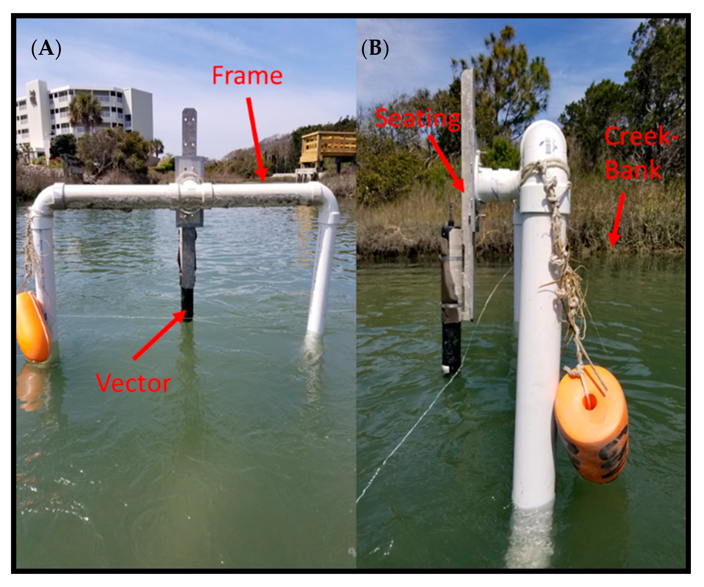
Figure 2.
(A) along-channel and (B) cross-channel view of the Vector, seating, and frame at low tide. The Vector is approximately centered across the channel width.
Figure 2.
(A) along-channel and (B) cross-channel view of the Vector, seating, and frame at low tide. The Vector is approximately centered across the channel width.

Figure 3.
(A) sample time series of all three velocity components on 6 May 2018 beginning at 16:00, where the along-channel velocity (u) is blue, the across-channel velocity (v) is red, and the vertical velocity (w) is yellow; (B) power spectral density of along-channel velocity in (A), exhibiting a peak at a frequency within the approximate timescales for wind waves (~1 Hz). Such a record would be excluded from calculation of Reynolds shear stresses (see Section 3.3).

Figure 4.
Sample time series of percent (%) saturation of dissolved oxygen at Site B over a period of 15 days. Daylight hours (x) begin at 6:00 a.m. and end at 8:00 p.m. and non-daylight hours (x) range from 8:00 p.m. to 6:00 a.m. Regions of light blue denote times during spring tide while the grey denotes periods of neap tide.

Figure 5.
(A) time series of along-channel current velocity () measured by the ADV during the May, 2018 deployment; (B) power spectral density (PSD) of current velocity () shown in (A). The highest spectral peak occurs at a period of 12.5 h.
Figure 5.
(A) time series of along-channel current velocity () measured by the ADV during the May, 2018 deployment; (B) power spectral density (PSD) of current velocity () shown in (A). The highest spectral peak occurs at a period of 12.5 h.

Figure 6.
Time series of Reynold shear stress () calculated from velocity measurements recorded by the ADV over the May deployment.
Figure 6.
Time series of Reynold shear stress () calculated from velocity measurements recorded by the ADV over the May deployment.

Figure 7.
Bi-plot of principal components one and two resulting from a PCA on variables: current speed (), Reynolds shear stress magnitude (), tidal range, and dissolved oxygen (DO). Blue lines represent loading of each variable onto each principle component. Principle component one and two represent 74% and 19% of the dataset variance, respectively.


Table 1.
Time series used in Equation (4) for both correlation variables (p, q), sampling period (T), location of the measurement corresponding to each variable, and the instrument used to perform the measurement.
Table 1.
Time series used in Equation (4) for both correlation variables (p, q), sampling period (T), location of the measurement corresponding to each variable, and the instrument used to perform the measurement.
| p | q | T (Days) | Location of Measurements (p/q) | Instruments (p/q) |
|---|---|---|---|---|
| Tidal Range (m) | Tidal Range (m) | 131 | Site A/Site C | HOBO water level logger/HOBO water level logger |
| Tidal Range (m) | Max Flood Current (m/s) | 31 | Site A/Site B | HOBO water level logger/Vector |
| Tidal Range (m) | Max Ebb Current (m/s) | 31 | Site A/Site B | HOBO water level logger/Vector |
| Tidal Range (m) | Flood Discharge (m3) | 31 | Site A/Site B | HOBO water level logger/Vector |
| Tidal Range (m) | Ebb Discharge (m3) | 31 | Site A/Site B | HOBO water level logger/Vector |
| Reynolds Shear Stress (N/m2) | (m/s) | 31 | Site B/Site B | Vector/Vector |
| Dissolved Oxygen (% saturation) | Reynolds Shear Stress (N/m2) | 31 | Site B/Site B | HOBO DO logger/Vector |
| Dissolved Oxygen (% saturation) | Flood Discharge (m3) | 31 | Site B/Site B | HOBO DO logger/Vector |
| Dissolved Oxygen (% saturation) | Ebb Discharge (m3) | 31 | Site B/Site B | HOBO DO logger/Vector |
| Dissolved Oxygen (% saturation) | (m/s) | 31 | Site B/Site B | HOBO DO logger/Vector |
| Dissolved Oxygen (% saturation) | Tidal Range (m) | 271 | Site A/Site A | HOBO DO logger/HOBO water level logger |
| Dissolved Oxygen (% saturation) | Wind Speed (m/s) | 31 | Site B/Apache pier | HOBO DO logger/Met station |
Table 2.
Correlated parameters (p and q; Equation (4)) with the corresponding maximum correlation coefficients, upper and lower 95% confidence intervals (lower: CIL; upper: CIH), lag time, correlation time series resolution (CR), and correlation time interval (CI).
Table 2.
Correlated parameters (p and q; Equation (4)) with the corresponding maximum correlation coefficients, upper and lower 95% confidence intervals (lower: CIL; upper: CIH), lag time, correlation time series resolution (CR), and correlation time interval (CI).
| p | q | R | 95% ClL | 95% CIH | Lag (Hours) | CR (Hours) | CI (Days) |
|---|---|---|---|---|---|---|---|
| Tidal Range (m) | Flood Q (m3) | 0.754 | 0.62 | 0.89 | 0 | 12.00 | 30.0 |
| Tidal Range (m) | Ebb Q (m3) | 0.977 | 0.96 | 0.99 | 0 | 12.00 | 30.0 |
| Tidal Range Site A (m) | Tidal Range Site C (m) | 0.981 | 0.98 | 0.98 | 0 | 12.00 | 14.0 |
| Tidal Range (m) | Max Flood Current (m/s) | 0.927 | 0.92 | 0.93 | 0 | 1.00 | 1.0 |
| Tidal Range (m) | Max Ebb Current (m/s) | 0.842 | 0.83 | 0.85 | 0 | 1.00 | 1.0 |
| Reynolds Shear Stress (N/m2) | (m/s) | 0.434 | 0.40 | 0.46 | 0 | 0.25 | 0.5 |
| Dissolved Oxygen (% saturation) | (m/s) | −0.511 | −0.55 | −0.47 | 1.75 | 0.25 | 2.0 |
| Dissolved Oxygen (% saturation) | Flood Q (m3) | 0.608 | 0.32 | 0.89 | 0 | 12.00 | 10.0 |
| Dissolved Oxygen (% saturation) | Ebb Q (m3) | −0.541 | −0.74 | −0.34 | 0 | 12.00 | 10.0 |
| Dissolved Oxygen (% saturation) | Wind Speed (m/s) | 0.274 | 0.19 | 0.36 | 1.00 | 0.08 | 14.0 |
| Dissolved Oxygen (% saturation) | Reynolds Shear Stress (N/m2) | 0.276 | 0.24 | 0.31 | 0 | 0.25 | 0.5 |
| Dissolved Oxygen (% saturation) | Tidal Range (m) | 0.277 | 0.03 | 0.53 | 36 | 12.00 | 14.0 |
© 2019 by the authors. Licensee MDPI, Basel, Switzerland. This article is an open access article distributed under the terms and conditions of the Creative Commons Attribution (CC BY) license (http://creativecommons.org/licenses/by/4.0/).
Share and Cite
MDPI and ACS Style
Pastore, D.M.; Peterson, R.N.; Fribance, D.B.; Viso, R.; Hackett, E.E. Hydrodynamic Drivers of Dissolved Oxygen Variability within a Tidal Creek in Myrtle Beach, South Carolina. Water 2019, 11, 1723. https://doi.org/10.3390/w11081723
AMA Style
Pastore DM, Peterson RN, Fribance DB, Viso R, Hackett EE. Hydrodynamic Drivers of Dissolved Oxygen Variability within a Tidal Creek in Myrtle Beach, South Carolina. Water. 2019; 11(8):1723. https://doi.org/10.3390/w11081723
Chicago/Turabian StylePastore, Douglas M., Richard N. Peterson, Diane B. Fribance, Richard Viso, and Erin E. Hackett. 2019. "Hydrodynamic Drivers of Dissolved Oxygen Variability within a Tidal Creek in Myrtle Beach, South Carolina" Water 11, no. 8: 1723. https://doi.org/10.3390/w11081723
Note that from the first issue of 2016, this journal uses article numbers instead of page numbers. See further details here.