Regional Flood Frequency Analysis for a Poorly Gauged Basin Using the Simulated Flood Data and L-Moment Method

1
Department of Civil Engineering, Kyung Hee University, Yongin 17104, Korea
2
Department of Land, Water and Environment Research, Korea Institute of Civil Engineering and Building Technology, Goyang 10223, Korea
*
Author to whom correspondence should be addressed.
Water 2019, 11(8), 1717; https://doi.org/10.3390/w11081717
Submission received: 31 July 2019
/
Revised: 16 August 2019
/
Accepted: 16 August 2019
/
Published: 18 August 2019
(This article belongs to the Section Hydrology)
Abstract
:The design of hydraulic structures and the assessment of flood control measures require the estimation of flood quantiles. Since observed flood data are rarely available at the specific location, flood estimation in un-gauged or poorly gauged basins is a common problem in engineering hydrology. We investigated the flood estimation method in a poorly gauged basin. The flood estimation method applied the combination of rainfall-runoff model simulation and regional flood frequency analysis (RFFA). The L-moment based index flood method was performed using the annual maximum flood (AMF) data simulated by the rainfall-runoff model. The regional flood frequency distribution with 90% error bounds was derived in the Chungju dam basin of Korea, which has a drainage area of 6648 km2. The flood quantile estimates based on the simulated AMF data were consistent with the flood quantile estimates based on the observed AMF data. The widths of error bounds of regional flood frequency distribution increased sharply as the return period increased. The results suggest that the flood estimation approach applied in this study has the potential to estimate flood quantiles when the hourly rainfall measurements during major storms are widely available and the observed flood data are limited.
1. Introduction
Flood estimates are needed to design hydraulic structures and assess flood control measures. Since flood data in the investigated location are rarely available, reliable estimation of flood quantiles in un-gauged or poorly gauged basins is a common problem in engineering hydrology. In the past, various regional flood frequency analysis (RFFA) methods have been applied to estimate the flood quantiles in ungauged or poorly gauged basins [1,2]. The RFFA can be performed by pooling the flood discharge data observed at different sites within a region. However, it is very difficult to perform the RFFA in Korea because of limited regional flood discharge data. In practice, the flood quantiles in Korea are generally estimated using the rainfall-based design event approach. The design event approach is based on the transformation of design rainfall into design flood [3,4].
The joint probability approach has been proposed to resolve the limitations of the design event approach. The joint probability approach considers probability-distributed inputs and model parameters using a Monte Carlo simulation approach [4,5]. Continuous simulation approaches have become more popular as a complement to the RFFA. The continuous simulation approach applies the continuous model with long rainfall inputs to derive the flood frequency distribution [6,7,8]. These methods might have computational constraints for applications in engineering practice.
In this study, we explore the alternative flood estimation method, which applies the combination of event rainfall-runoff model simulation and the RFFA. First, the rainfall-runoff model simulates the regional flood data for major storm events. Subsequently, the L-moment based index flood method is performed using the simulated annual maximum flood (AMF) sampled at many sites within a homogeneous region. The flood estimation method developed in this study is motivated by the following consideration. Rainfall data for major storms are widely available at the study basin. The L-moment method provides less bias in flood estimation and is universally applied in the literature [9,10,11,12,13,14,15,16].
Use of the simulated flood data in the RFFA was previously proposed by Kim et al. [17]. They applied the RFFA to AMF data generated from the storage function runoff model. They called their approach the spatial data extension method. Since the RFFA that employs the spatial data extension method is based on the simulated AMF, it is important to assess the applicability of the method in the RFFA. In this study, we aim to test the spatial data extension method using a rainfall-runoff model and modeling strategy which are different from the previous study [17]. The proposed rainfall-runoff modeling strategy allowed us to generate the AMF data in a poorly gauged basin. In the present context, the poorly gauged basin is the basin which has long-term flood data at one or two hydrometric stations such that it is infeasible to apply RFFA using the observed AMF. The simulated AMF data were used to derive a regional growth curve and index flood in the study basin. The uncertainty of the regional growth curve was also estimated using the Monte Carlo simulation approach suggested by Hosking and Wallis [9]. The estimated flood quantiles were evaluated using the AMF data observed at the outlet and one interior location in the study basin. Our results were compared to those of the previous study [17] to assess the applicability of the developed flood estimation method.
2. Materials and Methods
2.1. Study Region and Data
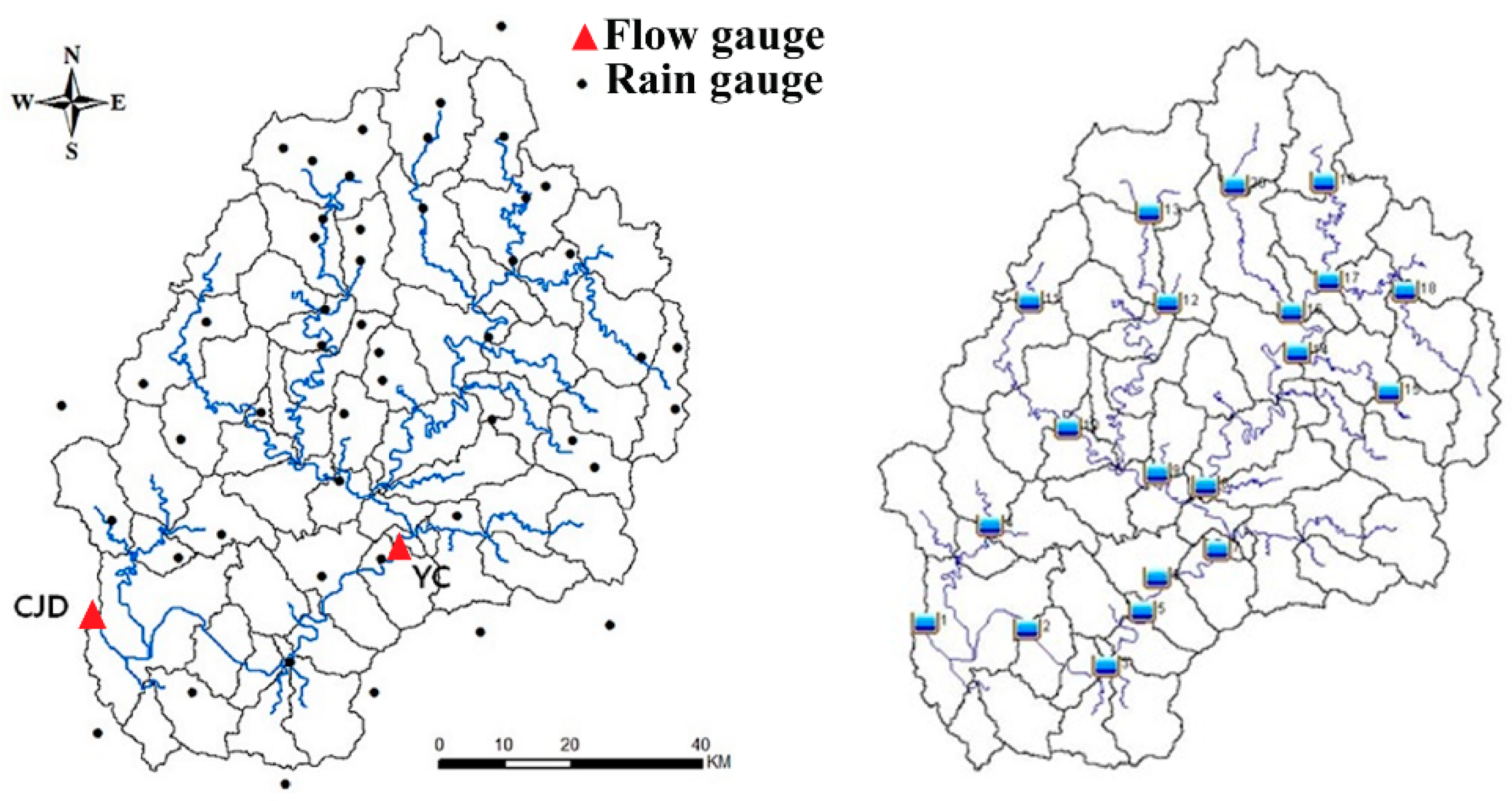
In this study, we investigated in the Chungju dam basin, which is located on the Namhan river in Korea. The drainage area of the basin is 6648 km2, and the Chungju dam (CJD) is located at the outlet of the basin (Figure 1). The average annual precipitation is 1330 mm, and 70% of the rain falls in the monsoon season from June to September [18]. The main land use type of the basin is forests, which occupy 82% and the agricultural area covers 13% of the basin.
Figure 1 shows the rainfall and discharge stations used in this study. Major storm events for each year were selected from 1987 to 2010 (Table S1 in Supplementary Materials). These storm events would produce the maximum peak discharge in a given year. For some years, multiple storm events are considered to sample the maximum peak discharge at various sites because the maximum peak discharge at various sites depends on the spatial and temporal variability of rainfall characteristics. The flood data were collected at two locations: The dam inflow data at the CJD and the water level data measured at the Yeongchun (YC) station were converted into discharge using rating curve. The studied basin is considered a poorly gauged basin because long-term flood data are available only at two hydrometric stations. These hydrological data have been managed by K-Water (http://www.kwater.or.kr) and WAMIS (http://www.wamis.go.kr). The other data used for the analysis are the DEM, with 30 m resolution, a 1:25,000 land cover map constructed by Ministry of Environment, and a 1:25,000 soil map constructed by National Institute of Agricultural Sciences. The hydrologic soil groups classified for Korean soils are also available from the National Institute of Agricultural Sciences.
2.2. Generation of Regional Flood Data Using Rainfall-Runoff Model
The simulation of regional flood data in this study is based on HEC-HMS [19]. The HEC-HMS provides various components and models for rainfall-runoff modeling. The event simulation of the rainfall-runoff relation requires models for rainfall loss, excess rainfall transformation, baseflow, and channel flow routing. The loss of rainfall is based on the SCS curve number method. The transformation of excess rainfall into runoff is calculated using the SCS and Clark unit hydrograph methods. The reasons for using these unit hydrograph methods are twofold: (1) the number of parameters in the unit hydrograph methods is small and (2) the parameters can be identified using the empirical formula developed for the Chungju dam basin. A simple model with a reduced number of parameters was suggested to simulate flood formation process to reduce the uncertainty of model predictions [20,21]. The exponential recession model was applied for modeling baseflow components. The Muskingum–Cunge model was used for channel flow routing. The Muskingum–Cunge model is a physically based model and can be used for ungauged watersheds. The HEC-HMS manual provides detailed descriptions for the equations of rainfall-runoff components.
The first step in setting up HEC-HMS is to delineate sub-watersheds and stream networks. The entire Chungju dam basin is divided into 57 sub-watersheds based on map of the standard watershed (Figure 1). The standard watersheds in Korea are defined for the effective identification of watersheds and the management of water resources (http://www.wamis.go.kr). The average areal rainfall for each sub-watershed is defined by the Thiessen polygon method.
The parameters and conditions for each watershed and channel reach should be identified to simulate the response of rainfall-runoff relations. For a gauged watershed, a calibration can be performed to identify the model parameters using the observed flow data. However, it is difficult to identify the model parameters in an ungauged or poorly gauged watershed. Predicting ungauged basins has been a great challenge for hydrology community [22,23].
The parameters related to SCS curve number model are the initial abstraction ratio () and curve number (). The empirical relationship between initial abstraction () and potential maximum retention () is given as
The relationship between and is given as
The initial abstraction ratio in the original SCS curve number equation is defined as = 0.2. However, many studies suggested a different value of 0.05 [24,25]. We applied two different initial abstraction ratios of = 0.2 and = 0.05. The use of = 0.05 requires a new set of values [25]. The values for = 0.05 can be obtained from values for = 0.2 as
For the ungauged watershed, the curve number can be estimated from the table of USDA-NRCS [26] based on land use/cover and soil information. The curve number might vary from event to event, and the variation in the results from differences in rainfall intensity and duration, total rainfall, soil moisture conditions, cover density, stage of growth, and temperature [26]. The three classes of antecedent runoff conditions (ARC) are defined in USDA-NRCS [26] to reflect the variability in : ARC II for average conditions, ARC I for dry conditions, ARC III for wet conditions.
The parameters needed for Clark and SCS unit hydrograph models are the time of concentration (), storage coefficient () and lag time (). Lee et al. [27] developed a regionalized empirical formula for and in the Chungju dam basin. The empirical formulas are expressed as a function of channel length () and channel slope ():
The USDA-NRCS [26] suggests the relationship between and :
These empirical formulas are applied to estimate the parameters , and for each sub-watershed.
The Muskingum–Cunge model for channel flow routing requires a description of channel cross section, reach length, roughness coefficient, and energy slope. The trapezoidal channel configuration was assumed to be a representative cross section. The energy slope was estimated by the channel bed slope. The various field investigation reports in WAMIS were used to estimate the principal dimension of channel section, reach length, and Manning roughness coefficients. A total of 42 reaches were defined for setting up the Muskingum–Cunge model in the Chungju dam basin. One representative cross section per reach was defined in setting up the Muskingum–Cunge model.
The exponential recession model includes a specification for the initial baseflow and an exponential decay constant. The initial baseflow is assumed to be equal to an initial discharge at the start of the storm event. The specific discharges (discharge per unit area) for each storm event were estimated using initial discharges observed at the CJD and YC stations. The average specific discharge was estimated to be 0.04 m3/s/km2 in the Chungju dam basin. The initial baseflow for each sub-watershed can be specified by multiplying the specific discharge by the area of a sub-watershed. The exponential decay constant suggested by Pilgrim and Cordery [28] was used in the simulation.
A number of simulations for each storm event were carried out using a combination of two unit hydrograph methods (Clark and SCS), two values (0.2 and 0.05), and two ARC levels (II and III). The selections of these conditions and methods were based on conditioning the observed peak discharge data of each storm event at the CJD and YC stations. After the regional flood data were simulated for each storm event, the simulated AMF data at various sites were extracted by selecting the largest peak discharge in a given year.
2.3. Regional Flood Frequency Analysis
2.3.1. Index Flood Method
The index flood method originally proposed by Dalrymple [29] is based on the main hypothesis that the frequency distributions of sites within a homogeneous region are identical apart from a site-specific scaling factor (index flood). The quantile function at a site , is estimated by the product of the index flood () and regional growth curve as
In the equation, implies the non-exceedance probability. The regional growth curve is the dimensionless frequency distribution common to all sites within a homogeneous region. The index flood is usually estimated as the mean of the AMF data at a site . The other location estimator (such as a median) can be used as the index flood [14]. Bocchiola et al. [30] reviewed the various methods for estimating index flood at gauged and ungauged watersheds.
2.3.2. L-moment
The L-moment has theoretical advantages over the conventional moments. In contrast to the conventional moments, the L-moment is reliably applied for the regional frequency analysis [9]. The L-moment can characterize a wide range of distributions. The location, scale, and shape estimators of the L-moment are unbiased irrespective of the probability distribution. The L-moments are more robust to the presence of outliers in the data and are related to the probability weighted moment (PWM). Greenwood et al. [31] introduced the PWM of a random variable and the L-moment is defined by the linear combinations of PWM. Using the location measure () and scale measure (), Hosking and Wallis [9] defined the L-moment ratios as:
- L-CV: τ = λ2/λ1
- L-skewness: τ3 = λ3/λ2
- L-kurtosis: τ4 = λ4/λ2
For a distribution which takes only positive values, the range of L-CV is 0 < 1. The ranges of L-skewness and L-kurtosis are given as −1 < < 1 and −1 < < 1.
2.3.3. Discordancy and Heterogeneity Measure
The statistical tests for AMF data need to be performed to check the adequacy of data used for the RFFA. The randomness test is based on the randtests package in R software [32]. The Kendall package (https://www.rdocumentation.org/packages/Kendall/versions/2.2) based on the method of Mann [33] was applied for the trend test. The outlier test was performed by the Bulletin 17B method [34] and the G-B method [35]. These tests indicated that the simulated AMF data satisfied all assumptions needed for the RFFA.
A discordancy measure can be used to check that the data are valid for the regional frequency analysis. It allows one to detect sites that are discordant with the group as a whole. Hosking and Wallis [9] defined the discordancy measure for a site as
where is the number of sites, = is the vector containing the L-moment ratios, is the un-weighted group average of , and is the sample covariance matrix of sums of squares and cross-products. The site is considered to be discordant with the group when is greater than the critical value. The critical values depend on the number of sites in the region. When the number of sites in the region exceeds 15, the critical value is three [9].
A test of regional homogeneity is required for the regional frequency analysis to assess whether a proposed region might be regarded as a homogeneous region. The heterogeneity measure was proposed to estimate the degree of heterogeneity in a group of sites [36]. The heterogeneity measure compares the between-site dispersion of the sample L-moment ratios for the region under consideration with that of the simulated L-moment ratios for a homogeneous region. A simple measure of the between-site dispersion of the L-moment ratios is the weighted standard deviation of the L-moment ratios.
The heterogeneity statistic () can be calculated as
where is the weighted standard deviation of the observed L-CV, and and are the mean and standard deviation of values of calculated for each simulated homogeneous region. The Monte Carlo simulation was used to generate realizations of a homogeneous region whose frequency distribution was the kappa distribution with four parameters. The proposed region is considered to be heterogeneous when is sufficiently large. Hosking and Wallis [9] suggest that the region under consideration is “acceptably homogeneous” if < 1, “possibly heterogeneous” if 1 < 2, and “definitely heterogeneous” if ≥ 2.
2.3.4. Selection and Estimation of Regional Growth Curve
There are different methods for selecting an appropriate regional frequency distribution that describes the features of the sample data. The L-moment ratio diagram plots L-skewness versus L-kurtosis. This plot can be used for a visual comparison of L-moment ratios between sample data and candidate distributions. The selection of a frequency distribution based on the L-moment diagram is not quantitative and rather subjective. However, there are some quantitative measures proposed in the literature. The statistic proposed by Hosking and Wallis [9] is defined as
In this equation, indicates any candidate distribution. The three parameter distributions applied for the RFFA are the generalized logistic (GLO), generalized extreme value (GEV), generalized normal (GNO), Pearson type III (PE3), and generalized Pareto (GP). The L-kurtosis of the fitted distribution is indicated by , and is the regional average L-kurtosis weighted proportionally to the record length of sites. The bias of is indicated by , and is the standard deviation of . The calculation of and is based on the fitting of a kappa distribution and Monte Carlo simulation of kappa distributed regions. Further details of calculating and can be explained in Hosking and Wallis [9]. Any candidate distributions are considered to be adequate fits when ≤ 1.64.
Kroll and Vogel [37] proposed the average weighted orthogonal distance (AWOD). The AWOD measures the average weighted distance between sample L-moment ratios and theoretical L-moment ratios of a given frequency distribution. The AWOD is defined as
where is the orthogonal distance between the sample L-kurtosis at site and the theoretical L-kurtosis for a given distribution. A candidate distribution having the smallest AWOD value is considered as the best distribution.
Once the appropriate regional frequency distribution is identified, the form of the regional growth curve is known apart from the undetermined parameters. The regional L-moment algorithm is applied to estimate the undetermined parameters using L-moment ratios [9].
2.3.5. The Accuracy of the Estimated Regional Growth Curve
Results of statistical analysis might be uncertain, and some assessment of uncertainty should be performed. The Monte Carlo simulation approach was suggested by Hosking and Wallis [9] to estimate the accuracy of the estimated regional frequency distribution. The simulations should agree with the specific characteristics of the data from which the estimates are computed. Hence, the number of sites, record length at each site, and the regional average L-moments ratios of the simulated region are the same as those of the actual region. The simulated region might include heterogeneity and inter-site dependence of the data. The heterogeneity measure computed from the simulated region needs to be consistent with that computed from the actual region. The observed sample L-moment ratios cannot be used as the population L-moment ratios of the simulated region because this will result in a simulated region that has much more heterogeneity than the actual region [9]. Therefore, the variations in the L-moment ratios of the simulated region are usually set to be less than that of sample L-moment ratios of the actual region.
According to Hosking and Wallis [9], the overall accuracy measure for the estimated regional growth curve is given as
In this equation, implies the regional average relative RMSE of the estimated regional growth curve. The relative RMSE of the estimated regional growth curve at a site i averaged over all averaged over all simulations is given as
In this equation, indicates the estimated growth curve of a site at the mth repetition, and implies the true growth curve of a site . For a homogeneous region, the growth curves are the same at all sites such that and in Equation (12) can be replaced with and . Hosking and Wallis [9] defined 90% error bounds for the estimated growth curve as
In this relation, is some value below which 5% of the simulated values of lie, and is some value above which 5% of the simulated values of lie.
2.4. Performance Evaluation Measures
The coefficient efficiency (CE) and coefficient of persistence (CP) were used as the evaluation measure of the simulated results. Cheng et al. [38] suggested the use of these two measures for the evaluation of real-time flood forecasting model. The CE and CP are defined as
is the observed value at time t, is the average of the observed value, is the simulated value at time t. Since the average time of concentration for sub-watersheds of this study basin is about 4 h, the CP is estimated using k = 3 h. The CE and CP differ only in the denominator term. The CE and CP values range from −∞ to 1. The model performance is the best when CE and CP values become one.
3. Results
3.1. Assessment of the Simulated Flood Discharge
To understand the adequacy of the simulated flood discharge, the simulation performance was assessed at two locations. The assessment results for the simulated hydrographs were described in Table S2 of the Supplementary Materials. For some storm events, the CE and CP values are not given in Table S2 because some parts of the observed discharge hydrograph are not reliable. The computed CE values for the simulated hydrographs ranged from 0.62 to 0.98 while the computed CP values ranged from −5.41 to 0.74. The performance of the simulated hydrographs was satisfactory in terms of CE measure. But the simulation results for low and medium peak discharges exhibited poor performance with low CP values. The Supplementary Materials (Figures S1–S3) illustrate the comparison of the simulated and observed hourly hydrographs selected from storm events with high, medium and low peak discharges. The simulated and observed hydrographs were in good agreement for large flood events (Figure S1) while the medium and small flood events (Figures S2 and S3) showed less agreement between simulated and observed hydrographs.
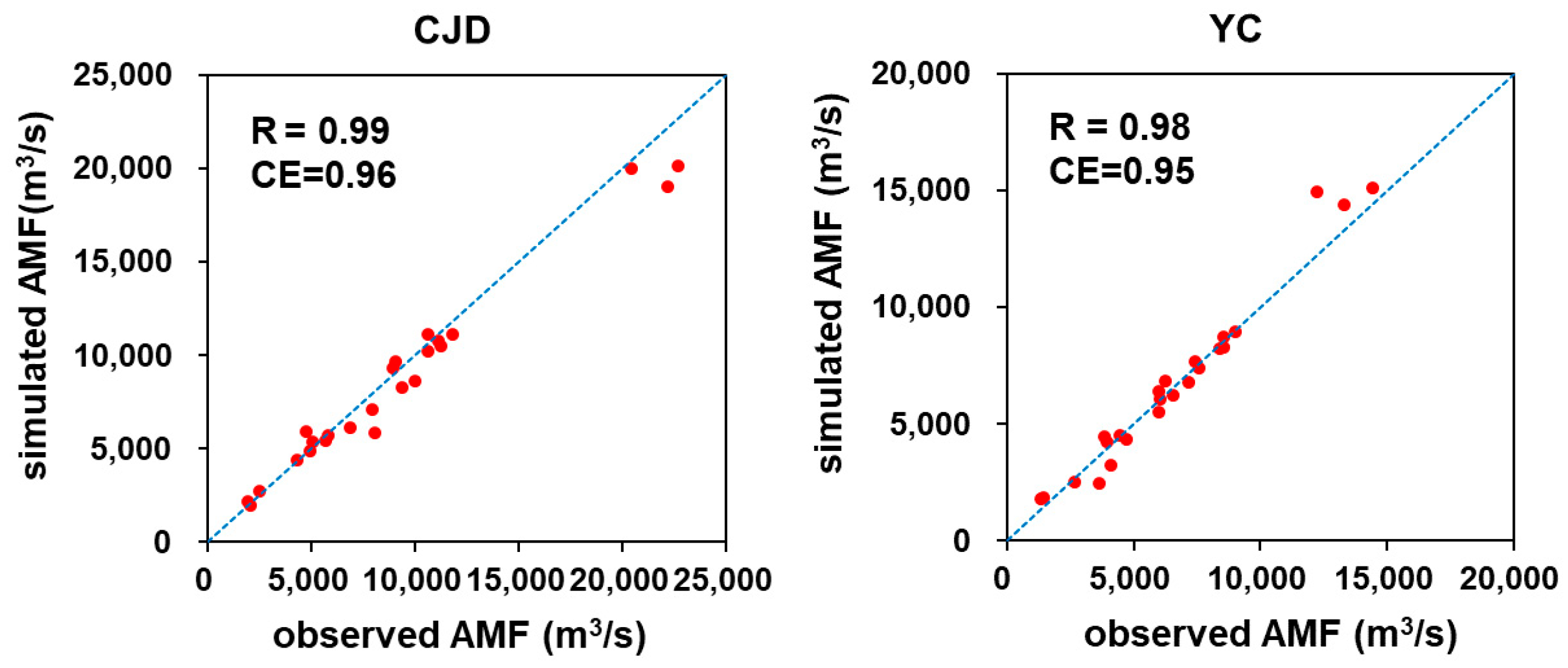
Figure 2 compares the observed AMF with the simulated AMF at CJD and YC locations. The simulated AMF shows good agreement with the observed AMF. The estimated coefficient of correlation exceeds 0.98 for both locations. The computed CE value was 0.96 for the CJD location and 0.95 for the YC location. It is noted that for very large flood events, there is a trade-off in simulation performance between CJD and YC since the AMF is underestimated in CJD and overestimated in YC. This indicates that there is a difficulty in identifying the spatial parameters and conditions for a semi-distributed rainfall-runoff model. Based on the assessment of the simulated flood responses at two locations, we hypothesize that the simulated flood responses are a reasonable approximation to the actual flood responses throughout the study basin.
3.2. Regional Flood Frequency Distribution and its Uncertainty
The flood quantiles at any sites within a homogeneous region can be estimated by Equation (6). The regional growth curve in Equation (6) was estimated using the RFFA based on the simulated AMF data at the 20 sites shown in Figure 1. The watershed area of the sites is very diverse and ranges from 109 km2 to 6648 km2. Hosking and Wallis [9] suggested that there is little gain in accuracy for RFFA using more than 20 sites.
Identification of the homogeneous region can be performed by applying the discordancy measure of Equation (7) and heterogeneity measure of Equation (8). The computed discordancy values for 20 sites ranged from 0.09 to 2.06. Since the computed discordancy values were less than the critical value of three, no sites were discordant with the group. The heterogeneity measure was estimated as = −0.59. The negative value of might be related to a positive correlation between AMF data at different sites. Therefore, the entire Chungju dam region was considered to be acceptably homogeneous because was less than one.
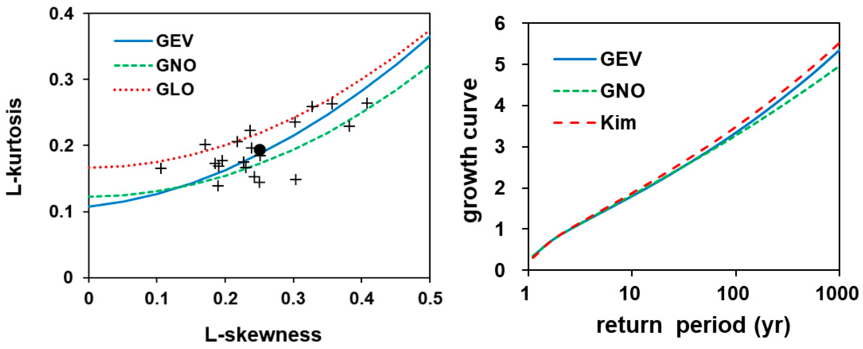
The goodness-of-fit measure was computed by Equation (9) to test whether the candidate distributions fit the AMF data closely. Table 1 shows statistics calculated for five candidate distributions. The values of three distributions (GLO, GEV, and GNO) are lower than the critical value of 1.64. For these distributions, Table 1 shows AWOD values calculated using Equation (10). It appears that the GEV distribution has the lowest and AWOD values. The L-moment ratio diagram is plotted in Figure 3 to compare the theoretical and sample L-moment ratios. The filled circle dot in the figure indicates the regional average of sample L-moment ratios.
Once the homogeneity of the region was tested and the proper regional frequency distribution was selected, the regional growth curve can be estimated using a regional L-moment algorithm explained in Section 2.3. The estimated growth curves are shown in the Figure 3. The growth curves for GEV and GNO distributions were considered and compared with the result of the previous study [17]. The estimated growth curves between GEV and GNO distributions were very similar for the return period smaller than 100 years.
The Monte Carlo simulation approach explained in Section 2.3.5 was applied to assess the uncertainty of the estimated growth curve. In the simulations, the following statistics between the simulated region and the actual region were set to be the same: The record length at each site, the regional average L-moments ratios and the average inter-site correlation. The range of L-CV and L-skewness of a simulated region was set to 0.13, which is smaller than the range of sample L-moment ratios. The average heterogeneity values computed from 500 simulated regions were = 0.23 for the GEV distribution and = 0.39 for the GNO distribution. Since these values were slightly higher than those of actual region, a little more heterogeneity was allowed in the simulation.
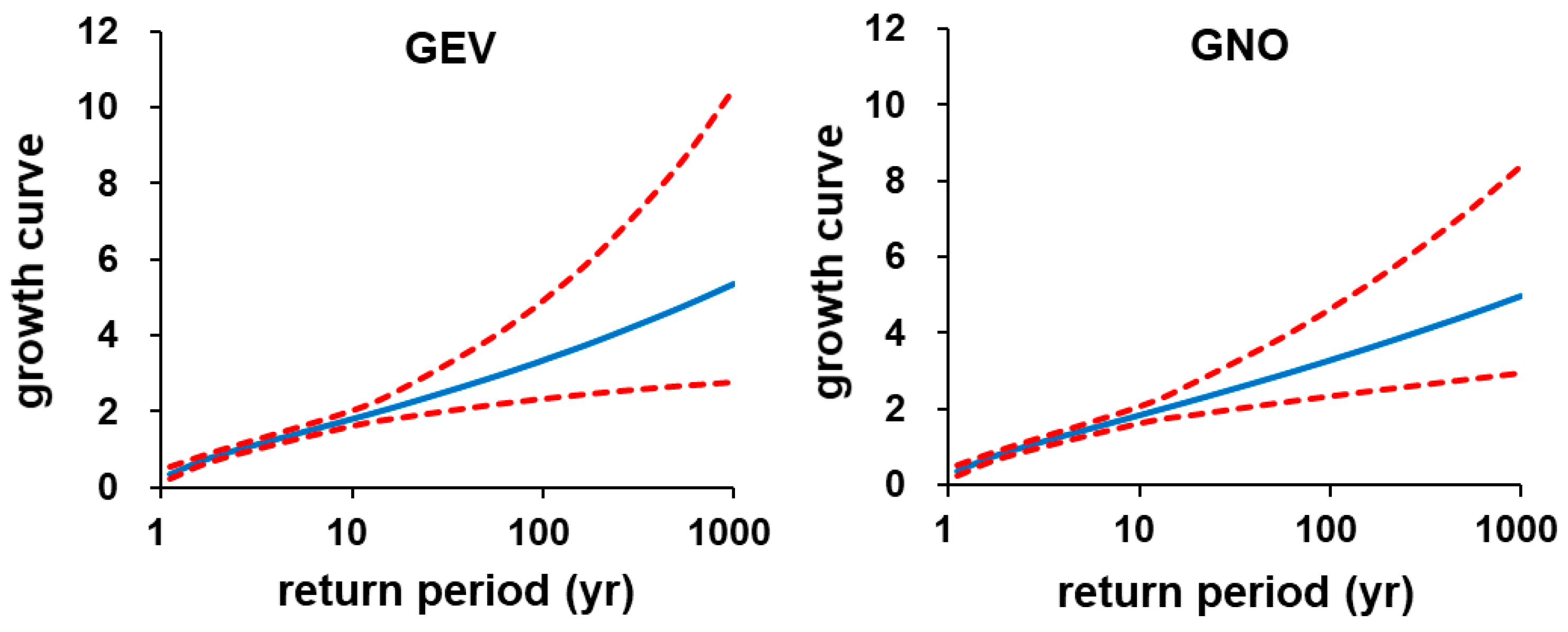
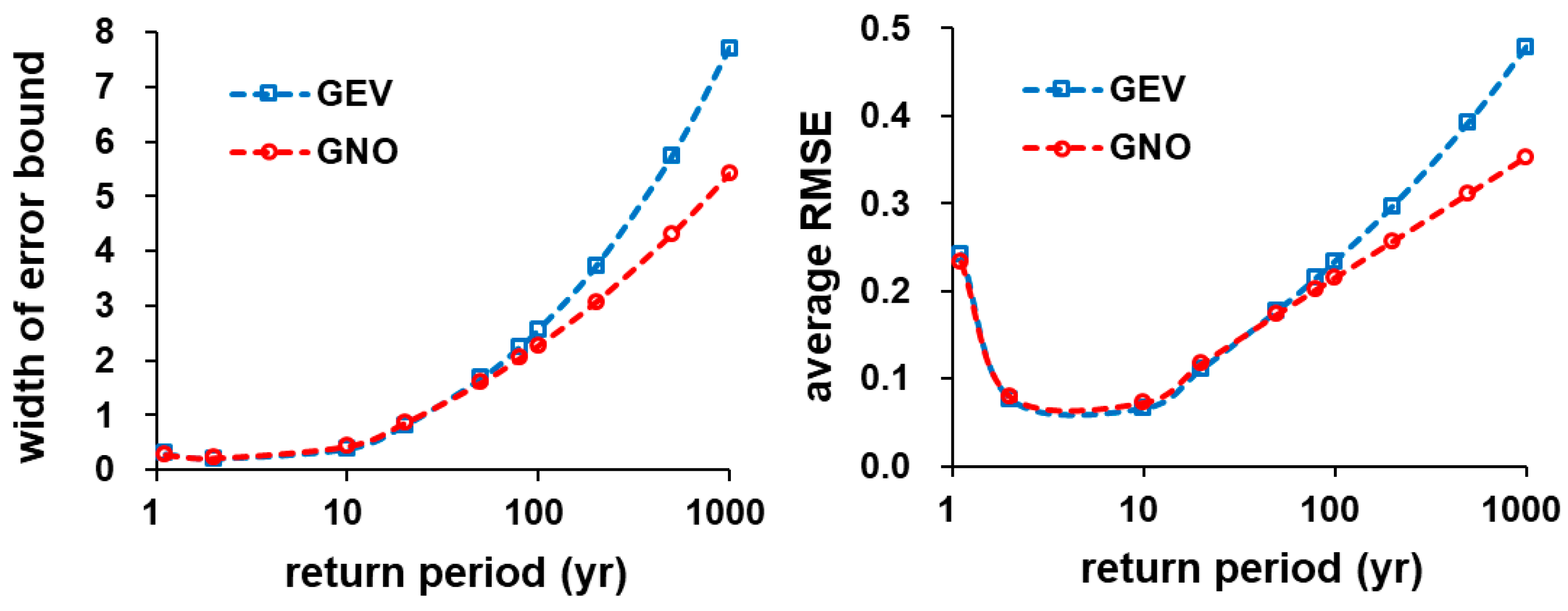
Figure 4 shows the regional growth curves with upper and lower error bounds. These error bounds were estimated by Equation (13). Figure 5 shows the widths of the error bounds and the regional average relative RMSE of the estimated growth curve computed by Equation (11). The widths of the error bounds and the regional average relative RMSE between GEV and GNO distributions were very similar for the return period smaller than 100 years. The width of the error bounds and the regional average relative RMSE of the GEV distribution becomes greater than that of the GNO distribution when the return period exceeds 100 years.
3.3. Assessment of Index Flood and Flood Quantiles
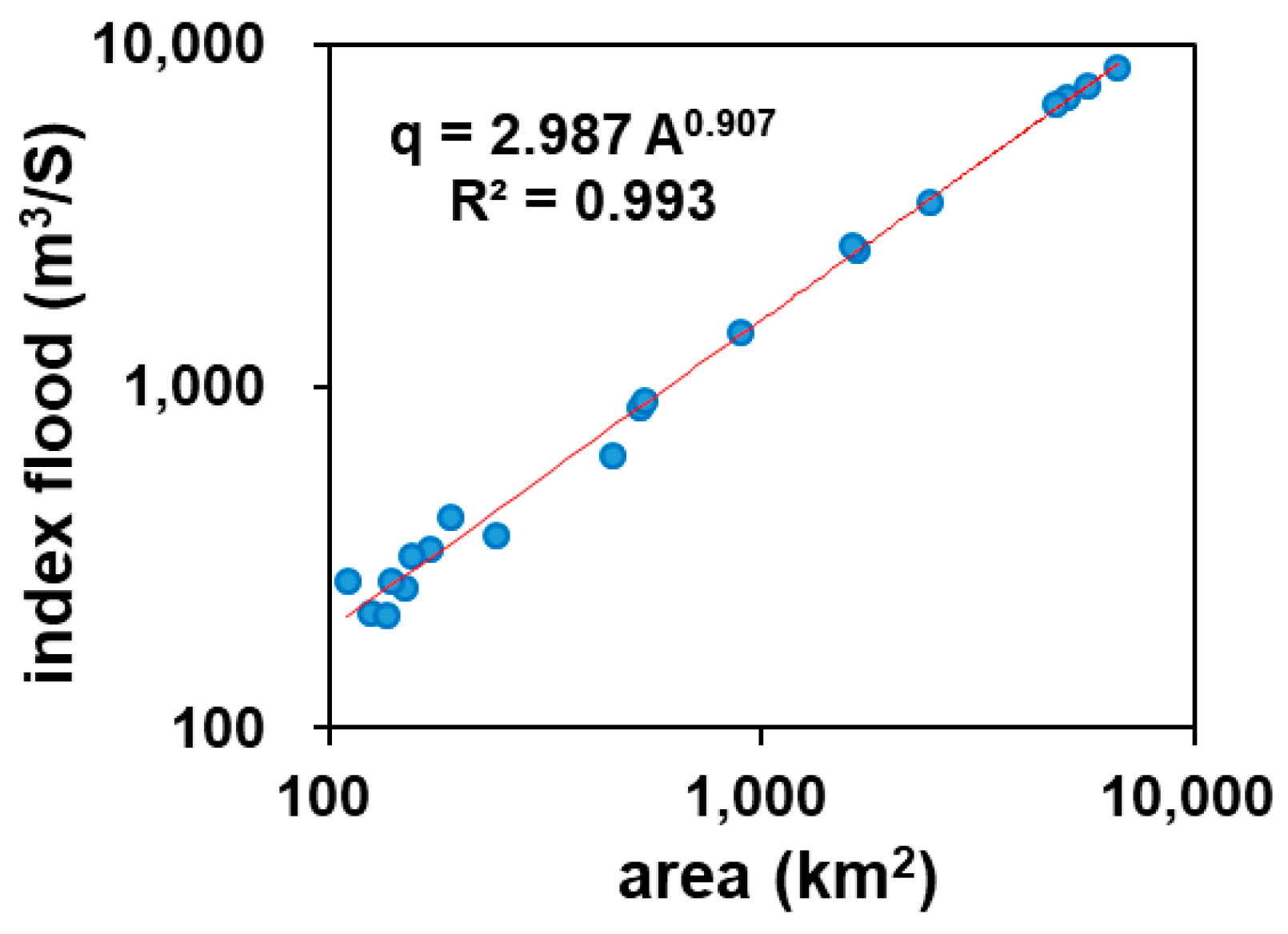
The index flood at any site can be estimated by averaging AMF data when the AMF data are available at a site. The index flood needs to be estimated indirectly for ungauged watersheds where AMF data are not available. In this study, the regionalized relation for the index flood was developed using the scale invariance properties of the index flood with respect to watershed area. The previous studies also applied the watershed area as the principal variable for predicting the index flood [14,39,40]. The power law equation for the index flood is represented by considering the first order moment of the peak discharge distribution within a homogeneous region [30].
In this equation, is the watershed area in km2, is a scaling exponent, and is the index flood associated with a unit watershed area. Using the simulated AMF data of 20 sites in Figure 1, the power law relation between and is determined as
Figure 6 shows the developed index flood relation and the coefficient of determination () is estimated as 0.99. Using the flood data generated from a storage function runoff model, Kim et al. [18] developed the following index flood relation in terms of watershed area.
The scaling exponent of this study was slightly higher than that of Kim et al. [18]. The index flood relations between this study and the previous study [18] are similar, and the differences in the index flood slightly increase as the watershed area decreases. Table 2 shows the relative errors between the observed and predicted index floods at the CJD and YC stations.
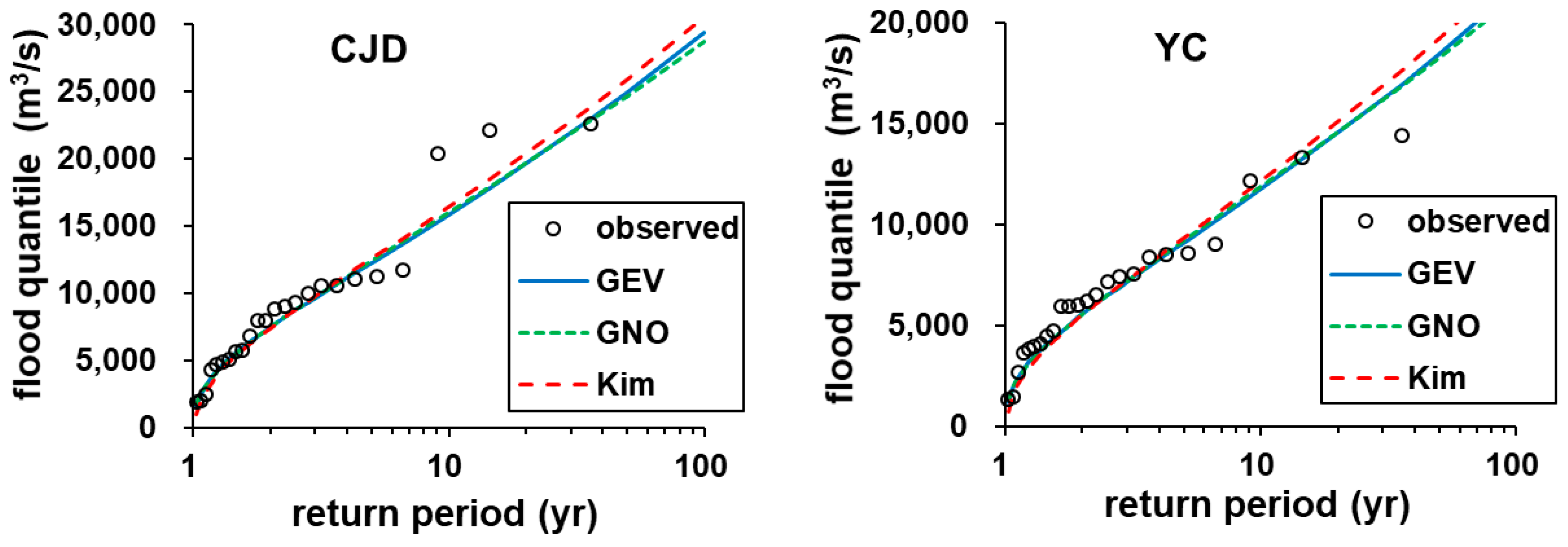
Figure 7 illustrates a comparison of the flood quantile relations at the CJD and YC stations. The flood quantiles were computed using Equation (6) with the developed index flood and growth curve. The probability of the ordered AMF data was estimated by the median plotting position formula described in Stedinger et al. [41]. The median plotting position formula was also applied by Kjeldsen et al. [12] to assess the proposed regional frequency distribution.
The predictive performance for the estimation of flood quantile was assessed using the CE and root mean square normalized error (RMSNE) statistic used in Salinas et al. [2]. Table 3 summarizes the CE and the RMSNE statistic for the estimation of flood quantiles at two locations. All cases exhibited satisfactory performance with CE values higher than 0.9. The RMSNE values predicted by this study were lower than those predicted by Kim et al. [17].
4. Discussion and Conclusions
We investigated the flood estimation method, which applies the combination of a rainfall-runoff simulation and the RFFA. The regional flood data were generated using the developed rainfall-runoff model. We tested the simulated flood responses at the outlet and one interior location in the basin. Due to the limited flood data, we could not test the simulated flood responses at other locations. The complete validation of a rainfall-runoff model is very difficult and might not be feasible in a poorly gauged basin. The rainfall-runoff model simulation might be the only alternative option for flood estimation in a poorly gauged basin even though the accuracy of the simulated flood data is uncertain. The simulation of a rainfall-runoff model contains various sources of uncertainty related to the inputs, model structures, model parameters, and initial conditions. These uncertainties have not been fully considered in this study. The methodology for uncertainty estimation of a rainfall-runoff model has been suggested in the literature [42]. Future research is needed to investigate the uncertainty related to how a rainfall-runoff model development affects the results of the RFFA.
The responses of simulated peak discharge based on the developed rainfall-runoff model were shown to be reasonable. The accuracy of peak discharge is a major concern for the present study rather than the accuracy of the entire hydrographs. Some observation related to the simulated hydrographs is briefly discussed. The satisfactory performance for large flood events might be related to the fact that the infiltration excess runoff mechanism becomes dominant. Consequently, the unit hydrograph method implemented in HEC-HMS was able to properly predict the runoff responses resulting from the infiltration excess runoff. The unsatisfactory performance for small and medium flood events might be due to a change in the dominant runoff processes. The dominant runoff process for small and medium flood events might change from the infiltration excess runoff to other runoff processes such as saturation excess overland flow or subsurface stormflow. It is well known that various runoff generation processes occur depending on the characteristics of rainfall, topography, soils, vegetation, and land use [43]. The previous studies demonstrated the change in the dominant runoff processes as the flood magnitude changes [44,45]. For the accurate simulation of hydrographs, it might be needed to consider the various runoff generation processes which the HEC-HMS cannot account for. For some storm events, the time to peak between the simulated hydrographs and the observed hydrographs are not consistent. This difference might be attributed to the inaccuracy of time of concentration specified in the simulation. We applied the empirical equation for time of concentration developed in the study basin, but the empirical equation might contain some uncertainty. The major parameters of the HEC-HMS affecting the flood responses are curve number, time of concentration, and storage coefficient. The poor performance of the simulated hydrographs for some storm events might be related to the misspecification of these parameters along with the incorrect runoff generation process considered in the simulation. In addition to the uncertainty of parameters and runoff processes, there is a need to investigate the uncertainty of the observed discharge data which affects the performance of simulation results.
The entire Chungju dam basin is considered as a homogeneous region based on the estimated discordancy and heterogeneity statistic. The regional average of sample L-moment ratios was the closest to the GEV distribution, and sample L-moment ratios were evenly dispersed through the GEV distribution. The examination of the L-moment diagram, statistic, and AWOD measure indicated that the GEV distribution was identified as the best fit to the simulated AMF data. This result is consistent with the previous study [17]. The difference of growth curves between GEV and GNO distributions grew slightly as the return period increased. The growth curves estimated from this study are slightly lower than that of Kim et al. [17]. However, the assessment of flood quantiles indicated that GEV and GNO distributions exhibited similar results such that it was difficult to identify the optimal regional frequency distribution. Further investigation is necessary for how to select the optimal regional frequency distribution among the candidate distributions. The widths of error bounds of the regional growth curve based on the GNO distribution were smaller than those based on the GEV distribution. The widths of error bounds estimated in the present study were comparable with the previous study [10]. There are different approaches for estimating the uncertainty bounds of the regional growth curve [46]. In future study, it might be meaningful to investigate the differences of uncertainty bounds of the regional growth curve between different approaches. The estimation of extreme flood quantiles was shown to be highly uncertain because the error bounds for the estimated growth curve significantly increased as the return period increased beyond 100 years.
The index flood was regionalized in terms of watershed area. The scaling exponent of the power law equation for the index flood was found to be around 0.9. The relative errors of the index flood evaluated at the CJD and YC stations were relatively small and the relative errors of the index flood for this study were smaller than those of the previous study [18]. The flood quantile estimates based on the simulated AMF data exhibited good agreement with those based on the observed AMF data. The estimated flood quantiles of this study are slightly better than those of the previous study [17] that were obtained for the same basin using a different rainfall-runoff model. The regional growth curves between this study and the previous study [17] were very similar although the location of sites used for the RFFA were different between two studies. This suggests that the results of RFFA are not largely affected by the choice of the sites used for the RFFA. The results of this study suggest that the flood estimation approach attempted in the present study might be a useful tool for the estimation of flood quantiles in the basin where the hourly rainfall data for major storm events are widely available and the observed flood data are sparse. The flood estimation method explored in this study is conceptually simple and involves less uncertain procedures compared with the design event approach, which transforms design rainfall into flood quantiles and has a wide application in engineering practice.
Supplementary Materials
The following are available online at https://www.mdpi.com/2073-4441/11/8/1717/s1, Figure S1: Observed and simulated hourly hydrographs for large flood events (a) the simulation period 5 August 2002 to 9 August 2002, (b) the simulation period 9 July 2006 to 19 July 2006. Figure S2: Observed and simulated hourly hydrographs for medium flood event (the simulation period 20 July 1987 to 25 July 1987). Figure S3: Observed and simulated hourly hydrographs for small flood event (the simulation period 17 August 2004 to 21 August 2004). Table S1: Simulation conditions and observed peak flow for each storm event. Table S2: Simulation results for each storm event.
Author Contributions
Conceptualization, N.W.K. and D.-H.L.; methodology, D.-H.L.; software, D.-H.L.; formal analysis, D.-H.L.; writing—original draft preparation, D.-H.L.; writing—review and editing, N.W.K. and D.-H.L.; funding acquisition, N.W.K.
Funding
This research was supported by the Strategic Research Project [project number 20180374] funded from Korea Institute of Civil Engineering and Building Technology.
Acknowledgments
The Authors are grateful to anonymous reviewers for their constructive comments and suggestion.
Conflicts of Interest
The authors declare no conflict of interest.
References
- GREHYS. Presentation and review of some methods for regional flood frequency analysis. J. Hydrol. 1996, 186, 63–84. [Google Scholar] [CrossRef]
- Salinas, J.L.; Laaha, G.; Rogger, M.; Parajka, J.; Viglione, A.; Sivapalan, M.; Blöschl, G. Comparative assessment of predictions in ungauged basins-Part 2: Flood and low flow studies. Hydrol. Earth Syst. Sci. 2013, 17, 2637–2652. [Google Scholar] [CrossRef]
- Ball, J.; Babister, M.; Nathan, R.; Weeks, W.; Weinmann, E.; Retallick, M.; Testoni, I. Australian Rainfall and Runoff: A Guide to Flood Estimation; Geoscience Australia: Canberra, Australia, 2019.
- Rahman, A.; Weinmann, P.E.; Hoang, T.M.T.; Laurenson, E.M. Monte Carlo simulation of flood frequency curves from rainfall. J. Hydrol. 2002, 256, 196–210. [Google Scholar] [CrossRef]
- Caballero, W.L.; Rahman, A. Development of regionalized joint probability approach to flood estimation: A case study for Eastern New South Wales, Australia. Hydrol. Process. 2014, 28, 4001–4010. [Google Scholar] [CrossRef]
- Blazkova, S.; Beven, K. Flood frequency estimation by continuous simulation for a catchment treated as ungauged (with uncertainty). Water Resour. Res. 2002, 38, 14-1–14-14. [Google Scholar] [CrossRef]
- Boughton, W.; Droop, O. Continuous simulation for design flood estimation—A review. Environ. Model. Softw. 2003, 18, 309–318. [Google Scholar] [CrossRef]
- Moretti, G.; Montanari, A. Inferring the flood frequency distribution for an ungauged basin using a spatially distributed rainfall-runoff model. Hydrol. Earth Syst. Sci. 2008, 12, 1141–1152. [Google Scholar] [CrossRef] [Green Version]
- Hosking, J.R.M.; Wallis, J.R. Regional Frequency Analysis: An Approach Based on L-Moments; Cambridge University Press: New York, NY, USA, 1997. [Google Scholar]
- Hussain, Z.; Pasha, G.R. Regional flood frequency analysis of the seven sites of Punjab, Pakistan, using L-moments. Water Resour. Manag. 2009, 23, 1917–1933. [Google Scholar] [CrossRef]
- Jingyi, Z.; Hall, M.J. Regional flood frequency analysis for the Gan-Ming River basin in China. J. Hydrol. 2004, 296, 98–117. [Google Scholar] [CrossRef]
- Kjeldsen, T.R.; Smithers, J.C.; Schulze, R.E. Regional flood frequency analysis in the KwaZulu-Natal province, South Africa, using the index-flood method. J. Hydrol. 2002, 255, 194–211. [Google Scholar] [CrossRef]
- Kumar, R.; Chatterjee, C.; Kumar, S.; Lohani, A.K.; Singh, R.D. Development of regional flood frequency relationships using L-moments for Middle Ganga Plains Subzone 1(f) of India. Water Resour. Manag. 2003, 17, 243–257. [Google Scholar] [CrossRef]
- Lim, Y.H.; Voeller, D.L. Regional flood estimations in Red river using L-Moment-based index-flood and bulletin 17B procedures. J. Hydrol. Eng. 2009, 14, 1002–1016. [Google Scholar] [CrossRef]
- Noto, L.V.; La Loggia, G. Use of L-moments approach for regional flood frequency analysis in Sicily, Italy. Water Resour. Manag. 2009, 23, 2207–2229. [Google Scholar] [CrossRef]
- Saf, B. Regional flood frequency analysis using L-moments for the west mediterranean region of Turkey. Water Resour. Manag. 2009, 23, 531–551. [Google Scholar] [CrossRef]
- Kim, N.W.; Lee, J.E.; Lee, J.W.; Jung, Y. Regional frequency analysis using spatial data extension method: I. An empirical investigation of regional flood frequency analysis. J. Korea Water Resour. Assoc. 2016, 49, 439–450. [Google Scholar] [CrossRef]
- Kim, N.W.; Lee, J.W.; Lee, J.; Lee, J.E. SWAT application to estimate design runoff curve number for South Korean conditions. Hydrol. Process. 2010, 24, 2156–2170. [Google Scholar] [CrossRef]
- Feldman, A.D. Hydrologic Modeling System HEC-HMS: Technical Reference Manual; U.S. Army Corps of Engineers Hydrologic Engineering Center: Davis, CA, USA, 2000.
- Aronica, G.T.; Candela, A. Derivation of flood frequency curves in poorly gauged Mediterranean catchments using a simple stochastic hydrological rainfall-runoff model. J. Hydrol. 2007, 347, 132–142. [Google Scholar] [CrossRef]
- Wagener, T.; Wheater, H.S.; Gupta, H.V. Rainfall-Runoff Modelling in Gauged and Ungauged Catchments; Imperial College Press: London, UK, 2004. [Google Scholar]
- Hrachowitz., M.; Savenije, H.H.G.; Blöschl, G.; McDonnell, J.J.; Sivapalan, M.; Pomeroy, J.W.; Arheimer, B.; Blume, T.; Clark, M.P.; Ehret, U.; et al. A decade of Predictions in Ungauged Basins (PUB)—A review. Hydrol. Sci. J. 2013, 58, 1198–1255. [Google Scholar] [CrossRef]
- Sivapalan, M. Prediction in ungauged basins: A grand challenge for theoretical hydrology. Hydrol. Process. 2003, 17, 3163–3170. [Google Scholar] [CrossRef]
- D’Asaro1, F.; Grillone, G. Empirical investigation of curve number method parameters in the Mediterranean area. J. Hydrol. Eng. 2012, 17, 1141–1152. [Google Scholar] [CrossRef]
- Woodward, D.E.; Hawkins, R.H.; Jiang, R.; Hjelmfelt, A.T.; Van Mullem, J.E.; Quan, Q.D. Runoff curve number method: Examination of the initial abstraction ratio. In Proceedings of the World Water and Environmental Resources Congress, Philadelphia, PA, USA, 23–26 June 2003. [Google Scholar] [CrossRef]
- USDA-Natural Resource Conservation Service (USDA-NRCS). National Engineering Handbook: Part 630 Hydrology; USDA: Washington, DC, USA, 2004.
- Lee, J.; Yoo, C.; Sin, J. Theoretical backgrounds of basin concentration time and storage coefficient and their empirical formula. J. Korea Water Resour. Assoc. 2013, 45, 155–169. [Google Scholar] [CrossRef]
- Pilgrim, D.H.; Cordery, I. Chapter 9 flood runoff. In Handbook of Hydrology; Maidment, D.R., Ed.; McGraw-Hill Inc.: New York, NY, USA, 1993; pp. 9.1–9.42. [Google Scholar]
- Dalrymple, T. Flood Frequency Analyses, Manual of Hydrology: Part 3; U.S. Government Printing Office: Washington, DC, USA, 1960.
- Bocchiola, D.; De Michele, C.; Rosso, R. Review of recent advances in index flood estimation. Hydrol. Earth Syst. Sci. 2003, 7, 283–296. [Google Scholar] [CrossRef] [Green Version]
- Greenwood, J.A.; Landwehr, J.M.; Matalas, N.C.; Wallis, J.R. Probability weighted moments: Definition and relation to parameters of several distributions expressible in inverse form. Water Resour. Res. 1979, 15, 1049–1054. [Google Scholar] [CrossRef]
- Mateus, A.; Caeiro, F. An R implementation of several randomness tests. AIP Conf. Proc. 2014, 1618, 531–534. [Google Scholar] [CrossRef]
- Mann, H.B. Nonparametric tests against trend. Econometrica 1945, 13, 245–259. [Google Scholar] [CrossRef]
- McCuen, R.H. Hydrologic Analysis and Design; Pearson Prentice Hall: Upper Saddle River, NJ, USA, 2005. [Google Scholar]
- Grubbs, F.; Beck, G. Extension of sample sizes and percentage points for significance tests of outlying observations. Technometrics 1972, 14, 847–854. [Google Scholar] [CrossRef]
- Hosking, J.R.M.; Wallis, J.R. Some statistics useful in regional frequency analysis. Water Resour. Res. 1993, 29, 271–281. [Google Scholar] [CrossRef]
- Kroll, C.N.; Vogel, R.M. Probability distribution of low streamflow series in the United States. J. Hydrol. Eng. 2002, 7, 137–146. [Google Scholar] [CrossRef]
- Cheng, K.S.; Lien, Y.T.; Wu, Y.C.; Su, Y.F. On the criteria of model performance evaluation for real-time flood forecasting. Stoch. Env. Res. Risk Assess 2017, 31, 1123–1146. [Google Scholar] [CrossRef]
- Kumar, R.; Chatterjee, C. Regional flood frequency analysis using L-moments for North Brahmaputra region of India. J. Hydrol. Eng. 2005, 10, 1–7. [Google Scholar] [CrossRef]
- Meigh, J.R.; Farquharson, F.A.K.; Sutcliffe, J.V. A worldwide comparison of regional flood estimation methods and climate. Hydrol. Sci. J. 1997, 42, 225–244. [Google Scholar] [CrossRef]
- Stedinger, J.R.; Vogel, R.M.; Foufoula-Georgiou, E. Chapter 18 Frequency analysis of extreme events. In Handbook of Hydrology; Maidment, D.R., Ed.; McGraw-Hill Inc.: New York, NY, USA, 1993; pp. 18.1–18.66. [Google Scholar]
- Beven, K.; Binley, A. GLUE: 20 years on. Hydrol. Process. 2014, 28, 5897–5918. [Google Scholar] [CrossRef]
- Beven, K.J. Rainfall-Runoff Modelling: The Primer; John Wiley & Sons, Ltd.: Chichester, UK, 2001. [Google Scholar]
- Jothityangkoon, C.; Sivapalan, M. Towards estimation of extreme floods: Examination of the roles of runoff process changes and floodplain flows. J. Hydrol. 2003, 281, 206–229. [Google Scholar] [CrossRef]
- Sivapalan, M.; Wood, E.F.; Beven, K.J. On hydrologic similarity. 3. A dimensionless flood frequency model using a generalised geomorphic unit hydrograph and partial area runoff generation. Water Resour. Res. 1990, 26, 43–58. [Google Scholar] [CrossRef]
- Hailegeorgis, T.T.; Alfredsen, K. Regional flood frequency analysis and prediction in ungauged basins including estimation of major uncertainties for mid-Norway. J. Hydrol. Reg. Stud. 2017, 9, 104–126. [Google Scholar] [CrossRef]
Figure 1.
The Chungju dam basin and sites used for the RFFA (left). The divided sub-watershed is based on water resource unit map defined in WAMIS (www.wamis.go.kr).
Figure 1.
The Chungju dam basin and sites used for the RFFA (left). The divided sub-watershed is based on water resource unit map defined in WAMIS (www.wamis.go.kr).

Figure 2.
Comparison of observed AMF and simulated AMF. R indicates the coefficient of correlation and CE indicates the coefficient of efficiency. The blue dotted line indicates 1:1 line.
Figure 2.
Comparison of observed AMF and simulated AMF. R indicates the coefficient of correlation and CE indicates the coefficient of efficiency. The blue dotted line indicates 1:1 line.

Figure 3.
L-moment ratio diagram (left) and the comparison of regional growth curves (right). Kim is the result of Kim et al. [17].
Figure 3.
L-moment ratio diagram (left) and the comparison of regional growth curves (right). Kim is the result of Kim et al. [17].

Figure 4.
Regional growth curves with 90% error bounds. GEV distribution (left); GNO distribution (right).
Figure 4.
Regional growth curves with 90% error bounds. GEV distribution (left); GNO distribution (right).

Figure 5.
Width of error bounds and regional average relative RMSE of the estimated growth curves. width of error bounds (left); regional average relative RMSE (right).
Figure 5.
Width of error bounds and regional average relative RMSE of the estimated growth curves. width of error bounds (left); regional average relative RMSE (right).

Figure 6.
Index flood relation.

Figure 7.
Comparison of flood quantiles. Kim is the result of Kim et al. [17].
Figure 7.
Comparison of flood quantiles. Kim is the result of Kim et al. [17].


Table 1.
Goodness-of-fit and AWOD statistics for candidate distributions.
| Distribution | Z Value | AWOD |
|---|---|---|
| GLO | 0.71 | 0.0321 |
| GEV | −0.66 | 0.0261 |
| GNO | −1.31 | 0.0284 |
| PE3 | −2.5 | - |
| GP | −4.11 | - |
Table 2.
Comparison of relative errors for index flood.
| Station | This Study | Kim |
|---|---|---|
| CJD | 3.24% | 6.46% |
| YC | 1.03% | 3.24% |
* Kim is based on the result of Kim et al. [18].
Table 3.
CE and RMSNE statistic for the estimation of flood quantile.
| Station | GEV | GNO | Kim |
|---|---|---|---|
| CJD | 0.92 (0.13) | 0.93 (0.13) | 0.93 (0.15) |
| YC | 0.94 (0.13) | 0.94 (0.13) | 0.91 (0.17) |
* The values in the parenthesis indicate RMSNE. Kim is based on the result of Kim et al. [17].
© 2019 by the authors. Licensee MDPI, Basel, Switzerland. This article is an open access article distributed under the terms and conditions of the Creative Commons Attribution (CC BY) license (http://creativecommons.org/licenses/by/4.0/).
Share and Cite
MDPI and ACS Style
Lee, D.-H.; Kim, N.W. Regional Flood Frequency Analysis for a Poorly Gauged Basin Using the Simulated Flood Data and L-Moment Method. Water 2019, 11, 1717. https://doi.org/10.3390/w11081717
AMA Style
Lee D-H, Kim NW. Regional Flood Frequency Analysis for a Poorly Gauged Basin Using the Simulated Flood Data and L-Moment Method. Water. 2019; 11(8):1717. https://doi.org/10.3390/w11081717
Chicago/Turabian StyleLee, Do-Hun, and Nam Won Kim. 2019. "Regional Flood Frequency Analysis for a Poorly Gauged Basin Using the Simulated Flood Data and L-Moment Method" Water 11, no. 8: 1717. https://doi.org/10.3390/w11081717
Note that from the first issue of 2016, this journal uses article numbers instead of page numbers. See further details here.