Assessing the Efficiency of Alternative Best Management Practices to Reduce Nonpoint Source Pollution in a Rural Watershed Located in Louisiana, USA

Abstract

We conducted biophysical simulations using MapShed to determine the effects of adopting best management practices (BMPs) to reduce nutrients and sediment pollution in a watershed dominated by poultry production in the Saline Bayou Watershed, Louisiana, USA. The reduction of three water pollutants, nitrogen, phosphorus, and sediment from adopting different BMPs were assessed using a linear programming model with the cost minimization objective. We considered three weather scenarios (dry, normal, and wet) and BMP parameter efficiencies obtained from linear regression models. Optimization results showed that nutrient management and agricultural land retirement reduced most of the phosphorus runoff in the watershed at the lowest cost. Results were robust to alternative weather (dry, normal, and wet) scenarios.

1. Introduction

Agriculture activities are a leading cause of nonpoint source (NPS) pollution in the USA [1]. Nonpoint source pollution in Louisiana’s rural watersheds comes primarily from row crop agriculture and repetitive application of poultry manure on the same parcel of land located in or around watershed close to poultry farms [2]. These practices have resulted in nutrient runoff and leaching and sediment runoff to nearby water bodies. Realizing the difficulty of regulating nonpoint sources of pollution from agriculture, the United States Department of Agriculture/Natural Resource Conservation Service (USDA/NRCS) has proposed that farmers adopt best management practices (BMPs). These BMPs are adopted on a voluntary basis with a certain percentage of cost share provided by the USDA/NRCS based on the land characteristics (a complex scoring system reflecting land characteristics) and economic wellbeing of farmers (based on whether a farmer is a limited resources farmer or not) [3]. With the implementation of the total daily maximum load rule by the United States Environmental Protection Agency, there is a certain water quality standard that each water segment must meet. Though there are several ways to meet this standard in an agriculturally dominated watershed, one of the best ways is through the voluntary adoption of BMPs by farmers.

Statistics from the Environmental Protection Agency (EPA) reveal that about 28% of reservoirs and 17% of the river systems in the United States are classified as nutrient-impaired and need immediate action to improve water health [4]. Similarly, based on the biological condition measuring the physical and physical components of water, the US EPA (2016) [5] has found that 46% of nation’s streams are in poor condition. The impairment of the water is due to the accumulation of nutrients and sediment. Nutrient and sediment accumulations could cause serious problems, such as oxygen deficiency and poor water quality unsuitable for recreation, drinking, and agricultural and industrial uses [6]. Good watershed management leads to effective management practices to protect water resources [7]. Past efforts have been mainly focused on the management and control of point pollution, while non-point pollution control has not been properly addressed because of difficulty of identifying its spatial distribution and temporal variation [6]. Agricultural runoff is a significant contributor to nonpoint source pollution in rural areas, and it contributes about 65% of the nitrogen pollution to the Gulf of Mexico [8]. Each part of the watershed plays its own role in nutrient and sediment contribution, which depends on its physiographic structure, such as soil type, land use and land cover, and gradient. Some areas contribute more to nutrient and sediment pollution in a given watershed, and these areas are known as critical source areas (CSAs). These areas are extremely important from the economic point of view for watershed management. There are numerous studies on nonpoint source pollution reduction [9,10] that recommend identifying CSAs for cost effective pollution management in a watershed. Such areas could be identified by water monitoring from the sub-watershed level or by a simulation model, or a combination of both [11]. Direct sub-watershed monitoring is not feasible, because it is labor intensive, time consuming and financially prohibitive. An alternative to monitoring is to use watershed models, such as the Soil and Water Assessment Tool (SWAT) [12] and the Generalized Watershed Loading Function (GWLF) [13]. These models avoid some limitations of field study and help to identify and prioritize watersheds for cost effectiveness of BMPs practices [14,15].

The SWAT has been widely used in different parts of the world for the identification and prioritization of CSAs [14,15,16,17,18,19,20]. It has also been used for predicting stream flow, nutrients, and sediment from watersheds [21,22,23,24]. We use MapShed as it is an open source MapWindow (http://www.mapshed.psu.edu/)-based model. The MapShed and its precursor the ArcView Generalized Watershed Loading Function (AVGWLF) model has been widely used to identify CSAs and to simulate stream flow, nitrogen, and phosphorus loading [9]. MapShed combines hydrology, land cover, soils, topography, weather, pollutant discharges, and other data to determine the amount of nutrient and sediment transport in a given watershed. We simulated the effects of alternative BMPs to reduce nutrient and sediment pollution within the Saline Bayou watershed in Louisiana, USA, which is dominated by poultry operations. Our objectives were to:

(1)

Simulate the effects of different best management practices to reduce nitrogen, phosphorus, and sediment in the Saline Bayou watershed by using MapShed, and

(2)

Determine the most cost effective combination of best management practices under alternative phosphorus reduction goals with dry, normal, and wet weather situations.

2. Study Area

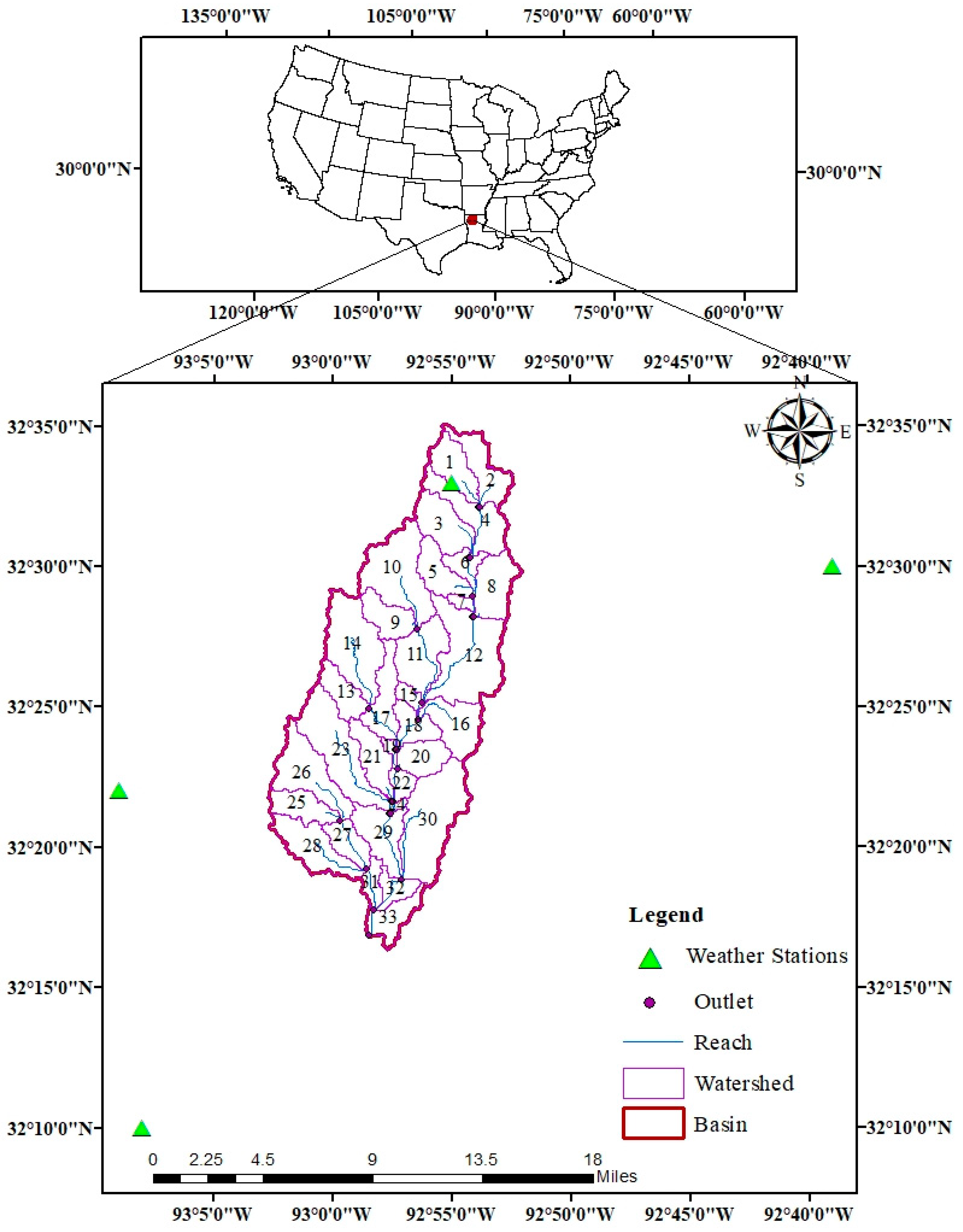
We chose Saline Bayou Watershed (HUC 11140208), located in Bienville and Lincoln Parishes (counties), Louisiana (Figure 1). The Louisiana Department of Environmental Quality (LDEQ) listed it as one of the priority watersheds to be comprehensively studied with respect to BMP adoptions. The watershed is located between longitude 92°52′01′′ and 93°04′44′′ W and latitude 32°14′49′′ and 32°34′48′′ N. Its area is 383.81 square km of relatively flat land, varying from 46 m to 163 m above the sea level. The total length of the streams in this area is 66.4 km, out of which 3.3 km of the streams lies inside the agricultural area. This watershed has a heavy concentration of the poultry production in Louisiana. The watershed area is dominated by a temperate climate, with temperatures ranging from −2.2 °C (min) to 40.5 °C (max). In the two parishes where the watershed is located, vegetable crops, hay, and timbers are prevalent although adjoining parishes grow row crops such as corn, cotton, rice, soybeans, and wheat.

3. Modeling Approach

We utilized MapShed [13] to obtain N, P, and sediment runoff under alternative BMP adoption scenarios. The model divided the watershed into 33 sub-watersheds for better representing the sub-watershed characteristics on the pollutant discharge. Calibration and validation of the model were done by using the discharge data of the United States Geological Survey (USGS) gaging station located at the outlet of sub-watershed number 33 (see Figure 1).

The MapShed model is embedded with the AVGWLF, which generates all the necessary information to run the model. This GWLF model can simulate runoff, nutrients, and sediment from different watersheds. This model simulates runoff by a water-balance technique based on daily precipitation, daily temperature, land use, and soil data. This model is known to be a distributed/lumped parameter model because of its characteristics of distributing the surface loading by taking various land use covered scenarios while, for a lumped parameter model, it takes sub-surface loading. In the GWLF, precipitation is separated between direct runoff and infiltration by using a form of the Natural Resource Conservation Service’s (NRCS) Curve Number (CN) method [25,26]. Erosion and sediment yield are computed in the MapShed based on the Universal Soil Loss Equation (USLE). The sediment delivery ratio, which is the key factor for computing sediment yield, is based on the watershed size and transport capacity. The daily runoff volume that transports sediment is computed by using the CN, which is a function of soil and land use/cover. Dissolved nutrient load and sediment transporting through rural areas are computed by multiplying their respective coefficients with runoff. In the GWLF, all the N and P from the urban areas are considered to be in a solid state, and the model uses exponential accumulation and wash-off function for an estimation of urban loading. The sub-surface losses in the watershed are estimated by using dissolved N and P concentrations, where the watershed is considered to be single lumped-parameter contributing area [13].

4. Data

The necessary input data layers needed for MapShed were collected from various sources (

Table 1. Information of hydrological, meteorological, and other data used in the research.

Station ID	Type	Longitude	Latitude	Elevation (m asl)	Duration
160277	Rainfall/Temperature	92.917	32.550		2001	2010
168067	Rainfall/Temperature	92.650	32.550		2001	2010
164288	Rainfall/Temperature	93.383	32.167		2001	2010
168094	Rainfall/Temperature	93.150	32.367		2001	2010
735200	Discharge	92.976	32.250	45.540	2001	2010

). Since this was a Geographical Information System (GIS)-based model, several raster and vector data were needed to run the model. Watershed and parishes boundaries were extracted from the Louisiana water mapping service (http://sslmaps.tamu.edu/website/srwp/Louisiana/viewer.htm). The DEM, which is requisite data for calculating slope related information used in the model, was obtained from the Louisiana GIS CD (\\gid-store.lsu.edu\gis). The land use/cover is a raster layer, which helps to estimate nutrient flows throughout the watershed, is obtained from the Louisiana Atlas data portal (http://atlas.lsu.edu). The stream layer is obtained from the USGS site. The physiographic provinces (polygon) layer contains the area with hydraulic parameters, such as the warm rain erosion rate, the cool rain erosion rate, and the groundwater recession rate, and was digitized from the USGS map of physiographic regions compatible with the MapShed model. The animal feeding operation (AFO) layer is used to describe the animal population. The total animals in the watershed are obtained from the LSU Agricultural five-year summary, which provide agricultural data for 2006–2010. The average of the five-year animal census minimizes the yearly fluctuation of animals in a parish of an individual year. The most recent animal census is selected for the study. The soil layer, which is one of the most important inputs for the MapShed model, show the hydraulic properties, erodibility factor, and water holding capacity. The MapShed model requires both raster and vector data of the soil, and this is obtained from the Louisiana GIS center. We use information from the four most close by NOAA weather stations to the watershed to better represent the daily precipitation and maximum and minimum temperature of the entire watershed (http://www.ncdc.noaa.gov/cdo-web/search).

5. BMP Reduction Coefficients and the Optimization Technique

We considered eight BMPs for their ability to reduce nitrogen, phosphorus and sediment pollution. These eight BMPs were Cover Crops (BMP₁), Conservation Tillage (BMP₂), Conservation Plan (BMP₃), Nutrient Management (BMP₄), Agland Retirement (BMP₅), Stream Length with Vegetated Buffer Strips (BMP₆), Stream Length with Fencing (BMP₇), and Stream length with Bank Stabilization (BMP₈). BMP reduction coefficients determine the BMP’s effectiveness at reducing N, P, and sediment and indicate the amount of nutrients or sediment reduction by one unit (hectare for the watershed area and meter for the stream-based BMPs) increase in BMP adoption. To get the coefficients of each BMP, regression analyses were carried out on simulated output. The simulation outputs were subtracted from the baseline output (no BMP adoption) to obtain the amount of nutrient reduction at each level for the adopted BMP. The coefficients of BMP₆, BMP₇, and BMP₈ were calculated by varying one unit of stream length, while the coefficients of the remaining BMPs were calculated by varying 2% of corresponding BMPs values. Regression analyses were performed between the amounts of nutrient reduction for each level of adoption and the amount of land associated with each level, which gives the nutrient reduction coefficient. These coefficients indicate how many units of nutrient or sediment are reduced per unit of land.

An optimization model developed to determine the land cover at least cost and at different levels of pollution is shown below (Equations (1)–(6)). The objective of this optimization model was to achieve the maximum pollution reduction at the lowest cost. To achieve such a goal, constraints were placed on resources and minimum requirements for nutrient reduction rates. Phosphorus was taken as a primary nutrient for reduction because of its prime role in surface water pollution, eutrophication and hypoxia in the Gulf of Mexico. Similarly, nitrogen and sediment reduction were taken as secondary goals. In each watershed and dry and wet years, various levels of phosphorus reduction were analyzed.

$$Min {\displaystyle \sum }_{i=1}^j{c}_i{B}_i$$

(1)

$\mathrm{Subject}\mathrm{to}$

$$Nitrogen:{\displaystyle \sum }_{i=1}^j{n}_i{B}_i\ge 0$$

(2)

$$Sediment:{\displaystyle \sum }_{i=1}^j{s}_i{B}_i\ge 0$$

(3)

$$Phosphorus:{\displaystyle \sum }_{i=1}^j{p}_i{B}_i\ge \alpha I_p$$

(4)

$$Other: {\displaystyle \sum }_{i=1}^j{o}_{i,k}{B}_i\le R_k,for all k= 1,\dots \dots ,K$$

(5)

$$B_i\ge 0$$

(6)

$\mathrm{where}: c_i=Cost of BMP i$

• $B_i=i^{th}BMP$
• $s_i=Sediment reduced by i^{th}BMP$
• $n_i=Nitrogen reduced by i^{th}BMP$
• $p_i=Phosphorus reduced by i^{th}BMP$
• $\alpha =desired fraction of total phosphorus reduction (0<\alpha \le 1)$
• $I_p=Total phosphorus loading without BMP adoption$
• $o_{i,k}=Land unit covered by BMP i for land use k$
• $R_k=Maximum allowable land useage for use k$

Technical coefficients ($n_i$, $p_i$, $s_i$) and objective function coefficients ($c_i)$ used in the model are shown in

Table 2. Objective function coefficients (c_i) and technical coefficients ($n_i$, $p_i$, $s_i$) used in the optimization model (Normal weather scenario).

Parameters	Cover Crop	Conservation Tillage	Conservation Crop Rotation	Nutrient Management Plan	Agland Retirement	Vegetative Buffer	Fencing	Streambank Stabilization
$c_i$ ($/ha or $/m)	182.32	71.93	26.82	41.57	152.98	18.88	5.62	86.38
$n_i$ (kg/ha)	3.11	0.86	0.54	5.05	16.43	0.41	0.01	0.02
$p_i$ (kg/ha)	1.83	0.81	0.37	1.67	3.48	0.12	0.01	0.01
$s_i$ (tons/ha)	0.37	0.32	0.17	0.00	1.02	0.05	0.03	0.04

Notes: Cost is given in U.S. dollars here and all through the paper.$n_i$, $p_i$, $s_i$ denote nitrogen, phosphorus, and sediment reduced by adopting $i^{th}BMP$, respectively. ‘ha’ stands for hectare, ’m’ stands for meter.

.

Calibration and Validation

Visual inspection between the measured and simulated hydrograph is an easy way to evaluate model performance. Various statistical criteria are available for numerical evaluation of model performance. Nevertheless, adopting many evaluation criteria for the model’s performance increases unnecessary burdens for potential users. Therefore, only four model performance evaluation statistics were used; the Nash–Sutcliffe Efficiency (NSE), percent bias (PBIAS), ratio of root mean square error (RMS), and the coefficient of determination (R²).

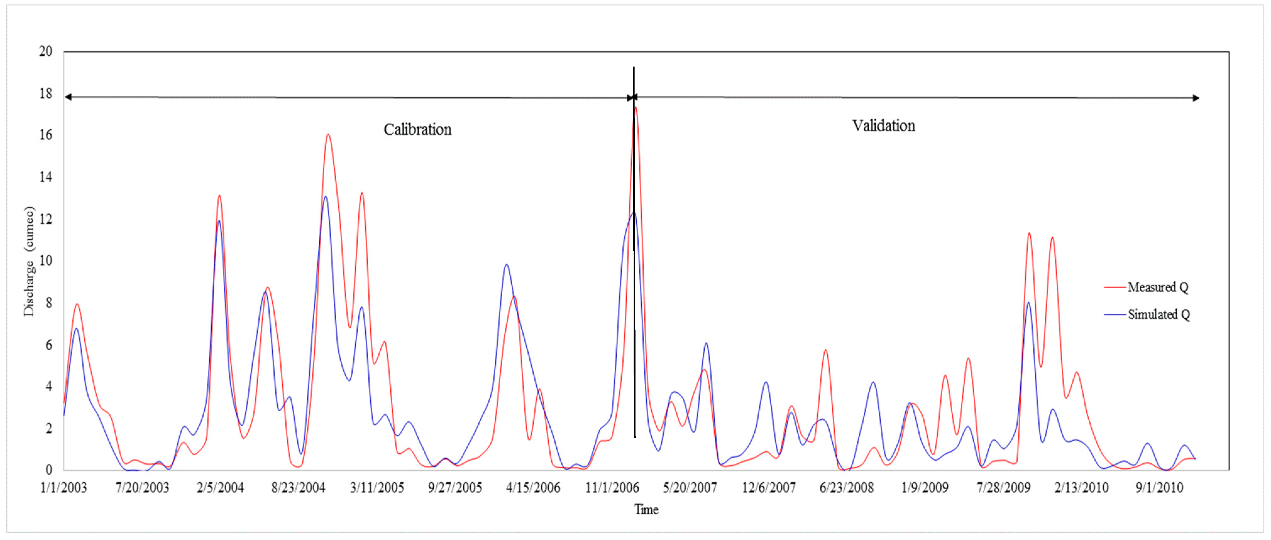
Discharge data for the Saline Bayou outlet was obtained from the United Stated Geological Survey (USGS) for 2001–2010 for calibration and validation of the model. To understand the uncertain character of the watershed, data from 2001 to 2002 were used for a warm-up period, data from 2003–2006 were used for calibration, and the remaining data were used for validation. The MapShed model was able to predict monthly flow data with good accuracy, which was shown by four performance evaluation statistics: NSE = 70%, PBIAS = 0.00, RMS = 0.55, and R² = 0.70 for the calibration and NSE = 59%, PBIAS = 0.21, RMS = 0.64, and R² = 0.64 for validation. Generally, model simulation is considered to be satisfactory if NSE > 0.5, RMS < 0.70, PBIAS ± 25% for stream flow [27]. Our results satisfy these constraints; therefore, MapShed performed well. Figure 2 shows the graphical representation of the calibration and validation result.

The manual calibration technique was adopted. Various parameters were changed within their range in order to get the best fit with the observed data (

Table 3. Calibrated parameters of the MapShed model.

Parameters	Definition	Default Value	Calibrated Values
Curve number (CN) Cropland Forest Wetland	Predicts direct runoff or infiltration from effective rainfall based on soil and land cover	Varies	80 75 85
Groundwater recession Coefficient (ALPHA_BF)	Indicates the interaction between groundwater and surface water systems.	0.1	0.07
Seepage coefficient (GW_REVAP)	Indicates the fraction of infiltrated water that goes to an underlying aquifer	0	0.05
Erodibility factor (K) Cropland Forest Wetland	Indicates the susceptibility of soil to erode and the rate of runoff	0.05–0.65	0.41 0.40 0.42
Slope length factor (LS) Cropland Forest Wetland	Indicates the effect of slope length on erosion which is a function of overland runoff and slope		0.25 0.39 0.00
Cropping management factor (C) Cropland Forest Wetland	Indicates the effect of cropping and management practice on erosion rates	0.002–0.3	0.42 0.002 0.01
Available water cap			0.411

). Curve numbers (CN1, CNP, and CN) were empirical parameters used to predict direct runoff or infiltration from effective rainfall based on soil and land cover. The soil erodibility factor (K) indicates the susceptibility of soil to erode and the rate of runoff. The clay soil has a high K value because of the high value of resistance to detachment. The slope length factor (LS) indicates the effect of slope length on erosion, which is a function of overland runoff and slope. The cropping management factor (C) indicates the effect of cropping and management practices on erosion rates. This factor is most often used to see the impact of management on a conservation plan. Evapotranspiration (ET) measures the evaporation from the soil transpired through the plants, which is a function of the number of daylight hours, which are calculated using the latitude of the centroid of a given watershed, saturated water vapor pressure, and the mean daily temperature on a given day. The Groundwater Seepage Coefficient represents the fraction of infiltrated water that goes to an underlying aquifer. The Groundwater Recession Coefficient is used to characterize the interaction between groundwater and surface systems.

6. Results from an Optimization Model

Optimization results were obtained for various levels (

Table 4. Summary of best management practice (BMP) adopted area, total cost of pollutant reduction, and unit cost of nitrogen, phosphorus, and sediment reductions under alternative weather scenarios in the Saline Bayou watershed (normal weather scenario (2002–2009)).

Scenario	Cover Crops (BMP1) in hectare	Conservation Tillage (BMP2) in hectare	Conservation Plan (BMP3) in hectare	Nutrient Management (BMP4) in hectare	Agland Retirement (BMP5) in hectare	Vegetative Buffer (BMP6) in meter	Fencing (BMP7) in meter	Streambank Stabilization (BMP8) in meters	Total Cost ($)	N Level Reduced (kg)	P Level Reduced (kg)	Sediment Level Reduced (tons)	Cost($) of N Reduction per kg	Cost ($) of P Reduction per kg	Cost($) of Sediment Reduction per ton
10%	0.00	0.00	0.00	28.81	0.00	0.00	0.00	0.00	1197.63	145.39	48.04	0.000	8.24	24.93	Undefined
20%	0.00	0.00	0.00	57.61	0.00	0.00	0.00	0.00	2394.85	290.78	96.08	0.000	8.24	24.93	Undefined
30%	0.00	0.00	0.00	86.42	0.00	0.00	0.00	0.00	3592.48	436.16	144.12	0.000	8.24	24.93	Undefined
40%	0.00	0.00	0.00	90.90	10.10	44.24	0.00	0.00	6159.06	642.81	192.16	12.360	9.58	32.05	498.31
50%	56.40	0.00	0.00	34.50	10.10	360.00	0.00	0.00	20058.91	662.83	245.20	48.520	30.26	81.81	413.42
51% (max)	86.05	0.00	0.00	4.85	10.10	360.00	0.00	0.00	24232.15	605.51	245.00	59.610	40.02	98.91	406.51

Notes: Column heading labeled “Scenario” shows the desired level of phosphorus reduction from the base level (when no BMPs are adopted). Therefore, it is only possible to reduce the maximum of 51% of phosphorus from the base level at the dry weather scenario. Values under each BMP shows the area on which this BMP was adopted. Total cost indicates the cost of reducing a given % of phosphorus from the base level, which also reduces a certain amount of nitrogen and sediment. The amount of N, P, and sediment reduction are shown under the N level reduced, P level reduced, and sediment level reduced. Unit cost shows the cost of reducing N, P, or sediment. Cost is given in U.S. dollars.

,

Table 5. Summary of BMP adopted area, total cost of pollutant reduction, and unit cost of nitrogen, phosphorus, and sediment reductions under alternative weather scenarios in the Saline Bayou watershed (wet year (2001)).

Scenario	Cover Crops (BMP1) in hectare	Conservation Tillage (BMP2) in hectare	Conservation Plan (BMP3) in hectare	Nutrient Management (BMP4) in hectare	Agland Retirement (BMP5) in hectare	Vegetative Buffer (BMP6) in meter	Fencing (BMP7) in meter	Streambank Stabilization (BMP8) in meters	Total Cost ($)	N Level Reduced (kg)	P Level Reduced (kg)	Sediment Level Reduced (tons)	Cost($) of N Reduction per kg	Cost ($) of P Reduction per kg	Cost($) of Sediment Reduction per ton
10%	0.00	0.00	0.00	27.97	0.00	0.00	0.00	0.00	1162.71	230.03	75.36	0	5.05	15.43	Undefined
20%	0.00	0.00	0.00	55.93	0.00	0.00	0.00	0.00	2325.01	460.05	150.72	0	5.05	15.43	Undefined
30%	0.00	0.00	0.00	83.90	0.00	0.00	0.00	0.00	3487.72	690.08	226.08	0	5.05	15.43	Undefined
40%	0.00	0.00	0.00	91.09	9.91	44.24	0.00	0.00	6137.89	1014.57	301.44	14.42	6.05	20.36	425.65
50%	9.80	0.00	0.00	81.10	10.10	360.00	0.00	0.00	13499.96	1255.68	376.8	44.53	10.75	35.83	303.17
51% (max)	90.86	0.00	0.00	0.04	10.10	360.00	0.00	0.00	24909.16	1051.53	399.41	87.95	23.69	62.36	283.22

Notes: Column heading labeled “Scenario” shows the desired level of phosphorus reduction from the base level (when no BMPs are adopted). Therefore, it is only possible to reduce the maximum of 51% of phosphorus from the base level at the dry weather scenario. Values under each BMP shows the area on which this BMP was adopted. Total cost indicates the cost of reducing a given % of phosphorus from the base level, which also reduces a certain amount of nitrogen and sediment. The amount of N, P, and sediment reduction are shown under the N level reduced, P level reduced, and sediment level reduced. Unit cost shows the cost of reducing N, P, or sediment. Cost is given in U.S. dollars.

and

Table 6. Summary of BMP adopted area, total cost of pollutant reduction, and unit cost of nitrogen, phosphorus, and sediment reductions under alternative weather scenarios in the Saline Bayou watershed (Dry Year (2010)).

Scenario	Cover Crops (BMP1) in hectare	Conservation Tillage (BMP2) in hectare	Conservation Plan (BMP3) in hectare	Nutrient Management (BMP4) in hectare	Agland Retirement (BMP5) in hectare	Vegetative Buffer (BMP6) in meter	Fencing (BMP7) in meter	Streambank Stabilization (BMP8) in meters	Total Cost ($)	N Level Reduced (kg)	P Level Reduced (kg)	Sediment Level Reduced (tons)	Cost($) of N Reduction per kg	Cost ($) of P Reduction per kg	Cost($) of Sediment Reduction per ton
10%	0.00	0.00	0.00	33.75	0.00	0.00	0.00	0.00	1402.99	62.32	36.95	0	22.51	37.97	Undefined
20%	0.00	0.00	0.00	67.50	0.00	0.00	0.00	0.00	2805.98	124.65	73.9	0	22.51	37.97	Undefined
30%	0.00	0.00	0.00	100.75	0.25	0.00	0.00	0.00	4226.42	187.54	120.85	0.091	22.54	34.97	46444.20
40%	59.66	0.00	0.00	31.24	10.10	360.00	0.00	0.00	20517.76	195.24	217.8	24.824	105.09	94.20	826.53
41% (max)	90.90	0.00	0.00	0.00	10.10	360.00	360.00	0.00	26937.99	158.85	249.49	30.413	169.58	107.97	885.74

Notes: Column heading labeled “Scenario” shows the desired level of phosphorus reduction from the base level (when no BMPs are adopted). Therefore, it is only possible to reduce the maximum of 41% of phosphorus from the base level at the dry weather scenario. Values under each BMP shows the area on which this BMP was adopted. Total cost indicates the cost of reducing a given % of phosphorus from the base level, which also reduces a certain amount of nitrogen and sediment. The amount of N, P, and sediment reduction are shown under the N level reduced, P level reduced, and sediment level reduced. Unit cost shows the cost of reducing N, P, or sediment. Cost is given in U.S. dollars.

) of desired phosphorus reduction under normal, wet, and dry weather conditions. The baseline nutrients and sediment loading in the watershed without adopting any BMPs were 5.5 tons of nitrogen, 0.48 tons of phosphorus, and 144 tons of sediment. In the wet weather scenario, higher amounts of nutrients and sediment could be reduced effectively by adopting BMPs. In the dry weather scenario, BMPs did not reduce nutrient load as much as they did in normal or wet weather scenarios. This outcome could be attributed to rainfall and runoff situations as the lack of sufficient rainfall results in less runoff and less nutrient loading.

Nutrient management was the preferred BMP in a normal weather scenario. It could reduce up to 30% of the phosphorus load from the watershed at the cost of US$3592, which translated to nitrogen reduction cost per kg US$8.24 and phosphorus reduction cost per kg at US$24.93/kg. As the desired level of phosphorus reduction was increased, agricultural land retirement and vegetative buffers were added in the optimal BMP mix. It was possible to reduce up to 51% of the phosphorus load from the watershed with total cost of US$24232. At this level, the cost of reducing nitrogen was US$40.02/kg, the cost of reducing phosphorus was US$98.91/kg, and the cost of sediment reduction was US$406.51 per ton.

Similar to the normal weather scenario, nutrient management came out to be an effective BMP to reduce nutrient pollution in the wet weather scenario (Table 5). This BMP was effective in reducing 30% of the phosphorus loading from the watershed at US$3488. At this level, per kg cost for reducing nitrogen and phosphorus was US$5.05 and US$15.43, respectively. The maximum amount of phosphorus loading reduction under the wet weather scenario was 51%, and it would cost US$24,909. The BMPs selected were cover crop, nutrient management, agricultural land retirement, and vegetative buffer. The costs per kg of nutrient reduction were US$23.69 for nitrogen and US$62.36 for phosphorus. The cost per ton of sediment reduction was US$283.22

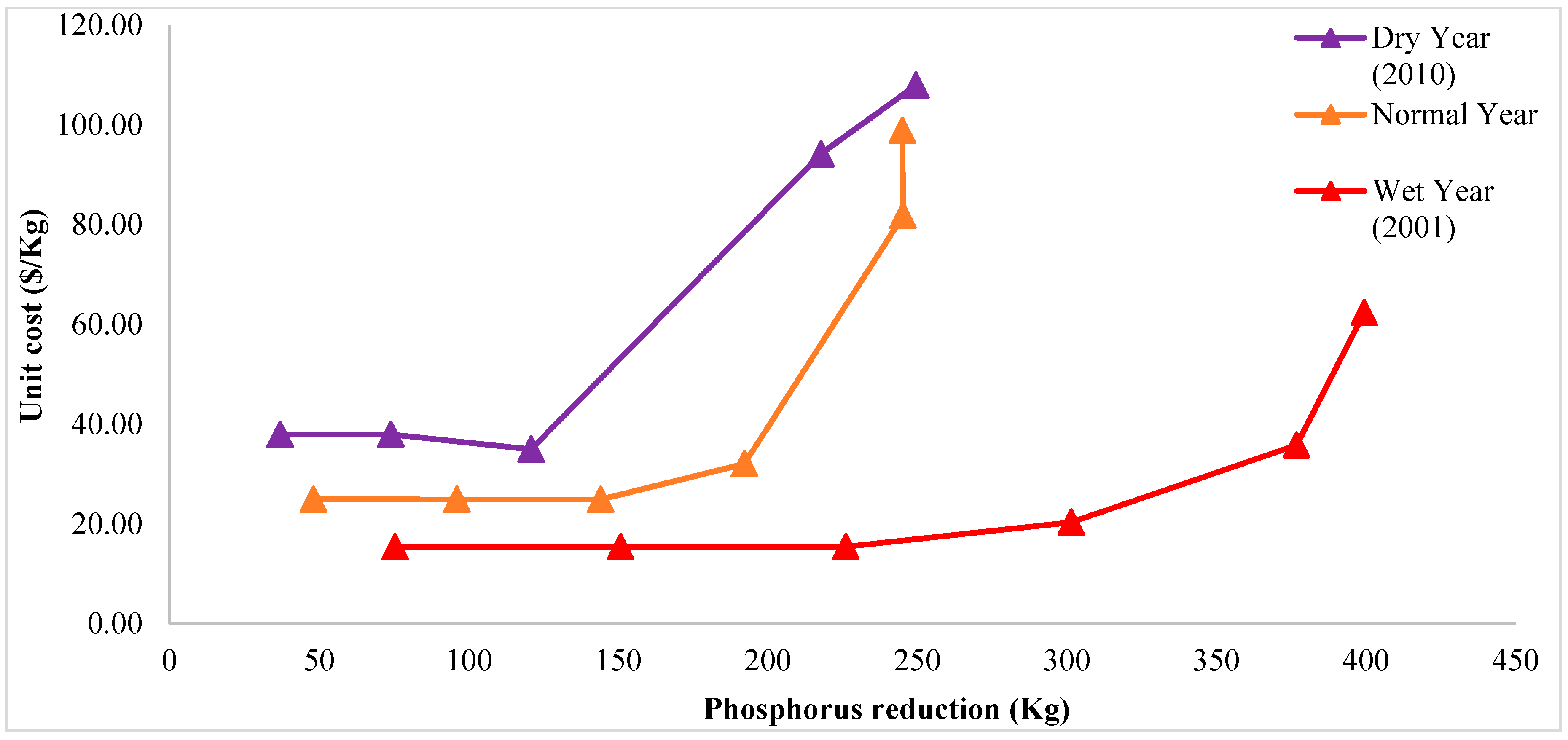
In the dry weather scenario (Table 6), at the lower level of the phosphorus reduction goal, nutrient management came out to be an effective BMP. At a 30% level of phosphorus reduction, nutrient management and ag land retirement were the two BMPs chosen. Note that in wet and normal scenarios, the only BMP selected to reduce this level of phosphorus was nutrient management. The cost to reduce 30% of the phosphorus from the baseline scenario was US$4226 in a scenario where dry weather prevailed. At this situation, nitrogen and phosphorus reduction costs per kg were US$22.54 and US$34.97, respectively. The maximum amount of phosphorus load reduction if dry weather prevailed was 41%, which costs US$169.58/kg for nitrogen and US$107.97/ kg for phosphorus. The relationship between phosphorus reduction per unit cost for all the three conditions, viz., normal, wet, and dry, are plotted in Figure 3. It is clear that phosphorus reduction cost per kg is the highest in a dry weather scenario and lowest in the wet weather scenario for all levels of phosphorus reduction.

The cost of controlling nitrogen, phosphorus, and sediment varies, among other things, based on the physical characteristics of soil, precipitation, BMPs used, and crops grown. Therefore, a kg to kg comparison across different regions or even different watersheds is not meaningful. Having said that, Gitau et al. (2004) [28] found the cost to be a dollar to reduce 0.6 kg of phosphorus. In a study conducted in Indiana, Maringanti et al. (2011) [29] indicated a per hectare cost of US$25–275 to reduce 37–76% phosphorus from the base level. The base level (without the implementation of any BMP) phosphorus release was 4 kg/ha. Liu et al. (2019) [30] studied combinations of best management practices to reduce total phosphorus in the agricultural-based AXL watershed in Indiana. They found the cost to control total phosphorus using a different combination of best management practices to be US$22-$139. Another study by Xu et al. (2018) [31] in a Lake Erie Watershed indicated the cost to reduce total phosphorus at the rate of US$0.10–$224 per hectare of land to reduce 46% of phosphorus from the base level.

7. Conclusions

Nonpoint source water pollution has been identified as one of the main contributors to water pollution in the United States. Our study showed that focusing on agricultural BMPs can reduce water pollution in rural watersheds such as the Saline Bayou Watershed studied here. We used biophysical simulation model (MapShed) and an economic optimization model to identify the minimum cost solution to meet alternative levels of phosphorus reduction. It was generally costly to reduce phosphorus in dry years compared to normal and wet years. Although it was possible to reduce more phosphorus in a scenario with wet weather, the per unit cost of reducing phosphorus in the watershed increased from US$15 per kg to US$62 per kg as the desired percentage of phosphorus reduction went up. In a normal weather scenario, the cost ranged from US$25 per kg at a low level of phosphorus reduction (48 kg of phosphorus reduction) to US$82 (245 kg of phosphorus reduction). The USDA NRCS can use the information derived from this study to tailor their incentive structure for each county in the United States. This analysis not only helps to set the realistic goal of reducing these pollutants but also to identify the most cost effective combination of BMPs to achieve the goal.

References

- Committee on Environment and Natural Resources (CENR). Scientific Assessment of Hypoxia in U.S. Coastal Waters; Interagency Working Group on Harmful Algal Blooms, Hypoxia, and Human Health of the Joint Subcommittee on Ocean Science and Technology; Committee on Environment and Natural Resources (CENR): Washington, DC, USA, 2010. [Google Scholar]
- Hypoxia Task Force (HTF). Gulf Hypoxia Action Plan 2008 for Reducing Mitigating, and Controlling Hypoxia in the Northern Gulf of Mexico and Improving Water Quality in the Mississippi River Basin; Environmental Protection Agency, Office of Wetlands, Oceans, and Watersheds: Washington, DC, USA, 2008.
- Paudel, K.P.; Gauthier, W.M.; Westra, J.V.; Hall, L.M. Factors influencing and steps leading to the adoption of best management practices by Louisiana dairy farmers. J. Agric. Appl. Econ. 2008, 40, 203–222. [Google Scholar] [CrossRef]
- US EPA. Waters Assessed as Impaired due to Nutrient-Related Causes. 2019. Available online: https://www.epa.gov/nutrient-policy-data/waters-assessed-impaired-due-nutrient-related-causes#rivers (accessed on 1 August 2019).
- US EPA. Office of Water and Office of Research and Development; National Rivers and Streams Assessment 2008–2009: A Collaborative Survey (EPA/841/R-16/007); US EPA: Washington, DC, USA, 2016. Available online: http://www.epa.gov/national-aquatic-resource-surveys/nrsa (accessed on 10 August 2019).
- Carpenter, S.R.; Caraco, N.F.; Correll, D.L.; Howarth, R.W.; Sharpley, A.N.; Smith, V.H. Nonpoint pollution of surface waters with phosphorus and nitrogen. Ecol. Appl. 1998, 8, 559–568. [Google Scholar] [CrossRef]
- US EPA. National Management Measures to Control Nonpoint Source Pollution from Agriculture. 2003. Available online: https://www.epa.gov/nps/national-management-measures-control-nonpoint-source-pollution-agriculture (accessed on 1 June 2019).
- Ribaudo, M.O.; Heimlich, R.; Peters, M. Nitrogen sources and Gulf hypoxia: Potential for environmental credit trading. Ecol. Econ. 2005, 52, 159–168. [Google Scholar] [CrossRef]
- Niraula, R.; Kalin, L.; Srivastava, P.; Anderson, C.J. Identifying critical source areas of nonpoint source pollution with SWAT and GWLF. Ecol. Model. 2013, 268, 123–133. [Google Scholar] [CrossRef]
- Tim, U.S.; Mostaghimi, S.; Shanholtz, V.O. Identification of critical nonpoint pollution source areas using geographic information systems and water quality modeling. JAWRA J. Am. Water Res. Assoc. 1992, 28, 877–887. [Google Scholar] [CrossRef]
- Sharpley, A.N.; Kleinman, P.J.A.; McDowell, R.W.; Gitau, M.; Bryant, R.B. Modeling phosphorus transport in agricultural watersheds: Processes and possibilities. J. Soil Water Conserv. 2002, 57, 425–439. [Google Scholar]
- Arnold, J.G.; Srinivasan, R.; Muttiah, R.S.; Williams, J.R. Large Area Hydrologic Modeling and Assessment Part I: Model Development1; Wiley Online Library: Hoboken, NJ, USA, 1998. [Google Scholar]
- Evans, B.M.; Lehning, D.W.; Corradini, K.J.; Peterson, G.W.; Nizeyimana, E.; Hamlett, J.M.; Robillard, P.D.; Day, R.L. A Comprehensive GIS-based modelling approach for predicting nutrient loads in watersheds. J. Spat. Hydrol. 2002, 2, 1–18. [Google Scholar]
- Ouyang, W.; Hao, F.-H.; Wang, X. Regional nonpoint source organic pollution modeling and critical area identification for watershed best environmental management. Water Air Soil Pollut. 2008, 187, 251–261. [Google Scholar] [CrossRef]
- Tripathi, M.P.; Panda, R.K.; Raghuwanshi, N.S. Development of effective management plan for critical subwatersheds using SWAT model. Hydrol. Process. 2005, 19, 809–826. [Google Scholar] [CrossRef]
- Ghebremichael, L.T.; Watzin, M.T.; Veith, T.L. SWAT modeling of critical source areas of runoff and phosphorus loss: Lake Champlain Basin, VT. In Proceedings of the 2009 International SWAT Conference, Texas Water Resources Institute Technical Report No. 356, College Station, TX, USA, 4–7 July 2009; pp. 385–393. [Google Scholar]
- Niraula, R.; Norman, L.M.; Meixner, T.; Callegary, J.B. Multi-gauge calibration for modeling the semi-arid Santa Cruz Watershed in Arizona-Mexico border area using SWAT. Air Soil Water Res. 2012, 5, 41. [Google Scholar] [CrossRef]
- Panagopoulos, Y.; Makropoulos, C.; Baltas, E.; Mimikou, M. SWAT parameterization for the identification of critical diffuse pollution source areas under data limitations. Ecol. Model. 2011, 222, 3500–3512. [Google Scholar] [CrossRef]
- Shang, X.; Wang, X.; Zhang, D.; Chen, W.; Chen, X.; Kong, H. An improved SWAT-based computational framework for identifying critical source areas for agricultural pollution at the lake basin scale. Ecol. Model. 2012, 226, 1–10. [Google Scholar] [CrossRef]
- White, M.J.; Storm, D.E.; Busteed, P.R.; Stoodley, S.H.; Phillips, S.J. Evaluating nonpoint source critical source area contributions at the watershed scale. J. Environ. Qual. 2009, 38, 1654–1663. [Google Scholar] [CrossRef] [PubMed]
- Jha, M.K.; Gassman, P.W.; Arnold, J.G. Water quality modeling for the Raccoon River watershed using SWAT. Trans. ASABE 2007, 50, 479–493. [Google Scholar] [CrossRef]
- Srivastava, P.; McNair, J.N.; Johnson, T.E. Comparison of process-based and artificial neural network approaches for streamflow modeling in an agricultural watershed. JAWRA J. Am. Water Res. Assoc. 2006, 42, 545–563. [Google Scholar] [CrossRef]
- Kirsch, K.; Kirsch, A.; Arnold, J.G. Predicting sediment and phosphorus loads in the Rock River basin using SWAT. Trans. ASAE 2002, 45, 1757–1769. [Google Scholar] [CrossRef]
- Spruill, C.A.; Workman, S.R.; Taraba, J.L. Simulation of daily and monthly stream discharge from small watersheds using the SWAT model. Trans. ASAE 2000, 43, 1431–1439. [Google Scholar] [CrossRef]
- Soil Conservation Service. National engineering handbook. Section 4- Hydrology; United States Department of Agriculture: Washington, DC, USA, 1985.
- Soil Conservation Service. Hydrology Training Series: Module 104—Runoff Curve Number Computations Study Guide; United States Department of Agriculture: Washington, DC, USA, 1989. Available online: https://www.wcc.nrcs.usda.gov/ftpref/wntsc/H&H/training/runoff-curve-numbers1.pdf (accessed on 10 August 2019).
- Moriasi, D.N.; Arnold, J.G.; Van Liew, M.W.; Bingner, R.L.; Harmel, R.D.; Veith, T.L. Model evaluation guidelines for systematic quantification of accuracy in watershed simulations. Trans. ASABE 2007, 50, 885–900. [Google Scholar] [CrossRef]
- Gitau, M.W.; Veith, T.L.; Gburek, W.J. Farm-level optimization of BMP placement for cost-effective pollution reduction. Trans. ASAE 2004, 47, 1923–1931. [Google Scholar] [CrossRef]
- Maringanti, C.; Chaubey, I.; Arabi, M.; Engel, B. Application of a multi-objective optimization method to provide least cost alternatives for NPS pollution control. Environ. Manag. 2011, 48, 448–461. [Google Scholar] [CrossRef]
- Liu, Y.; Wang, R.; Guo, T.; Engel, B.A.; Flanagan, D.C.; Lee, J.G.; Li, S.; Pijanowski, B.C.; Collingsworth, P.D.; Wallace, C.W.; et al. Evaluating Efficiencies and Cost-effectiveness of Best Management Practices in Improving Agricultural Water Quality Using Integrated SWAT and Cost Evaluation Tool. J. Hydrol. 2019, 123965. [Google Scholar] [CrossRef]
- Xu, H.; Brown, D.G.; Moore, M.R.; Currie, W.S. Optimizing spatial land management to balance water quality and economic returns in a Lake Erie watershed. Ecol. Econ. 2018, 145, 104–114. [Google Scholar] [CrossRef]
Figure 1.
Location of the Saline Bayou Watershed, Louisiana, USA.
Figure 2.
Calibration and Validation of Saline Bayou Watershed. Calibration statistics: NSE = 70%, PBIAS = 0.00, RMS = 0.55, and R2 = 0.70. Validation statistics: NSE = 59%, PBIAS 198 = 0.21, RMS = 0.64, and R2 = 0.64). NSE: Nash–Sutcliffe Efficiency; PBIAS: percent bias; RMS: ratio of root mean square error; R2: Coefficient of Determination. Dates are presented in the (month/ day/year) format.
Figure 3.
Per unit cost of phosphorus reduction using different best management practices in the Saline Bayou Watershed.