Validation of the 3D-MOHID Hydrodynamic Model for the Tagus Coastal Area
by
 , ,
, ,
Hilda de Pablo
1,*, 
João Sobrinho
1,
Mariangel Garcia
1,
Francisco Campuzano
1,
Manuela Juliano
2 and
Ramiro Neves
1 1
Marine Environment & Technology Center-MARETEC, Instituto Superior Técnico, University of Lisbon, Av. Rovisco Pais 1, 1049-001 Lisbon, Portugal
2
Marine Environment and Technology Laboratory-LAMTec-ID, University of Azores, Av. Álvaro Martins Homem Marina, Praia da Vitória Santa Cruz, 9760-412 Azores, Portugal
*
Author to whom correspondence should be addressed.
Water 2019, 11(8), 1713; https://doi.org/10.3390/w11081713
Submission received: 13 July 2019
/
Revised: 13 August 2019
/
Accepted: 14 August 2019
/
Published: 17 August 2019
(This article belongs to the Section Hydrology)
Abstract
:The hydrodynamics of the TagusROFI (Regions of Freshwater Influence) is affected by the coastal upwelling, the estuarine tidal flow, the thermohaline circulation that is modulated by the Tagus freshwater discharge, and by its complex bathymetry. The use of numerical models is the best way to explain the processes that characterize this region. These models are also crucial to answer important scientific and management questions. Nevertheless, the robustness of the products derived from models depend on their accuracy and therefore models must be validated to determine the uncertainty associated. Time and space variability of the driving forces and of bathymetry enhance flow complexity increasing validation difficulties, requiring continuous high-resolution data to describe flow and thermohaline horizontal and vertical variabilities. In the present work, to increase the precision and accuracy of the coastal processes simulations, the sub-systems coastal area and the Tagus estuary were integrated into a single domain, which considers higher resolution grids in both horizontal and vertical directions. The three-dimensiosal (3D)-MOHID Water model was validated for the TagusROFI by comparing statistically modelling results with in situ and satellite L4 data. Validation with a conductivity, temperature, and depth probe (CTD), an acoustic doppler current profiler (ADCP) and satellite data was performed for the first time. Validation against tidal gauges showed that the model is able to simulate tidal propagation inside the estuary with accuracy. A very good agreement between CTD data and surface sea water temperature (SST) and salinity simulations was observed. The validation of current direction and velocity from ADCP data also indicated a high model accuracy for these variables. Comparisons between model and satellite for SST also showed that the model produces realistic SSTs and upwelling events. Overall results showed that MOHID setup and parametrisations are well implemented for the TagusROFI domain. These results are even more important when a 3D model is used in simulations due to its complexity once it considers both horizontal and vertical discretization allowing a better representation of the heat and salinity fluxes in the water column. Moreover, the results achieved indicates that 3D-MOHID is robust enough to run in operational mode, including its forecast ability, fundamental to be used as a management tool.
1. Introduction
Modelling coastal systems particularly in regions of freshwater influence (ROFI), as it is the case of the Tagus estuary and its coastal adjacent area, is paramount to understand the physical and biogeochemical processes that characterize them. The simple measurement of environmental variables in situ alone or time-limited studies is not sufficient to translate and fully comprehended coastal processes since coastal systems are complex, decomposable, and large-scale [1]. Indeed, the combination and interaction of the physical factors (bathymetry; coastline topography; estuarine outflow; heat flux through the sea surface) and the associated physical transport and dispersal processes of the coastal flow field, makes coastal systems complex and unique in its hydrodynamics [2,3]. Therefore, and like other large-scale systems, the coastal system must be partitioned or decomposed into a number of small systems and the best way to gain insights into coastal system structure, organization, and functioning is through the use of numerical models. These models, besides allowing a better understanding of the interactions between the various components of the system, are also indispensable to set scientific scenarios and to answer important scientific and management questions [4]. Thus, only the proper knowledge of the processes that characterize the coastal systems, and their evolution in space and time, allow the design of robust coastal management plans. In this regard, hydrodynamic models assume a preponderant role since the establishment of currents and density fields is fundamental for transport models, whether they are Eulerian or Lagrangian, due to the importance of advection and/or diffusion in the study of issues related to the coastal system.
Among the numerical models that have been used to simulate the hydrodynamics of coastal systems (e.g., MARS3D [5]; MIKE3 [6]; SELFE [7]; SHYFEM [8]; TELEMAC [9]; MIKE 21/3 [10]; CSIRO [11]; Delft3D [12]), MOHID Water (Portuguese acronym of MOdelação HIDrodinâmica) is one of the most widely used. The MOHID Water model was developed by MARETEC (Marine and Environmental Technology Research Center). MOHID Water is open-source and most relevant key strengths are its ability to: Deal with two-dimensional (2D) and 3D simulations, with sigma, cartesian or lagrangian vertical coordinates; deal with eulerian or lagrangian transport references; use the same biogeochemical formulations independently of the number of spatial dimensions or space reference; and incorporate alternative formulations for every process (due to its modular approach). The versatility and flexibility of the MOHID Water eases its implementation in any type of system and to accomplish different modelling requirements depending on the objectives of the work to be performed. Indeed, in the last four years the MOHID Water was applied in multiple studies worldwide, namely in Canada [13], Colombia [14,15], Brazil [16], Argentina [17,18], Uruguay [19], Holland [20], France [21], Spain [22], Croatia [23], Australia [24,25], Malaysia [26] and Korea [27]. In Portugal, this model has been implemented in the entire Portuguese coast [28,29,30] and in all main estuaries [31,32,33,34,35].
Specifically, in the coastal system that comprises the Tagus estuary, most of the studies that used MOHID Water considered the coastal area and the Tagus estuary as sub-systems. In the case of the sub-system estuary, studies focused on sediment dynamics [36,37,38], on chlorophyll and/or nutrients [39,40], on microbiology [41,42], on water level [43], residence time [44] and CO2 fluxes [45]. Concerning the sub-system coastal area, studies were directed to analyse the effects of the Tagus estuarine plume [45,46,47].
All the above mentioned works regarded the sub-systems estuary and adjacent coastal area as different domains due to the spatial resolution that is required to represent local physical processes [48,49]. However, computational advances allowed to integrate both sub-systems into a single domain, which considers higher resolution grids in both horizontal and vertical directions, essential to increase the precision and accuracy of the coastal processes simulations [50]. For this reason, only recently those two sub-systems were considered and modelled as an estuarine-coastal continuum [47] using a variable grid in the horizontal axis, in order to have a higher horizontal resolution within the estuary and within the adjacent continental shelf.
In order to use model outputs, models should be scientifically sound and robust, and therefore must be validated to inform users how much confidence can be placed in the products. Model validation is a process that aims to demonstrate that a given site-specific model is capable of making sufficiently accurate simulations [51]. Nevertheless, despite the importance of the validation process and although several statistical indexes have been developed and used for model evaluation [51,52,53], there is a lack of a common validation procedure [53]. Notwithstanding, the robustness of the models must be demonstrated which is only possible by comparing the model simulated results with in situ or remote observations such as satellite or HF radar products. Although the MOHID model is periodically validated, none of the works published until now focus exclusively on the validation of the 3D-MOHID for the TagusROFI. Only Vaz et al. [47] validated the coastal area circulation model through the comparison of the superficial velocity predictions with HF Radar data for this domain in the vicinity of the estuary mouth for 2012. These authors found that model predictions do not fit perfectly with the HF radar data probably due to the high spatial variability of velocity that changes in spatial scales shorter than the model cell size. Nonetheless, in 3D hydrodynamic models, validation requires the comparison of the model results with at least sea level, current speed, and current direction [54,55], and since the model application is baroclinic, validation should also consider seawater temperature and salinity. Janeiro et al. [30] validated a 3D application of the MOHID Water model for southern Portugal by comparing in situ measurements and HF Radar with predictions for all the five variables above. Although the TagusROFI domain has been applied in several research studies and as a tool for its management, this study will provide a higher insight concerning the validation of the results.
The present study aims to validate a 3D baroclinic application of MOHID Water model for the TagusROFI domain by using the above variables from a spatial-temporal perspective. With this purpose, model results will be compared with in situ measurements from several types of sensors (tidal gauges, CTD, and ADCP) and satellite L4 products (OSTIA, ODYSSEA, and MUR). The present work uses CTD, ADCP and satellite data to validate the TagusROFI domain for the first time. The main results are discussed, and conclusions are drawn concerning the model implementation in representing the coastal physical processes, its robustness to run in operational mode, including its forecast capability and consequently its ability to be a useful and powerful tool for coastal environmental management.
2. Materials and Methods
2.1. Study Area
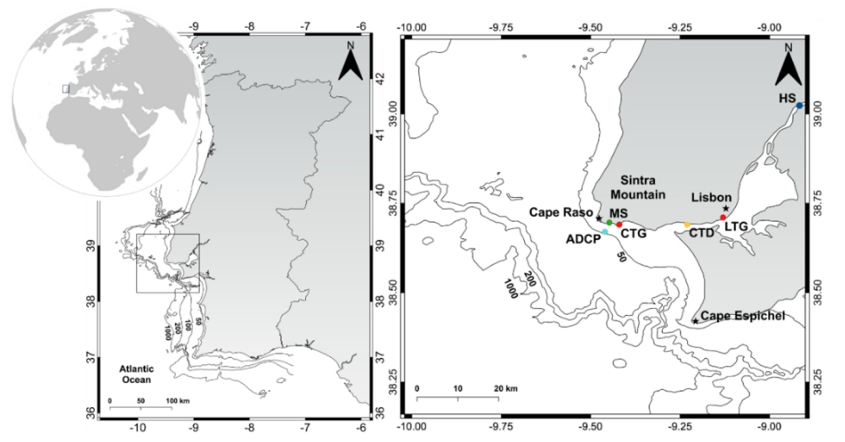
The study area is located in the Portuguese west coast (30.6° N–9.5° W) and comprises a ROFI zone (Region of Freshwater Influence) (Figure 1) that encompasses the Tagus estuary, which is a highly populated region, subject to both natural and human pressures. This is the most extensive estuary of the Iberian Peninsula that occupies a volume of 1.9 × 10⁹ m3 and a surface area of approximately 320 km2 [7,56]. This estuary is composed of a central body 30 km long and 10 km wide, connected to the Atlantic Ocean through a channel 12 km long and 2 km wide [57] forming a NE-SW oriented talweg [58]. Its width varies from 400 m at its head to 15 km in the central bay, with a depth range of 0 to 20 m (average depth of 5.1 m) [59], and presents extensive intertidal zones that occupy 40% of the estuary [60]. The coastal zone adjacent to the open ocean of the study area comprises 70 km of continental shelf that extends along the 39° N parallel, limited by the Cape Raso in the north and the Cape Espichel in the south, with the shelfbreak at 140 m depth [61]. It is a narrow platform that extends, on average, until 180 m depth and with a width ranging from 3 km (near the Cape Espichel) to 30 km [61]. This area is dominated by two important geomorphological features, the Cascais and Lisbon submarine canyons (the Cascais canyon is located NW of the Lisbon canyon and separated from the latter by the 1000 m high ridge of the Afonso Albuquerque Plateau [62]).
The Tagus estuary is a semi-diurnal mesotidal estuary, presenting an average amplitude of 2.4 m at the river mouth with the tidal range varying from 0.9 m to around 4.1 m during neap tides and spring tides, respectively [63]. According to Guerreiro et al. [7], river discharge may significantly influence water levels until 40 km upstream of the mouth, whereas downstream the levels are mainly controlled by tide and storm surges. The annual average river flow is 258 m3 s−1, with monthly averages ranging from 6 to 2090 m3 s−1 (2006–2018; National Water Resources Information System, SNIRH), and although being usually a well-mixed estuary, stratification may occur at high flow rates [64]. Flow is related to the amplitude of the tide which is also responsible for the mixture processes within the estuary. Indeed, the primary driver of the circulation in the Tagus estuary are tides, but other factors also influence it, such as river flow, atmospheric pressure, and the wind [65]. In addition, the estuary is strongly ebb-dominated due to the large extension of tidal flats [59].
In the adjacent area of the estuary, the configuration and orientation of the coastline protect the estuarine outflow from the waves, being only the southern part of the estuarine channel exposed to the swells [66]. Coastline geometry also influences plume dynamics, leading to a trajectory near the shore which is displaced offshore during northern winds events [46]. On the other hand, according to Jouanneau et al. [61], the continental shelf may also affect coastal currents, which in turn influences the mixture processes of the plume. Similarly, Fernández-Nóvoa et al. [58], stated that submarine canyons will modify the circulation on the shelf, whilst wind patterns in the ROFI are somehow controlled by the Sintra Mountains. In this area, predominant wind during winter is from northwest, north, and southeast (ranging from 1.5 m s−1, 8.5% of occurrence, to 14 m s−1, 7.5% of occurrence), whilst in summer winds from the north or from northwest prevail (ranging from 1 m s−1, 5% of occurrence, to 15 m s−1, 20% of occurrence) [47,67].
The general circulation on the western coast of the Iberian Peninsula presents a marked seasonal variability. Between May and September, the Portuguese west coast presents a generally equatorward flow (Portuguese Current; [68]) which is associated with the dominant regime of winds. During autumn and early winter, dominant winds are reversed becoming predominantly directed to E–N and a north poleward flow is observed (Portugal Coastal Counter Current; [69]). This current weakens when the northerly winds prevail developing conditions for the occurrence of seasonal upwelling (Portugal Coastal Current [70,71]), promoting an offshore advection of surface waters and vertical advection of rich nutrient upwelled waters toward the surface. To underline that the coastal area of the present study is characterized by significant and frequent upwelling events originated by jet-like flow extending more than 20 km seaward [72].
2.2. Model
The MOHID Water model assumes a hydrostatic equilibrium and Boussinesq approximation. To discretize the equations, it uses the finite volume approximation, so the discrete form of the equations that govern the flow can be applied macroscopically to the control volume (cell), permitting the equations to be independent of the cell geometry, allowing the use of a generic vertical coordinate [71]. According to Blazek [73], the main advantage of the finite-volume method over the finite-difference method is that the spatial discretization is carried out directly in the physical space, which avoids issues related to the transformation between the physical and the computational coordinate system. Moreover, the finite-volume method is very flexible and therefore can be easily implemented on both structured and unstructured grids [73].
The momentum balance equations for horizontal velocities are, in differential form and cartesian coordinates:
where, u, v and w are the components of the velocity vector in the x, y and z directions, f the Coriolis parameter, vH, and vv are the turbulent viscosities in the horizontal and vertical directions, p is the pressure. Assuming hydrostatic pressure the vertical momentum equation becomes an equation for pressure:
And vertical velocity is computed using the continuity equation (assuming constant density, according to the Boussinesq approach):
MOHID Water solves the seawater density using a non-linear state equation, depending on pressure, salinity and potential temperature using the algorithm of Millero and Poisson [74]. For the 3D momentum (zonal and meridional velocities), heat and salt balance equations in the vertical direction are computed implicitly while the horizontal directions are calculated explicitly for enhanced stability purposes [75].
The implementation of the study domain uses a one-way downscaling strategy of nested domains: the child high-resolution domain, TagusROFI, receives its open boundary conditions with 900 s temporal resolution from the lower resolution parent domain, the Portuguese Coast Operational Model System (PCOMS), which open boundary condition combines low-frequency Copernicus Marine Environment Monitoring Service (CMEMS) results (levels, salinity and temperature) with tidal levels computed by a 2D model with the same horizontal resolution (WestIberia domain). The downscaling strategy followed in this application was developed in the framework of the projects “European coastal-shelf sea operational observing and forecasting system” (ECOOP) and “Development and pre-operational validation of upgraded GMES Marine Core Services and capabilities” (MyOcean) and is subjacent to the CMEMS forecast modelling service rationale. This service provides large scale ocean forecasts of hydrodynamic and biogeochemical parameters which are refined locally by higher resolution models that can add the interaction with other forcing functions such as waves [9]. In our application, tide is the new forcing. The downscaling strategy using an intermediate regional model application between CMEMS and a local application has the advantage of running many local applications in parallel. In particular, PCOMS provides boundary conditions for all the major Portuguese estuaries such as the TagusROFI domain. In operational modelling this allows forecasts to be available in a smaller time period, as PCOMS can run separately from all its receiving child applications. Tide is imposed at the open boundary of the WestIberia domain using the version of the Finite Element Solution tide model (FES2004) global tide model [76,77]. Feedback into the parent domains is not considered. At the open boundary between nested domains, a Flather radiation method for the barotropic flow combined with a flow relaxation scheme to temperature, salinity, and total velocities was applied to the first 10 grid cells [78]. Turbulent diffusion coefficients are computed in MOHID using its embedded version of the General Ocean Turbulence Model (GOTM) [79].
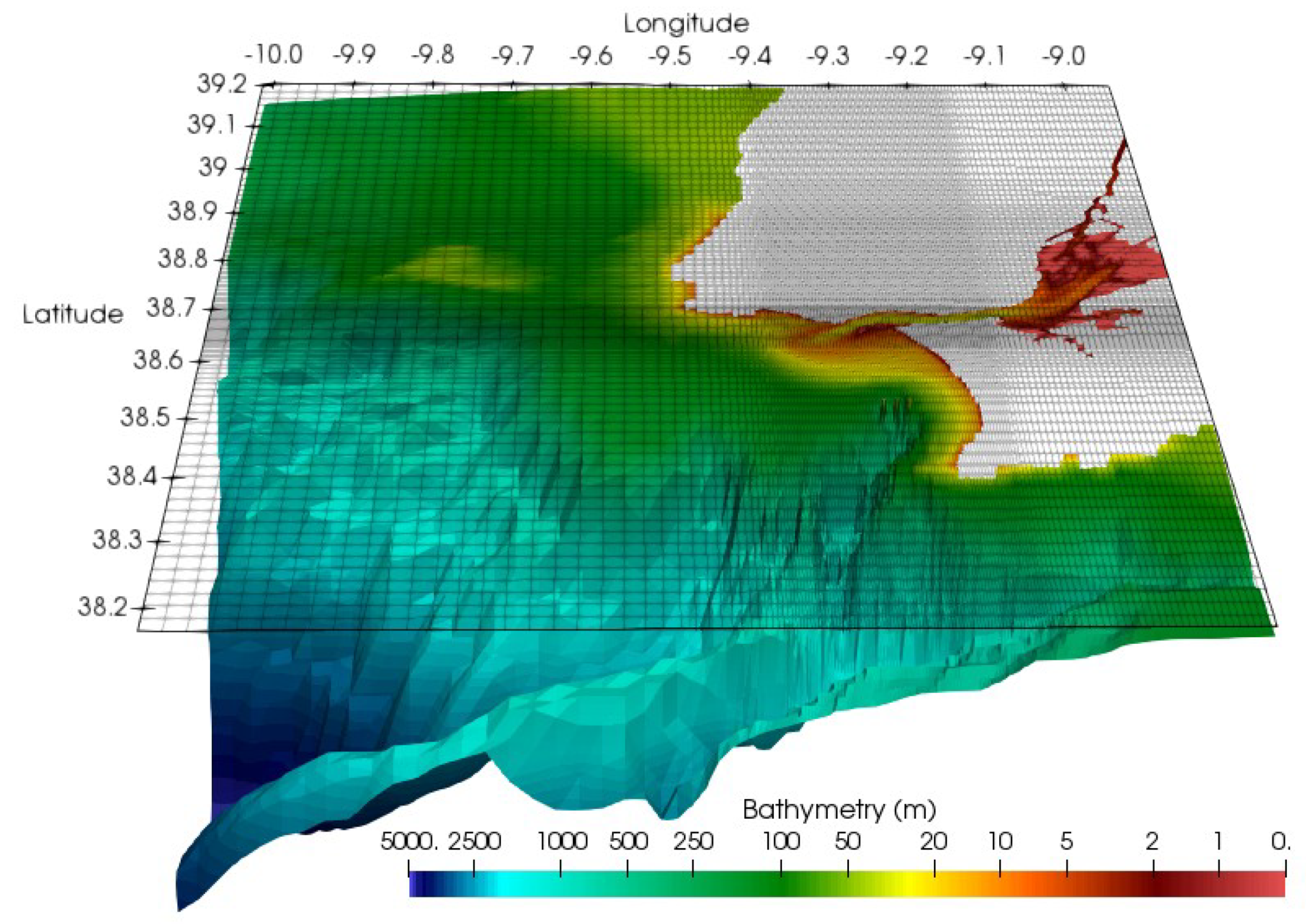
The PCOMS and the TagusROFI domains applications are a fully 3D baroclinic hydrodynamic and ecological model, capable of simulating a wide range of processes (e.g., hydrodynamics, transport, water quality, oil spills) in surface water bodies (oceans, coastal areas, estuaries, and reservoirs). The PCOMS domain covers the Continental Iberian Atlantic coast and its contiguous ocean. This domain presents a constant horizontal resolution of 0.06° (≈5.2 km) populated with bathymetric information derived from the EMODnet Hydrography portal and covers the area comprised by the latitudes 45.00° and 34.38° N and the longitudes 12.60° and 5.10° W, resulting in a grid of 177 × 125 cells and maximum depths around 5300 m. The TagusROFI domain presents a variable horizontal resolution (200 m–2 km), which is an area that covers the interior of the estuary and the coastal zone (coast W–E) resulting in a grid of 121 × 146 cells (Figure 2) comprised by the range of latitudes 39.21° to 38.16° N and of longitudes 10.02° to 8.90° W. In the present study, it was used the best bathymetric information currently available, which comes from bathymetric data collected by the Hydrographic Institute (IH) between 1964 and 2009 for the Tagus estuary, and from the General Bathymetric Chart of the Oceans (GEBCO) for adjacent coastal area. The bathymetry was generated through a Delaunay triangulation using both data sets which are very consistent in the overlapping area.
Both PCOMS and TagusROFI domains were forced in the surface by meteorological models which provide hourly fields of surface wind, temperature, relative humidity, pressure, and solar radiation. PCOMS is forced with MM5 (PSU/NCAR mesoscale model) meteorological model with 9 km of spatial resolution, while the TagusROFI domain was forced by the WRF (Weather Research & Forecasting) meteorological model with 3 km of spatial resolution [80].
Both domains share a common vertical discretization consisting on a mixed vertical geometry composed of a sigma domain with 7 layers from the surface until 8.68 m depth, with variable thickness decreasing up to 1 m at the surface, on top of a cartesian domain of 43 layers with thickness increasing towards the bottom [77]. Intertidal areas computation is subjected to land masks which take the value 0 (the model does not compute forces for that cell) when the water column is below 20 cm. For the bottom friction, a rugosity of 0.0025 m2 s−1 was used.
River discharges in the TagusROFI application were imposed as volume discharges (without momentum). The Tagus river discharge using the Almourol hydrological station (39.22° N, 8.67° W) data, located 70 km off the head of the estuary, and obtained from the National Water Resources Information System (SNIRH) service with a frequency of 1 h. Other minor rivers (Trancão and Sorraia) were imposed using climatological values, with river flow ranging between 3 and 60 m3 s−1 for Sorraia river and between 1 and 9 m3 s−1 for Trancão river. Monthly climatological values of freshwater temperature and salinity for the three rivers and for water discharges from 14 wastewater treatment plants (WWTPs) were also imposed. Model configurations for the TagusROFI are summarized in Table 1.
The actual implementation has been running operationally without interruption since 2011 providing a 3-day forecast once per day, for water velocity, water level, surface seawater temperature, salinity, and biogeochemical properties from a nutrient-phytoplankton-zooplankton- detritus (NPZD) model. The daily operational cycle consists of a 5-day simulation, starting the day before, in order to get the latest meteorological modelling results. Discharges are also updated every day with field data provided by the Almourol station thus providing the best flow value available. Forecasts are simulated using the last available river flow. The Level 3 configuration takes approximately 1 h and 30 min for each day of simulation under the configuration presented in Table 1.
2.3. Available Observations Data
Modelling performance was assessed through comparison with observations. All in-situ data and remote observations have advantages and disadvantages: The main advantage of tide gauges is that continuously record the height of the surrounding water level with a fine resolution, whereas the main disadvantage is its coarse spatial resolution in complex coastal areas. Similarly, the main advantage of CTD (salinity, temperature and depth data) is the frequency of data acquisition, whilst its disadvantage is the lack of spatial information. The ADCP (current velocity data) has the same advantages and disadvantages of a CTD but has as additional advantage the obtention of depth profiles along the entire water column. Satellite images has the advantage of providing daily surface maps (2D) of a region, but with very low frequency. This could be an issue for an area such as the TagusROFI that is dominated by small temporal scales. The data sets used for this purpose were the following:
2.3.1. Water Level
The water level was obtained from two tidal gauges, one located within the Tagus estuary (Lisbon harbor-LTG; 38.71° N and –9.13° W) and the other placed in the adjacent coastal area (Cascais-CTG; 38.69° N and −9.42° W) (Figure 1). Data from LTG was provided by the Hydrographic Institute, whereas data from CTG is available from the General-Directorate of the Territory web site. Distance between these tidal gauges was approximately 25 km (in a straight line). Modelling results were compared with data obtained in October 2012 from both tidal gauges with a time interval of regular 10-minute, comprising one spring and one neap tide.
2.3.2. Seawater Temperature and Salinity
Surface seawater temperature (SST) and salinity were recorded at 1 m depth every 10 min using a CTD (YSI 6600 V2) placed at the entrance channel of the Tagus estuary (38.69° N and –9.23° W) (Figure 1). Both variables were compared with the results obtained from MOHID, in the period between November 2012 and April 2013.
2.3.3. Current Velocity
Current velocity was registered using an ADCP (Teledyne Marine WorkHorse Sentinel, 600 kHz, WHS600 with four beams) placed at surface, off Cascais (38.67° N and –9.46° W) (Figure 1). This equipment recorded eastward and northward current, at 15 min sampling intervals, during the period from 2 to 17 July 2009.
The velocity vector was measured along the entire water column, every 1 m. In the present study, after analysing the profile of the current velocity, the water column was split into two layers from 2.5 and 15 m and from 15 to 30 m. In the top layer, current velocity is higher and dominated by the action of the wind, whilst in the bottom layer the effect of wind very reduced. For each layer, the mean value was obtained for the eastward and northward components as well as for the intensity. Modelling results were interpolated using the ADCP grid disregarding data obtained in the first 2.5 m and in the last 5 m water depth, to avoid bias due to the Doppler noise.
2.3.4. Seawater Temperature Based on Satellite Images
In order to compare the results obtained from MOHID with satellite images, three level 4 gridded RS data products were used, namely, OSTIA ([84], https://doi.org/10.5067/GHOST-4FK01), ODYSSEA (http://marine.copernicus.eu/; [85]), and MUR (http://doi.org/10.5067/GHGMR-4FJ01).
These products have a spatial resolution of 5, 2 and 1 km, respectively. Level 4 products are more accurate than other products since they combine complementary information from several satellite sensors and in situ instruments, being generated through statistical interpolation and temporal averaging [86]. According to Parkinson et al. [87], these products have also the advantage of providing gap-free gridded outputs. Each of these products, establish a reference depth used to correct bias and to integrate data into a single product. Daily SST satellite images were compared with the daily average of SST derived from the model (hourly outputs). The comparisons were performed for the period 2014–2016 and the statistical metrics correspond to the annual average obtained from the daily averages of SST.
2.4. Statistics
Various statistical indexes exist to evaluate the quality of the model’s calibration and validation results. Nonetheless, there is a lack of standard validation procedure. In the present study, observed and modelled results were compared using the correlation coefficient (r), root mean square error (RMSE), and BIAS index (mean error). The formulas that express these statistics followed the ones presented in Williams and Esteves [55] where n represents the number of model/observation data pairs, whilst M and O stand for model and observation, respectively:
The correlation coefficient (also referred as Pearson product-moment correlation) measures the strength and direction of the relationship between two variables and can be either positive or negative depending on the directionality of the estimate. The correlation coefficient ranges from −1 to 1. A value of 1 indicates that the linear equation describes the relationship between M and O perfectly, whereas a value of 0 indicates that there is no linear correlation between the variables. Negative values indicate that M decreases as O increases.
The model bias is a simple statistic, which measures the mean deviation between model-predicted values (M) and the observation data (O) and can be either positive or negative reflecting an over- or underestimation of observations by the model, respectively. Similar to RMSE, the smaller the absolute values of bias the better the agreement between model-predicted values and observation data.
The RMSE is a generalized form of standard deviation that measures the deviation between model and observations in a least-squares sense. The square of the deviations ensures that negative as well as positive contributions are added, whereas the square-root restores the units to that of the original variable. RMSE has the benefit of penalizing large errors. Small absolute values of RMSE indicates a good agreement between model and observations.
3. Results and Discussion
3.1. Water Level–Time Series Data
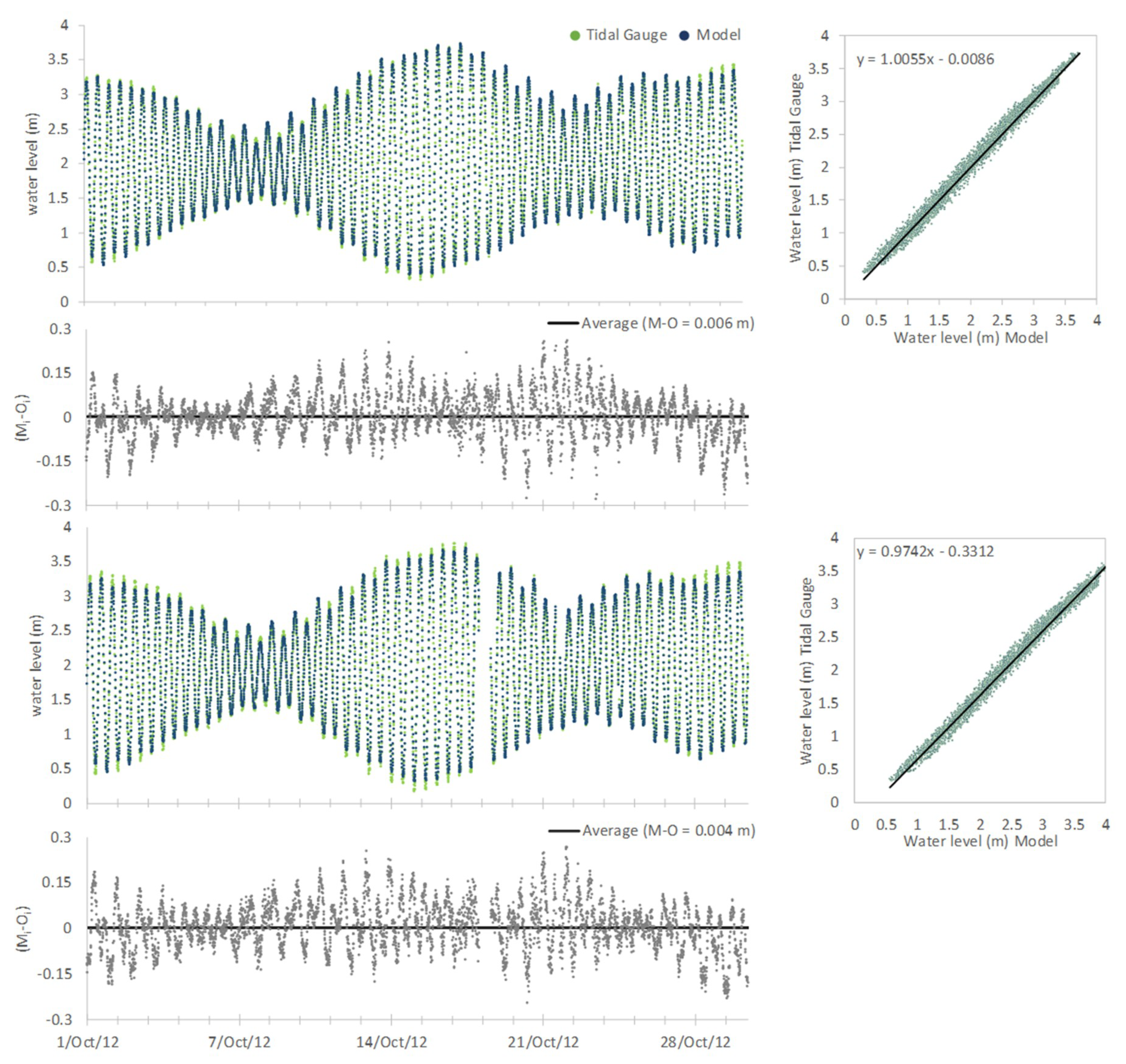
Figure 3 shows the comparison between the results of the model with the data obtained for water level through the tide gauges for Cascais (CTG) and Lisbon (LTG) stations. The comparison interval refers to a full month (October 2012) covering one ebb and one flood tide period. The mean difference between modelling results and observations for CTG varied between −0.28 m and 0.26 m with an average of 0.003 m, whereas for LTG ranged from −0.24 m to 0.27 m with a mean average of 0.004 m (Figure 3). In both stations, the higher differences were registered during slack water. During these periods, the effect of the tide is less pronounced and thus the effect of wind on water level is evident. Model results showed an excellent agreement with the data measured in amplitude and tidal phase for both stations (CTG and LTG), reproducing accurately the measurements obtained in situ and for all periods of the tide. This is corroborated by the results of the statistics that were performed to evaluate the coherence between simulated and observed data for water level (Figure 3; Table 2).
A strong correlation was observed for both stations between modelling results and observed data (CTG: r = 0.995; LTG: r = 0.994) which is in concordance with the RMSE error determined for both stations (Table 2). The BIAS determined was close to zero indicating that modelling results and observed values do not differ significantly. Altogether, these results highlight the capacity of the MOHID Water model to simulate the tidal propagation in a highly dynamic estuary mouth.
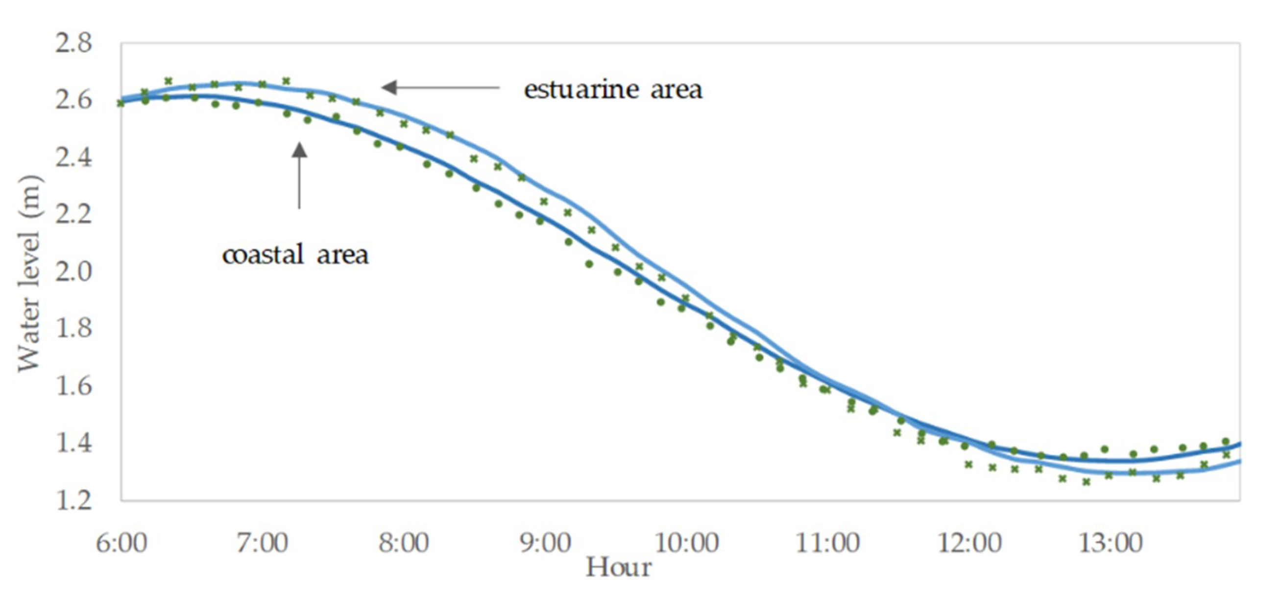
The tidal wave is amplified when it moves into the estuary as a consequence of the reduction of the depth which, along with the high velocities of the flow, causes the refraction of the tidal wave and consequently the increase of its amplitude. This phenomenon can be observed in Figure 4, which corresponds to a zoom of 7.5 h of Figure 3 that encompasses an ebb period. Data from CTG and LTG revealed a wave time-lag of approximately 20 min and an increase of the amplitude of about 15–20 cm between both stations. Both tidal wave time-lag and differences on the tidal wave amplitude between stations were well reproduced by the model (Figure 4).
3.2. Seawater Temperature and Salinity–Time Series Data
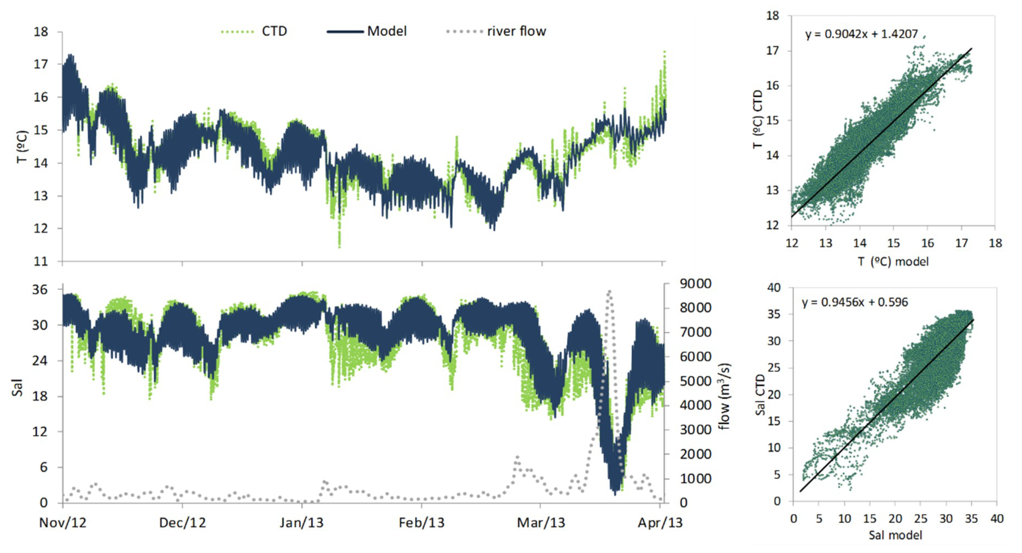
Between November 2012 and April 2013, seawater temperature and salinity were obtained at surface (1 m depth) with a CTD located in the area further downstream of the outlet channel of the estuary. These data were compared with a time series extracted from the model for the same local. During the study period, the average river flow was 522 m3 s−1, ranging from 44 to 8711 m3 s−1 (Figure 5). From the analyses of Figure 5, it can be seen that the observed and simulated results present a similar pattern for both variables. Daily fluctuations observed in SST and salinity were related to different river flows during flood and ebb periods. The high Pearson correlations coefficients obtained for SST (r = 0.91) and salinity (r = 0.86) reveal the good agreement between observations and simulated results (Figure 5; Table 3).
The low values obtained for RMSE error and BIAS (Table 3) indicates that modelling results and observed values for SST are in good agreement. Regarding salinity, although the BIAS obtained was extremely low reflecting an overall low difference between observed and simulated results, the RMSE error determined, despite being considered low, was higher than 2 (Table 3). Model results were obtained with the operational forecasting model in which the river flow is daily updated. However, sometimes it occurs that the flow is not updated on the database in due time and therefore the model uses the last data available. Whenever this happens, a time-lapse between the real river flow and the one used in simulations occur. Time lapses are not uncommon but usually do not exceed 3 days. This may constitute an issue if during this period the river flow is atypical which will affect negatively forecasting. Indeed, this was verified during the period under study which may explain the low value of RMSE determined.
Although the salinity within the estuary depends on the entrance of freshwater, the main driver that controls the mixing processes is the tide. Considering that the tidal prism inside the Tagus estuary is 640 × 106 m3, the river flow is only relevant to the non-linear mixing processes during high river flow events. At the end of the comparison period, an extreme event occurred where the mean daily river flow over three consecutive days attained 7500 m3 s−1 which represents 25% of the volume of the tidal prism. This has led to the abrupt decrease of salinity (Figure 5).
Data from CTD put in evidence this extreme event, registering very low salinity values outside the estuary’s mouth (Figure 5), indicating that MOHID is well implemented for the estuary regarding transport and mixing processes. Furthermore, also reveals that the boundary conditions obtained from the Portuguese Coastal Operational Modelling System are appropriate.
3.3. Currents–ADCP Analysis
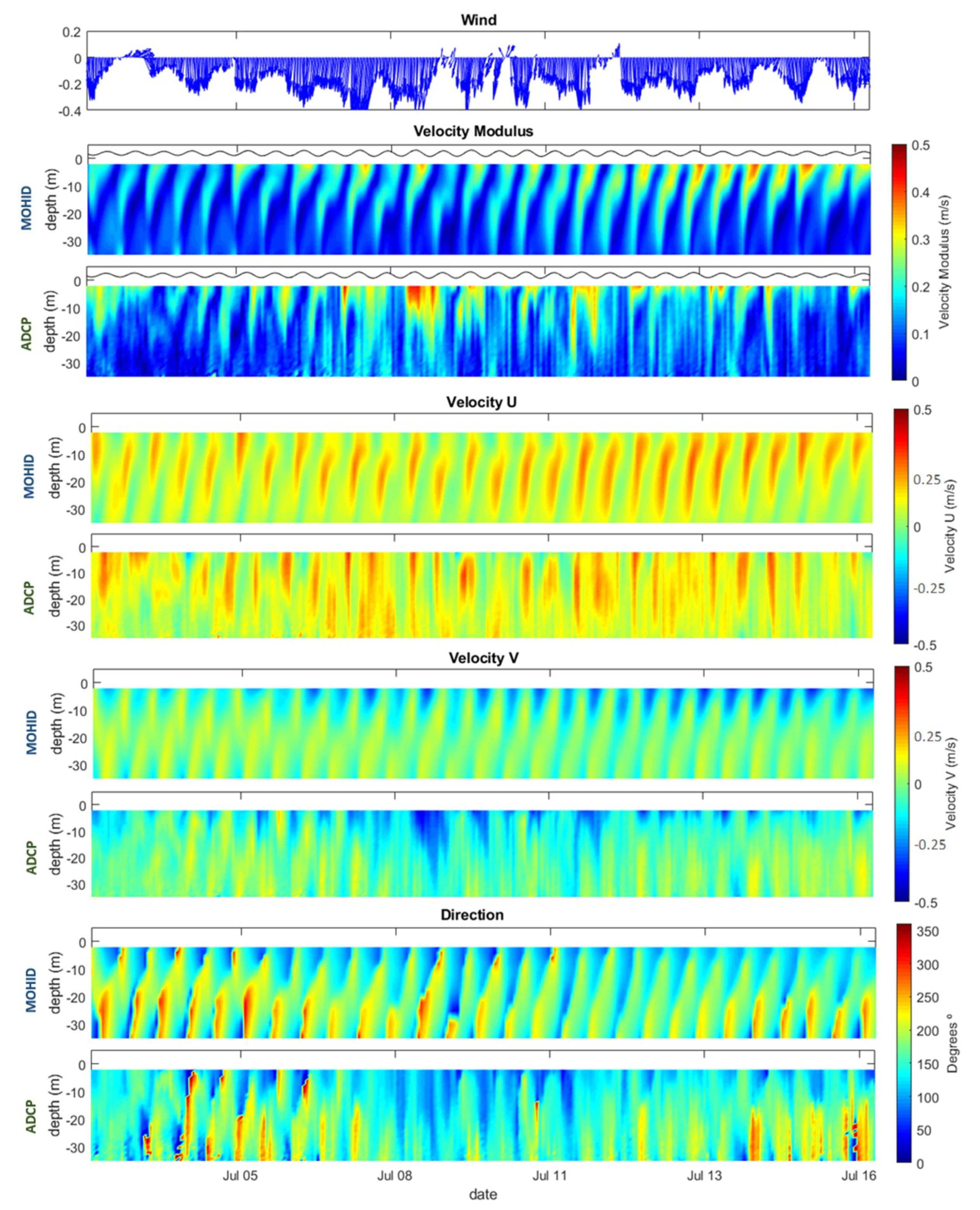
During the period of comparison, the prevailing wind was from the north quadrant with an average intensity of 3.4 m s−1 (ranging from 0.1 to 9.2 m s−1; data recorded in MS, Figure 1), and the mean flow rate of the river was 104 m3 s−1 (varying between 27 and 451 m3 s−1; data recorded in HS, Figure 1). Figure 6 compares raw data from ADCP with model results. There is a good qualitative agreement between the present model and ADCP measurements since predictions follow the same pattern of the observation data for current intensity and direction, as well as for both components of velocity (u and v). Periodical oscillations on the direction of the current due to tide are also perceptible in Figure 6.
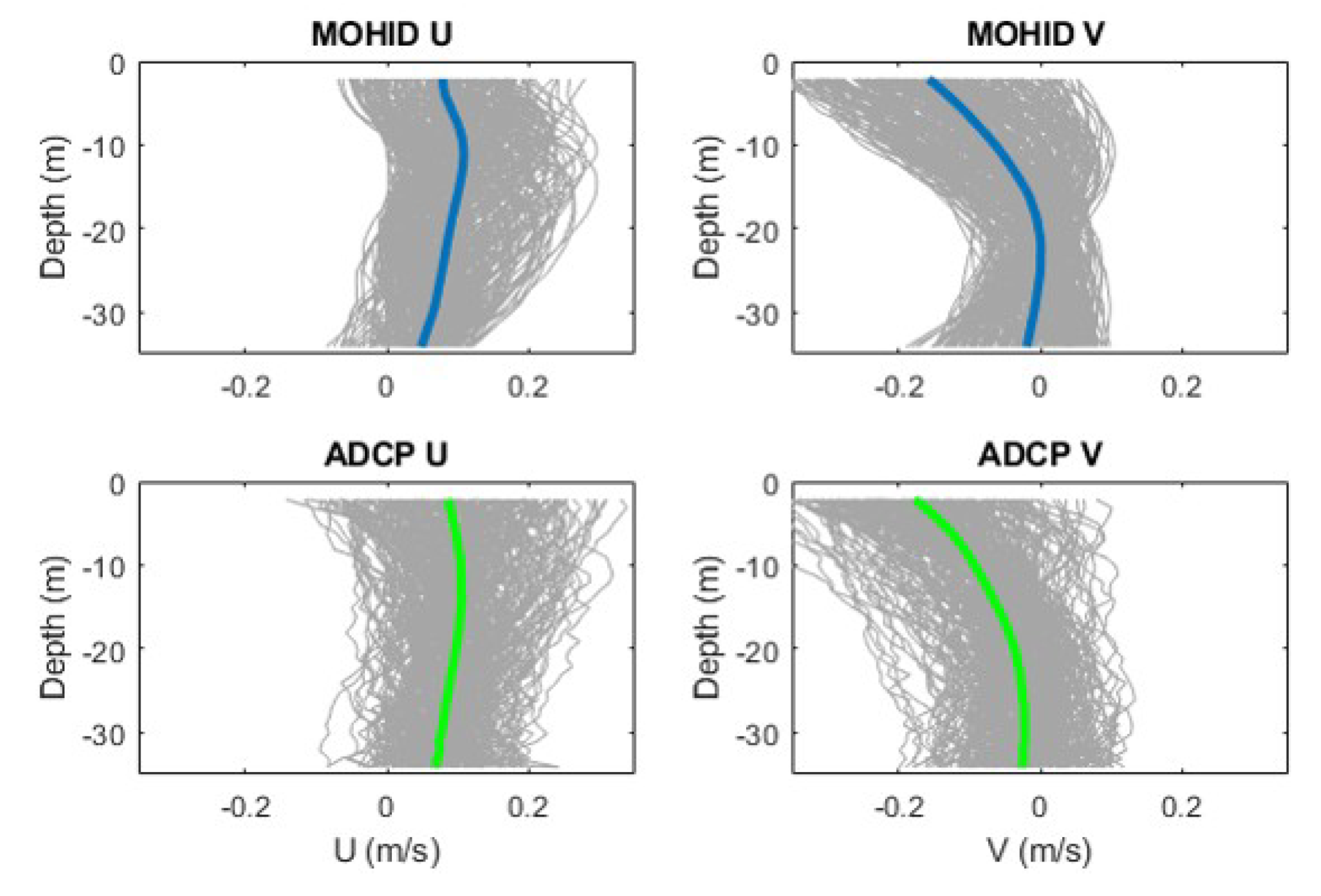
ADCP data were obtained in an area that is protected from the North winds by the Sintra Mountains and weakly influenced by the Tagus plume due to the morphological characteristics of the estuary that leads it southwest which in turn is forced to move north due to Coriolis force. Nevertheless, measurements and modelling results showed that higher superficial current velocities had a southern direction, mainly due to the prevailing north winds during the study period. North winds, and consequently upwelling conditions, intensifies the surface velocity´s v component and forces it to move southwards almost during the entire period. The distribution pattern of the current direction results fundamentally from the tide that confers a harmonic behaviour to the flow. There is a mismatch in the direction of the prevailing current between the surface and the bottom, due to the variation of current velocity with the increase of depth which makes the fluid inertia to be different. Indeed, surface layers are subject to a stronger wind stress than the middle and bottom layers, since the influence of the wind decreases as depth increases. Thus, the water surface usually presents higher current velocities, which are directly related to wind direction and intensity. This can also be observed in Figure 7, where velocity profiles at each moment are presented for both observations and modelling results. The model reflects with high accuracy the individual and mean profiles obtained through ADCP.
Since the influence of the wind on the water column is higher in the top meters, the statistical analysis was performed for two depth layers (between 2.5 m–15 m and 15 m–30 m) (Table 4). The coefficient of correlation was relatively high and varied between 0.63 and 0.73 and between 0.62 and 0.71 for the first and second water column layer, respectively. For both layers, the RMSE and BIAS obtained for velocity modulus, and for the current components of the velocity (u and v) was always lower than 0.2 which indicates a statistically significant fit [55]. Regarding the current direction, the RMSE and BIAS determined indicate the occurrence of slight differences between observed and simulated data. According to Williams and Esteves [55], the minimum-level model performance should be ±15° for BIAS which is in accordance with the results obtained.
The results obtained clearly shows the reproducibility of the model in representing the 3D water column in the coastal zone, where nonlinear processes (interaction between wind/ tides/ oceanic circulation/ bathymetry interaction) become more important. Since vertical stratification of the velocity was well captured by this MOHID Water application, it can be inferred that bottom rugosity and vertical diffusion are correctly implemented in the model.
3.4. Seawater Temperature–Validation with Satellite
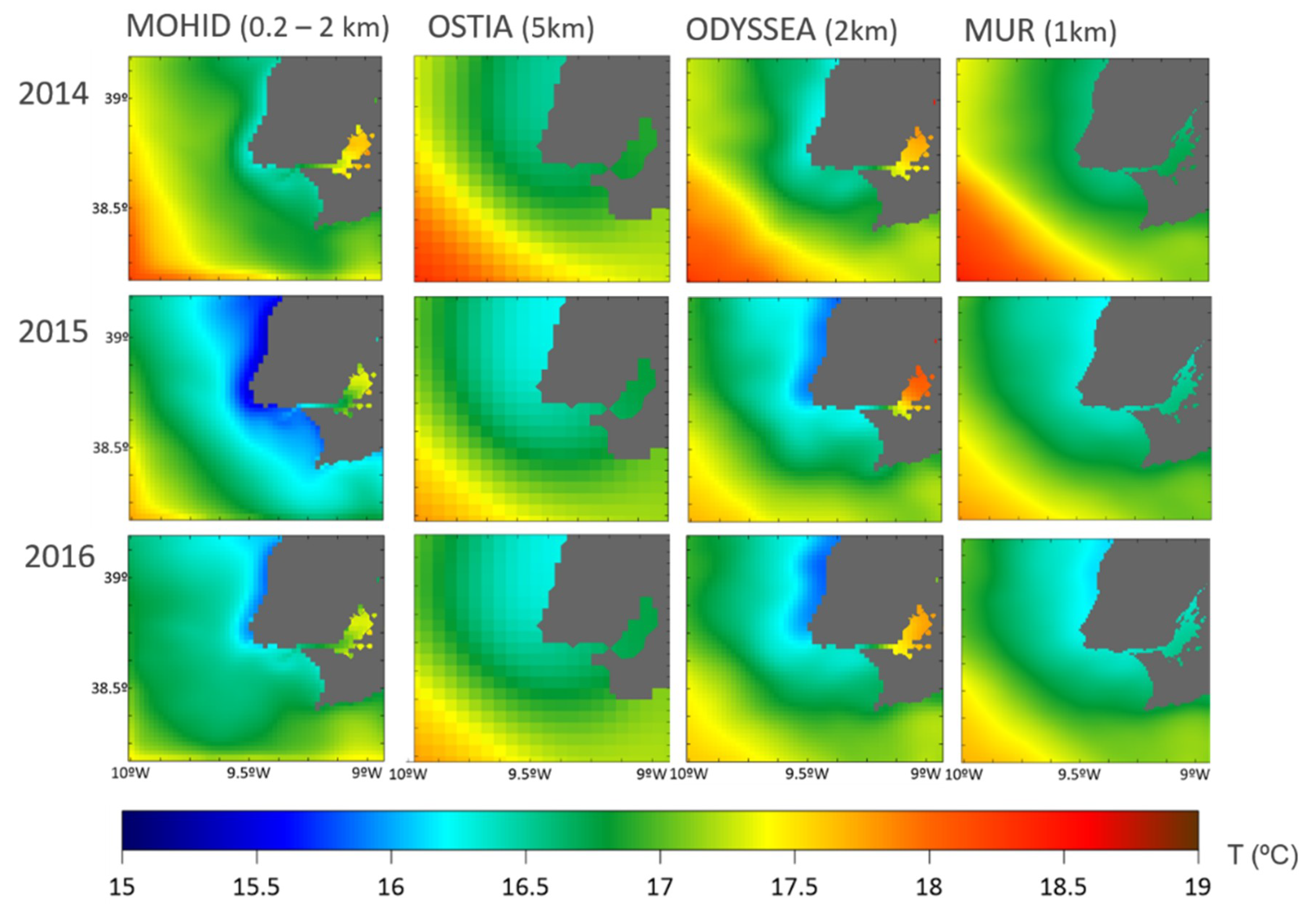
In the last decade, remote sensing data have been used to characterize coastal systems because they provide information on several variables with higher comprehensive spatial scale that any in situ equipment could provide. In the present study, an interannual comparison of the MOHID predictions with the three satellite products (OSTIA, ODYSSEA, and MUR) was performed, aiming at identifying SST patterns in the TagusROFI domain. The annual modelling results for the period 2014–2016 correspond to a daily average (of an hourly output) for the surface layer (1 m) which is represented in Figure 8 along with the three L4 products used. From the simple visual analysis of this figure it can be concluded that the best correspondences were obtained between ODYSEEA and MOHID, and between OSTIA and MUR.
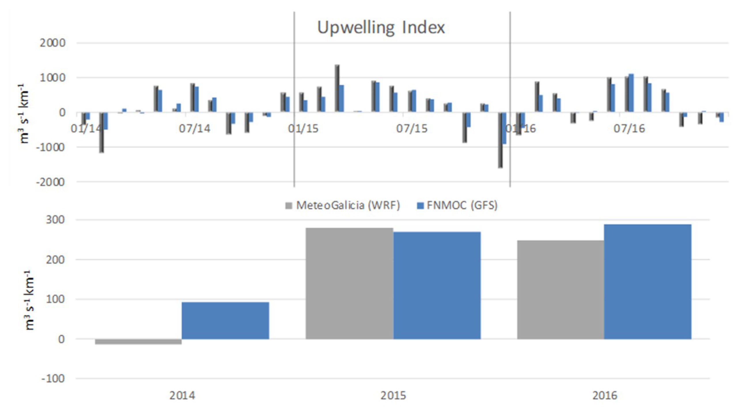
To evaluate interannual differences in the upwelling process, a time series of the upwelling index was analysed, derived from two meteorological models. Upwelling index time series was provided by the Spanish Institute of Oceanography (IEO) and was calculated using the sea level pressure obtained from the Spanish Meteorology Agency (Meteogalicia) WRF atmospheric model and from the Fleet Numerical Meteorology and Oceanography Center (FNMOC) GFS atmospheric model. Data were obtained for a site located off Roca Cape. The upwelling index was considerably lower in 2014 (<100 m3 s−1 km−1) compared with the following years, which presented very similar annual average values (≈300 m3 s−1 km−1) (Figure 9). The surface seawater temperature drop in the upwelling region can be detected by remote sensing since the upwelled water is characterized by lower temperature comparing to the surrounding seawater. Although satellite products and MOHID results allow identifying the part of the coastal area where the upwelling process occurred, this phenomenon is more evident in ODYSEEA and MOHID, where a dark blue strip parallel to the N-S shoreline is clearly visible, which corresponds to upwelled water (Figure 8). Furthermore, the visual analysis of this figure also allows concluding that upwelling was less intense in 2014 than in the subsequent years analysed.
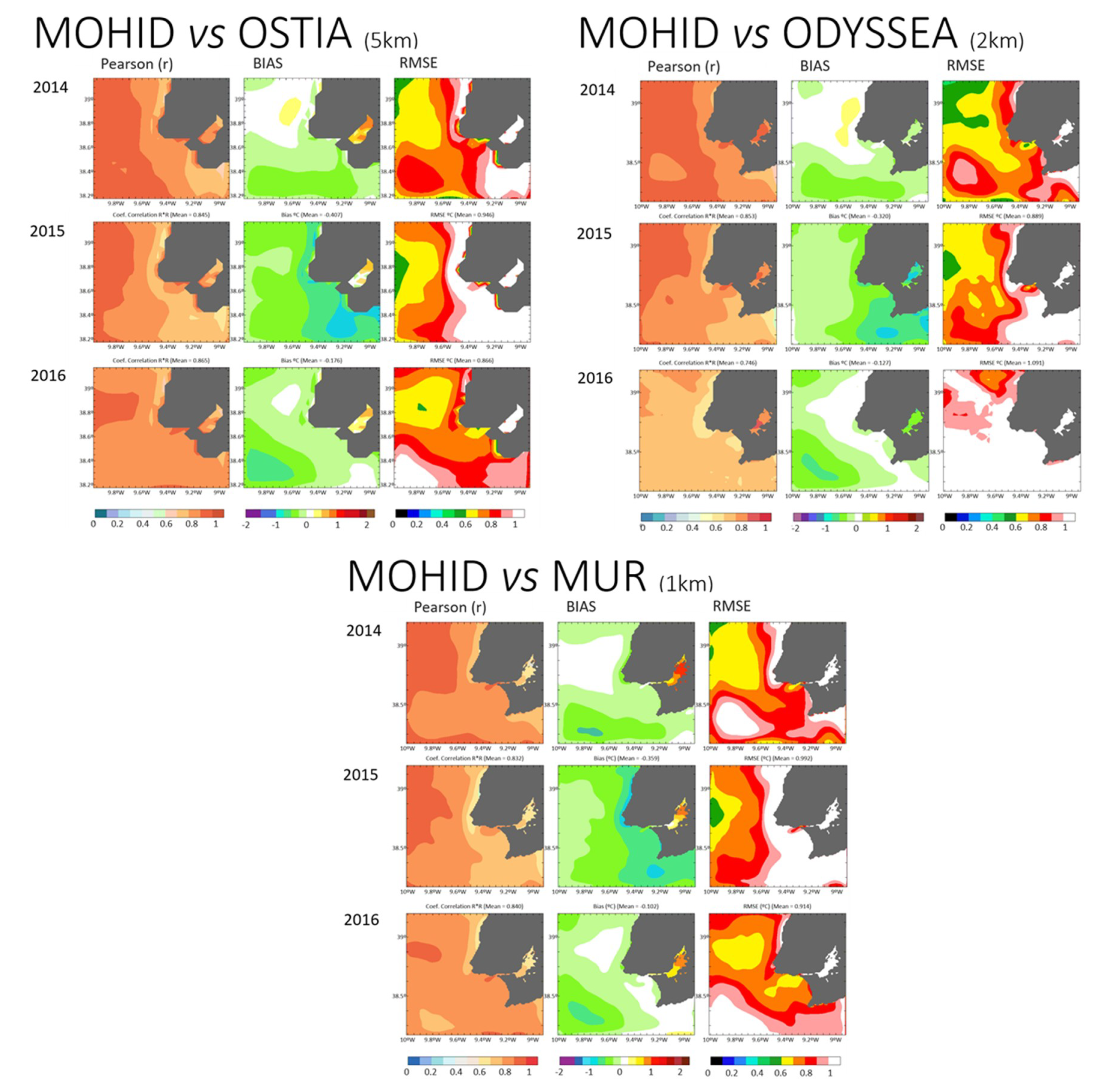
The Pearson correlation coefficients (r) obtained were very high and always superior to 0.86, indicating a very strong relationship between MOHID and the remote sensing products (Table 5). Regarding BIAS, the differences between modelling results and products data were always low and varied between −0.407 and −0.102 (Table 5). For all comparison, the RMSE error was always lower than 1 and higher than 0.7, which also indicates high accuracy of MOHID results. These results show that MOHID captures well the dominant pattern of the horizontal superficial distribution of the surface seawater temperature.
Values in Table 5 represent the mean of the statistical parameters for the entire study domain, but by plotting the spatial distribution of errors it is possible to observe where the differences are found.
Figure 10 shows that these differences (BIAS and RMSE) are more noticeable within the estuary and nearshore, in particular for OSTIA and MUR products that cannot capture the SST gradient. This can also be observed in Figure 8. MOHID and ODYSSEA present a similar distribution pattern of the differences, with BIAS always below 1 °C, including in the estuarine area.
Overall results indicate that the study area is characterized by the recurrent occurrence of upwelling event, which is well reproduced by the model. Therefore, it can be concluded that even in an extremely complex coastal area, as it is a TagusROFI domain, the MOHID Water model is adequately implemented and able to reproduce vertical stratification and horizontal patterns of SST. Moreover, of the three satellite products analysed in the present study, only ODYSSEA reproduces with accuracy upwelling events. Nevertheless, satellite data cannot be used to predict upwelling events as final filtered images are usually only available the next day but can be used to confirm an upwelling event represented by the model. On the contrary, 3D-MOHID Water is running operationally in forecasting mode, forecasting 3 days in every daily simulation.
4. Conclusions
Regions of freshwater influence (ROFIs) are interface areas between terrestrial freshwaters sources and the ocean, where physical processes characteristic of both estuaries and of coastal areas often occur and overlap, making these areas very complex systems. The spatiotemporal scales of these systems are so large and complex that the collection of in situ and/or spatial data alone cannot explain the processes that characterize them. This can be overcome using numerical models that despite being an approximation of the reality, provide a continuous representation in time and space of the system variables. More than giving a better understanding of the interactions between the various components of the system, these models are essential for the monitoring and management of the costal systems and associated resources. Nevertheless, the robustness of model-derived products to address specific scientific and management issues depends on its accuracy. Models assume properties for which no measurements are available and have known inherent uncertainties (e.g., model simplifications, mesh generation, roughness definition, etc.) [88]. Therefore, to minimize these uncertainties models are systematically calibrated by comparing modelling results with monitoring data. Apart from calibration, models should also be validated so as to determine the uncertainty associated with their solutions.
In the present work, the 3D-MOHID Water model was validated for the TagusROFI domain by comparing modelling results with in situ data (water level, surface seawater temperature (SST), salinity, and current direction and velocity) and SST remote sensing gridded L4 products (OSTIA, ODYSSEA, and MUR). These variables were chosen in the validation process because they are the most important hydrodynamics indicators with matching measured data. Indeed, the divergence of the horizontal flux (measurable through the propagation of the tide), in situ measurements of the velocity in water column, and the transport of conservative tracers (e.g., salinity) or of tracers with temporal variability lower than the tide (e.g., seawater temperature), are paramount parameters used to validate hydrodynamics. Seawater temperature and salinity are responsible for water density variability, which plays a central role in flow conditions in ROFI areas. Flow, however, can only be directly characterised with velocity fields and these can only be described through hydrodynamic models.
The statistical analyses used in validation include the calculation of the Pearson’s coefficient of correlation, BIAS index and RMES. Validation against two tidal gauges located at Cascais (coastal area) and at Lisbon (estuarine area) showed that the model is able to simulate observed water levels with accuracy, reproducing the amplitude and tidal phase, as well as its distortion during the propagation of the tidal wave within the estuary. Since the modelling results are accurate, it can be assumed that the model reproduces satisfactorily the horizontal flux divergence. A very good agreement between predictions of SST and salinity, and data from a CTD was also observed. The validation of current direction and velocity results using ADCP data indicated a high model accuracy for these variables. Finally, comparisons between model and satellite L4 products for SST showed that the model produces realistic SSTs and upwelling events. Although the use of more in-situ data would be desirable to increase spatial coverage, in the present paper it was used the most accurate data available. Notwithstanding, overall results showed that the 3D-MOHID Water setup and parametrisations were well implemented for the TagusROFI domain leading to highly accurate simulations. These results are even more important when a 3D model is used in simulations due to its complexity once it considers both horizontal and vertical discretization permitting a better representation of the heat and salinity fluxes in the water column. The validation of the 3D-MOHID Water is important because hydrodynamics is the basis for the transport of any biogeochemical variable through advection and/or diffusion processes, from the eulerian and langrangian point of view, and also indicates that it is robust enough to run in operational mode, including its forecast ability. Therefore, the 3D-MOHID can be considered an important management tool. Future research should be directed to the validation of the model’s biogeochemical component, and to the study of the biogeochemical processes in the TagusROFI domain. Moreover, it would be interesting to couple process-based-models (such as MOHID) with data-driven models [89] that employs machine learning techniques. This approach consists in feeding data-driven models with data from process-based-models that were already validated. Although this hybrid approach is still in its infancy in what concerns hydrodynamics due to the complexity and variability of the inherent processes, it could be a useful approach in the coming future. The results of the present work constitute an important step towards the implementation of this innovative approach.
Author Contributions
Conceptualization, H.d.P.; methodology, H.d.P., J.S., M.G., F.C.; validation, H.d.P.; formal analysis, H.d.P., M.G.; investigation, H.d.P., J.S., M.G., F.C.; writing—original draft preparation, H.d.P.; writing—review and editing, H.d.P., J.S., F.C., M.J., R.N.; visualization, H.d.P; project administration, R.N.
Funding
The present work was performed within the framework of the research projects “Tackling Marine Litter in the Atlantic Area (CleanAtlantic)” and “Innovation in the framework of the Atlantic deep ocean (iFADO)”, funded by the Interreg IVB—Atlantic Arc Programme and co-financed by the European Regional Development Fund (ERDF).
Acknowledgments
The authors would like to acknowledge the Portuguese Hydrographic Institute (IH) for kindly providing data on the water level in the study area and the E.U. Copernicus Marine Service Information and Satellite Monitoring of the Northwest Shelf Sea for providing the ODYSSEA SST product. Acknowledgements are also due to the Group for High Resolution Sea Surface Temperature (GHRSST) Multi-scale Ultra-high Resolution (MUR) and Operational Sea Surface Temperature and Sea Ice Analysis (OSTIA), the NASA EOSDIS Physical Oceanography Distributed Active Archive Center (PO.DAAC) at the Jet Propulsion Laboratory, Pasadena, CA (https://doi.org/10.5067/GHGMR-4FJ01 and https://doi.org/10.5067/GHOST-4FK01, respectively) from which SST data were obtained. We also would like to thank the Spanish Oceanographic Institute for providing upwelling data (www.marnaraia.com). A special thanks to Miguel Gaspar from IPMA for his crucial review of the paper. Thanks are also due to André Carvalho for helping with the Figures. The authors would like to acknowledge two anonymous referees for their valuable comments that improved the final version of the paper.
Conflicts of Interest
The authors declare no conflict of interest.
References
- Lakhan, V.C.; Trenhaile, A.S. Models and the Coastal System. In Elsevier Oceanography Series; Lakhan, A.S., Trenhaile, V.C., Eds.; Elsevier: Amsterdam, The Netherlands, 1989; Volume 49, pp. 1–16. [Google Scholar]
- Murthy, C.R.; Sinha, P.C.; Rao, Y.R. Modelling and monitoring of coastal marine processes. In Modelling and Monitoring of Coastal Marine Processes; Capital Publishing Company: New Delhi, India, 2008; pp. 1–246. [Google Scholar]
- Iglesias, I.; Avilez-Valente, P.; Luís Pinho, J.; Bio, A.; Manuel Vieira, J.; Bastos, L.; Veloso-Gomes, F. Numerical Modeling Tools Applied to Estuarine and Coastal Hydrodynamics: A User Perspective. In Coastal and Marine Environments—Physical Processes and Numerical Modelling; Intechopen: London, UK, 2019; p. 20. [Google Scholar]
- Petihakis, G.; Triantafyllou, G.; Korres, G.; Tsiaras, K.; Theodorou, A. Ecosystem modelling: Towards the development of a management tool for a marine coastal system part-II, ecosystem processes and biogeochemical fluxes. J. Mar. Syst. 2012, 94, S49–S64. [Google Scholar] [CrossRef]
- Lazure, P.; Garnier, V.; Dumas, F.; Herry, C.; Chifflet, M. Development of a hydrodynamic model of the Bay of Biscay. Validation of hydrology. Cont. Shelf Res. 2009, 29, 985–997. [Google Scholar] [CrossRef] [Green Version]
- Gunn, K.; Stock-Williams, C. On validating numerical hydrodynamic models of complex tidal flow. Int. J. Mar. Energy 2013, 3, e82–e97. [Google Scholar] [CrossRef]
- Guerreiro, M.; Fortunato, A.B.; Freire, P.; Rilo, A.; Taborda, R.; Freitas, M.C.; Andrade, C.; Silva, T.; Rodrigues, M.; Bertin, X.; et al. Evolution of the hydrodynamics of the Tagus estuary (Portugal) in the 21st century. Revista de Gestão Costeira Integrada-Journal of Integrated Coastal Zone Management 2014, 15, 65–80. [Google Scholar] [CrossRef]
- Cucco, A.; Quattrocchi, G.; Olita, A.; Fazioli, L.; Ribotti, A.; Sinerchia, M.; Tedesco, C.; Sorgente, R. Hydrodynamic modelling of coastal seas: The role of tidal dynamics in the Messina Strait, Western Mediterranean Sea. Nat. Hazards Earth Syst. Sci. 2016, 16, 1553–1569. [Google Scholar] [CrossRef]
- Gaeta, M.G.; Samaras, A.G.; Federico, I.; Archetti, R.; Maicu, F.; Lorenzetti, G. A coupled wave-3-D hydrodynamics model of the Taranto Sea (Italy): A multiple-nesting approach. Nat. Hazards Earth Syst. Sci. 2016, 16, 2071–2083. [Google Scholar] [CrossRef]
- Sedigh, M.; Tomlinson, R.; Cartwright, N.; Etemad-Shahidi, A. Numerical modelling of the Gold Coast Seaway area hydrodynamics and littoral drift. Ocean Eng. 2016, 121, 47–61. [Google Scholar] [CrossRef]
- Wild-allen, K.; Andrewartha, J. Connectivity between estuaries in fl uences nutrient transport, cycling and water quality. Mar. Chem. 2016, 185, 12–26. [Google Scholar] [CrossRef]
- Yin, Y.; Karunarathna, H.; Reeve, D.E. Numerical modelling of hydrodynamic and morphodynamic response of a meso-tidal estuary inlet to the impacts of global climate variabilities. Mar. Geol. 2019, 407, 229–247. [Google Scholar] [CrossRef]
- Garneau, C.; Duchesne, S.; St-Hilaire, A. Comparison of modelling approaches to estimate trapping efficiency of sedimentation basins on peatlands used for peat extraction. Ecol. Eng. 2019, 133, 60–68. [Google Scholar] [CrossRef]
- Restrepo, J.C.; Escobar, J.; Otero, L.; Franco, D.; Pierini, J.; Correa, I. Factors Influencing the Distribution and Characteristics of Surface Sediment in the Bay of Cartagena, Colombia. J. Coast. Res. 2016, 331, 135–148. [Google Scholar] [CrossRef]
- Ospino, S.; Restrepo, J.C.; Otero, L.; Pierini, J.; Alvarez-Silva, O. Saltwater Intrusion into a River with High Fluvial Discharge: A Microtidal Estuary of the Magdalena River, Colombia. J. Coast. Res. 2018, 34, 1273–1288. [Google Scholar] [CrossRef]
- Franz, G.A.S.; Leitão, P.; dos Santos, A.; Juliano, M.; Neves, R. From regional to local scale modelling on the south-eastern Brazilian shelf: Case study of Paranaguá estuarine system. Braz. J. Oceanogr. 2016, 64, 277–294. [Google Scholar] [CrossRef]
- Angeletti, S.; Pierini, J.O.; Cervellini, P.M. Suspended sediment contribution resulting from bioturbation in intertidal sites of a SW Atlantic mesotidal estuary: Data analysis and numerical modelling. Sci. Mar. 2019, 82, 245–256. [Google Scholar] [CrossRef]
- Pierini, J.O.; Campuzano, F.J.; Leitão, P.C.; Gómez, E.A.; Neves, R.J. Atmospheric Influence Over the Residence Time in the Bahia Blanca Estuary, Argentina. Thalassas 2019, 35, 275–286. [Google Scholar] [CrossRef]
- Alonso, R.; Jackson, M.; Santoro, P.; Fossati, M.; Solari, S.; Teixeira, L. Wave and tidal energy resource assessment in Uruguayan shelf seas. Renew. Energy 2017, 114, 18–31. [Google Scholar] [CrossRef]
- Saraiva, S.; Fernandes, L.; van der Meer, J.; Neves, R.; Kooijman, S.A.L.M. The role of bivalves in the Balgzand: First steps on an integrated modelling approach. Ecol. Mod. 2017, 359, 34–48. [Google Scholar] [CrossRef] [Green Version]
- Ascione Kenov, I.; Muttin, F.; Campbell, R.; Fernandes, R.; Campuzano, F.; Machado, F.; Franz, G.; Neves, R. Water fluxes and renewal rates at Pertuis d’Antioche/Marennes-Oléron Bay, France. Estuar. Coast. Shelf Sci. 2015, 167, 32–44. [Google Scholar] [CrossRef]
- Muttin, F.; Campbell, R.; Ouansafi, A.; Benelmostafa, Y. Numerical modelling and full-scale exercise of oil-spill containment boom on Galician coast. Int. J. Comput. Methods Exp. Meas. 2017, 5, 760–770. [Google Scholar] [CrossRef]
- Galesic, M.; Andricevic, R.; Gotovac, H.; Srzic, V. Concentration statistics of solute transport for the near field zone of an estuary. Adv. Water Resour. 2016, 94, 424–440. [Google Scholar] [CrossRef]
- Salamena, G.G.; Martins, F.; Ridd, P.V. The density-driven circulation of the coastal hypersaline system of the Great Barrier Reef, Australia. Mar. Pollut. Bull. 2016, 105, 277–285. [Google Scholar] [CrossRef]
- Li, Y.; Martins, F.; Wolanski, E. Sensitivity analysis of the physical dynamics of the Fly River plume in Torres Strait. Estuar. Coast. Shelf Sci. 2017, 194, 84–91. [Google Scholar] [CrossRef]
- Bartolomeu, S.; Malhadas, M.S.; Ribeiro, J.; Leitão, P.C.; Dias, J.M. Influence of MeteOcean processes on MSYM sea level predictions in the Malacca Straits. Mod. Manag. Forum 2018, 2, 1–17. [Google Scholar] [CrossRef]
- Lee, J.-H.; Lim, B.-J.; Kim, D.-Y.; Park, S.-H.; Chang, Y.-S. The Validation of MOHID Regional Ocean Circulation Model around the East Asian Seas in 2016. J. Korean Earth Sci. Soc. 2018, 39, 436–457. [Google Scholar] [CrossRef]
- Campuzano, F.; Brito, D.; Juliano, M.; Fernandes, R.; de Pablo, H.; Neves, R. Coupling watersheds, estuaries and regional ocean through numerical modelling for Western Iberia: A novel methodology. Ocean Dyn. 2016, 66, 1745–1756. [Google Scholar] [CrossRef]
- Silva, A.; Pinto, L.; Rodrigues, S.M.; de Pablo, H.; Santos, M.; Moita, T.; Mateus, M. A HAB warning system for shellfish harvesting in Portugal. Harmful Algae 2016, 53, 33–39. [Google Scholar] [CrossRef]
- Janeiro, J.; Neves, A.; Martins, F.; Relvas, P. Integrating technologies for oil spill response in the SW Iberian coast. J. Mar. Syst. 2017, 173, 31–42. [Google Scholar] [CrossRef] [Green Version]
- Valentim, J.M.; Vaz, N.; Silva, H.; Duarte, B.; Caçador, I.; Dias, J.M. Tagus estuary and Ria de Aveiro salt marsh dynamics and the impact of sea level rise. Estuar. Coast. Shelf Sci. 2013, 130, 138–151. [Google Scholar] [CrossRef]
- Fernandes, R.; Braunschweig, F.; Lourenço, F.; Neves, R. Combining operational models and data into a dynamic vessel risk assessment tool for coastal regions. Ocean Sci. 2016, 12, 285–317. [Google Scholar] [CrossRef] [Green Version]
- Gaspar, R.; Marques, L.; Pinto, L.; Baeta, A.; Pereira, L.; Martins, I.; Marques, J.C.; Neto, J.M. Origin here, impact there—The need of integrated management for river basins and coastal areas. Ecol. Indic. 2017, 72, 794–802. [Google Scholar] [CrossRef]
- Vargas, C.I.C.; Vaz, N.; Dias, J.M. An evaluation of climate change effects in estuarine salinity patterns: Application to Ria de Aveiro shallow water system. Estuar. Coast. Shelf Sci. 2017, 189, 33–45. [Google Scholar] [CrossRef]
- Martins, I.; Dias, E.; Ilarri, M.I.; Campuzano, F.J.; Pinto, L.; Santos, M.M.; Antunes, C. Antagonistic effects of multiple stressors on macroinvertebrate biomass from a temperate estuary (Minho estuary, NW Iberian Peninsula). Ecol. Indic. 2019, 101, 792–803. [Google Scholar] [CrossRef]
- Portela, L.I.; Neves, R. Numerical modelling of suspended sediment transport in tidal estuaries: A comparison between the Tagus (Portugal) and the Scheldt (Belgium-the Netherlands). Neth. J. Aquat. Ecol. 1994, 28, 329–335. [Google Scholar] [CrossRef]
- Franz, G.; Pinto, L.; Ascione, I.; Mateus, M.; Fernandes, R.; Leitão, P.; Neves, R. Modelling of cohesive sediment dynamics in tidal estuarine systems: Case study of Tagus estuary, Portugal. Estuar. Coast. Shelf Sci. 2014, 151, 34–44. [Google Scholar] [CrossRef]
- Franz, G.; Leitão, P.; Pinto, L.; Jauch, E.; Fernandes, L.; Neves, R. Development and validation of a morphological model for multiple sediment classes. Int. J. Sediment Res. 2017, 32, 585–596. [Google Scholar] [CrossRef]
- Mateus, M.; Neves, R. Evaluating light and nutrient limitation in the Tagus estuary using a process-oriented ecological model. Proc. Inst. Mar. Eng. Sci. Technol. Part A J. Mar. Eng. Technol. 2008, 32, 585–592. [Google Scholar] [CrossRef]
- Mateus, M.; Riflet, G.; Chambel, P.; Fernandes, L.; Fernandes, R.; Juliano, M.; Campuzano, F.; de Pablo, H.; Neves, R. An operational model for the West Iberian coast: Products and services. Ocean Sci. 2012, 8, 713–732. [Google Scholar] [CrossRef]
- Viegas, C.; Neves, R.; Fernandes, R.; Mateus, M. Modelling tools to support an early alert system for bathing water quality. Environ. Eng. Manag. J. 2012, 11, 907–918. [Google Scholar] [CrossRef]
- Viegas, C.; Nunes, S.; Fernandes, R.; Neves, R. Streams contribution on bathing water quality after rainfall events in Costa do Estoril- a tool to implement an alert system for bathing water quality. J. Coast. Res. 2015, 56, 1961–1965. [Google Scholar]
- Canas, A.; Santos, A.; Leitao, P. Effect of large scale atmospheric pressure changes on water level in the tagus estuary. J. Coast. Res. 2009, 56, 1627–1631. [Google Scholar]
- Braunschweig, F.; Martins, F.; Chambel, P.; Neves, R. A methodology to estimate renewal time scales in estuaries: The Tagus Estuary case. Ocean Dyn. 2003, 53, 137–145. [Google Scholar] [CrossRef]
- Oliveira, A.P.; Mateus, M.D.; Cabeçadas, G.; Neves, R. Water-air CO2 fluxes in the Tagus estuary plume (Portugal) during two distinct winter episodes. Carbon Balance Manag. 2015, 10, 1–15. [Google Scholar] [CrossRef]
- Vaz, N.; Fernandes, L.; Leitão, P.C.; Dias, J.M.; Neves, R.; Manuel, A. The Tagus estuarine plume induced by wind and river runoff: Winter 2007 case study. J. Coast. Res. 2009, 56, 1090–1094. [Google Scholar]
- Vaz, N.; Rodrigues, J.G.; Mateus, M.; Franz, G.; Campuzano, F.; Neves, R.; Dias, J.M. Subtidal variability of the Tagus river plume in winter 2013. Sci. Total Environ. 2018, 627, 1353–1362. [Google Scholar] [CrossRef]
- Otero, P.; Ruiz-Villarreal, M.; Peliz, A. Variability of river plumes off Northwest Iberia in response to wind events. J. Mar. Syst. 2008, 72, 238–255. [Google Scholar] [CrossRef]
- Oliveira, P.B.; Nolasco, R.; Dubert, J.; Moita, T.; Peliz, Á. Surface temperature, chlorophyll and advection patterns during a summer upwelling event off central Portugal. Cont. Shelf Res. 2009, 29, 759–774. [Google Scholar] [CrossRef]
- Stansby, P.K. Coastal hydrodynamics—Present and future. J. Hydraul. Res. 2013, 51, 341–350. [Google Scholar] [CrossRef]
- Refsgaard, J.C. Parameterisation, calibration and validation of distributed hydrological models. J. Hydrol. 1997, 198, 69–97. [Google Scholar] [CrossRef]
- Legates, D.R.; McCabe, G.J. Evaluating the use of “goodness-of-fit” measures in hydrologic and hydroclimatic model validation. Water Resour. Res. 1999, 35, 233–241. [Google Scholar] [CrossRef]
- Moriasi, D.N.; Arnold, J.G.; Van Liew, M.W.; Bingner, R.L.; Harmel, R.D.; Veith, T.L. Model Evaluation Guidelines for Systematic Quantification of Accuacy in Watershed Simulation. Am. Soc. Agric. Biol. Eng. 2007, 50, 885–900. [Google Scholar] [CrossRef]
- Rosen, S.D. Recommended methodology and considerations for acceptance of the calibration and validation of a hydrodynamic model. In Proceedings of the 40th CIESM Congress, Marseille, France, 28 October–1 November 2013. [Google Scholar]
- Williams, J.J.; Esteves, L.S. Guidance on Setup, Calibration, and Validation of Hydrodynamic, Wave, and Sediment Models for Shelf Seas and Estuaries. Adv. Civ. Eng. 2017, 2017, 1–25. [Google Scholar] [CrossRef]
- Valente, A.S.; da Silva, J.C.B. On the observability of the fortnightly cycle of the Tagus estuary turbid plume using MODIS ocean colour images. J. Mar. Syst. 2009, 75, 131–137. [Google Scholar] [CrossRef]
- Fortunato, A.B.; Baptista, A.M.; Luettich, R.A. A three-dimensional model of tidal currents in the mouth of the Tagus estuary. Cont. Shelf Res. 1997, 17, 1689–1714. [Google Scholar] [CrossRef]
- Fernández-Nóvoa, D.; Gómez-Gesteira, M.; Mendes, R.; DeCastro, M.; Vaz, N.; Dias, J.M. Influence of main forcing affecting the Tagus turbid plume under high river discharges using MODIS imagery. PLoS ONE 2017, 12, 1–27. [Google Scholar] [CrossRef]
- Fortunato, A.B.; Oliveira, A.; Baptista, A.M. On the effect of tidal flats on the hydrodynamics of the Tagus estuary. Oceanol. Acta 1999, 22, 31–44. [Google Scholar] [CrossRef] [Green Version]
- Fortunato, A.B.; Freire, P.; Bertin, X.; Rodrigues, M.; Ferreira, J.; Liberato, M.L.R. A numerical study of the February 15, 1941 storm in the Tagus estuary. Cont. Shelf Res. 2017, 144, 50–64. [Google Scholar] [CrossRef]
- Jouanneau, J.M.; Garcia, C.; Oliveira, A.; Rodrigues, A.; Dias, J.A.; Weber, O. Dispersal and deposition of suspended sediment on the shelf off the Tagus and Sado estuaries, S.W. Portugal. Prog. Oceanogr. 1998, 42, 233–257. [Google Scholar] [CrossRef]
- Stanley, D.J. La plate-forme continentale du Portugal et les provinces adjacentes: Analyse géomorphologique. Geo Mar. Lett. 1982, 2, 109. [Google Scholar] [CrossRef]
- Gameiro, C.; Cartaxana, P.; Brotas, V. Environmental drivers of phytoplankton distribution and composition in Tagus Estuary, Portugal. Estuar. Coast. Shelf Sci. 2007, 75, 21–34. [Google Scholar] [CrossRef]
- Neves, F. Dynamics and Hydrology of the Tagus estuary: Results from In Situ Observations. Ph.D. Thesis, Universidade de Lisboa, Lisbon, Portugal, 2010. [Google Scholar]
- Rodrigues, R. The Tagus Estuarine Plume Variability: Impact in Coastal Circulation and Hydrography. Master’s Thesis, University of Aveiro, Aveiro, Portugal, 2015. [Google Scholar]
- Rusu, L.; Bernardino, M.; Guedes Soares, C. Modelling the influence of currents on wave propagation at the entrance of the Tagus estuary. Ocean Eng. 2011, 38, 1174–1183. [Google Scholar] [CrossRef]
- Vaz, N.; Mateus, M.; Plecha, S.; Sousa, M.C.; Leitão, P.C.; Neves, R.; Dias, J.M. Modeling SST and chlorophyll patterns in a coupled estuary-coastal system of Portugal: The Tagus case study. J. Mar. Syst. 2015, 147, 123–137. [Google Scholar] [CrossRef]
- Fiúza, A.F.G.; Macedo, M.E.; Guerreiro, M.R. Climatological space and time variation of the Portuguese coastal upwelling. Oceanol. Acta 1982, 5, 31–40. [Google Scholar]
- Ambar, I.; Fiúza, A. Some Features of the Portugal Current System: A poleward slope undercurrent, an upwelling-related summer southward flow and an autumn-winter poleward coastal surface current. In Proceedings of the 2nd International Conference on Air-Sea Interaction and on Meteorology and Oceanography, Boston, MA, USA, 18–22 September 1994. [Google Scholar]
- Fiúza, A.F.G. Upwelling patterns off Portugal. In Coastal Upwelling Its Sediment Record; Springer: New York, NY, USA, 1983; pp. 85–98. [Google Scholar] [CrossRef]
- Ruiz-Villarreal, M. Hydrodynamic Model Study of the Ria de Pontevedra Under Estuarine Conditions. Estuar. Coast. Shelf Sci. 2002, 54, 101–113. [Google Scholar] [CrossRef]
- Moita, M.T.; Oliveira, P.B.; Mendes, J.C.; Palma, A.S. Distribution of chlorophyll a and Gymnodinium catenatum associated with coastal upwelling plumes off central Portugal. Acta Oecol. 2003, 24, 125–132. [Google Scholar] [CrossRef]
- Blazek, J. Principles of Solution of the Governing Equations. In Computational Fluid Dynamics: Principles and Applications, 3rd ed.; Blazek, J., Ed.; Elsevier Science: San Diego, CA, USA, 2015; pp. 121–166. [Google Scholar]
- Millero, F.J.; Poisson, A. International one-atmosphere equation of state of seawater. Deep Sea Res. Part A Oceanogr. Res. Pap. 1981, 28, 625–629. [Google Scholar] [CrossRef]
- Leitão, P.; Mateus, M.; Braunschweig, F.; Fernandes, L.; Neves, R. Modelling coastal systems: The MOHID Water numerical lab. In Perspectives on Integrated Coastal Zone Management in South America; Neves, R., Baretta, J., Mateus, M., Eds.; IST Press: Lisbon, Portugal, 2008; pp. 77–88. [Google Scholar]
- Lyard, F.; Lefevre, F.; Letellier, T.; Francis, O. Modelling the global ocean tides: Modern insights from FES2004. Ocean Dyn. 2006, 56, 394–415. [Google Scholar] [CrossRef]
- Campuzano, F.J.; Fernandes, R.; Leitão, P.C.; Viegas, C.; de Pablo, H.; Neves, R. Implementing local operational models based on an offline downscaling technique: The Tagus estuary case. In Proceedings of the 2.as Jornadas de Engenharia Hidrográfica, Lisbon, Portugal, 20–22 June 2012. [Google Scholar]
- Flather, R.A. A Tidal Model of the North-West European Continental Shelf. Mem. Soc. R. Sci. Liège 1976, 10, 141–164. [Google Scholar]
- Burchard, H.; Bolding, K.; Villarreal, M.R. GOTM, A General Ocean Turbulence Model; Report EUR18745 EN; Space Applications Institute: Athens, Greece, 1999. [Google Scholar]
- Trancoso, A.R. Operational Modelling as a Tool in Wind Power Forecasts and Meteorological Warnings. PhD Thesis, Universidade de Lisboa, Lisboa, Portugal, 2012. [Google Scholar]
- Carrere, L.; Lyard, F.; Cancet, M.; Roblou, L.; Guillot, A.; Roblou, L. FES 2012: A new global tidal model taking advantage of nearly 20 years of altimetry. In Proceedings of the 20 Years of Progress in Radar Altimetry, Venice, Italy, 24–29 September 2012. [Google Scholar]
- Drillet, Y.; Bourdallé-Badie, R.; Siefridt, L.; Le Provost, C. Meddies in the Mercator North Atlantic and Mediterranean Sea eddy-resolving model. J. Geophys. Res. C Ocean. 2005, 110, 1–16. [Google Scholar] [CrossRef]
- Grell, G.A.; Dudhia, J.S.D. A description of the fifth-generation Penn State/NCAR Mesoscale Model (MM5). NCAR Technical Note NCAR/TN-398+STR 1994. [Google Scholar] [CrossRef]
- Stark, J.D.; Donlon, C.J.; Martin, M.J.; McCulloch, M.E. OSTIA: An operational, high resolution, real time, global sea surface temperature analysis system. In Proceedings of the Oceans MTS/IEEE Conference, Vancouver, BC, Canada, 18–21 June 2007. [Google Scholar]
- Autret, E.; Paul, F.; Tandéo, P.; Hackett, B. For Level 3 and 4 ODYSSEA SST products over the global ocean and north western shelves—SST _ GLO _ SST _ L3 _ NRT _ OBSERVATIONS _ 010 _ 010—SST _ NWS _ SST _ L4 _ NRT _ OBSERVATIONS _ 010 _ 003, 2017; EU Copernicus Marine Service–Public: Brussels, Belgium.
- Martin, M.; Dash, P.; Ignatov, A.; Banzon, V.; Beggs, H.; Brasnett, B.; Cayula, J.F.; Cummings, J.; Donlon, C.; Gentemann, C.; et al. Group for High Resolution Sea Surface temperature (GHRSST) analysis fields inter-comparisons. Part 1: A GHRSST multi-product ensemble (GMPE). Deep. Res. Part II Top. Stud. Oceanogr. 2012, 77–80, 21–30. [Google Scholar] [CrossRef]
- Parkinson, C.L.; Ward, A.; King, M.D. Earth Science Reference Handbook; National Aeronautics and Space Administration: Washington, DC, USA, 2006. [Google Scholar]
- Glock, K.; Tritthart, M.; Habersack, H.; Hauer, C. Comparison of hydrodynamics simulated by 1D, 2D and 3D models focusing on bed shear stresses. Water 2019, 11, 226. [Google Scholar] [CrossRef]
- García-Alba, J.; Bárcena, J.F.; Ugarteburu, C.; García, A. Artificial neural networks as emulators of process-based models to analyse bathing water quality in estuaries. Water Res. 2019, 150, 283–295. [Google Scholar] [CrossRef]
Figure 1.
Map of the TagusROFI area showing the sites where environmental parameters were taken. HS–Hydrologic Station; LTG–Lisbon Tide Gauge; CTG–Cascais Tide Gauge; CTD–Conductivity, Temperature, and Depth probe; ADCP–Acoustic Doppler Current Profiler; MS–Meteorological Station.
Figure 1.
Map of the TagusROFI area showing the sites where environmental parameters were taken. HS–Hydrologic Station; LTG–Lisbon Tide Gauge; CTG–Cascais Tide Gauge; CTD–Conductivity, Temperature, and Depth probe; ADCP–Acoustic Doppler Current Profiler; MS–Meteorological Station.

Figure 2.
TagusROFI domain bathymetry. Colours represent the depth in meters (m) and land in grey. The colour scale is logarithmic.
Figure 2.
TagusROFI domain bathymetry. Colours represent the depth in meters (m) and land in grey. The colour scale is logarithmic.

Figure 3.
Left: Comparison of the observed (green dots) and simulated (blue dots) water levels at CTG (top) and LTG (bottom) stations. Difference between Observed and Modelled data. Right: Performance of the MOHID forecast for the TagusROFI. Model comparison vs tide gauge for CTG (top) and LTG (bottom) stations.

Figure 4.
Tidal wave lag between CTG (coastal area) and LTG (in the Tagus estuary) stations. Green dots and crosses represent observed data whereas blue lines represent the modelling results.
Figure 4.
Tidal wave lag between CTG (coastal area) and LTG (in the Tagus estuary) stations. Green dots and crosses represent observed data whereas blue lines represent the modelling results.

Figure 5.
Left: Comparison of the observed (green dots) and simulated (blue dots) surface seawater temperature (top) and salinity (bottom). Right: Performance of the MOHID Water results for the TagusROFI. Model vs CTD for surface seawater temperature (top) and salinity (bottom).
Figure 5.
Left: Comparison of the observed (green dots) and simulated (blue dots) surface seawater temperature (top) and salinity (bottom). Right: Performance of the MOHID Water results for the TagusROFI. Model vs CTD for surface seawater temperature (top) and salinity (bottom).

Figure 6.
Profiles comparison of the velocity module, velocity components u and v and directions between MOHID Water results (top) and ADCP data (down) in function of depth and time; and wind time-series. Data obtained off Cascais between 2 and 17 July 2009. For both observations and modelling results, the output was of 15 min.

Figure 7.
Profiles comparison between MOHID Water results (top) and ADCP data (bottom) for the velocity components u and v in function of depth. Data obtained off Cascais between 2 and 17 July 2009. Grey lines represent velocity at each instant of time measured or predicted, and blue and green lines represent the average trend.

Figure 8.
Interannual comparison of surface seawater temperature between MOHID and Satellite L4 gridded products (OSTIA-5km, ODYSSEA-2 km; and MUR 1 km) for the period 2014–2016.
Figure 8.
Interannual comparison of surface seawater temperature between MOHID and Satellite L4 gridded products (OSTIA-5km, ODYSSEA-2 km; and MUR 1 km) for the period 2014–2016.

Figure 9.
Upwelling index derived from WRF and GFS atmospheric models between 2014 and 2016.

Figure 10.
Spatial distribution of the differences between MOHID and the three satellite products (OSTIA, ODYSSEA, and MUR) for the Pearson correlation coefficient (r), BIAS and RMSE, between 2014–2016.
Figure 10.
Spatial distribution of the differences between MOHID and the three satellite products (OSTIA, ODYSSEA, and MUR) for the Pearson correlation coefficient (r), BIAS and RMSE, between 2014–2016.


Table 1.
Model configuration for the TagusROFI.
| Settings | Level 1 –WestIberia | Level2–PCOMS | Level 3-TagusROFI |
|---|---|---|---|
| Model characterization | 2D-Barotropic | 3D–Baroclinic | 3D-Baroclinic |
| Grid corners | 33.50° N–49.90° N 1.00° W–13.50° W | 34.38° N–45.00° N 12.60° W–5.50° W | 38.16° N–39.21° N 10.02° W–8.90° W |
| Cells dimension | 208 × 156 | 177 × 125 | 121 × 146 |
| Bathymetry | EMODneta Hydrography portal | EMODneta Hydrography portal | Delaunay triangulation with IH Data and GEBCO |
| Horizontal Grid | Regular: (≈5.7 km) | Regular: (≈5.7 km) | Irregular: 200 m to 2 km |
| Vertical Grid | 1 layer | 7 Sigma Layer (0 m–8.68 m) 43 Cartesian layers | 7 Sigma Layer (0 m–8.68 m) 43 Cartesian layers |
| Δt | 60 seconds | 60 seconds | 6 seconds |
| Tides | FES2004b & FES2012c | From Level1 | From Level2 |
| OBC Water | From MercatorOcéan PSY2V4 (Releases 1–4)d | From Level2 | |
| Assimilation | Flow relaxation scheme of 10 cells with a time decay of 1 week at the open boundary and 0 inside the domain | Flow relaxation scheme of 10 cells with a time decay of 1 week at the open boundary and 0 inside the domain | |
| OBC Atmosphere | MM5e (9 km) | MM5e (9 km) | WRFf (3 km) |
| Discharges | No | No | Tagus (hourly), Sorraia, Trancão and WWTP (monthly) |
| Turbulence | GOTMg | GOTMg | |
| Bottom | Rugosity of 0.0025 m2 s−1 | Rugosity of 0. 0025 m2 s−1 | Rugosity of 0. 0025 m2 s−1 |
Table 2.
Water level. Data summary and results of statistics used to assess the level of agreement between measured data and modelling results. n—number of observations; r—correlation coefficient; BIAS—Average bias; RMSE—Root mean square error.
Table 2.
Water level. Data summary and results of statistics used to assess the level of agreement between measured data and modelling results. n—number of observations; r—correlation coefficient; BIAS—Average bias; RMSE—Root mean square error.
| Tide Gauge | Average (min–max) MOHID | Average (min-max) Tide Gauge | n | Pearson (r) | BIAS | RMSE |
|---|---|---|---|---|---|---|
| CTG | 2.02 (0.39–3.73) | 2.02 (0.31–3.69) | 4445 | 0.995 | 0.003 | 0.17 |
| LTG | 2.01 (0.32–3.70) | 2.00 (0-17–3.77) | 4341 | 0.994 | 0.005 | 0.45 |
Table 3.
Surface seawater temperature and salinity. Data summary and results of statistics used to assess the level of agreement between measured data and modelling results. n—number of observations; r—correlation coefficient; BIAS—Average bias; RMSE—Root mean square error.
Table 3.
Surface seawater temperature and salinity. Data summary and results of statistics used to assess the level of agreement between measured data and modelling results. n—number of observations; r—correlation coefficient; BIAS—Average bias; RMSE—Root mean square error.
| Parameter | Average (min-max) MOHID | Average (min-max) CTD | n | Pearson (r) | BIAS | RMSE |
|---|---|---|---|---|---|---|
| Temperature | 14.2 (11.4–17.4) | 14.3 (11.9–17.3) | 21436 | 0.91 | 0.1 | 0.4 |
| Salinity | 28.0 (2.1–35.6) | 27.4 (1.3–35.3) | 21436 | 0.86 | –0.9 | 2.9 |
Table 4.
Current velocity and direction. Data summary and results of statistics used to assess the level of agreement between measured data and modelling results. n—number of observations; r—correlation coefficient; BIAS—Average bias; RMSE—Root mean square error.
Table 4.
Current velocity and direction. Data summary and results of statistics used to assess the level of agreement between measured data and modelling results. n—number of observations; r—correlation coefficient; BIAS—Average bias; RMSE—Root mean square error.
| Average (min-max) MOHID | Average (min-max) ADCP | n | Pearson (r) | BIAS | RMSE | |
|---|---|---|---|---|---|---|
| Depth (2.5 m–15 m) | ||||||
| Vel. Modulus (m s−1) | 0.16 (0.0087–0.41) | 0.17 (0.0054–0.43) | 1440 | 0.68 | 0.014 | 0.10 |
| Direction (rad) | 151 (0.2–360) | 134 (2.4–359) | 0.63 | –9.8 | 45 | |
| Velocity u (m s−1) | 0.097 (−0.069–0.30) | 0.099 (−0.14–0.34) | 0.63 | 0.0019 | 0.092 | |
| Velocity v (m s−1) | −0.089 (−0.38–0.11) | −0.11 (−0.43–0.11) | 0.73 | −0.025 | 0.11 | |
| Depth (15 m–30 m) | ||||||
| Vel. Modulus (m s−1) | 0.10 (0.0039–0.30) | 0.12 (0.0025–0.34) | 1440 | 0.62 | 0.018 | 0.065 |
| Direction (rad) | 151 (0.2–360) | 164 (2–358) | 0.66 | –14 | 50 | |
| Velocity u (m s−1) | 0.084 (−0.046–0.30) | 0.092 (−0.086–0.29) | 0.63 | 0.0082 | 0.066 | |
| Velocity v (m s−1) | −0.052 (−0.15–0.098) | −0.035 (−0.26–0.13) | 0.71 | –0.029 | 0.071 |
Table 5.
Surface seawater temperature from satellite data. Data summary and results of statistics used to assess the level of agreement between remote sensing data and modelling results. n–number of observations; r–correlation coefficient; BIAS–Average bias; RMSE–Root mean square error.
Table 5.
Surface seawater temperature from satellite data. Data summary and results of statistics used to assess the level of agreement between remote sensing data and modelling results. n–number of observations; r–correlation coefficient; BIAS–Average bias; RMSE–Root mean square error.
| Year | Satellite | Average MOHID | Average L4 products | n (per day) | Pearson (r) | BIAS | RMSE |
|---|---|---|---|---|---|---|---|
| 2014 | OSTIA | 17.11 | 17.18 | 355 | 0.937 | −0.064 | 0.846 |
| ODYSSEA | 17.11 | 17.17 | 2095 | 0.948 | −0.059 | 0.773 | |
| MUR | 17.12 | 17.20 | 8356 | 0.934 | −0.078 | 0.894 | |
| 2015 | OSTIA | 16.50 | 16.91 | 255 | 0.919 | −0.407 | 0.946 |
| ODYSSEA | 16.51 | 16.83 | 2095 | 0.924 | −0.320 | 0.889 | |
| MUR | 16.56 | 16.87 | 8356 | 0.912 | −0.359 | 0.992 | |
| 2016 | OSTIA | 16.74 | 16.19 | 355 | 0.930 | −0.176 | 0.866 |
| ODYSSEA | 16.71 | 16.83 | 2095 | 0.864 | −0.127 | 0.978 | |
| MUR | 16.73 | 16.83 | 8356 | 0.916 | −0.102 | 0.914 |
© 2019 by the authors. Licensee MDPI, Basel, Switzerland. This article is an open access article distributed under the terms and conditions of the Creative Commons Attribution (CC BY) license (http://creativecommons.org/licenses/by/4.0/).
Share and Cite
MDPI and ACS Style
de Pablo, H.; Sobrinho, J.; Garcia, M.; Campuzano, F.; Juliano, M.; Neves, R. Validation of the 3D-MOHID Hydrodynamic Model for the Tagus Coastal Area. Water 2019, 11, 1713. https://doi.org/10.3390/w11081713
AMA Style
de Pablo H, Sobrinho J, Garcia M, Campuzano F, Juliano M, Neves R. Validation of the 3D-MOHID Hydrodynamic Model for the Tagus Coastal Area. Water. 2019; 11(8):1713. https://doi.org/10.3390/w11081713
Chicago/Turabian Stylede Pablo, Hilda, João Sobrinho, Mariangel Garcia, Francisco Campuzano, Manuela Juliano, and Ramiro Neves. 2019. "Validation of the 3D-MOHID Hydrodynamic Model for the Tagus Coastal Area" Water 11, no. 8: 1713. https://doi.org/10.3390/w11081713
Note that from the first issue of 2016, this journal uses article numbers instead of page numbers. See further details here.