Inter-Comparison of Different Bayesian Model Averaging Modifications in Streamflow Simulation

1
Department of Civil Engineering, McMaster University, 1280 Main Street West, Hamilton, ON L8S 4L7, Canada
2
School of Geography and Earth Sciences, McMaster University, 1280 Main Street West, Hamilton, ON L8S 4L7, Canada
3
United Nations University Institute for Water, Environment, and Health, Hamilton, ON L8P 0A1, Canada
*
Author to whom correspondence should be addressed.
Water 2019, 11(8), 1707; https://doi.org/10.3390/w11081707
Submission received: 16 June 2019
/
Revised: 9 August 2019
/
Accepted: 13 August 2019
/
Published: 16 August 2019
(This article belongs to the Section Hydrology)
Abstract
:Bayesian model averaging (BMA) is a popular method using the advantages of forecast ensemble to enhance the reliability and accuracy of predictions. The inherent assumptions of the classical BMA has led to different variants. However, there is not a comprehensive examination of how these solutions improve the original BMA in the context of streamflow simulation. In this study, a scenario-based analysis was conducted for assessment of various modifications and how they affect BMA results. The evaluated modifications included using various streamflow ensembles, data transformation procedures, distribution types, standard deviation forms, and optimization methods. We applied the proposed analysis in two data-poor watersheds located in northern Ontario, Canada. The results indicate that using more representative distribution types do not significantly improve BMA-derived results, while the positive effect of implementing non-constant variance on BMA probabilistic performance cannot be ignored. Also, higher reliability was obtained by applying a data transformation procedure; however, it can reduce the results’ sharpness significantly. Moreover, although considering many streamflow simulations as ensemble members does not always enhance BMA results, using different forcing precipitation scenarios besides multi-models led to better BMA-based probabilistic simulations in data-poor watersheds. Also, the reliability of the expectation-maximization algorithm in estimating BMA parameters was confirmed.
1. Introduction
Different types of hydrologic models, varying from empirical and conceptual to fully distributed physically based models, have been developed in order to increase the accuracy of hydrological forecasts. However, none of these models describe all aspects of hydrological processes sufficiently and without avoiding errors. Therefore, it remains difficult to choose one of them as superior in all conditions [1,2].
Different uncertainties in rainfall-runoff modeling, arising mostly from parameters, inputs, and the structure of the model [3,4], need to be quantified reliably and accurately as possible. This can be done by generating a streamflow ensemble system [5,6,7]. Although using streamflow ensemble based on multi-input and multi-parameter sets can enhance the uncertainty quantification process, it cannot address the uncertainty within a single hydrologic model structure (i.e., model structural uncertainty) [8,9]. Consequently, in recent years, some multi-model approaches have been developed in order to find more reliable results by combining multiple model forecasts.
The model averaging approaches can be divided into two main groups. The first one includes methods leading to a one-point deterministic result by using the weighted average of the deterministic model forecasts or simulations, such as simple model averaging, Granger–Ramanathan averaging [10], and artificial neural network (ANN) methods [11,12]. The second group contains combination techniques like Bayesian model averaging (BMA) [13,14,15,16] which quantify the predictive uncertainty and provide probabilistic results. In the BMA method, individual models are weighted using their likelihood measures and probabilistic results are generated by combining the probability distribution of various individual forecasts. It has been shown that BMA is one of the most promising multi-model combination approaches in producing more reliable and accurate results in comparison to the other methods [16,17,18].
There are many different fields, from medicine to management, where the BMA method is applied [19]. Bayesian model averaging has been largely used in meteorology [16,20,21,22,23]. In recent years, the BMA approach has been applied in various water resources and hydrologic studies ranging from groundwater modeling [24,25,26] to flood frequency analysis [27]. Moreover, various studies have successfully applied the BMA method in the field of hydrological modelling [28,29,30,31,32,33,34,35].
There are some potential issues and limitations for the standard Bayesian model averaging approach. One of the main assumptions of the classic BMA methodology is estimation of forecast posterior probability distribution by a Gaussian function. It has been raised that this assumption leads to inappropriate results in the case of non-normal data, such as streamflow or precipitation where skewed distributions (e.g., gamma) are more representative. This has motivated some research to relax this assumption by considering different types of distributions [9,22] or applying a data transformation procedure in order to generate approximately normal data [27,30,32,34,36]. Additionally, in the original BMA, a single constant variance for conditional probability distribution functions (PDFs) is implemented. This seems to be unsuitable for streamflow data where the larger errors are expected regarding high flows. Consequently, some studies proposed considering heteroscedastic (non-constant) variance changing monotonically with the flow level in order to enhance the predictive performance of the BMA model [9,37]. Although a significant number of studies tried to reduce the effect of the aforementioned assumptions, none have comprehensively assessed the sensitivity of BMA methodology in applying various aforementioned modifications and how they affect BMA final probabilistic results.
Moreover, in the original BMA method, the expectation-maximization (EM) algorithm [38] was proposed to find the optimal values of BMA parameters. However, it is argued that the EM algorithm is not always able to find the global solution properly and the final solution is sensitive to the initial values [9,16,22,30]. As a result, some studies have proposed replacing the EM algorithm with other global optimization techniques for possessing more reliable solutions [9,39,40], while no studies have assessed how the accuracy and reliability of the BMA results are influenced by this modification.
Furthermore, the streamflow ensemble for BMA application can be derived in various ways, such as utilizing different hydrologic models [30,41], considering various forcing inputs scenarios [32,42,43], or using different parameter sets of each hydrologic model [29]. It has been claimed that a high number of members in the ensemble does not always increase the potential ability of the BMA method [5,24]. However, there is no thorough evaluation of how an ensemble generated from different sources can affect the performance of the BMA method.
Although some studies have proposed more complicated BMA-based methods (i.e., GLUE-BMA [25], BMA-PF [44], Cop-BMA [5], and CBP-BMA [45]), there are still many studies being done using the original BMA approach based on the aforementioned modifications. Consequently, the need of a comprehensive assessment of the different BMA variants is strongly felt. This study aims to fill this gap by closely evaluating how the various previously recommended modifications affect the accuracy and reliability of the BMA-generated probabilistic results. The conclusions are expected to contribute toward the improvement of the knowledge of different BMA variants dealing with streamflow simulations and forecasting and provide practical and useful recommendations about the effectiveness of various modifications. The organization of this paper is as follows: Section 2 elaborates on all materials and methods used in this study, including the study areas and data, the standard BMA method and its various components, the proposed BMA scenario-based analysis, the different hydrologic models, and the evaluation performance statistics. In Section 3, the inter-comparison results of the proposed BMA modifications are presented and discussed, and, finally, a summary and conclusion section are provided.
2. Materials and Methods
2.1. Study Area and Data
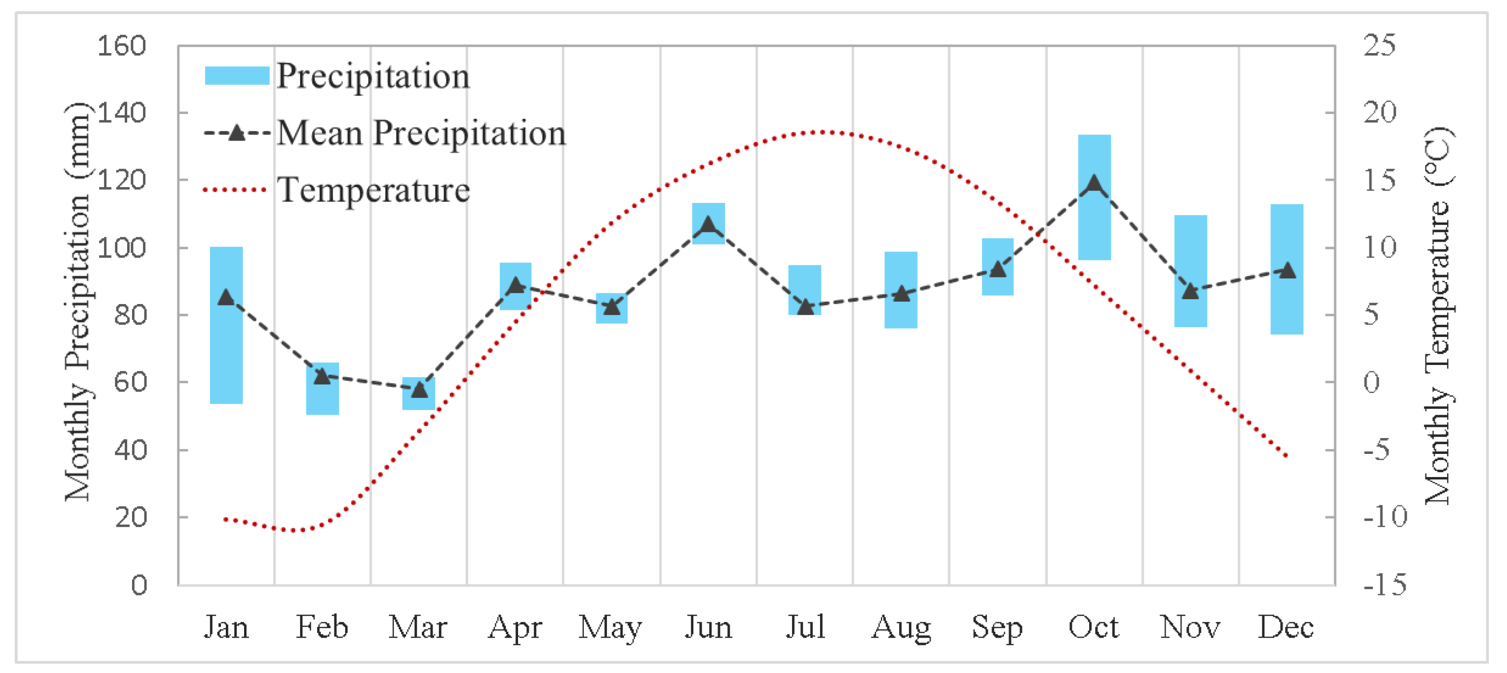
The Big East River (620 km2) and the Black River (1522 km2) watersheds, located in the northern part of Ontario, Canada, are chosen for the implementation of the proposed BMA scenario-based analysis (Figure 1). Both basins are mostly forested regions and their landscapes are moderately sloped with mean elevations of 450 and 300 meters above sea level for the Big East River and Black River watersheds, respectively. The historical daily streamflow data at the outlet of both watersheds (the only hydrometric station of each watershed) illustrate that high flows mostly occur in April when the snowmelt process plays an important role. Moreover, as can be seen from Figure 1, the only six available Environment Canada (EC) meteorological stations with reliable and sufficient historical data are located outside the boundaries of both watersheds. This represents an actual condition of watersheds with limited data availability. Analysis of the precipitation and temperature time-series of these six stations approximately shows the annual mean precipitation and the daily average temperature of 1050 mm and 5 °C, respectively. Moreover, the winter and summer average temperature are −9 °C and 18 °C, respectively, showing that all four seasons are defined clearly in both study areas (Figure 2).
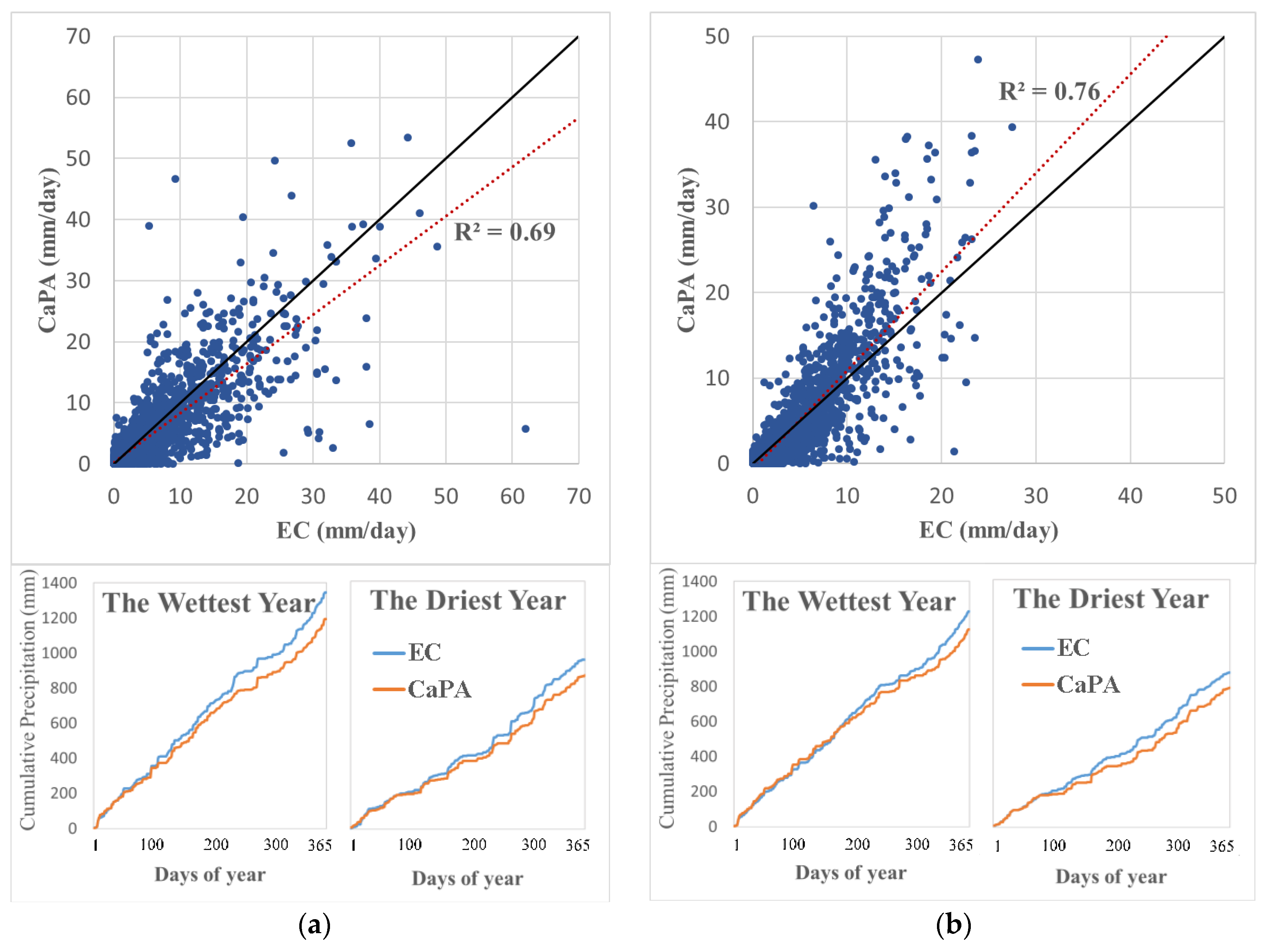
Besides the ground-based precipitation data, the archive of the daily aggregated form of the Canadian Precipitation Analysis (CaPA) was used as an alternative precipitation forcing input for hydrologic modeling of both watersheds. The CaPA is a gridded precipitation product with a spatial resolution of 15 km produced by the Meteorological Service of Canada based on the combination of various data sources, such as radar data, climate model data, and observations [46]. It was shown that the archived CaPA is a potential reliable source of precipitation for data-scarce regions [47]. In order to initially assess the precipitation variability of each basin using different datasets, primary analysis was performed. Two mean areal precipitation time-series for each watershed were derived from interpolated EC ground-based data using an inverse distance weighting method [48] and the CaPA data by applying a Thiessen polygon approach [49]. As can be seen from Figure 3, although CaPA provided more intense rainfalls specifically in the Black River watershed, it underestimated the amount of precipitation compared with the EC data in both watersheds. Moreover, the calculated daily correlation coefficients between EC- and CaPA-derived datasets (0.83 and 0.87 for the Big East River and Black River watersheds, respectively) show evidence of a linear relationship. However, by focusing on intense rainfall events (precipitation > 10 mm/day), the correlation coefficients were dramatically decreased to 0.42 and 0.48 for the Big East River and Black River watersheds, respectively. Therefore, there are remarkable differences between two datasets, especially at intense rainfall events, suggesting a significant amount of input uncertainty in poor-data watersheds. So, the authors used CaPA as a second forcing data for hydrologic models, which can help obtain a better quantification of the predictive uncertainty in the rainfall-runoff process using a Bayesian model averaging approach.
2.2. Standard Bayesian Model Averaging Technique
Bayesian model averaging is a statistical method for estimating probabilistic prediction based on various competing forecasts, possessing more reliability and accuracy than initial ensemble predictions. In this approach, the weighted averages of the individual forecasts’ probability distribution functions (PDFs) are used for generating the posterior distribution of forecasting variables. It was claimed through different studies that the higher weights are considered for better performing predictions in the training period [30,32,35,40,45].
Consider as a quantity which is going to be forecasted (i.e., predictand) and, therefore, denotes the training period of observation with data length . Having different models (i.e., ) results in , the ensemble of model predictions for the aforementioned training period, where . Based on the law of total probability and the assumption about the independence of different model forecasts, the PDF of the predictand conditioned on the models over the given training period can be formulated as follows [15]:
where is the posterior distribution of given the prediction of model and observed data , which simply can be considered as the forecast PDF of y based on model . Moreover, is the posterior probability or the likelihood of the model’s prediction being correct over the training period. Due to the assumption of models’ independency, the posterior probabilities of models should sum to unity, , and, consequently, they can be considered as weights (i.e., is the weight of model ). Furthermore, in the BMA approach, it is assumed that the model forecasts are unbiased, meaning that the expected value of the difference between observation and each model forecast should be equal to zero (i.e., for ). So, before BMA implementation, a bias-correction method should be used in order to create an unbiased ensemble of predictions. Although there are several bias-correction methods which all can be used for this aim, a linear-regression technique is utilized in the original BMA [16]. The bias-corrected results, (where and are the coefficients of the linear regression model), are replaced with the original model forecasts (). Therefore, the BMA predictive model (Equation (1)) can be rewritten as follows:
On the other hand, in the original BMA method, it is assumed that the aforementioned posterior probability (i.e., ) follows the normal (Gaussian) distribution, , with mean and variance , reflecting the uncertainty within the individual model . As explained in the introduction, some studies discussed that this assumption is a poor choice for a non-Gaussian forecast variable like streamflow. Therefore, they proposed implementing more representative distribution types (e.g., gamma distribution) or applying data transformation procedures (e.g., the Box–Cox transformation method [50]) for transforming data from their original space to a Gaussian space. It is worth mentioning that in the case of applying a data transformation procedure, the reverting process has to be able to apply in order to revert back to the original variable space.
Finally, based on Equation (2) and considering the Gaussian distribution, the BMA predictive mean and its associated variance can be determined using the two following equations [15,16]. The mean value is the weighted average of individual predictions, and the BMA variance consists of (1) between-model variance, reflecting the spread of the ensemble, and (2) within-model variance that represents the uncertainty regarding each model having the best forecast.
Successful implementation of the BMA method relies on the proper estimation of the parameters including weights () and variances () of each individual prediction (). Following Raftery et al. [16], in the standard BMA, the EM algorithm is utilized in order to maximize the log-likelihood function of the parameter vector () being approximated as follows:
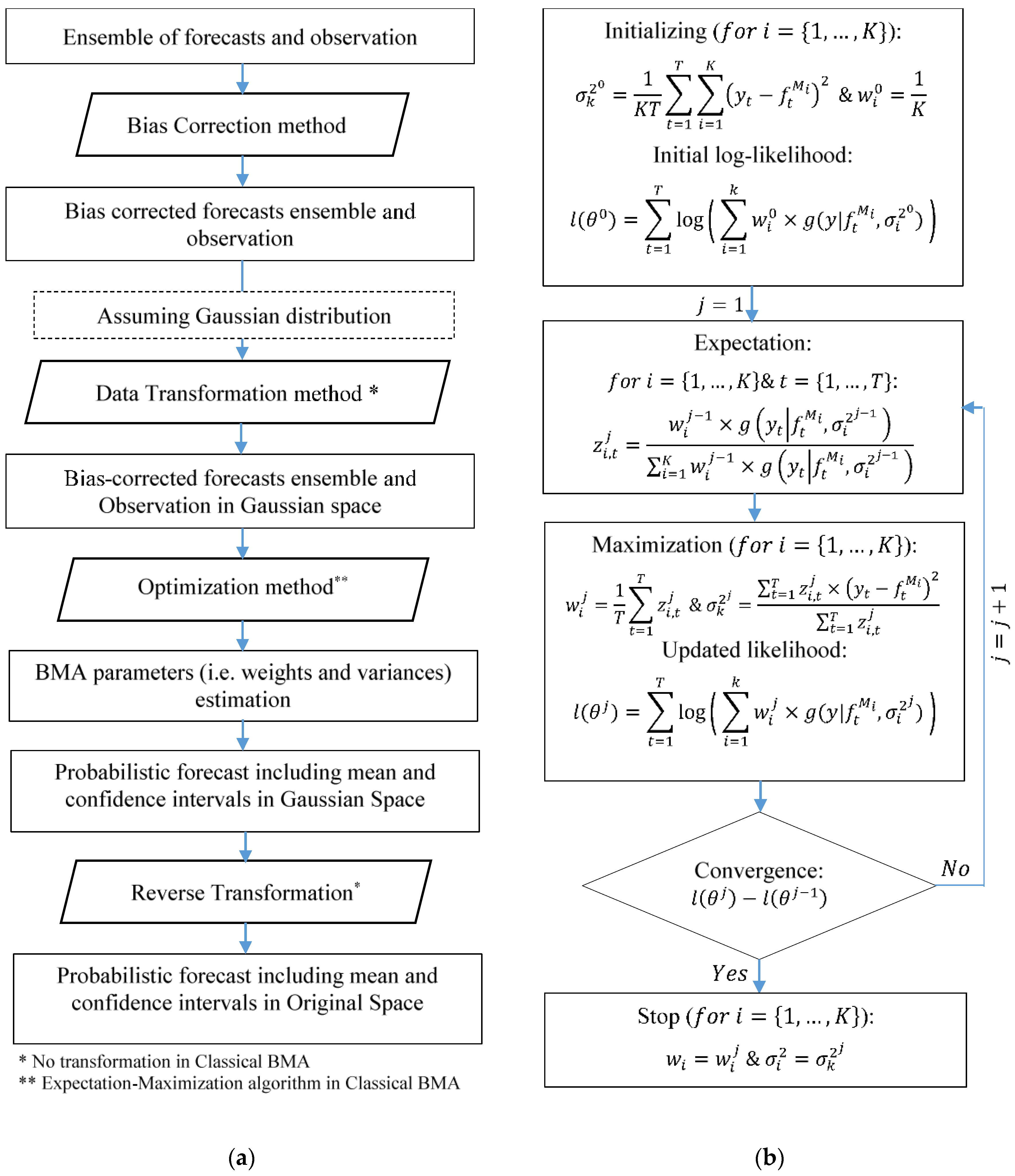
Given that there is no analytical solution for maximizing the summation of the aforementioned function over the training period, an iterative procedure such as the EM algorithm was used. In this procedure, the optimization problem was set by introducing a latent variable (). Apart initialization, this algorithm included an (1) expectation step, where the latent variable was calculated based on the current values of parameters, and a (2) maximization step, where the parameters were estimated according to the determined value of the latent variable (Figure 4b). It is worthy of note that, although the EM algorithm is computationally efficient, it is argued that using other optimization methods can lead to more robust estimation of the parameters.
According to the above equations, the flowchart of the classical BMA implementation is depicted in Figure 4a. As previously stated, some studies have been done in order to improve the reliability of the standard BMA approach by modifying some parts of the BMA structure. However, no comprehensive evaluation has been completed in order to clarify the effects of these modifications.
2.3. BMA Scenario-Based Analysis
In order to achieve the main goal of this research, we designed a BMA scenario-based analysis (Table 1) to see how the predictive streamflow simulation of the BMA approach was affected by modifying or changing some steps of the original BMA procedure. Implementation of the proposed evaluation allowed to assess how the accuracy and reliability of the BMA probabilistic results are sensitive to considering (1) different streamflow ensemble scenarios; (2) various data transformation methods; (3) more representative distribution types; (4) different standard deviation definitions; and (5) different optimization methods for parameter estimation. These scenarios are chosen in a way that cover most of the aforementioned modifications proposed by previous studies (explained in Section 1). Therefore, the effects of each modification or the combinations of modifications on BMA results can be assessed completely through the proposed analysis. The following paragraphs present a brief description of all aforementioned modification sections.
2.3.1. Streamflow Ensemble
As mentioned before, the ensemble can stem from different sources. Apart from considering different hydrologic models, various forcing precipitation inputs, as well as different reliable parameter sets of each rainfall-runoff model, can be considered for generating an ensemble of streamflow simulations. In this study, four different scenarios were determined to see how the BMA performance would change by considering a different number of ensemble members coming from various sources. In the first scenario, which was named “Multi-Model”, the ensemble was only based on different hydrologic models. In the two other scenarios (i.e., Multi-Model Multi-Input and Multi-Model Multi-Parameter), besides multiple hydrologic models, different precipitation datasets and various parameter sets were respectively utilized. Moreover, the last scenario was defined using all aforementioned sources (i.e., Multi-Model Multi-Input Multi-Parameter).
2.3.2. Data Transformation Methods
Four different data transformation procedures were assessed in the case of assuming normal function for the posterior distributions. The Box–Cox transformation method is a family of power transformations, and one of the common approaches is formulated as follows [50]:
and are the original and transformed data, respectively. is the Box–Cox coefficient and its common optimum value will be estimated using (1) observation data (i.e., Type 1) or (2) observation and simulations data (i.e., Type 2) by maximizing the log-likelihood function. Moreover, in the logarithmic transformation method, the daily streamflow data are transformed using natural logarithm in order to make them approximately follow the normal distribution. Another data transformation method evaluated in this study was the Empirical Normal Quantile Transformation (ENQT) procedure [51]. In this approach, the transformed data were calculated using the following equation, where is the inverse of the standard normal distribution and the empirical cumulative distribution of each value is denoted by .
It is of note that, instead of the empirical distribution, the generalized Pareto distribution is fitted to extrapolate the upper tail of the sample in the case of having a value which falls outside the range of the calibration data.
2.3.3. Distribution Types
Apart from using normal distribution, which is the main assumption of the original BMA method, the log-normal, gamma, and Weibull distributions are implemented as the conditional probability distribution function in Equation (2). These distributions are more representative for highly skewed data such as daily stream flows and may lead to better results.
2.3.4. Standard Deviation Types
In this study, following Vrugt [37], six various standard deviation parameterizations of the forecast distributions were assessed. The terms “common” and “individual” are used when all members of the ensembles have the same and distinct standard deviations, respectively. The other two terms illustrate if the standard deviations are dependent on the magnitude of the streamflow data (“non-constant”) or not (“constant”). Moreover, the last two types are defined by adding constant value in order to make the standard deviation be more than zero in all cases. The equations of all aforementioned standard deviation types and their corresponding number of parameters are presented in Table 2. In these equations, and , respectively, denote the standard deviation and the daily discharge of the th simulated streamflow at time-step . Also, is the total number of members in the ensemble.
2.3.5. Optimization Methods
Given the criticism of the EM algorithm regarding its ability to achieve the global optimum estimation and its lack of flexibility in applying to the various aforementioned modifications, the dynamically dimensioned search (DDS) method [52] was used as the alternative optimization technique for estimating the BMA parameters. Dynamically dimensioned search is a single global optimization method which finds the optimal solution by dynamically rescaling the search space dimension. Similar to the EM algorithm, the log-likelihood of the BMA parameter vector is considered as the objective function in the DDS optimization approach. Correspondingly, the DDS parameter estimations can be utilized as benchmarks for evaluating the application of the EM algorithm.
2.4. Hydrological Models
Using different hydrologic models for generating an ensemble of competing simulated stream flows is the main basis of the BMA approach [9]. As listed in Table 3, the seven different rainfall-runoff models implemented in this study are SAC-SMA, MAC-HBV, SMARG, GR4J, and three HEC-HMS [53] based models. There are different methods available for each part of the hydrologic cycle in the HEC-HMS platform. In this study, we used the rational combination of loss (i.e., deficit and constant, and soil moisture accounting) and baseflow (i.e., recession and linear reservoir) methods for generating the HEC-HMS-based models with different structures. In the HEC-HMS type 1 and 2, the recession baseflow method is implemented with the deficit and constant and soil moisture accounting loss approaches, respectively, while HEC-HMS type 3 is developed using the combination of the soil moisture accounting and linear reservoir methods.
All of the aforementioned models are lumped conceptual ones, which have been shown to provide comparable or even better performance in comparison to the more complex models (e.g., distributed models) in data-poor watersheds [54,55,56]. Moreover, by adding the simplified Thornwaite formula [57,58] to the first four models and feeding HEC-HMS models the average monthly potential evapotranspiration calculated using Hargreaves equation [59], the only inputs to all models are the mean areal daily precipitation and temperature. Also, streamflow estimation at the outlet of the watershed is the only output of these models. It is worth mentioning that due to the importance of the snow accumulation and melt process in cold regions, three different snowmelt modules are implemented with different hydrologic models. The available temperature-index method in the HEC-HMS software [53] was used for the three aforementioned HEC-HMS-based models. The simple degree-day snowmelt module (DDM) [58] was added to the SMARG and GR4J models, while the SACSMA and MACHBV models were combined with the more complex SNOW17 snowmelt estimation method [60,61] for snow–rainfall discrimination and quantifying snowpack changes over the simulation period.
On the one hand, in the DDM approach, the snowmelt is calculated using a linear relationship between snowmelt and air temperature, where a constant melt rate factor is considered. However, the antecedent temperature index is used for melt-rate determination in the HEC-HMS snowmelt approach [62]. On the other hand, the SNOW17 is a process-based temperature-index method that considers different physical processes in the snowmelt procedure such as energy exchange between air and snow, heat storage and deficit of the snowpack, liquid water storage, etc. Also, upper and lower preset temperature thresholds are used for distinguishing between rainfall and snowfall in both the DDM and SNOW17 models [63]. For a more detailed description of all snow routines, the readers are referred to the aforementioned citations.
Furthermore, five different objective functions, including Nash–Sutcliffe efficiency (NSE) [68], Kling–Gupta efficiency (KGE) [69], Nash volume error (NVE) [58], peak-weighted root mean square error (PWRMSE) [70], and modified Nash volume error (MNVE) were used through the dynamically dimensioned search (DDS) algorithm for finding the optimized parameter sets of each individual model. The latter objective function was defined in order to greatly focus on high flows by using the NSE based on square of discharge ():
where volume error () is:
and based on square of discharge () is calculated as follows:
In the above equations, and are the observed and simulated streamflow, respectively, while is the data length. The years 2006 to 2011 were considered the calibration period and the validation was carried out for the 2012–2015 (4 years) period. It is of note that the best performing parameter set of each individual model, determined based on validation results, is utilized for generating multi-model and multi-model multi-input ensemble scenarios. For a detailed description of the aforementioned hydrologic models and objective functions, the readers are referred to the cited references.
2.5. Performance Evaluation Metrics
Five model evaluation statistics are used for comparing the accuracy, reliability, and sharpness of the results of different BMA variants. The accuracy is defined as the error between deterministic simulations and their corresponding observations. In this study, besides the well-known Nash–Sutcliffe efficiency criteria, being calculated according to squared (; Equation (10)) and logarithmic (; Equation (11)) transformed streamflow data, were the two other deterministic performance criteria being, respectively, focused on the accuracy of the high- and low-flow simulations.
is the observed variable and represents the simulated variable which is considered to be the expected value of the BMA predictive simulation. Also, is the length of the dataset. All -based criteria vary between −∞ and 1 with the best value of 1.
Furthermore, two other probabilistic performance measurements proposed by Xiong et al. [71] were adopted for quantitative evaluation of the BMA probabilistic results. The containing ratio () is defined as the percentage of the observed data which falls within the 95% confidence interval, and the average bandwidth () is the average width of the corresponding bound. The former measures the reliability while the latter is used for quantifying the sharpness of the results. Given two forecasts with the same (i.e., same reliability), the one with a smaller shows a greater precision.
In the above equations, the number of observations being contained in the 95% confidence interval is denoted by and , respectively, show the upper and lower boundaries of the 95% confidence interval at time-step . In addition, for evaluating the probabilistic performance of different BMA variants regarding high flows, we calculated the two aforementioned probabilistic indices using the streamflow values of more than 90 percentiles (denoted by and for the containing ratio and the average bandwidth, respectively).
3. Results and Discussion
3.1. Choosing the Best Ensemble Scenario
One of the vague points of the BMA approach in the literature is the optimal number of members of the ensemble and how they should be generated. The prime step before employing any BMA variants is constructing the most reliable ensemble, which provides the best results. Therefore, as the first section of the proposed analysis, the four aforementioned scenarios of different streamflow simulation ensembles were used in the original BMA for both the Big East River and Black River watersheds, and a comparison was made among their results (Table 4). Given the two different input scenarios and five various parameter sets for each hydrologic model, there were 7, 14, 35, and 70 simulated stream flows for the Multi-Model (M-M), Multi-Model Multi-Input (M-MI), Multi-Model Multi-Parameter (M-MP), and Multi-Model Multi-Input Multi-Parameter (M-MIP) ensemble scenarios, respectively.
If the BMA performance based on the Multi-Model (M-M) ensemble scenario is considered as the benchmark, there was no significant improvement when the performance statistics focusing on the whole and low discharges were considered. However, by focusing on the high flow-based criteria, the results show that considering the forcing precipitation as another source of uncertainty besides hydrologic models enhanced both the deterministic and probabilistic BMA results. This improvement was more significant in the Black River watershed, where the accuracy and reliability of the BMA using the M-MI scenario increased by about 10 and 25 percent based on the and criteria, respectively. It is worth mentioning that, all seven additional members of the streamflow simulations (generated by considering CaPA as forcing inputs of each individual model) being used in M-MI compared to M-M, possessed lower individual deterministic predictive skills than existing models in both ensemble scenarios.
Moreover, surprisingly, although the Multi-Model Multi-Parameter ensemble scenario included all members being utilized in the benchmark scenario, the overall performances of the BMA method implementing them slightly deteriorated in both watersheds. This may be due to the main initial assumption of the BMA methodology, where the law of total probability needs not only collectively exhaustive but also independent members of the ensemble. Furthermore, using 70 members in a streamflow ensemble (constructed by considering all aforementioned sources) enhanced the probabilistic performance of the BMA, specifically in high flows, while its performance was not as reliable and sharp as in the case where the M-MI scenario was applied.
Altogether, it can be concluded that the M-MI ensemble scenario was the most appropriate one, providing better probabilistic and deterministic results. Accordingly, for the rest of the application of the proposed analysis, the Multi-Model Multi-Input ensemble scenario, including 14 members of streamflow simulations, was implemented for both watersheds. As a result, 48 probabilistic streamflow simulations were generated considering the combination of the different modifications, including distribution, standard deviation, and data transformation methods (Table 1). The parameters for all 48 BMA variants were calibrated using the DDS optimization method for the period from 2006 to 2011, considering one year as a warm-up period, and the years 2012 to 2015 were considered for validation.
3.2. BMA Weights Versus Models’ Performance Statistics
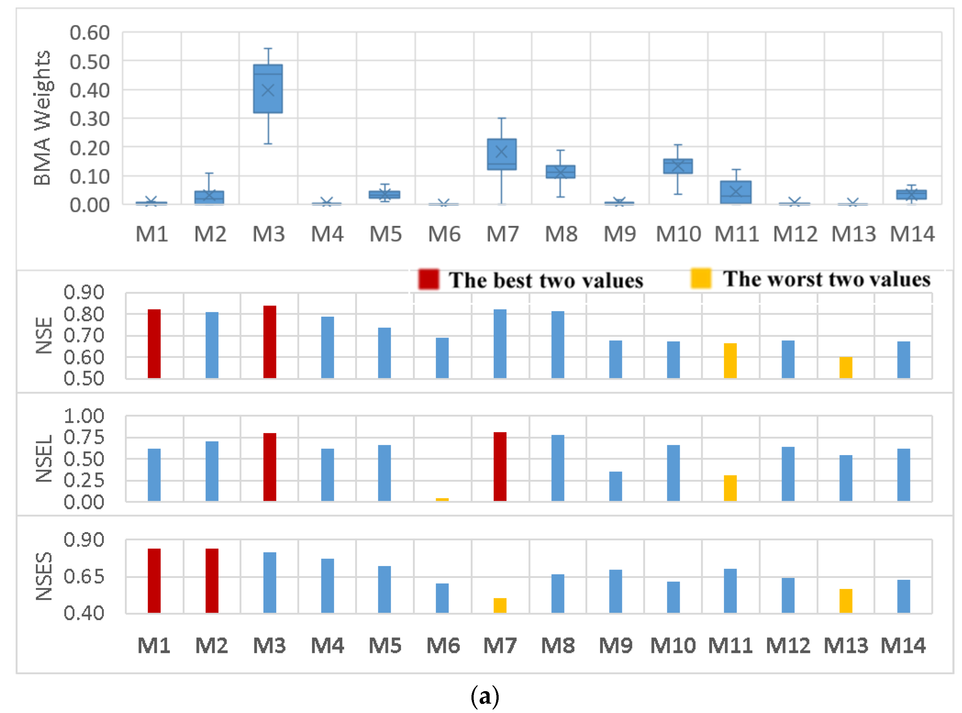
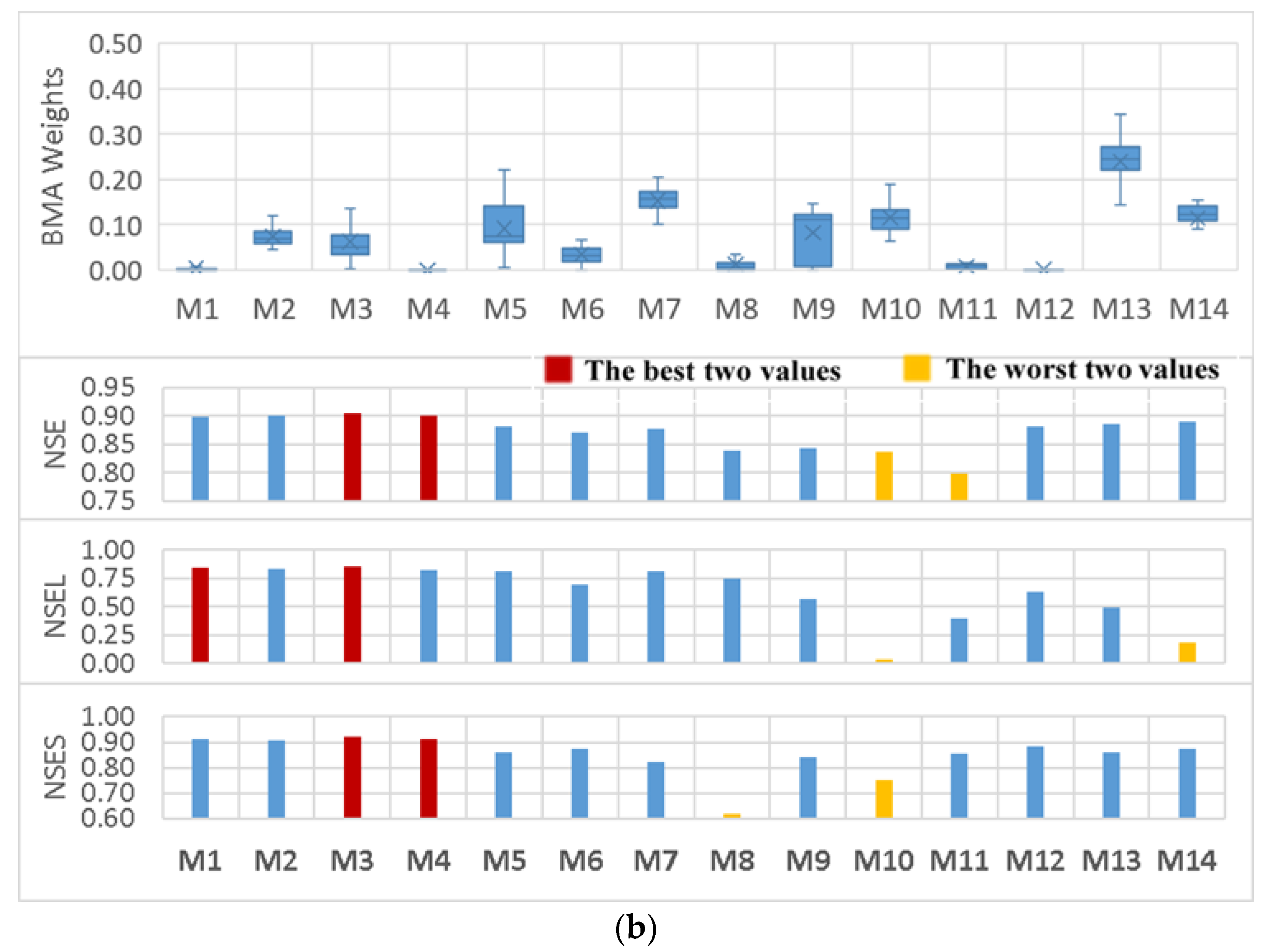
In the first place, besides assessing the effects of various modifications, a comparison was made between the BMA weights of different members of the ensemble and the performance of the corresponding models during the calibration period for both the Big East River and Black River watersheds (Figure 5).
Interestingly, it can be seen that the distributions of the weights amongst different members do not properly agree with the previous belief, where the weights reflect the models’ performance. For instance, in the Big East River watershed, although M1 was one of the most promising simulations comparing different performance statistics, its weights were not predominant compared to other BMA variants. In addition, in the Black River watershed, M10 had relatively high weights, while its performance was not good in comparison to the other models. Similarly, the first four members of the ensemble (i.e., M1 to M4) possessed the most reliable deterministic results, although they received relatively low weights.
Moreover, closer inspection of the graphs (in Figure 5) shows that low flows played an important role in the determination of the BMA weights, specifically in the Big East River watershed where the specified weights relatively fit with the performance statistics. This may be justifiable by the fact that more than 90 percent of the daily streamflow observations were less than 25 m3/s while this fraction was around 60 for the Black River watershed (Figure 6).
3.3. The Effects of Different Modifications
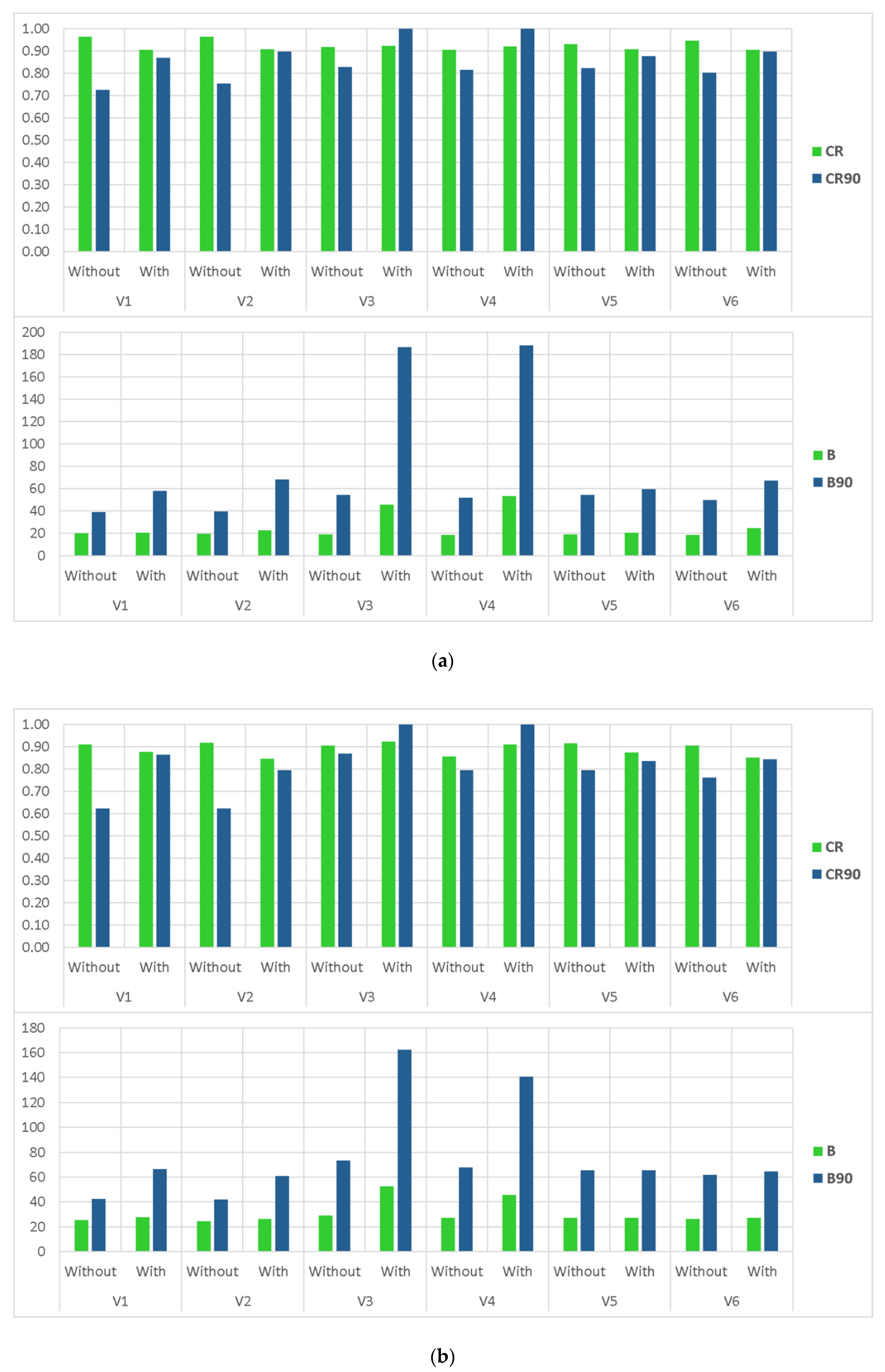
The evaluations of various BMA modifications (i.e., different distribution and standard deviation types, and data transformation methods) will be provided in this section. As discussed previously, one recommended solution in order to enhance the performance of the original BMA approach is using data transformation procedures for generating approximately normally distributed data. Figure 7 compares the accuracy and reliability of the BMA variants with and without application of data transformation procedures. It can be recognized that, in general, the BMA deterministic performance did not change significantly by applying data transformation methods. On the other hand, although the data transformation caused a remarkable enhancement of the BMA’s reliability in high flows, the sharpness of the results was largely reduced.
Further analysis (Figure 8) shows that the influence of applying data transformation modification on the BMA performance is highly related to the types of standard deviation being implemented in the procedure. In the case of considering common and individual non-constant variance types (i.e., V3 and V4, respectively), implementation of a data transformation method leads to under confident and negatively biased probabilistic results. It is much more recognizable in high flows where the containing ratios of the 95% confidence interval are around one, while their corresponding bandwidths increase largely. However, for other types of standard deviations where a constant value can play an important role, the reliability of the high flows’ simulation is partly improved without a drastic drop in their sharpness.
Moreover, Table 5 represents the performance criteria of different BMA variants, being developed using normal distribution and variance types V5 and V4, to compare different data transformation procedures. Based on the results, the only data transformation procedure providing acceptable probabilistic results with the use of heteroscedastic standard deviation without a constant value (i.e., V3 and V4) was the empirical normal quantile transform (i.e., T4) method. However, in general, by looking at the BMA variants based on variance type V5, as a representative of the other standard deviation forms, none of the methods appeared superior to the others, indicating that changing the data transformation approaches had little impact on BMA model performance.
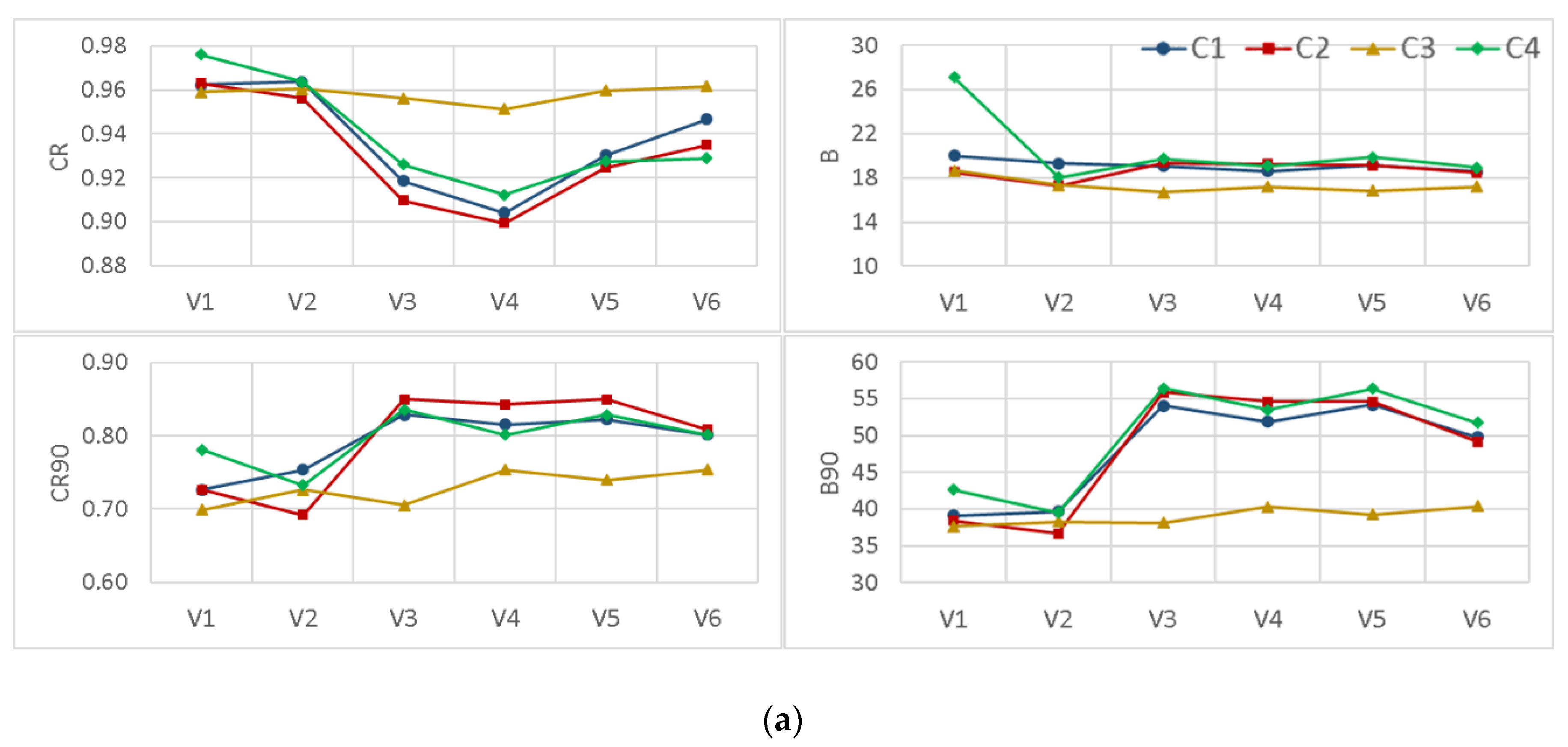
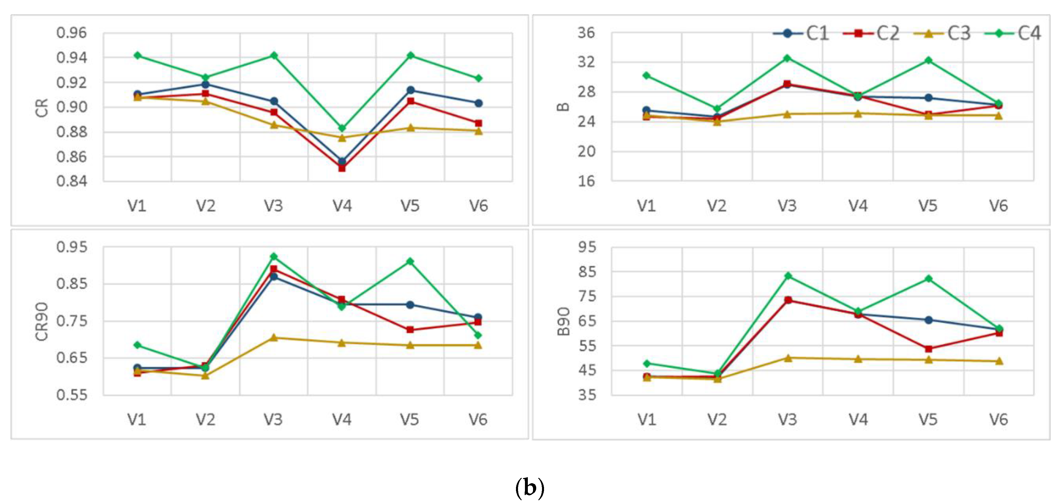
Besides using data transformation procedures, the two other BMA modifications evaluated in this study were considering other distribution types and implementing various standard deviation forms (Figure 9). The comparison between the applications of four different distribution functions proposed in the scenario-based analysis shows that, in general, the implementation of the log-normal distribution (i.e., C3) enhances the reliability and sharpness of the BMA results simultaneously. However, it underestimates when considering high flows, which is not appropriate in most operational hydrologic fields such as flood forecasting. As can be seen from the figure, in the case of using a common constant standard deviation type (i.e., V1), even though the coverage of the 95% confidence interval slightly increased by applying the Weibull distribution, the model lost its sharpness by leading to a higher bandwidth in both watersheds. Moreover, by assessing the effects of using different standard deviation types, it is apparent that considering “non-constant” types leads to more reliable results especially for high flows. However, using “individual” variance types does not affect the BMA performance in comparison to their corresponding “common” ones.
Taken together, these results suggest that changing the distribution type of the BMA posterior probability from normal to more representative ones does not enhance the BMA probabilistic performance, significantly. However, implementation of “non-constant” standard deviation types improved the BMA predictive results specifically regarding high flows.
3.4. Expectation-Maximization Algorithm Versus Dynamically Dimensioned Search Method
The EM algorithm was implemented in the classical BMA method, which is criticized for not being able to reach global optimum estimations. Here, as a part of the evaluation, six different BMA variants were calibrated using the EM algorithm, and a comparison was made with the corresponding DDS-based calibrated models. The results, as shown in Figure 10, indicate that the differences among estimated BMA weights using EM and DDS methods were negligible, and both methods led to the approximately similar optimal solution.
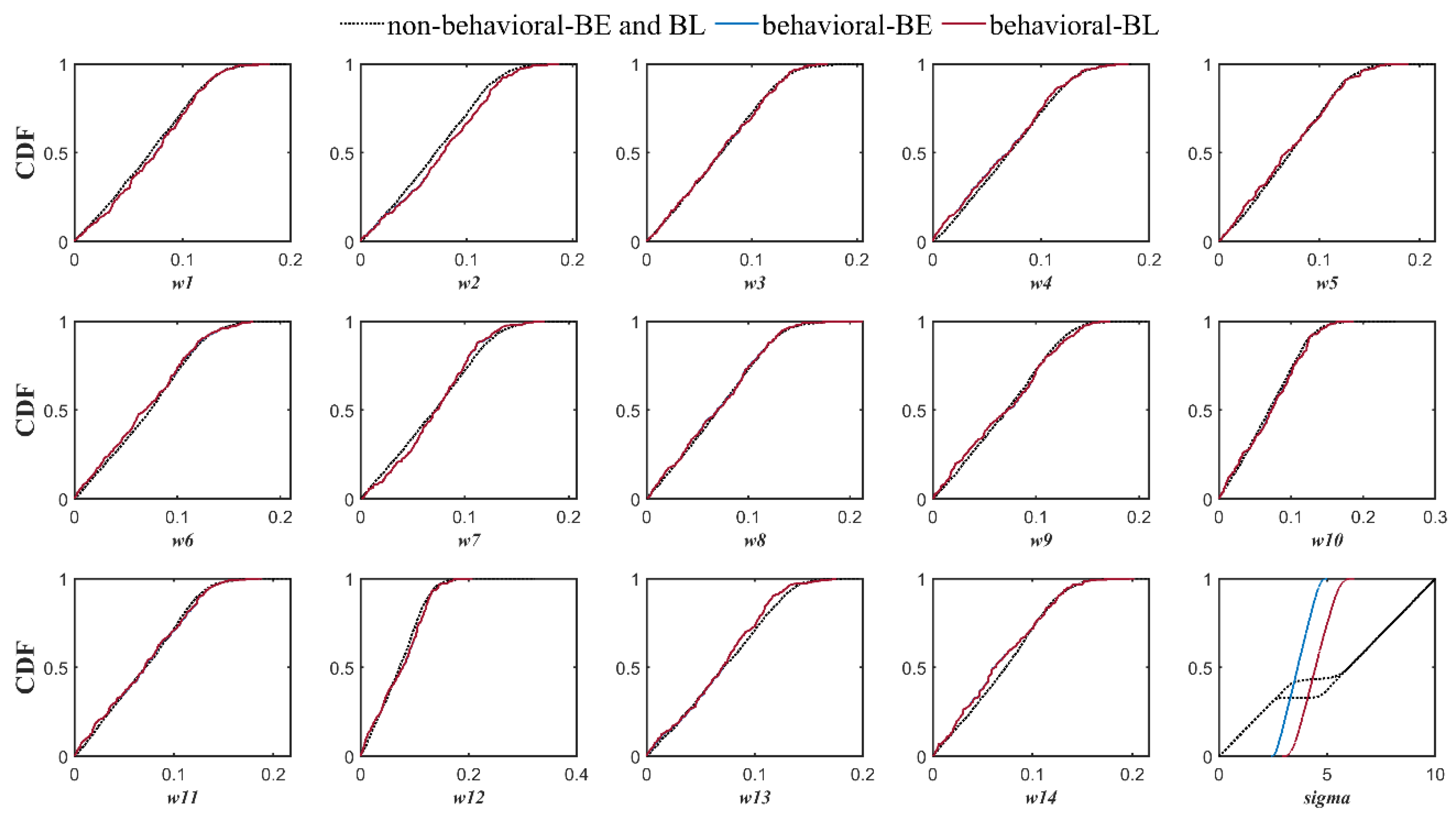
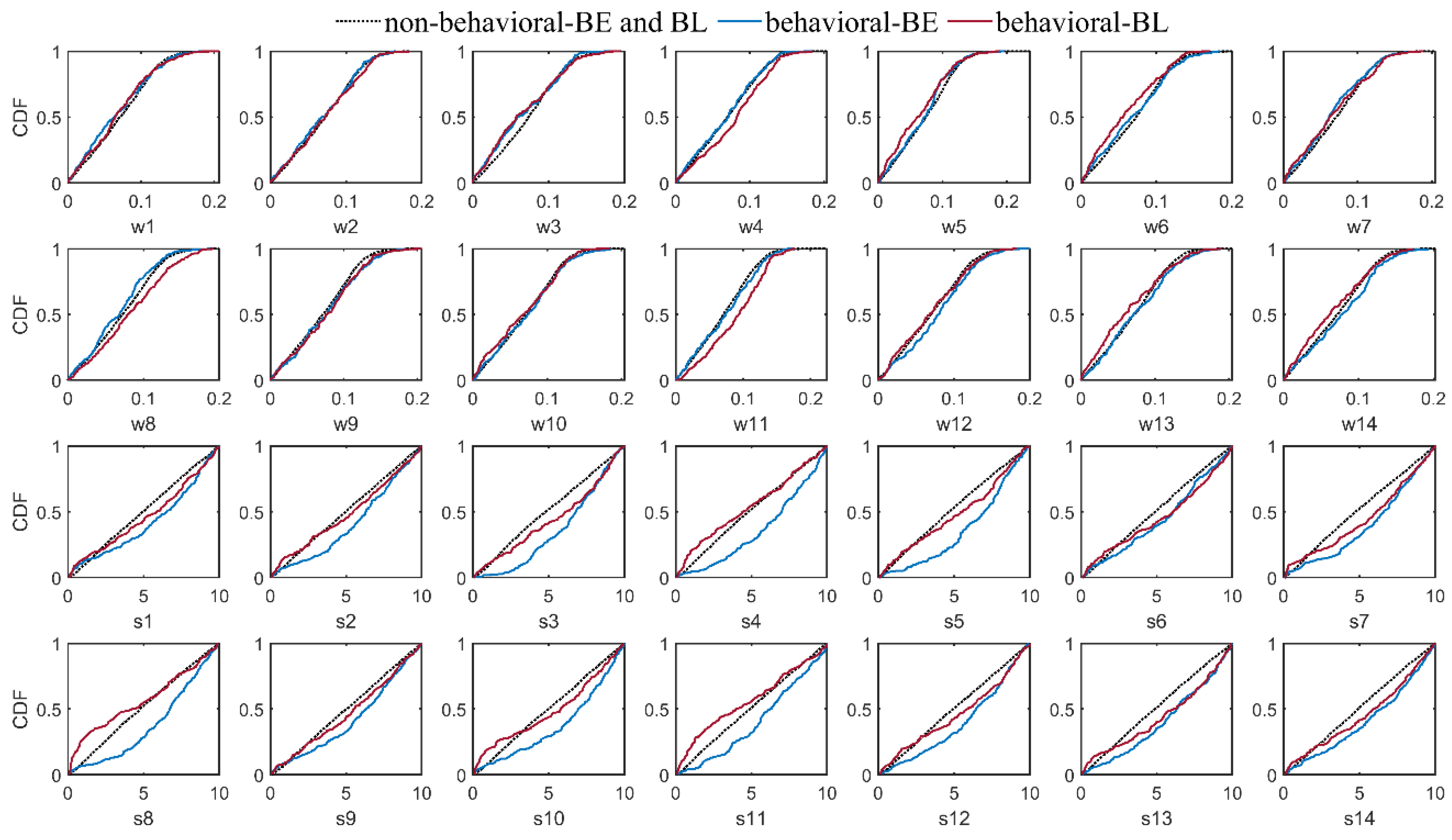
To specify the logic behind these results, the authors applied the regional sensitivity analysis (RSA) method [72] to original BMA with “common” (Figure 11) and “individual” (Figure 12) constant standard deviation types (i.e., C1V1T0 and C1V2T0 BMA variants, respectively). In this method, the Monte Carlo simulation technique is used for generating various parameter sample sets, and then, the samples are divided into two behavioral and non-behavioral ones based on a predefined threshold. So, qualitative comparison of the empirical cumulative distribution functions (CDFs) of the behavioral and non-behavioral parameter sets illustrate the most sensitive parameter(s). The RSA results for both the Big East River and Black River watersheds reveal that the objective function is significantly sensitive to standard deviation values, while the models’ weights can be considered non-sensitive parameters.
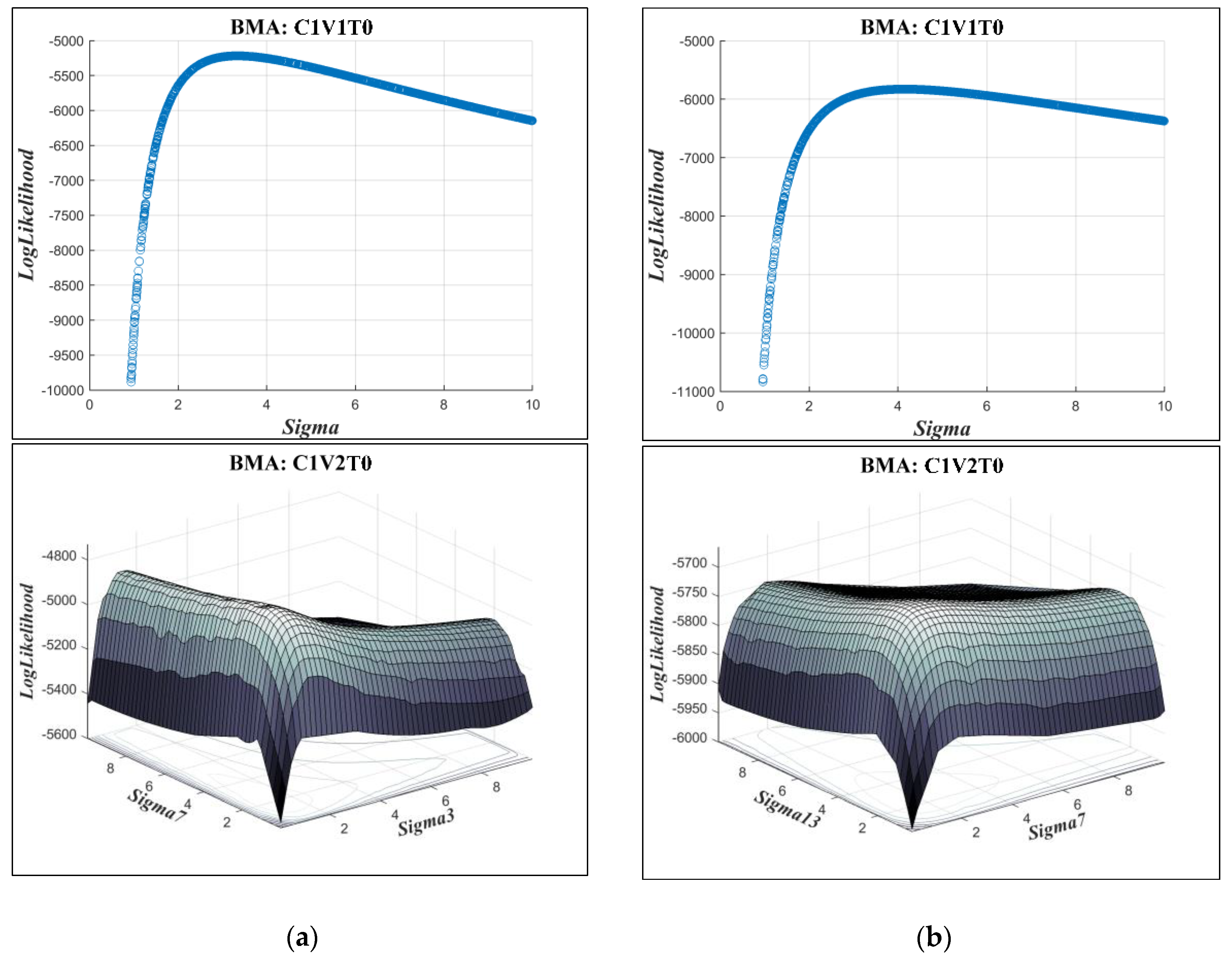
Therefore, the variation of the log-likelihood function is evaluated by changing the most sensitive parameters (standard deviations) between their lower and upper bounds while the other parameters are constant and equal to their nominal values (i.e., the calibrated values). The results, illustrated in Figure 13, show that in all evaluated cases, the negative log-likelihood, which is the objective function for both optimization processes, is a convex function so that a local optimization method such as the EM algorithm can lead to global optimal estimation of parameters. Consequently, although the EM algorithm is considered a local optimization method, it can estimate the original BMA parameters like other global optimization techniques. It is of note that the original EM method can only be applied for the constant variance types and it requires modifications if other distribution or standard deviation types need to be incorporated. However, DDS or any other global optimization techniques can be used by different BMA modifications without any difficulty.
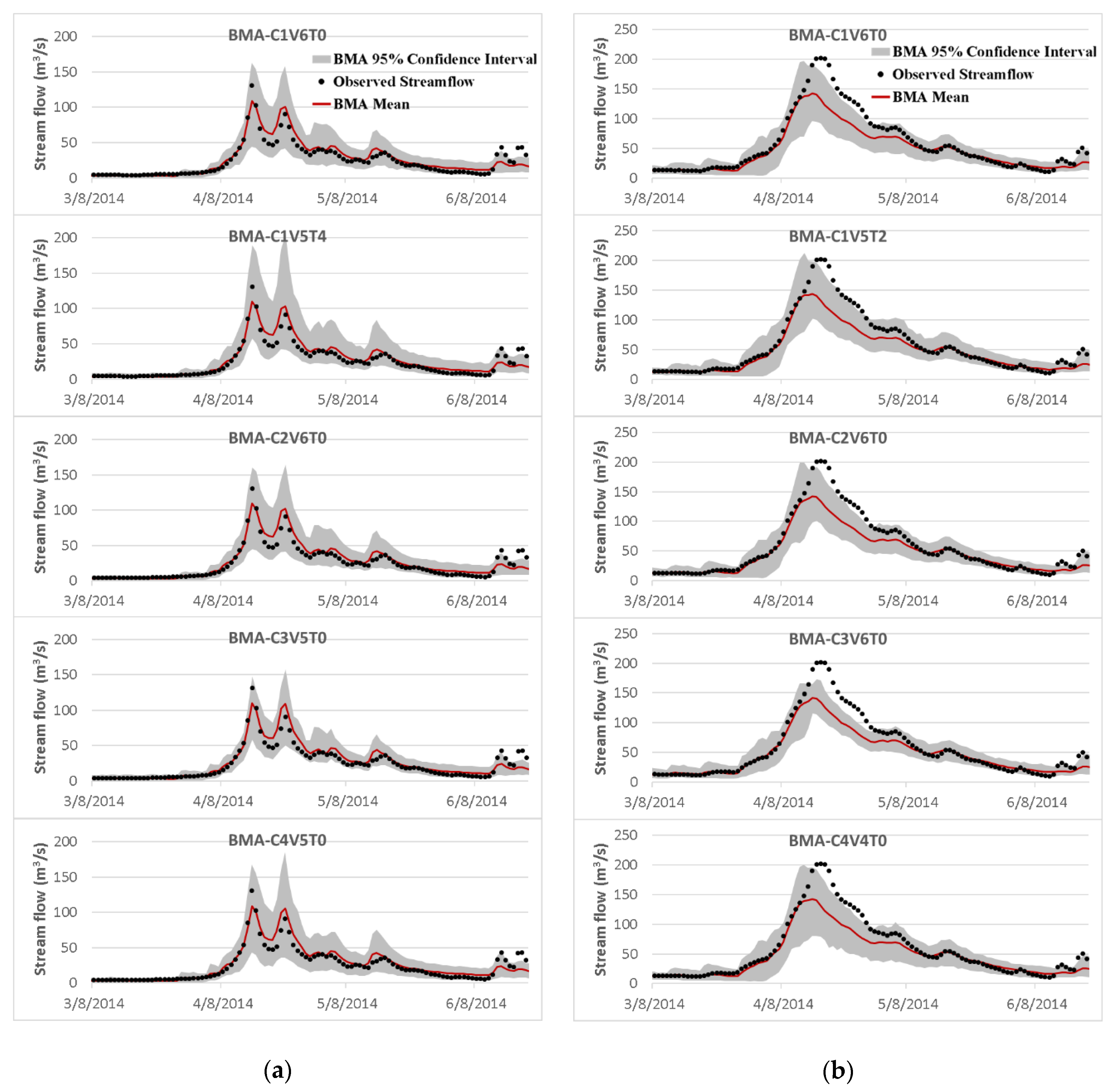
Finally, in order to complete the evaluation and find the most promising types of BMA modifications, the best combinations were selected for each distribution type and their performances during the validation period were compared with each other (Table 6). Additionally, for qualitative inspection of the best models, Figure 14 illustrates the mean and the 95% predictive bounds of the BMA streamflow simulations for a representative portion of the validation period. What stands out in Table 6 is that the standard deviation types in all the best-selected BMA models were the non-constant ones, and most of them were the heteroscedastic variance with a constant value (i.e., V5 and V6). Moreover, as expected based on the previous comparison, although the best BMA modification with data transformation procedure provided higher reliability, the sharpness of the results partially deteriorated in high flows in both watersheds. Also, it can be seen that the best BMA model using the log-normal distribution type underestimated high flows significantly, while its other performance statistics showed almost the same predictive performance in comparison to the other best models. It is worthy of note that there was no significant difference among the accuracy of the various best-selected BMA variants.
Furthermore, as it was concluded beforehand, there was not a significant difference among the predictive performances of the different BMA variants utilizing various distribution types. However, the implementation of the gamma distribution type seemed to provide more balanced and consistent results in comparison to the other ones in this case. It is of note that even by comparing the most promising models, which possessed approximately similar performances, the calibrated weights showed some changes confirming that there were no specific BMA weight combinations that led to the best results (Figure 15).
4. Summary and Conclusions
This study provides the first assessment of the previously proposed modifications for the original BMA methodology and documents how they affect the probabilistic and deterministic performance of the BMA-derived results for daily streamflow simulation. A scenario-based analysis was designed where the application of four diverse streamflow ensemble scenarios, different data transformation procedures, various distribution types, six different types of standard deviation, and two optimization algorithms were assessed thoroughly.
The summary of the obtained results from applying the proposed evaluation into two data-poor watersheds is as follows:
- Comparing different ensemble scenarios indicated that, besides using multi-models, considering various forcing precipitation scenarios in generating members of an ensemble leads to better probabilistic and deterministic results in data scarce regions, where the estimation of mean areal precipitation always comes with noticeable errors. However, not only using a multi-model multi-parameter scenario did not provide better results, it also slightly reduced the reliability of the BMA simulations.
- In contrast to earlier findings, however, the results showed that the BMA weights were not completely in accordance with individual model performance. There were some highly weighted hydrologic models with relatively lower performance in comparison to the others in both watersheds. In addition, various BMA modifications led to different combinations of weights and all had almost the same predictive power.
- Applying data transformation generally yielded an improvement in the reliability of the BMA results. However, except for the empirical normal quantile approach, using other data transformation methods concurrent with implementing non-constant standard deviation without a constant parameter dramatically deteriorated the sharpness of the results, specifically in high flows.
- Incorporation of the more representative distribution types did not show a particular superiority over the classic BMA method, where the posterior predictive distributions were assumed to be Gaussian. However, implementing non-constant standard deviations enhanced the predictive capability of the BMA model, especially for high flows that are often of particular attention in operational hydrology.
- The expectation-maximization algorithm provided almost the same results as the dynamically dimensioned search (DSS) method, which showed its ability to estimate BMA parameters well enough. However, the only drawback was that it could not easily be applied for all BMA variants when the distribution or standard deviation types were changed.
In general, the findings of this study suggest that the simulation skill of individual members are less important than how the whole ensemble captures the variability of the observation without overlapping. In other words, using ensemble members with diverse simulation skills can enhance the quality of the BMA results, while simply increasing the number of members in the ensemble does not always lead to better results. Although possessing high-performance models is necessary for obtaining reliable results, there is some information that is only provided by the relatively lower performing models and, consequently, considering them as members of the ensemble can enhance the BMA’s predictive performance. The notable BMA weights of some of these models are another convincing justification for this conclusion. In addition, it was shown that in regions where the network of meteorological stations was sparse, using other sources of precipitation data, such as archived radar- or satellite-based products as inputs into the hydrologic models, can lead to a more exhaustive streamflow ensemble that enhances the BMA’s performance.
Moreover, another implication of these results is that the most effective BMA modification in the positive direction (i.e., enhancing the predictive performance) is the implementation of non-constant standard deviation. Increasing the variance of errors in line with flow level seems to be more realistic and enhances the reliability of the BMA results significantly for high flows (an average of 20% improvement in the reliability of high-flow simulations in both the Big East River and Black River watersheds over the whole period). However, considering the more representative distribution types does not highly affect the BMA-derived probabilistic and deterministic results. Moreover, although using data transformation procedures enhanced the reliability of the results, even more than applying non-constant variance, it can lead to a notable wide confidence interval width in high flows. Therefore, much more attention must be paid to the sharpness of the high-flow probabilistic simulation in the case of implementing data transformation. Furthermore, the results showed the robustness of the EM algorithm for estimating the original BMA parameters, while it was not easily applicable to all BMA modifications. Thus, applying a global optimization method is recommended in the case of using various BMA variants.
Although the two watersheds in this study share approximately the same land use and climatology, their hydrologic responses are not quite similar and lead to two different empirical CDFs of streamflow data. Therefore, it can be said that the aforementioned conclusions about the effects of different modifications on BMA results can be considered as useful recommendations in future studies. However, in order to provide more comprehensive conclusions, it is worth applying the proposed BMA modifications analysis in watersheds with very different topography and climatology (e.g., mountainous or coastal areas and tropical or semi-arid regions) in future studies. Furthermore, although possessing mutually exclusive and collectively exhaustive ensemble members is one of the main assumptions of the BMA method, no studies have tried to overcome this issue. Although this study assessed the effects of various ensemble scenarios on BMA performance and provided fresh insight into the importance of establishing an ensemble with the aforementioned properties, there has not been a specific method about how these members should be generated and selected. Consequently, further studies need to be carried out to establish new ideas for solving this remaining challenge.
Author Contributions
Conceptualization, P.D. and P.C.; Data curation, P.D.; Formal analysis, P.D.; Investigation, P.D.; Methodology, P.D. and P.C.; Software, P.D. and P.C.; Supervision, P.C.; Validation, P.D. and P.C.; Visualization, P.C.; Writing—original draft, P.D.; Writing—review and editing, P.C.
Funding
This work was funded by the Natural Sciences and Engineering Research Council of Canada under Canadian FloodNet project (Grant number: NETGP 451456).
Acknowledgments
We would like to thank the Ministry of Natural Resources and Forestry, Surface Water Monitoring Center for providing some of the study data and Tara Razavi for providing Matlab source codes for the MACHBV, SACSMA, and Snow17 models.
Conflicts of Interest
The authors declare no conflict of interest.
References
- Chen, X.; Yang, T.; Wang, X.; Xu, C.Y.; Yu, Z. Uncertainty intercomparison of different hydrological models in simulating extreme flows. Water Resour. Manag. 2013, 27, 1393–1409. [Google Scholar] [CrossRef]
- Liu, Z.; Guo, S.; Zhang, H.; Liu, D.; Yang, G. Comparative study of three updating procedures for real-time flood forecasting. Water Resour. Manag. 2016, 30, 2111–2126. [Google Scholar] [CrossRef]
- Moradkhani, H.; Sorooshian, S. General review of rainfall-runoff modeling: Model calibration, data assimilation, and uncertainty analysis. In Hydrological Modelling and the Water Cycle: Coupling the Atmospheric and Hydrological Models; Sorooshian, S., Hsu, K.L., Coppola, E., Tomassetti, B., Verdecchia, M., Visconti, G., Eds.; Springer: Berlin/Heidelberg, Germany, 2008; Volume 63, pp. 1–24. ISBN 978-3-540-77843-1. [Google Scholar]
- Shrestha, D.L. Uncertainty Analysis in Rainfall-Runoff Modelling—Application of Machine Learning Techniques: UNESCO-IHE. PhD Thesis, IHE Delft Institute for Water Education, Delft, The Netherlands, 2009. [Google Scholar]
- Madadgar, S.; Moradkhani, H. Improved bayesian multimodeling: Integration of copulas and bayesian model averaging. Water Resour. Res. 2014, 50, 9586–9603. [Google Scholar] [CrossRef]
- Michaels, S. Probabilistic forecasting and the reshaping of flood risk management. J. Nat. Resour. Policy Res. 2015, 7, 41–51. [Google Scholar] [CrossRef]
- Seo, D.J.; Herr, H.D.; Schaake, J.C. A statistical post-processor for accounting of hydrologic uncertainty in short-range ensemble streamflow prediction. Hydrol. Earth Syst. Sci. Discuss. 2006, 3, 1987–2035. [Google Scholar] [CrossRef]
- Georgakakos, K.P.; Seo, D.J.; Gupta, H.; Schaake, J.; Butts, M.B. Towards the characterization of streamflow simulation uncertainty through multimodel ensembles. J. Hydrol. 2004, 298, 222–241. [Google Scholar] [CrossRef]
- Vrugt, J.A.; Robinson, B.A. Treatment of uncertainty using ensemble methods: Comparison of sequential data assimilation and Bayesian model averaging. Water Resour. Res. 2007, 4. [Google Scholar] [CrossRef]
- Granger, C.W.; Ramanathan, R. Improved methods of combining forecasts. J. Forecast. Pre-1986 Chichester 1984, 3, 197–204. [Google Scholar] [CrossRef]
- Shamseldin, A.Y.; O’Connor, K.M. A real-time combination method for the outputs of different rainfall-runoff models. Hydrol. Sci. J. 1999, 44, 895–912. [Google Scholar] [CrossRef]
- Shamseldin, A.Y.; O’Connor, K.M.; Liang, G.C. Methods for combining the outputs of different rainfall–runoff models. J. Hydrol. 1997, 197, 203–229. [Google Scholar] [CrossRef]
- Hoeting, J.A.; Madigan, D.; Raftery, A.E.; Volinsky, C.T. Bayesian model averaging: A tutorial. Stat. Sci. 1999, 14, 382–401. [Google Scholar]
- Raftery, A.E. Bayesian model selection in structural equation models. In Testing Structural Equation Models; SAGE: Thousand Oaks, CA, USA, 1993; Volume 154, pp. 163–180. [Google Scholar]
- Raftery, A.E.; Madigan, D.; Hoeting, J.A. Bayesian model averaging for linear regression models. J. Am. Stat. Assoc. 1997, 92, 179–191. [Google Scholar] [CrossRef]
- Raftery, A.E.; Gneiting, T.; Balabdaoui, F.; Polakowski, M. Using bayesian model averaging to calibrate forecast ensembles. Mon. Weather Rev. 2005, 133, 1155–1174. [Google Scholar] [CrossRef]
- Arsenault, R.; Gatien, P.; Renaud, B.; Brissette, F.; Martel, J.L. A comparative analysis of 9 multi-model averaging approaches in hydrological continuous streamflow simulation. J. Hydrol. 2015, 529, 754–767. [Google Scholar] [CrossRef]
- Viallefont, V.; Raftery, A.E.; Richardson, S. Variable selection and Bayesian model averaging in case-control studies. Stat. Med. 2001, 20, 3215–3230. [Google Scholar] [CrossRef] [PubMed]
- Tian, Y.; Booij, M.J.; Xu, Y.P. Uncertainty in high and low flows due to model structure and parameter errors. Stoch. Environ. Res. Risk Assess. 2014, 28, 319–332. [Google Scholar] [CrossRef]
- Liu, J.; Xie, Z. BMA probabilistic quantitative precipitation forecasting over the huaihe basin using TIGGE multimodel ensemble forecasts. Mon. Weather Rev. 2014, 142, 1542–1555. [Google Scholar] [CrossRef]
- Ma, Y.; Hong, Y.; Chen, Y.; Yang, Y.; Tang, G.; Yao, Y.; Long, D.; Li, C.; Han, Z.; Liu, R. Performance of optimally merged multisatellite precipitation products using the dynamic bayesian model averaging scheme over the Tibetan plateau. J. Geophys. Res. Atmospheres 2018, 123, 814–834. [Google Scholar] [CrossRef]
- Sloughter, J.M.L.; Raftery, A.E.; Gneiting, T.; Fraley, C. Probabilistic quantitative precipitation forecasting using bayesian model averaging. Mon. Weather Rev. 2007, 135, 3209–3220. [Google Scholar] [CrossRef]
- Sun, R.; Yuan, H.; Yang, Y. Using multiple satellite-gauge merged precipitation products ensemble for hydrologic uncertainty analysis over the Huaihe River basin. J. Hydrol. 2018, 566, 406–420. [Google Scholar] [CrossRef] [Green Version]
- Neuman, S.P. Maximum likelihood Bayesian averaging of uncertain model predictions. Stoch. Environ. Res. Risk Assess. 2003, 17, 291–305. [Google Scholar] [CrossRef]
- Rojas, R.; Feyen, L.; Dassargues, A. Conceptual model uncertainty in groundwater modeling: Combining generalized likelihood uncertainty estimation and Bayesian model averaging. Water Resour. Res. 2008, 44. [Google Scholar] [CrossRef] [Green Version]
- Zeng, X.; Wu, J.; Wang, D.; Zhu, X.; Long, Y. Assessing Bayesian model averaging uncertainty of groundwater modeling based on information entropy method. J. Hydrol. 2016, 538, 689–704. [Google Scholar] [CrossRef]
- Yan, H.; Moradkhani, H. Toward more robust extreme flood prediction by Bayesian hierarchical and multimodeling. Nat. Hazards 2016, 81, 203–225. [Google Scholar] [CrossRef]
- Ajami, N.K.; Duan, Q.; Sorooshian, S. An integrated hydrologic Bayesian multimodel combination framework: Confronting input, parameter, and model structural uncertainty in hydrologic prediction. Water Resour. Res. 2007, 43. [Google Scholar] [CrossRef]
- Dong, L.; Xiong, L.; Zheng, Y. Uncertainty analysis of coupling multiple hydrologic models and multiple objective functions in Han River, China. Water Sci. Technol. 2013, 68, 506–513. [Google Scholar] [CrossRef] [PubMed]
- Duan, Q.; Ajami, N.K.; Gao, X.; Sorooshian, S. Multi-model ensemble hydrologic prediction using Bayesian model averaging. Adv. Water Resour. 2007, 30, 1371–1386. [Google Scholar] [CrossRef] [Green Version]
- Huo, W.; Li, Z.; Wang, J.; Yao, C.; Zhang, K.; Huang, Y. Multiple hydrological models comparison and an improved Bayesian model averaging approach for ensemble prediction over semi-humid regions. Stoch. Environ. Res. Risk Assess. 2019, 33, 217–238. [Google Scholar] [CrossRef]
- Liang, Z.; Wang, D.; Guo, Y.; Zhang, Y.; Dai, R. Application of Bayesian model averaging approach to multimodel ensemble hydrologic forecasting. J. Hydrol. Eng. 2013, 18, 1426–1436. [Google Scholar] [CrossRef]
- Najafi, M.R.; Moradkhani, H. Ensemble combination of seasonal streamflow forecasts. J. Hydrol. Eng. 2016, 21, 04015043. [Google Scholar] [CrossRef]
- Qu, B.; Zhang, X.; Pappenberger, F.; Zhang, T.; Fang, Y. Multi-model grand ensemble hydrologic forecasting in the Fu River Basin using Bayesian model averaging. Water 2017, 9, 74. [Google Scholar] [CrossRef]
- Yen, H.; Wang, X.; Fontane, D.G.; Harmel, R.D.; Arabi, M. A framework for propagation of uncertainty contributed by parameterization, input data, model structure, and calibration/validation data in watershed modeling. Environ. Model. Softw. 2014, 54, 211–221. [Google Scholar] [CrossRef]
- Todini, E. A model conditional processor to assess predictive uncertainty in flood forecasting. Int. J. River Basin Manag. 2008, 6, 123–137. [Google Scholar] [CrossRef]
- Vrugt, J.A. MODELAVG: A MATLAB Toolbox for Postprocessing of Model Ensembles; Department of Civil and Environmental Engineering, University of California Irvine: Irvine, CA, USA, 2016; Available online: http://faculty.sites.uci.edu/jasper/files/2016/04/manual_Model_averaging.pdf (accessed on 15 August 2019).
- McLachlan, G.; Krishnan, T. The EM Algorithm and Extensions, 2nd ed.; Wiley-Interscience: Hoboken, NJ, USA, 2008; ISBN 978-0-471-20170-0. [Google Scholar]
- Ebtehaj, M.; Moradkhani, H.; Gupta, H.V. Improving robustness of hydrologic parameter estimation by the use of moving block bootstrap resampling: Hydrologic parameter estimation. Water Resour. Res. 2010, 46. [Google Scholar] [CrossRef]
- Vrugt, J.A.; Diks, C.G.H.; Clark, M.P. Ensemble Bayesian model averaging using Markov Chain Monte Carlo sampling. Environ. Fluid Mech. 2008, 8, 579–595. [Google Scholar] [CrossRef]
- Zhang, X.; Srinivasan, R.; Bosch, D. Calibration and uncertainty analysis of the SWAT model using genetic algorithms and Bayesian model averaging. J. Hydrol. 2009, 374, 307–317. [Google Scholar] [CrossRef]
- Meira Neto, A.; Oliveira, P.T.S.; Rodrigues, D.B.; Wendland, E. Improving streamflow prediction using uncertainty analysis and Bayesian model averaging. J. Hydrol. Eng. 2018, 23, 05018004. [Google Scholar] [CrossRef]
- Strauch, M.; Bernhofer, C.; Koide, S.; Volk, M.; Lorz, C.; Makeschin, F. Using precipitation data ensemble for uncertainty analysis in SWAT streamflow simulation. J. Hydrol. 2012, 414, 413–424. [Google Scholar] [CrossRef]
- Parrish, M.A.; Moradkhani, H.; DeChant, C.M. Toward reduction of model uncertainty: Integration of Bayesian model averaging and data assimilation. Water Resour. Res. 2012, 48. [Google Scholar] [CrossRef]
- He, S.; Guo, S.; Liu, Z.; Yin, J.; Chen, K.; Wu, X. Uncertainty analysis of hydrological multi-model ensembles based on CBP-BMA method. Hydrol. Res. 2018, 49, 1636–1651. [Google Scholar] [CrossRef] [Green Version]
- Lespinas, F.; Fortin, V.; Roy, G.; Rasmussen, P.; Stadnyk, T. Performance evaluation of the Canadian precipitation analysis (CaPA). J. Hydrometeorol. 2015, 16, 2045–2064. [Google Scholar] [CrossRef]
- Boluwade, A.; Zhao, K.Y.; Stadnyk, T.A.; Rasmussen, P. Towards validation of the Canadian precipitation analysis (CaPA) for hydrologic modeling applications in the Canadian Prairies. J. Hydrol. 2018, 556, 1244–1255. [Google Scholar] [CrossRef]
- American Society of Civil Engineers. Task committee on hydrology handbook. In Hydrology Handbook; ASCE: New York, NY, USA, 1996; ISBN 978-0-7844-0138-5. [Google Scholar]
- Thiessen, A.H. Precipitation averages for large areas. Mon. Weather Rev. 1911, 39, 1082–1089. [Google Scholar] [CrossRef]
- Box, G.E.P.; Cox, D.R. An analysis of transformations. J. R. Stat. Soc. Ser. B Methodol. 1964, 26, 211–252. [Google Scholar] [CrossRef]
- Krzysztofowicz, R. Transformation and normalization of variates with specified distributions. J. Hydrol. 1997, 197, 286–292. [Google Scholar] [CrossRef]
- Tolson, B.A.; Shoemaker, C.A. Dynamically dimensioned search algorithm for computationally efficient watershed model calibration. Water Resour. Res. 2007, 43. [Google Scholar] [CrossRef]
- Scharffenberg, W. HEC-HMS User’s Manual; Version 4.2; U.S. Army Corps of Engineers Institute for Water Resources Hydrologic Engineering Center (CEIWR-HEC): Davis, CA, USA, 2016. [Google Scholar]
- Refsgaard, J.C.; Knudsen, J. Operational validation and intercomparison of different types of hydrological models. Water Resour. Res. 1996, 32, 2189–2202. [Google Scholar] [CrossRef]
- Tegegne, G.; Park, D.K.; Kim, Y.O. Comparison of hydrological models for the assessment of water resources in a data-scarce region, the Upper Blue Nile River Basin. J. Hydrol. Reg. Stud. 2017, 14, 49–66. [Google Scholar] [CrossRef]
- Anshuman, A.; Kunnath-Poovakka, A.; Eldho, T.I. Towards the use of conceptual models for water resource assessment in Indian tropical watersheds under monsoon-driven climatic conditions. Environ. Earth Sci. 2019, 78, 282. [Google Scholar] [CrossRef]
- Thornthwaite, C.W. An approach toward a rational classification of climate. Geogr. Rev. 1948, 38, 55–94. [Google Scholar] [CrossRef]
- Samuel, J.; Coulibaly, P.; Metcalfe, R.A. Estimation of continuous streamflow in Ontario Ungauged Basins: Comparison of regionalization methods. J. Hydrol. Eng. 2011, 16, 447–459. [Google Scholar] [CrossRef]
- Hargreaves, G.H.; Samani, Z.A. Reference crop evapotranspiration from temperature. Appl. Eng. Agric. 1985, 1, 96–99. [Google Scholar] [CrossRef]
- Anderson, E.A. Snow accumulation and ablation model—SNOW-17. Natl. Ocean. Atmospheric Adm. Natl. Weather Serv. Silver Springs MD 2006. Available online: https://www.nws.noaa.gov/oh/hrl/nwsrfs/users_manual/part2/_pdf/22snow17.pdf (accessed on 15 August 2019).
- Anderson, E.A. National Weather Service River Forecast System: Snow Accumulation and Ablation Model; U.S. Department of Commerce, National Oceanic and Atmospheric Administration, National Weather Service: Washington, DC, USA, 1973.
- Rabi, G.; Watkins David, W. Continuous hydrologic modeling of snow-affected watersheds in the great lakes basin using HEC-HMS. J. Hydrol. Eng. 2013, 18, 29–39. [Google Scholar] [CrossRef]
- Agnihotri, J. Evaluation of Snowmelt Estimation Techniques for Enhanced Spring Peak Flow Prediction. Master’s Thesis, McMaster University, Hamilton, ON, Canada, 2018. [Google Scholar]
- Burnash, R.J.C.; Ferral, R.L.; McGuire, R.A. A Generalized Streamflow Simulation System: Conceptual Modeling for Digital Computers; Joint Federal-State River Forecast Center, United States National Weather Service: Los Angeles, CA, USA, 1973. [Google Scholar]
- Samuel, J.; Coulibaly, P.; Metcalfe, R.A. Identification of rainfall–runoff model for improved baseflow estimation in ungauged basins. Hydrol. Process. 2012, 26, 356–366. [Google Scholar] [CrossRef]
- Tan, B.Q.; O’Connor, K.M. Application of an empirical infiltration equation in the SMAR conceptual model. J. Hydrol. 1996, 185, 275–295. [Google Scholar] [CrossRef]
- Nascimento, N.D.E.O.; Yang, X.L.; Makhlouf, Z.; Michel, C. GR3J: A daily watershed model with three free parameters. Hydrol. Sci. J. 1999, 44, 263–277. [Google Scholar]
- Nash, J.E.; Sutcliffe, J.V. River flow forecasting through conceptual models part I—A discussion of principles. J. Hydrol. 1970, 10, 282–290. [Google Scholar] [CrossRef]
- Gupta, H.V.; Kling, H.; Yilmaz, K.K.; Martinez, G.F. Decomposition of the mean squared error and NSE performance criteria: Implications for improving hydrological modelling. J. Hydrol. 2009, 377, 80–91. [Google Scholar] [CrossRef] [Green Version]
- Cunderlik, J.; Simonovic, S. Calibration, Verification and Sensitivity Analysis of the HEC-HMS Hydrologic Model; Department of Civil and Environmental Engineering, The University of Western Ontario: London, ON, Canada, 2004. [Google Scholar]
- Xiong, L.; Wan, M.; Wei, X.; O’Connor, K.M. Indices for assessing the prediction bounds of hydrological models and application by generalised likelihood uncertainty estimation/Indices pour évaluer les bornes de prévision de modèles hydrologiques et mise en œuvre pour une estimation d’incertitude par vraisemblance généralisée. Hydrol. Sci. J. 2009, 54, 852–871. [Google Scholar]
- Hornberger, G.M.; Spear, R.C. Approach to the preliminary analysis of environmental systems. J. Environ. Manag. 1981, 12, 7–18. [Google Scholar]
Figure 1.
Location map of the Big East River and Black River watersheds.

Figure 2.
The box-plot and average of monthly precipitation and the mean monthly temperature for the observation period (2006–2015) based on data from six available meteorological stations.
Figure 2.
The box-plot and average of monthly precipitation and the mean monthly temperature for the observation period (2006–2015) based on data from six available meteorological stations.

Figure 3.
The scatter plots of the mean areal interpolated Environment Canada (EC) and Canadian Precipitation Analysis (CaPA) data and their corresponding cumulative precipitation of the driest and wettest years during the period 2006–2015 for both the (a) Big East River and (b) Black River watersheds.

Figure 4.
The flowcharts for (a) standard Bayesian model averaging (BMA) and (b) the step-by-step procedure of the expectation-maximization (EM) algorithm.
Figure 4.
The flowcharts for (a) standard Bayesian model averaging (BMA) and (b) the step-by-step procedure of the expectation-maximization (EM) algorithm.

Figure 5.
The boxplots of the calibrated BMA weights stem from different BMA modifications in comparison with the different performance criteria of each individual daily streamflow simulation for (a) the Big East River and (b) Black River watersheds during the calibration period.
Figure 5.
The boxplots of the calibrated BMA weights stem from different BMA modifications in comparison with the different performance criteria of each individual daily streamflow simulation for (a) the Big East River and (b) Black River watersheds during the calibration period.


Figure 6.
Empirical cumulative probability distribution of the daily streamflow observations at the outlet of the Big East River and Black River watersheds.
Figure 6.
Empirical cumulative probability distribution of the daily streamflow observations at the outlet of the Big East River and Black River watersheds.

Figure 7.
The boxplots of the different evaluation metrics for the BMA streamflow simulations by implementation (With T) or non-implementation of data transformation (without T) methods being derived from considering normal distribution and different proposed standard deviation types for the (a) Big East River and (b) Black River watersheds during the validation period.

Figure 8.
The comparison of different performance statistics for various BMA modifications generated by considering different standard deviation types and non-implementation (“Without”) and implementation (“With”) of their corresponding best data transformation method for the validation period in the (a) Big East River and (b) Black River watersheds.

Figure 9.
Comparison of the probabilistic performance of the BMA models being modified using different distribution and variance types for the validation period in the (a) Big East River and (b) Black River watersheds.
Figure 9.
Comparison of the probabilistic performance of the BMA models being modified using different distribution and variance types for the validation period in the (a) Big East River and (b) Black River watersheds.


Figure 10.
A comparison of the log-likelihood and weights of the calibrated BMA models using dynamically dimensioned search (DDS) and expectation-maximization (EM) algorithms as the optimization process.
Figure 10.
A comparison of the log-likelihood and weights of the calibrated BMA models using dynamically dimensioned search (DDS) and expectation-maximization (EM) algorithms as the optimization process.

Figure 11.
The regional sensitivity analysis (RSA) plots for the parameters of the C1V1T0 BMA variant for both the Big East River and Black River watersheds.
Figure 11.
The regional sensitivity analysis (RSA) plots for the parameters of the C1V1T0 BMA variant for both the Big East River and Black River watersheds.

Figure 12.
The RSA plots for the parameters of the C1V2T0 BMA variant for both the Big East River and Black River watersheds.
Figure 12.
The RSA plots for the parameters of the C1V2T0 BMA variant for both the Big East River and Black River watersheds.

Figure 13.
The changes of the objective function regarding the most sensitive parameter(s) for the C1V1T0 and C1V2T0 BMA variants in both the (a) Big East River and (b) Black River watersheds.
Figure 13.
The changes of the objective function regarding the most sensitive parameter(s) for the C1V1T0 and C1V2T0 BMA variants in both the (a) Big East River and (b) Black River watersheds.

Figure 14.
Time-series of the mean and 95% predictive bounds of daily streamflow derived from the best-selected BMA models for a representative portion of the validation period for both the (a) Big East River and (b) Black River watersheds.
Figure 14.
Time-series of the mean and 95% predictive bounds of daily streamflow derived from the best-selected BMA models for a representative portion of the validation period for both the (a) Big East River and (b) Black River watersheds.

Figure 15.
Scatter plots of different models’ weights derived from the best-selected BMA variants.


Table 1.
The BMA scenario-based analysis.
| Streamflow Ensemble | Data Transformation Method | Distribution Type | Standard Deviation Type | Optimization Method |
|---|---|---|---|---|
| Multi-Model(M-M1) | No Transformation (T0) | Normal (C1) | Common Constant (V1) | Expectation-Maximization Algorithm (EM) |
| Multi-Model Multi-Input (M-MI) | Box–Cox Type 1 (T1) | Gamma (C2) | Individual Constant (V2) | |
| Multi-Model Multi-Parameter (M-MP) | Box–Cox Type 2 (T2) | Log-Normal (C3) | Common Non-Constant (V3) | Dynamically Dimensioned Search (DDS) |
| Multi-Model Multi-Input Multi-Parameter (M-MIP) | Logarithmic Transform (T3) | Weibull (C4) | Individual Non-Constant (V4) | |
| Empirical Normal Quantile Transform (T4) | Common Non-Constant + Constant Value (V5) | |||
| Individual Non-Constant + Constant Value (V6) |
1 The ID of each scenario is presented in the parentheses.
Table 2.
The definitions and formulations of different standard deviation parameterizations.
| Standard Deviation Type | Formulation | BMA Parameters |
|---|---|---|
| Common Constant (V11) | ||
| Individual Constant (V2) | ||
| Common Non-Constant (V3) | ||
| Individual Non-Constant (V4) | ||
| Common Non-Constant Type 2 (V5) | ||
| Individual Non-Constant Type 2 (V6) |
1 The ID of each type is presented in the parentheses.
Table 3.
Hydrologic models used in this study.
| Model ID | Full Name | Reference | Number of Parameters |
|---|---|---|---|
| SAC-SMA | Sacramento Soil Moisture Accounting | Burnash et al. [64] | 19 |
| MAC-HBV | McMaster University Hydrologiska Byrans Vattenbalansavdelning | Samuel et al. [65] | 15 |
| SMARG | Modified Soil Moisture Accounting and Routing | Tan and O’Connor. [66] | 14 |
| GR4J | Génie Rural à 4 Paramètres Journaliers | Edijatno et al. [67] | 9 |
| HEC-HMS1 | Hydrologic Engineering Center’s Hydrologic Modeling System-Type 1 | USACE-HEC [53] | 17 |
| HEC-HMS2 | Hydrologic Engineering Center’s Hydrologic Modeling System-Type 2 | USACE-HEC [53] | 25 |
| HEC-HMS3 | Hydrologic Engineering Center’s Hydrologic Modeling System-Type 3 | USACE-HEC [53] | 27 |
Table 4.
Validation statistics of the BMA model using four ensemble scenarios in both watersheds.
| Criteria | Big East River Watershed | Black River Watershed | ||||||
|---|---|---|---|---|---|---|---|---|
| M-MIP | M-MP | M-MI | M-M | M-MIP | M-MP | M-MI | M-M | |
| 1 | 0.76 | 0.74 | 0.79 | 0.77 | 0.82 | 0.81 | 0.84 | 0.81 |
| 1 | 0.45 | 0.42 | 0.54 | 0.49 | 0.57 | 0.55 | 0.62 | 0.56 |
| 1 | 0.84 | 0.84 | 0.82 | 0.83 | 0.79 | 0.80 | 0.78 | 0.77 |
| 1 | 0.95 | 0.94 | 0.96 | 0.96 | 0.92 | 0.90 | 0.91 | 0.88 |
| 1 | 17 | 18 | 19 | 23 | 27 | 28 | 24 | 27 |
| 1 | 0.72 | 0.64 | 0.73 | 0.68 | 0.62 | 0.46 | 0.62 | 0.49 |
| 1 | 39 | 32 | 38 | 34 | 55 | 48 | 41 | 36 |
1NSE: Nash Sutcliffe efficiency; NSES: NSE based on squared transformed streamflow; NSEL: NSE based on logarithmic transformed streamflow; CR: containing ratio; B: average bandwidth; CR90: containing ratio based on stream flows more than 90 percentile; B90: average bandwidth based on stream flows more than 90 percentile.
Table 5.
Probabilistic evaluation criteria of different BMA variants based on different data transformation methods for both watersheds in the validation period
Table 5.
Probabilistic evaluation criteria of different BMA variants based on different data transformation methods for both watersheds in the validation period
| Basin | Criteria | BMA Variant | |||||||
|---|---|---|---|---|---|---|---|---|---|
| C1V5T1 | C1V5T2 | C1V5T3 | C1V5T4 | C1V4T1 | C1V4T2 | C1V4T3 | C1V4T4 | ||
| BE | 0.91 | 0.90 | 0.91 | 0.90 | 0.92 | 0.93 | 0.92 | 0.91 | |
| 25 | 22 | 21 | 24 | 127 | 73 | 53 | 30 | ||
| 0.90 | 0.88 | 0.88 | 0.89 | 1.00 | 1.00 | 1.00 | 0.98 | ||
| 82 | 65 | 60 | 65 | 720 | 364 | 188 | 87 | ||
| BL | 0.87 | 0.88 | 0.87 | 0.86 | 0.91 | 0.91 | 0.91 | 0.88 | |
| 27 | 27 | 29 | 27 | 46 | 46 | 52 | 30 | ||
| 0.84 | 0.80 | 0.92 | 0.85 | 0.99 | 1.00 | 0.99 | 0.88 | ||
| 66 | 64 | 73 | 64 | 143 | 141 | 170 | 76 | ||
Table 6.
The comparison of the performances of the best-selected BMA types for both the Big East River and Black River watersheds during the validation period.
Table 6.
The comparison of the performances of the best-selected BMA types for both the Big East River and Black River watersheds during the validation period.
| Criteria | NSE | NSES | NSEL | CR | B | CR90 | B90 | |
|---|---|---|---|---|---|---|---|---|
| Big East River | C1V6T0 | 0.77 | 0.49 | 0.81 | 0.95 | 19 | 0.80 | 50 |
| C1V5T4 | 0.77 | 0.49 | 0.82 | 0.91 | 21 | 0.88 | 60 | |
| C2V6T0 | 0.77 | 0.49 | 0.82 | 0.93 | 18 | 0.81 | 49 | |
| C3V5T0 | 0.78 | 0.54 | 0.83 | 0.96 | 17 | 0.74 | 40 | |
| C4V5T0 | 0.77 | 0.51 | 0.82 | 0.93 | 20 | 0.83 | 56 | |
| Black River | C1V6T0 | 0.83 | 0.60 | 0.80 | 0.90 | 26 | 0.76 | 61 |
| C1V5T2 | 0.83 | 0.59 | 0.80 | 0.87 | 27 | 0.84 | 66 | |
| C2V6T0 | 0.83 | 0.61 | 0.80 | 0.89 | 26 | 0.75 | 60 | |
| C3V6T0 | 0.83 | 0.61 | 0.79 | 0.89 | 25 | 0.71 | 50 | |
| C4V4T0 | 0.83 | 0.59 | 0.80 | 0.88 | 27 | 0.79 | 69 | |
© 2019 by the authors. Licensee MDPI, Basel, Switzerland. This article is an open access article distributed under the terms and conditions of the Creative Commons Attribution (CC BY) license (http://creativecommons.org/licenses/by/4.0/).
Share and Cite
MDPI and ACS Style
Darbandsari, P.; Coulibaly, P. Inter-Comparison of Different Bayesian Model Averaging Modifications in Streamflow Simulation. Water 2019, 11, 1707. https://doi.org/10.3390/w11081707
AMA Style
Darbandsari P, Coulibaly P. Inter-Comparison of Different Bayesian Model Averaging Modifications in Streamflow Simulation. Water. 2019; 11(8):1707. https://doi.org/10.3390/w11081707
Chicago/Turabian StyleDarbandsari, Pedram, and Paulin Coulibaly. 2019. "Inter-Comparison of Different Bayesian Model Averaging Modifications in Streamflow Simulation" Water 11, no. 8: 1707. https://doi.org/10.3390/w11081707
Note that from the first issue of 2016, this journal uses article numbers instead of page numbers. See further details here.