The Role of the Spatial Distribution of Radar Rainfall on Hydrological Modeling for an Urbanized River Basin in Japan


1
National Research Institute for Earth Science and Disaster Resilience (NIED), Tsukuba 305-0006, Japan
2
Research and Education Center for Natural Hazards, Kagoshima University, Kagoshima 890-0065, Japan
*
Author to whom correspondence should be addressed.
Water 2019, 11(8), 1703; https://doi.org/10.3390/w11081703
Submission received: 18 July 2019
/
Revised: 13 August 2019
/
Accepted: 14 August 2019
/
Published: 16 August 2019
(This article belongs to the Section Hydrology)
Abstract
:Recently, the use of gridded rainfall data with high spatial resolutions in hydrological applications has greatly increased. Various types of radar rainfall data with varying spatial resolutions are available in different countries worldwide. As a result of the variety in spatial resolutions of available radar rainfall data, the hydrological community faces the challenge of selecting radar rainfall data with an appropriate spatial resolution for hydrological applications. In this study, we consider the impact of the spatial resolution of radar rainfall on simulated river runoff to better understand the impact of radar resolution on hydrological applications. Very high-resolution polarimetric radar rainfall (XRAIN) data are used as input for the Hydrologic Engineering Center–Hydrologic Modeling System (HEC-HMS) to simulate runoff from the Tsurumi River Basin, Japan. A total of 20 independent rainfall events from 2012–2015 were selected and categorized into isolated/convective and widespread/stratiform events based on their distribution patterns. First, the hydrological model was established with basin and model parameters that were optimized for each individual rainfall event; then, the XRAIN data were rescaled at various spatial resolutions to be used as input for the model. Finally, we conducted a statistical analysis of the simulated results to determine the optimum spatial resolution for radar rainfall data used in hydrological modeling. Our results suggest that the hydrological response was more sensitive to isolated or convective rainfall data than it was to widespread rain events, which are best simulated at ≤1 km and ≤5 km, respectively; these results are applicable in all sub-basins of the Tsurumi River Basin, except at the river outlet.
1. Introduction
Rainfall data are the primary inputs for most hydrological systems. Historically, rainfall has been monitored with a network of rain gauge stations, and those measured data have been used in hydrological modeling to generate runoff data at various points on a river. This method of estimating river runoff data is conventional and accepted worldwide. However, there have been several discussions on the advantages and disadvantages of using rain gauge data for hydrological modeling [1,2,3,4,5,6]. Rainfall measurements from rain gauge data provide some of the best ground truth rainfall information at single point stations. During the hydrological simulation of a river basin, available rain gauge networks within a basin are considered and interpolated to cover the spatial distribution of rainfall using various interpolation techniques [2,6,7,8]. With a very dense network of rain gauge stations, it could be possible to determine a reliable spatial distribution of rainfall [4]; however, this is not possible practically [9]. Therefore, a limited rain gauge station network has been used to generate information about the spatial distribution of rainfall for a given time. However, interpolation does not always provide a sufficiently precise picture of rainfall distribution [10]. Furthermore, limited and interpolated rain gauge data can introduce large uncertainties into predictions made by hydrological models [11].
Remote sensing technologies are the most common methods used to address the low density of rain gauge stations. Satellite observations can be used to monitor the spatial and temporal distribution of rainfall across a large domain. A comparison of satellite-derived maps with observational (station) data indicates large errors in rainfall derived from ground-based stations, especially for heavy and orographic rainfall [12,13,14]. In recent years, radar rainfall data of different spatiotemporal resolutions have been made available for research and operational purposes globally. For example, Japan has used C- and X-band radars for operational purposes, and their spatial and temporal resolutions are 500-m and 5-min and 250-m and 1-min, respectively. In the United States, S-band radars have mostly been used operationally, with resolutions from 1000-m and >5-min, and most European countries have used C-band radars with spatial resolutions of about 1000-m and 5-min temporal resolutions. The quality of radar rainfall data has improved substantially recently, allowing the application of weather radar for hydrometeorological research, including the use of radar rainfall data in hydrological modeling [9,15,16,17,18,19,20,21,22,23].
Traditionally, hydrological models had to be suitable for use with rainfall point data. However, despite improvements in hydrological models to allow high spatiotemporal resolution radar rainfall data to be input to simulate runoff data on a high temporal basis, many hydrological models are still not suitable for use with high temporal resolution inputs, as the output of the model is always for more than an hour—i.e., for days, months, and so on. Nevertheless, several types of hydrological models have been developed for specific purposes, some of which are freely available for research purposes. One of these is the Hydrologic Engineering Center–Hydrologic Modeling System (HEC-HMS), which has been widely used worldwide. The accuracy and performance of this model using radar rainfall has also been widely recognized [4,5,17,19,22,23]. Since many types of hydrological models have been developed for research and operational purposes, no standard exists for selecting the type of hydrological model used. In many cases, semi-distributed or lumped models have been used [5,17,19,22,23,24,25,26,27,28], whereas physically distributed models have been used in certain other cases [20,21,29]. Each type of hydrological model has its merits and demerits depending on performance and the objectives for which it is used. However, regardless of the model used, rapid hydrological simulation of river basins is always expected to mitigate water-related disasters.
Several researchers agree that the use of accurate spatiotemporal rainfall variation data in hydrological models is essential for monitoring river discharge and may help to improve our understanding of water balances [8,22,24,25,30,31]. Therefore, the use of high-resolution weather radar data in hydrological applications has grown significantly as an alternative to traditional rainfall observations with rain gauges [5,8,17,19,20,21,22,31], and several studies suggest that the use of high-resolution rainfall data in hydrological models may offer a more realistic output [4,8,16,21,22,24,25,30,31]. However, there is no clear guideline on the optimum spatiotemporal radar rainfall resolution for this purpose. This is partially due to the differing spatiotemporal resolutions of rainfall data from different countries.
It is important to be careful when modeling hydrological issues using rainfall data. For example, rapid hydrological simulation of an extreme event is very important for mitigating water-related disasters. In some cases, forecasts of floods and probable inundated areas along a river should be issued as early as possible, especially in urban areas. From a practical approach, use of high-resolution radar rainfall data may increase the model computation time such that it might not be easy to run on a real-time basis. Moreover, considering the cost–benefit analysis, it is preferable to determine the most suitable spatial resolution of radar rainfall data for hydrological modeling.
There are several reviews on the effect of the spatial resolution of rainfall on hydrological applications, most of which were theoretically based or focused on the analysis of rain events over different parts of the world while using rain gauge or remote sensing based data. For example, Schilling [29] suggested that at least 1–5-min and 1-km resolutions of gridded rainfall should be used for urban hydrological modeling. His study was based on rain gauge observations and review studies. In most cases, the effects of the spatial resolution of rainfall on the results of hydrological modeling for a river basin were evaluated based on available rain gauge networks and using interpolation techniques [1,2,6,7,18]. However, such interpolations of rainfall data from networks where data availability is low can produce misleading results for the real spatial distribution of rainfall [1,5,6,7,11]; notably, such hydrological applications have been carried out for a long time. Therefore, many studies have commented on the possible errors associated with the spatial resolution of rainfall data based on such work, and have recommended that the optimal spatial resolution of rainfall be derived for hydrological modeling of any river basin [7,29]. However, comparisons of simulated hydrological outputs using different spatial resolutions of rainfall will be limited, especially over medium to large river basins, in part due to the limited number of rain gauge networks.
Recently, the availability of radar rainfall data that can be used for operational and research purposes has increased in most countries. Fabry et al. [32] analyzed radar rainfall data at different spatial resolutions and found that the error could increase under increasing the spatial resolution; hence, they recommended the use of high-resolution radar rainfall data, especially in urban hydrology applications. However, there was no clear opinion given on the optimal use of radar rainfall at different spatial scales. Einfalt et al. [16] reviewed radar-estimated rainfall data by focusing on its application to urban drainage analyses. They first considered studies on the accuracy of the radar rainfall data and then considered its potential use in urban hydrology. They concluded that the analysis of extreme events in specific catchments should be meaningful considering the different types of rainfall. Based on these studies, it is recommended that finer resolution data (i.e., 1–5-min and 100–500-m) be used for urban hydrological applications [16,32]. However, early research did not compare hydrological simulation results for radar rainfall data at different spatial resolutions. Berne et al. [33] considered high-resolution radar rainfall for different small-to-medium catchments, examining a few heavy rainfall events over different catchments. While they provided convincing evidence that the use of high spatial resolution radar data is important, their concerns pertained mainly to the location of the watershed given the radar observation point. However, they revealed that the temporal structure of radar rainfall data is also important for urban hydrology research. All of the above-mentioned studies paid more attention to the quality of radar data and evaluated uncertainties in analyzing it rather than comparing simulated hydrological results with observed hydrological data. Similar kinds of opinions have been presented in several studies [1,3,4,6,7,24]. A recent study by Ochoa-Rodriguez et al. [25] agreed that the spatial resolution of rainfall input is strongly dependent on the drainage area of interest. Their study focused on different very small river basins (3–8 km2) in Northwest Europe, and they determined that radar rainfall input data with a spatial resolution lower than 500 m should be sufficient for the simulated runoff of very small drainage basins. For larger river basins, however, input spatial resolutions of 1–3-km can be sufficient [15,29].
Very few rain events have been considered in the previous studies, which did not evaluate the types of different rainfall events separately in hydrological simulations. Moreover, comparisons of simulated hydrologic data that considered different resolutions of spatial rainfall data have been limited to very few river basins. Most of these studies focused on small river basins; however, it is still uncertain how hydrological modeling would differ in small-to-medium river basins with various resolutions for different types of rainfall (e.g., stratiform vs. convective or orographic vs. typhoon-associated rainfall). It should be noted that the use of appropriate rainfall data resolutions may save on computation time and make the approach more economically advantageous. Herein, we therefore attempt to estimate river basin runoff using various degrees of very high spatial resolution radar rainfall data to determine its effect on hydrological simulation. While the pattern of rainfall characteristics is different in each region, this study based on Japanese river basins can be a good starting reference on the optimal use of spatial radar resolutions in hydrological modeling. We also attempt to categorize the types of rainfall events and make recommendations on appropriate spatial resolutions to use during specific time intervals.
This study considers the use of high spatial resolution radar rainfall data for different rainfall events during summer to determine its effect on simulating runoff in a Japanese river basin. The results will allow us to provide recommendations on the most suitable radar spatial resolutions for hydrological modeling purposes. The HEC-HMS model is used to simulate discharge from the basin. In Japan, the Ministry of Land, Infrastructure, Transport and Tourism established an eXtended RAdar Information Network (XRAIN) that uses an operational data processing system developed by the National Research Institute for Earth Science and Disaster Resilience (NIED; [33]). XRAIN consists of X-band multi-parameter radars and has spatial and temporal resolutions of 250-m and 1-min, respectively. This product is one of the best high-resolution radar rainfall systems in the world, and it is available to the public and private sectors in real time.
2. Materials and Methods
2.1. Study Area and Rainfall Events
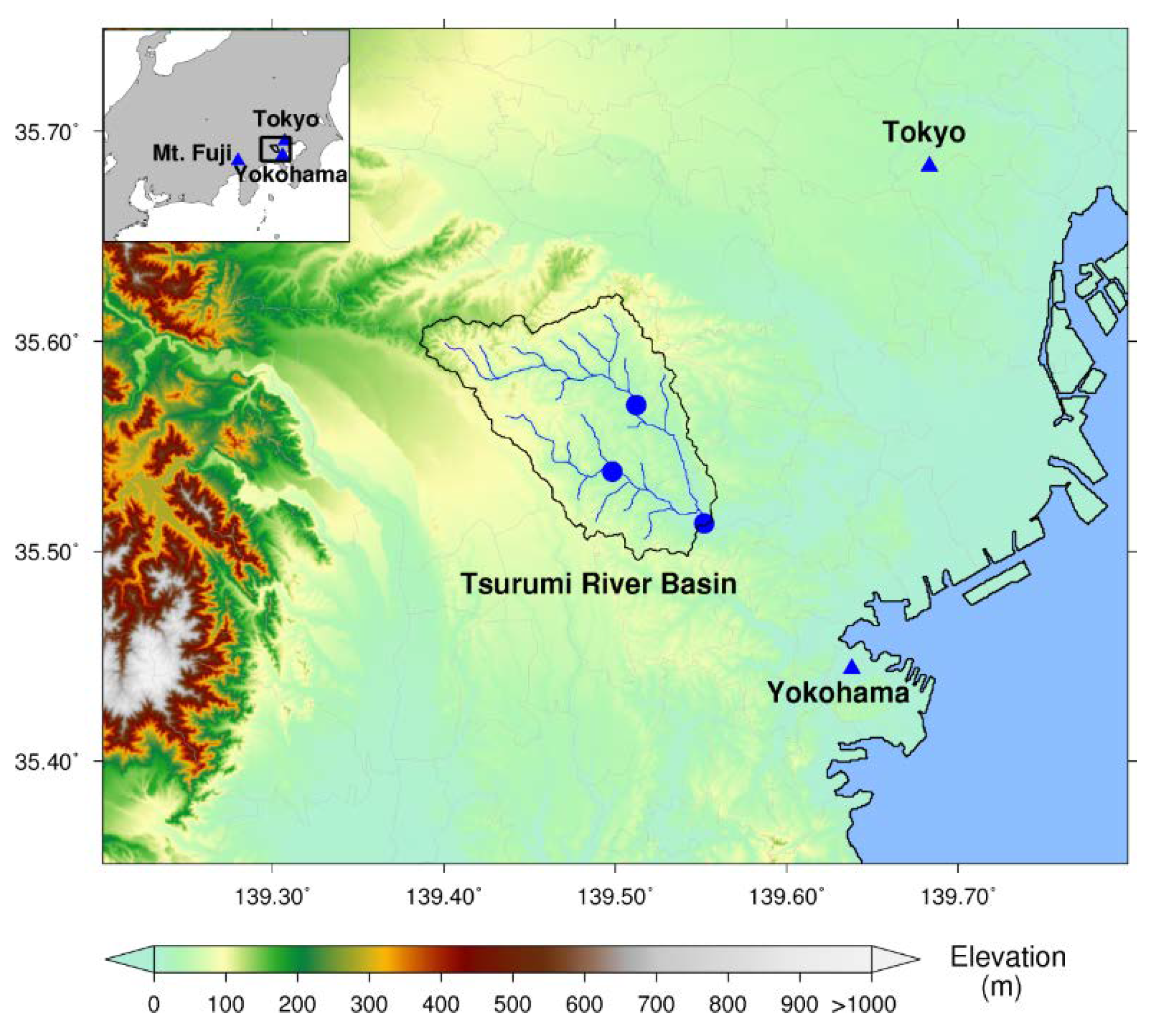
To select the study area, we considered several parameters, e.g., the location of gauging stations in the river basin, river networks, and the availability of radar rainfall data. The Tsurumi River Basin, which is located very close to Yokohama City, Japan (Figure 1), was then selected. Since most of the basin is urban, it can be considered representative of an urbanized river basin. The Tsurumi River is the main tributary in the basin; it originates from a small hill upstream of the basin and finally merges into the sea. There are three gauging stations within the basin: one at the basin outlet, and the others situated along tributaries in the basin. Discharge data for some years can be collected from these stations. The total area of the Tsurumi Basin at its outlet is about 118 km2.
The use of radar rainfall data in the hydrological model at different scales is the key issue in this study. XRAIN data, with spatial and temporal resolutions of 0.25 km and 1 min, respectively, were utilized for most urban areas of the country. Various researchers have reported that the accuracy and reliability of the XRAIN data are consistent with the ground truth data, especially over flat areas [34,35], but that the rainfall estimated over some complex mountain regions may be less accurate because of partial beam blockage [36]. In this study, we did not check or compare the quality of the radar rainfall data, because the accuracy of radar rainfall estimates from XRAIN is generally considered good, and the use of these data for hydrological simulations has already begun [21,22].
Rainfall events were selected based on the following criteria. First, discharge data from the gauging station at the outlet of the Tsurumi River Basin were checked during the summer for 4 years. After checking the discharge pattern of those years, we found that the peak of the hydrograph crossed 100 m3/s several times during the selected years at the outlet of the basin, which is likely indicative of a higher intensity of rainfall. Therefore, several rain events were selected if the peak discharge of one hydrograph at the outlet of basin was more than 100 m3/s; the maximum peak discharge at the outlet was found to be 700 m3/s. Overall, 20 rainfall event cases for different time periods were selected from 2012 to 2015 for the Tsurumi River Basin (Table 1). The total time period of each event was fixed based on the shape of the hydrograph of the gauging stations and corresponding rain event. The total time duration of each event was more than 9 h, with a maximum duration of 45 h.
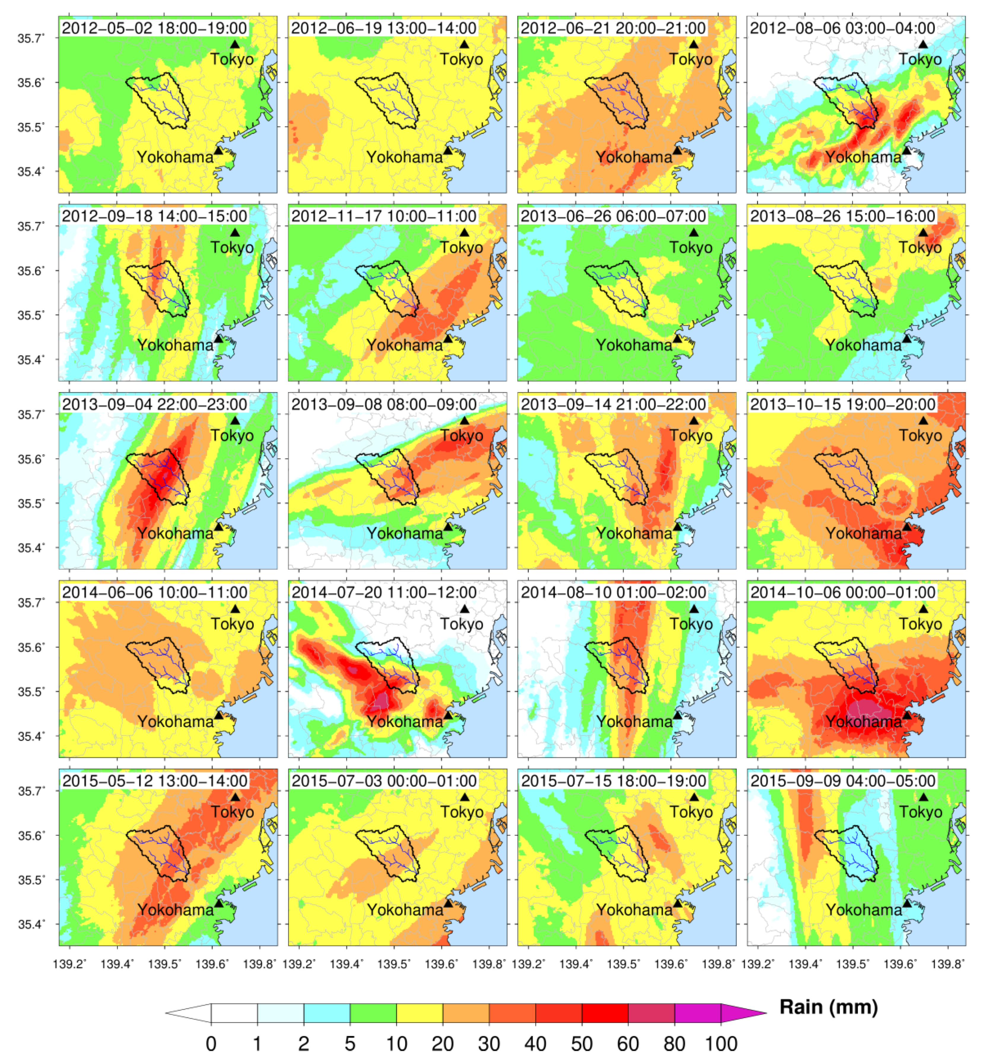
Rainfall distributions and their patterns were analyzed for each case, and they were found to be different. Figure 2 shows the 2-h cumulative rainfall during the peak rainfall over the basin. It can clearly be seen that the rainfall distribution type and pattern are very different for each event. In some cases, rainfall distributions were convective or isolated, while in others, rainfall systems were widespread, mostly as a result of cyclonic activities. Therefore, we broadly categorized rain event cases into two classes (Table 1) according to their patterns and types: convective (localized or isolated) (CR_N) and widespread (WR_N). The localized type of rainfall pattern includes convective and isolated storms as well as concentrations of rainfall echoes in a small area, while widespread rainfall patterns were uniformly distributed and covered large areas. The utilization of these categories in runoff simulations is significant, as it can help answer our earlier questions about whether the same spatial scale needs to be utilized in the simulation and whether a single, optimal spatial scale for rainfall data can be used to model different types of rainfall events.
2.2. Hydrological Model
There are several hydrological models available worldwide with specific targets and goals; each has advantages and disadvantages for hydrological applications. While all hydrological models can be used for simulation, we considered some important points while choosing the model in this study. For example, the selected model should be conducive to the use of radar rainfall data with very high temporal and spatial resolutions (i.e., 5-min and 250-m). The computation time should be as low as possible. The simulated discharge should possess a high temporal resolution, and the model should be available freely for research purpose. To fulfill the objective of the study, we adopted HEC-HMS, which is a model that is freely available for research purposes. It is a simplified model that can be used in a lumped and quasi-distributed manner to simulate high-resolution hydrological responses of a watershed subject with given high-resolution hydrometeorological inputs. These features render the HEC-HMS conducive to the achievement of our study goals. The model was developed by the U.S. Army–Hydrologic Engineering Center; it is designed to simulate the complete hydrological processes of a dendritic watershed system [37] and can be used for both continuous and event-based modeling for a wide variety of watersheds [38].
There are four major components in the model: the basin model, meteorological model, control specifications, and time series input data [39]. The basin model describes the different elements of the hydrological system, such as the sub-basin, reach, junction, reservoir, diversion, source, and sink, and each of these elements needs some parameters to define their interaction in a hydrological system. For the meteorological component, precipitation is a key point for simple event simulations, although there are other meteorological parameters that can be used for continuous simulation. Control specifications are designed to control the time interval of the simulation of any event. The details of the model structures are given in the technical reference manual [37] and the user’s manual [39] of the HEC-HMS, which has been used for a variety of analysis and engineering studies due to its flexibility and applicability in other regions to simulate rainfall-runoff processes [5,17,18,19,20,22,23,40,41,42,43,44,45,46]. The model looks applicable for predicting hydrological responses using radar rainfall during extreme storm events over Japanese river basins [19,20].
2.2.1. Model Set-Up
In the HEC-HMS, there are different processes that must be followed. Topography and watershed information are basic but important data to set-up the model. We used 10-m digital elevation model data downloaded from the website of the Geological Survey Institute. Different methods have been applied to calculate runoff volume, surface runoff, and base flow in the simulations in previous studies [5,17,18,19,20,40,41,42,43,44,45,46]. Each method has its advantages and disadvantages. In this study, we are not interested in comparing all the available methods; therefore, a single method was selected for each process, based on data availability and suitability, during the model set-up. Selected parameters and methods for the modeling of the river basin are shown in the Table 2. We used the gridded U.S. Soil Conservation Service curve number (SCS CN) that was developed to estimate direct runoff. It is a simple, widely used, and efficient method for determining the approximate amount of runoff from a rainfall event. The Modified Clark (ModClark) method was used for transforming excess precipitation into surface runoff. The Muskingum–Cunge standard method was used to simulate flow in open channels, and the exponential recession method was selected for modeling base flow. The mathematical explanations for each method have been described in previous studies [5,17,18,19,20,37,38,40,41,42,43,44,45,46], and the processes followed are described in the HEC-HMS quick guide [39].
Therefore, because we selected various methods for use in each part of the model set-up for the basin, we had to set the initial conditions of the key parameters for each method before conducting the simulations. In the case of the gridded SCS CN, an initial abstraction ratio (AR) and potential retention scale factor (SF) can be defined. The default AR suggested by the SCS is 0.2, but this value can vary down to 0.05 for the runoff calculation [41,43]. This method should only be used with the ModClark unit hydrograph transform method. SF is set to 1 as the default value in the model, and it can vary down to 0.10 [42]. Therefore, the initial values of AR and SF were set to 0.2 and 1.0, respectively.
The transformative method is used to calculate the runoff from excessive precipitation. ModClark is a linear quasi-distributed unit hydrograph method that can be used with gridded meteorological data [23]. The time of concentration (TC) and storage coefficient (SC) are essential parameters, and their ranges vary depending on the different factors of the given watersheds. The initial parameters of these values were calculated using the SCS method [11]. These parameters were very sensible for the peak discharge, and the minimum and maximum range was 0.01 to 1000 h in the flow computations with this model [37].
Muskingum–Cunge standard method was used in routing modeling. Cross section shape was selected as trapezoid type and side slope fixed 1.0 for all sub-basins. Manning’s coefficient is an important parameter that can be the average value for the whole reach. It can be estimated from pictures of streams with known roughness coefficients. It should be noted that Tsurumi River is located very close to Yokohama City and most of the basin can be considered representative of an urbanized river basin. Hence, it was set to 0.025 for all sub-basins and all events because it is a natural channel with significant amounts of coarse sediment and minimal meandering.
In baseflow modeling, the recession method is generally more applicable to shorter duration periods for watersheds where the volume and timing of the base flow are strongly influenced by the precipitation event itself. In this method, the initial discharge (ID), ratio to peak (RP), and recession constant (RC) are the key parameters that can be selected based on the discharge data information at outlet of the basin. ID is the flow at the start of the storm; RC is basically describing the rate of baseflow decay; and RP is the rate at which the baseflow recedes between storm events. RP and RC can vary based on the condition of the land use and soil type [45]. We collected discharge data at the outlet of each sub-basin for each selected event and selected the average of the ID before starting the rain modeling. RP and RC were calculated using the recession constant method [37] and also used in the model.
Many meteorological variables have been considered in large-scale hydrological models and are applicable for long-term averages (e.g., mean monthly or annual discharges), although exceptions exist [47,48,49]. Hence, meteorological variables can play an important role during the long-term continuous simulation of a watershed. In this study, we considered 20 independent events for the hydrological simulation, and the total simulation hours of these events vary from 20 to 54 h. Moreover, we focus on the peak discharge simulation (surface flow) of these separate events. For the meteorological input data to set-up the model, only radar rainfall data were used; other meteorological data were excluded in this study. Events from different periods were considered; hence, we believe that excluding other meteorological parameters in the model should not result in a remarkable error for the selected events.
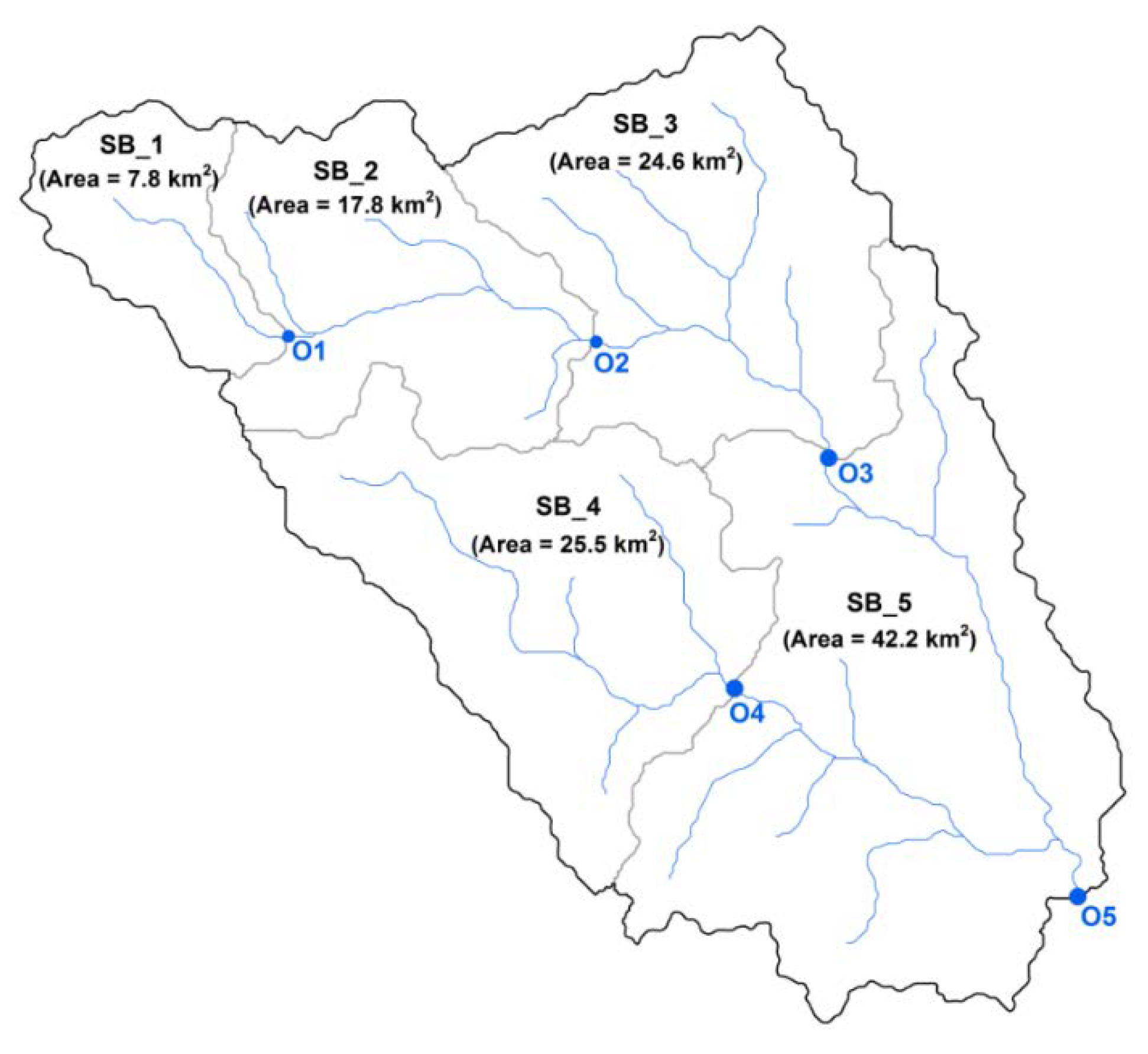
Three gauging stations are located inside the Tsurumi River Basin and are considered for the validation and calibration of the simulated hydrological results. One advantage of the HEC-HMS model is that it can be applied at the sub-basin level. Therefore, considering the features of the model, gauging stations, and topography, five sub-basins were generated within the Tsurumi River Basin. Each sub-basin has different areas, and some have gauging stations at their outlets. The delineated sub-basins, their outlets, and their approximate areas are shown in Figure 3.
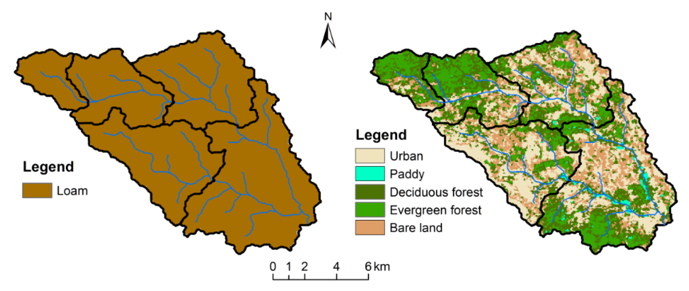
In this study, soil-type data were downloaded from the Harmonized World Soil Database (HWSD). According to this data, the entire basin is comprised of loam-type soil (Figure 4). The HWSD has been used in HEC-HMS in previous studies [19,20]. There are various types of soil classifications, each with its own infiltration capacity. In the hydrological model, these were categorized into hydrological soil groups ranging from “A” to “D”. The Tsurumi River Basin represents the “A” type based on its soil characteristics. Land-use data were taken from the Japan Aerospace Exploration Agency’s Earth Observation Research Center ALOS/ALOS-2 project. High-resolution land-use data show that the basin is mainly dominated by urban areas, but includes forests, bare land, and small areas of paddy fields (Figure 4). These land-use and soil-type datasets are generated from different sources and have been used in the HEC-HMS model in many studies [5,17,18,19,20,40,41,42,43,44,45,46]. The two datasets were considered in the creation of the SCS CN at each grid of the selected basin. The land-use profile of the basins indicated that the majority of their land was urban, with coverage of bare land and forests.
2.2.2. Optimization of Model Parameters
The optimizations of parameters have been done in different ways in several studies. In some studies, optimizations of the parameters are fixed for each event case [41,42,43], while in other studies they are fixed for all events [19,44,45,46]. Of course, parameters can be optimized for single events first, and they can then be applied to other selected events. It should be noted that all the selected events represent different time periods, and each one represents a special case. It is difficult to obtain detailed information on the boundary conditions of these selected events. For example, the soil moisture conditions just before the extreme events may play an important role in contributing to the runoff and initial flow at the river. Therefore, we tried to optimize the parameters for each event separately so that the simulation result could better approximate the real data for each case. Separate optimization of certain parameters in each event may show the deviating range of a parameter in a given basin, the average of which can be used for continuous simulation of other watersheds if similar conditions appear.
The observed hourly discharge data from the three gauging stations inside the basin were extracted and used to develop a good correlation between the observed and simulated discharge. The model parameters AR and SF of the gridded SCS CN, TC, and SC in ModClark, and RC and RP of the recession method, were optimized. The same initial parameters were used in each experiment, and the optimization range of the latter was shown in Section 2.2. Many studies have shown that the range of the model parameters varies greatly [25,37,41,42,43,45,46], and matching the simulated discharge and the observed peak discharge was the key point of this one. Therefore, with the given maximum and minimum range of each model parameter, all selected parameters were optimized using the Univariate Gradient optimization package and peak-weighted root mean square error method during the model set-up. This style of optimization has been used in many studies [5,46] due to its simplicity. However, there are many more methods by which to optimize model parameters; these are not discussed further in this study.
2.3. Assessment Tools
Assessment tools are very important for understanding the difference between simulated and observed data and are often selected based on objectives and goals. The selection of events is basically related to extreme values. Therefore, it is important to check the performance of high peaks in the data. The Nash–Sutcliffe efficiency (NSE), percent absolute error (PAE), percent relative root mean square error (PRRMSE), and percent bias (PBIAS) are key assessment tools used in the analysis [5]. The mathematical descriptions of these tools are shown in Equations (1)–(4):
Nash–Sutcliffe Efficiency (NSE)
Percent Absolute Error (PAE)
Percent Relative Root Mean Square Error (PRRMSE)
Percent Bias (PBIAS)
where and are the observed and estimated discharge rate, respectively, and is the mean of the given data points (N). If the multiplication by 100 in all of the equations is ignored, the range of the NSE varies from −∞ to 1, with NSE = 1 being the optimal value for the comparison test (indicating perfect model performance). Similarly, the ranges of the PAE and PRRMSE vary from 0 to +∞, with 0 being the optimal value, and the range of PBIAS varies from 0 to ±∞, with 0 being the optimal value. These values are converted into percentages herein.
3. Results
3.1. Evaluation of the Model Performance
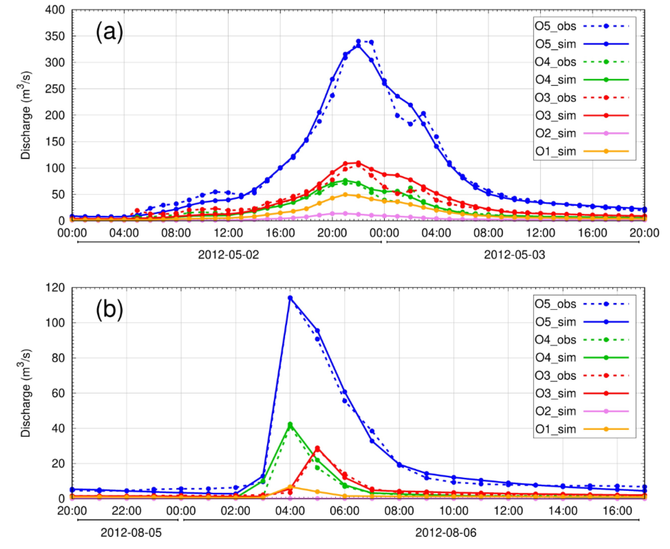
Once the model was built for the Tsurumi River Basin, simulations were performed and compared to the real data for each event. Figure 5 shows the observed and simulated time series discharge data for the widespread rain (WR) event of 2–3 May 2012, and the convective rain (CR) event of 5–6 August 2012, at the sub-basin outlet of the river basin. Two more sub-basins (O1 and O2) were defined in sub-basin O3 to verify the simulated results in different areas of the sub-basin. There was no discharge record at the sub-basin outlets of O1 and O2. All five sub-basins have different areas (Figure 3); sub-basins O3, O4, and O5 have gauging stations at their outlet points (Figure 1). Comparisons of the observed (Obs) and simulated (Sim) time series data clearly show the very good harmony between the two for both events. NSE, PAE, PRRMSE, and PBIAS were calculated at the three outlets of the sub-basins. Statistical tools for the WR_N1 case of 2–3 May 2012, and the CR_N1 case of 5–6 August 2012 at the outlet of basin O5 are 98%, 9.2%, 16%, and 1.1% and 99%, 10.5%, 3.1%, and −0.4%, respectively; for the sub-basin outlets O3 and O4, those for WR_N1 are 78%, 20.6%, 10.8%, and –4.7% and 92%, 15.9%, 6.7%, and 1.1%, respectively; for CR_N1, they are 97%, 16.4%, 1.0%, and −3.2%, and 94%, 25.0%, 2.24%, and −9.9%, respectively. Overall, NSE is more than 90% at all the outlets of the river basin for these two different events. The maximum peak discharge rate is also double that of the CR case. Hence, PRRMSE appears to be higher in the case of a WR event. PBIAS and PAE look similar in both cases. This statistical comparison clearly shows a good performance of the model for the selected outlet of the basin. Similar analyses were applied for the other remaining events. A good relationship was obtained between the observed and simulated time series discharge data at the outlet of three sub-basins (O3, O4, and O5) for each event. The remaining outlet of the ungauged sub-basin also appears to give reliable discharge data for the selected time period of each event.
All selected events were categorized into WR and CR cases. Therefore, an evaluation test was done for each event separately at the gauged sub-basins of the Tsurumi River Basin. Summaries of the assessment tools for the model evaluation are shown in Table 3 and Table 4 (WR and CR cases, respectively). Overall, the simulated discharge over the Tsurumi River Basin for rain events of different time periods appears to be reliable when compared with the observed discharge data at the three gauging stations. The average NSE was found to be about 90% in both cases. Other statistical parameters seem to be more-or-less similar in both cases. However, the statistical assessment tools are slightly better in the case of WR events. Normally, WR events have a long duration and distribute smooth rainfall across the basin. In contrast, CR cases are short and peak rainfall is not high for a very long duration.
The variation in the ranges of the model parameters is discussed in Section 2. The model parameters were optimized during the simulation to achieve good statistical results. Table 5 shows the average optimized model parameters with their standard deviations for all 20 events for the different sub-basins of the Tsurumi River Basin. The AR and RP values are about 0.12 and 0.10 for all sub-basins, and are almost the same across each sub-basin. However, SF, TC, and SC are highly variable in each sub-basin.
3.2. Spatial Resolution of Radar Rainfall Data
In the hydrological simulation, the default spatial resolution of XRAIN data (250 m) was used as the input, and we used radar rainfall at different spatial resolutions without changing the optimized parameters for each event in the model to allow us to compare the results when using different resolutions. A number of interpolation techniques for reproducing the spatial continuity of rainfall fields have been described in the literature [6,18,50,51,52,53,54,55]. These techniques are normally divided into two approaches: deterministic and geostatistical. The most frequently used deterministic methods are nearest neighbor, inverse distance weighting, Thiessen polygon, and Kriging, which are fairly straightforward interpolation techniques that provide reliable results [18,52,53,54]. Some studies also apply a geostatistical approach to interpolate the spatial and temporal resolution of the rainfall data [7,25]. However, each method shows some biases when compared to real datasets [50,52,53,54,55]. Spatial interpolation techniques basically obtain fine resolution data from the lowest amount of available data [52,53,54,55], and they differ in their assumptions or perspectives (local vs. global).
In this study, we first used very high spatial resolution XRAIN data in the model. It should be noted that XRAIN has 250-m spatial resolution, but we want to make the data coarser to compare it with data from previous research [6,18,50,51,52,53,54,55]. Hence, our purpose is to rescale the radar rainfall data into different spatial resolutions for hydrological applications. In addition, in areas in which dense data are lacking, the aforementioned interpolation techniques could be used. Rescaling the data from fine to coarse resolution using the nearest neighbor approach should be straightforward, although scaling them from coarse to fine resolution would be difficult. It should be noted that the temporal resolution of radar rainfall is constant, so the rescaling process is not expected to significantly change the data herein.
3.2.1. Rescaling of Radar Rainfall Data
Default radar rainfall data were rescaled at six different spatial resolutions (i.e., 0.5, 1.0, 1.5, 2.0, 3.0, 4.0, and 5.0 km). It should be mentioned that the total area of the Tsurumi River Basin is about 118 km2, and the area of the sub-basins varies from about 9 to 45 km2. It is believed that the maximum coarse resolution for a 5-km basin is sufficient. Therefore, we limited the upscaling of the radar rainfall resolution to 5 km in this study.
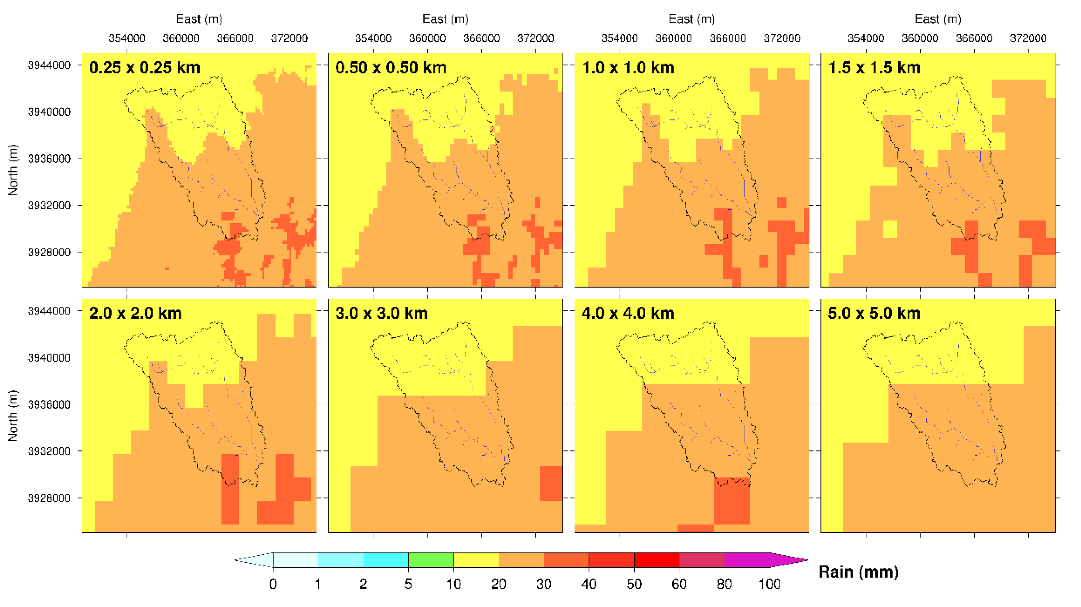
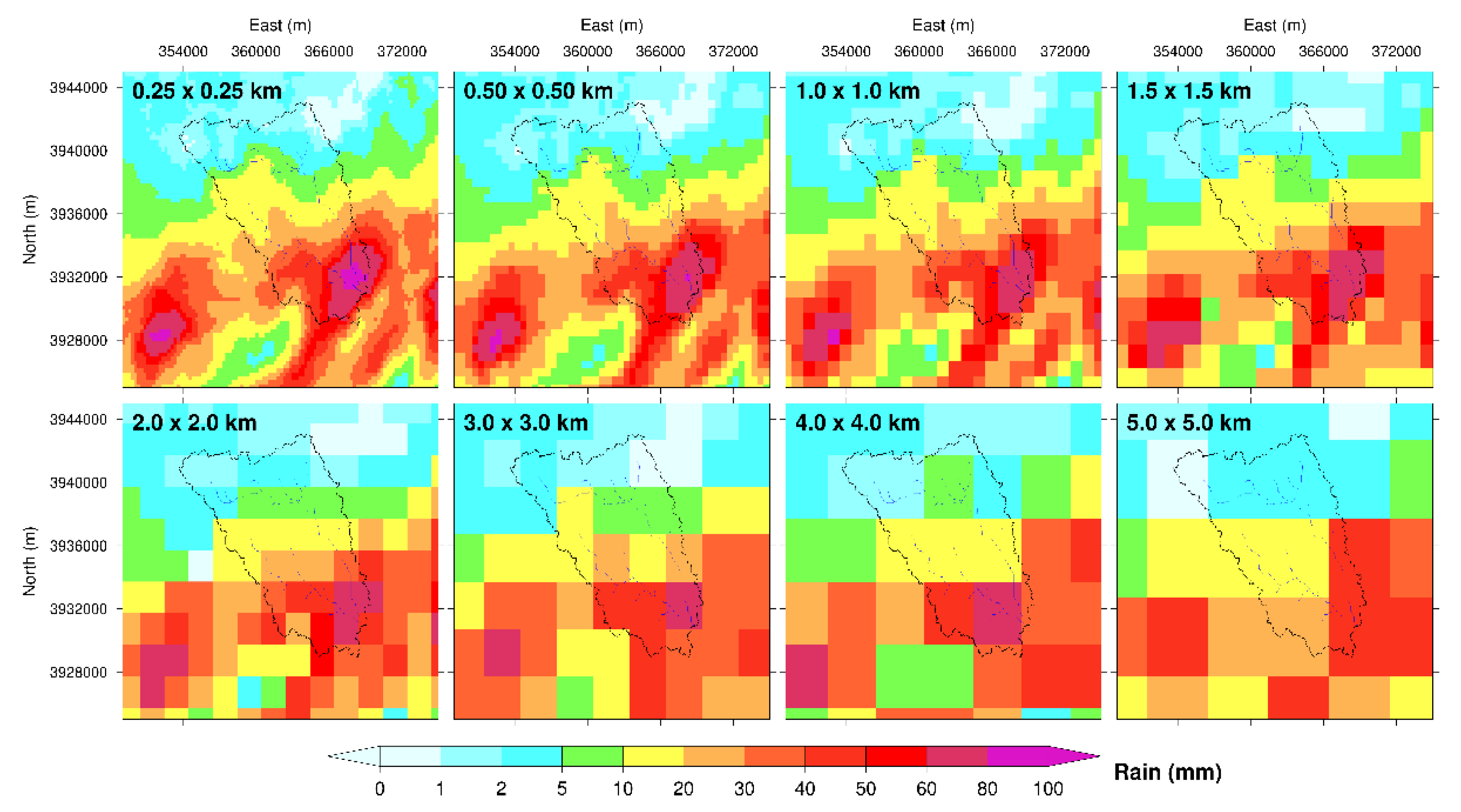
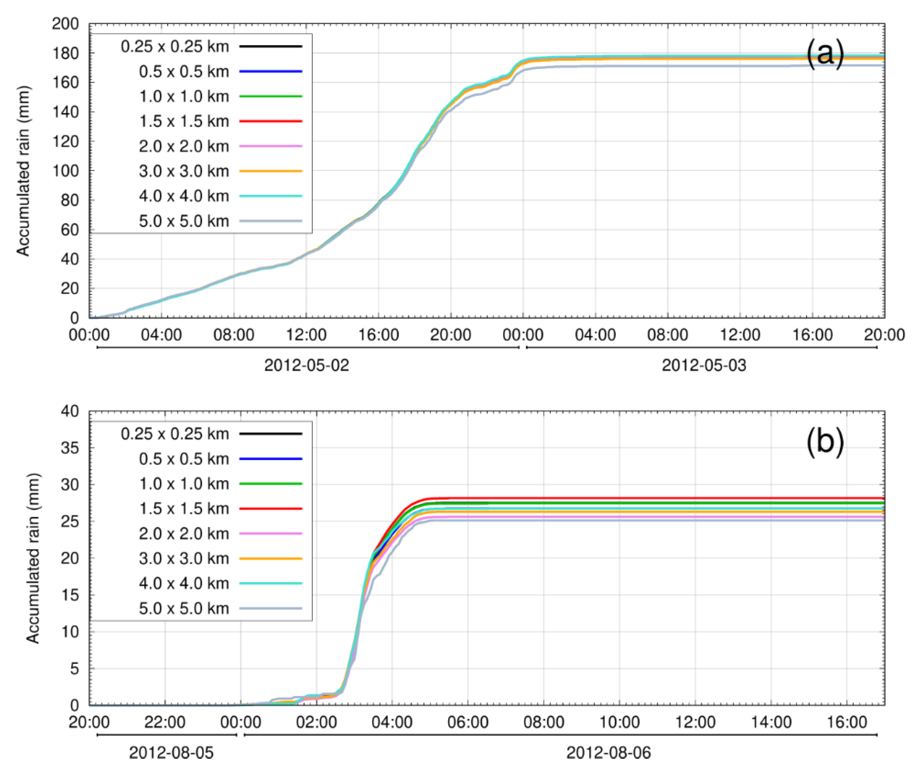
A graphical view of the rescaling at different scales for CR and WR data is shown in Figure 6 and Figure 7. It can be clearly seen that the coarse resolution of the radar rainfall data in the case of a symmetric rainfall distribution has not changed the distribution; however, in the case of a CR event, changes in the rainfall distribution can be seen clearly. To better analyze the effect of different spatial resolutions of rainfall over the basin, the average basin rainfall for each time period of all the selected events was analyzed. Figure 8 shows the time series profile of the basin average accumulated rainfall profile using different spatial resolutions of rainfall. The total accumulated average basin rainfall from the default spatial resolution is about 177.5 mm for the entire 40-h WR_N1 event, and the basin-averaged accumulated rainfall values at 0.5, 1.0, 1.5, 2.0, 3.0, 4.0, and 5.0 km spatial resolutions are 176.9, 177.9, 177.8, 176.6, 176.2, 178.3, and 171.6 mm respectively. The coefficient of variation (%) was calculated considering the standard deviation and mean of those variables. Hence, a ±1.24% coefficient of variation was obtained for the WR_N1 event, which is not a large value. Similarly, in the case of the 20-h CR_N1 event, the average accumulated rainfall from the 0.25, 0.5, 1.0, 1.5, 2.0, 3.0, 4.0, and 5.0 km spatial resolutions are 27.5, 26.8, 27.5, 28.2, 25.6, 26.3, 26.7, and 24.0 mm, respectively. The coefficient of variation in this case is ±4.80%, which is slightly higher than that of the WR_N1 event. Overall, the coefficients of variation persist within 10% of the total rainfall in each event case.
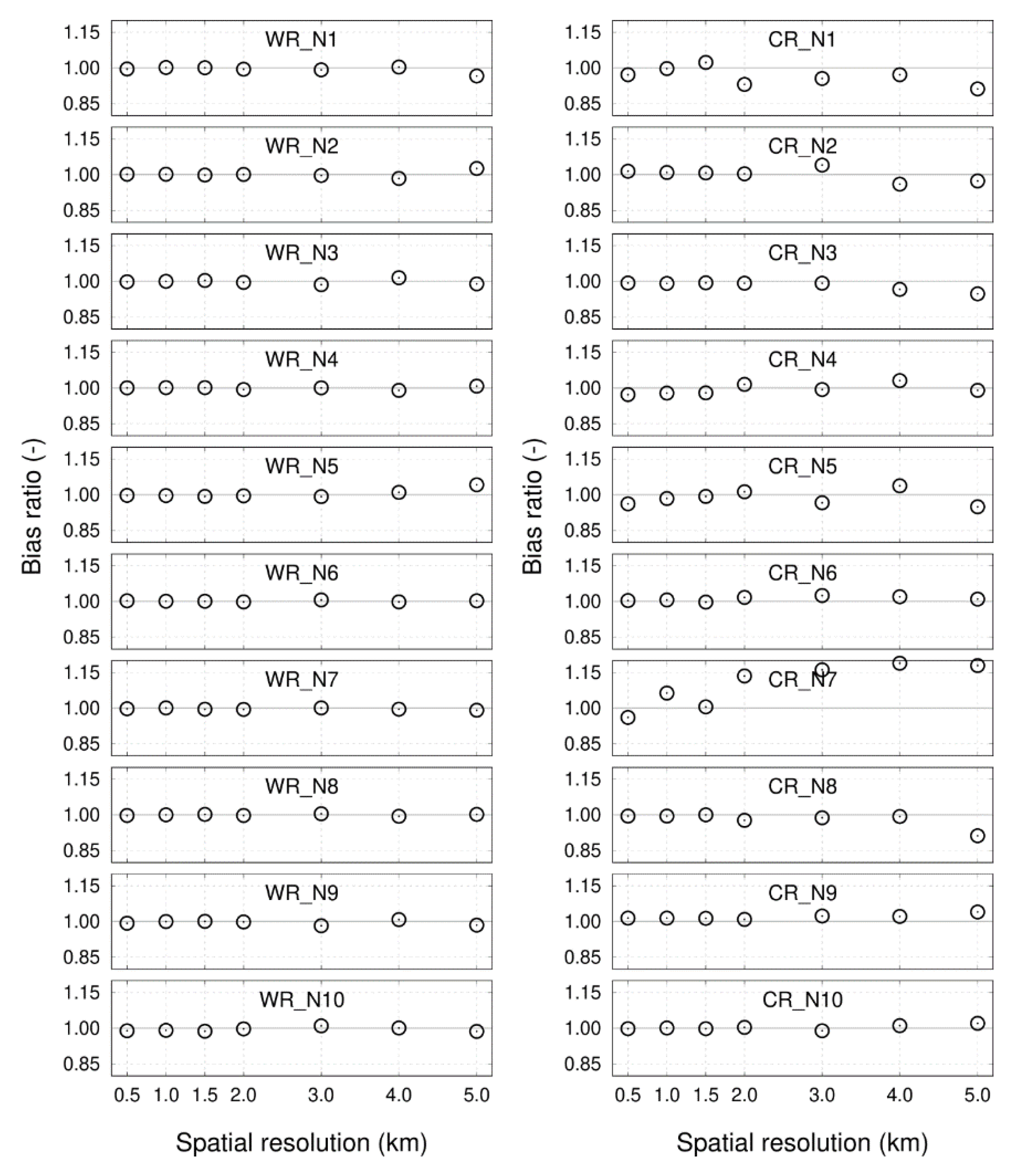
We also calculated the total bias ratio between the default and rescaled basin average radar rainfall data for all the selected rainfall events (Figure 9). The total bias ratio is close to 1 for all the spatial scales of the WR cases. However, a slight fluctuation around 1 can be seen for the CR cases, especially for coarse resolution rainfall data. Hence, based on this statistical analysis of the basin average rainfall data, it can be confirmed that all those rescaled data show similar rainfall patterns within the Tsurumi River Basin. In general, the high resolution of the rainfall data can provide a clearer distribution of rainfall, especially over the rainfall area of the domain. Such detailed information about the rainfall can be missed in coarse resolution data, regardless of which approach is used. We found a fairly close relationship among the rescaled rainfall data using the nearest neighbor approach, which suggests that it may not be necessary to conduct more sophisticated rescaling methods, especially from fine resolution to coarse resolution. However, we did not change the temporal time steps to allow this simple approach to work well with the data.
3.2.2. Inter-Comparison of Simulated Discharge Data
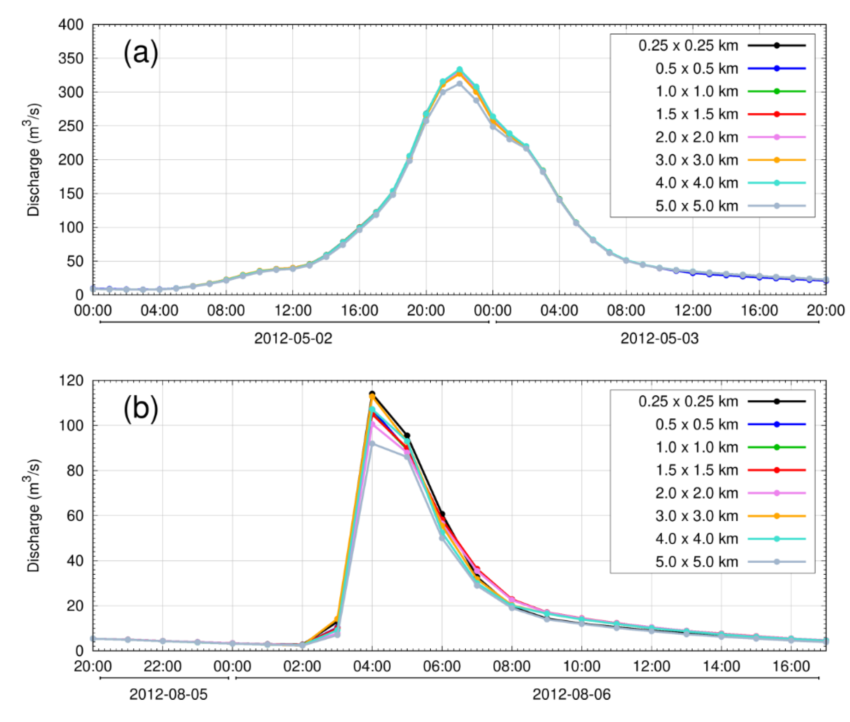
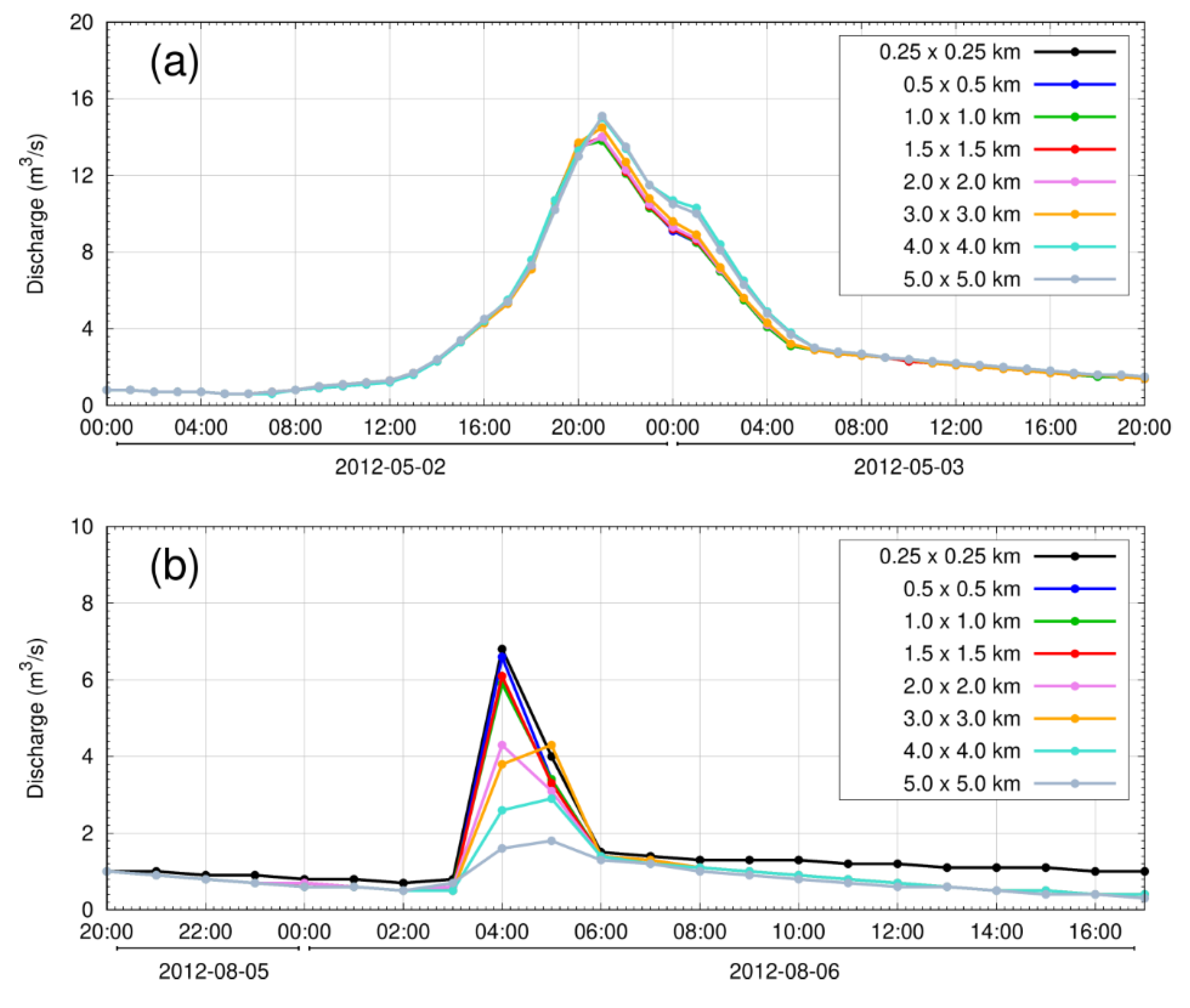
The simulated discharge matched fairly closely with the observed discharge at the outlet of the selected sub-basins based on the default XRAIN data. In this case, those simulated discharges were considered the base references for the analysis of the simulated discharge obtained from different spatial rainfall data inputs. Simulated discharges obtained from different rescaled resolutions of XRAIN data were compared with the reference simulated discharge of all the events. Figure 10 shows an example of the comparison of simulated discharge data obtained from radar rainfall data at different spatial resolutions at the outlet of the basin for WR_N1 and CR_N1 events. It can clearly be seen that there are some differences in each dataset; such differences tend to be higher in the peaks of the hydrographs. Similar plots for sub-basin O2 are shown in Figure 11. There were more deviations on the peak of the simulated hydrograph, especially in the case of CR_N1. The outlet of the entire basin occupies about 118 km2, while sub-basin O2 occupies about 26 km2. It is clear that the time series of the simulated discharge deviates more in the case of the peak hydrograph at the small sub-basin. We also compared the estimated discharge rate of other events for the basin and sub-basin scales to review the effect of the rainfall spatial resolution.
The increased size of the discharge peak is very important, especially for flood risk and management of water resources of the river basin. Therefore, we examined the difference in the peak of the simulated discharge data obtained from the different spatial scales of the rainfall data set in the model. These events were categorized into WR and CR types, and their coefficients of variation are presented in Table 6. These coefficients of variation clearly indicate that some degree of variation can appear when using different spatial resolutions of rainfall data. The fluctuation trend of the coefficient of variation in a small sub-basin (O1, Table 6) is much higher than that in a large sub-basin (O5, Table 6). The small sub-basin sometimes did not receive enough rain to generate runoff, so a proper comparison was not possible (e.g., among CR_N1, CR_N5, and CR_N7 of O1). In general, the average coefficient of variation for the higher discharge peak at each sub-basin shows a different pattern for the WR and CR cases (Table 6). Different spatial resolutions produced different outputs, especially at the peaks of the hydrographs; these output differences were higher for CR cases. To understand the effect of the spatial resolution of rainfall data in hydrological simulations in greater detail, further detailed statistical analyses should be undertaken.
3.2.3. Uncertainties at the Sub-Basin Scale
In the previous section, we evaluated the performance of the peak discharge using different spatial resolutions of XRAIN data over the different sub-basin outlet points of the Tsurumi River Basin. The fluctuation of the discharge rate is higher in small sub-basins than in large sub-basins, and this scenario is seen more often in CR rain events. To better understand the simulated discharge under different spatial resolutions, three statistical tools were applied. The simulated discharge from the default XRAIN data was supposed to be the base reference (equivalent to observed data), and the discharge from the rescaled rainfall data was considered simulated data for the statistical calculation.
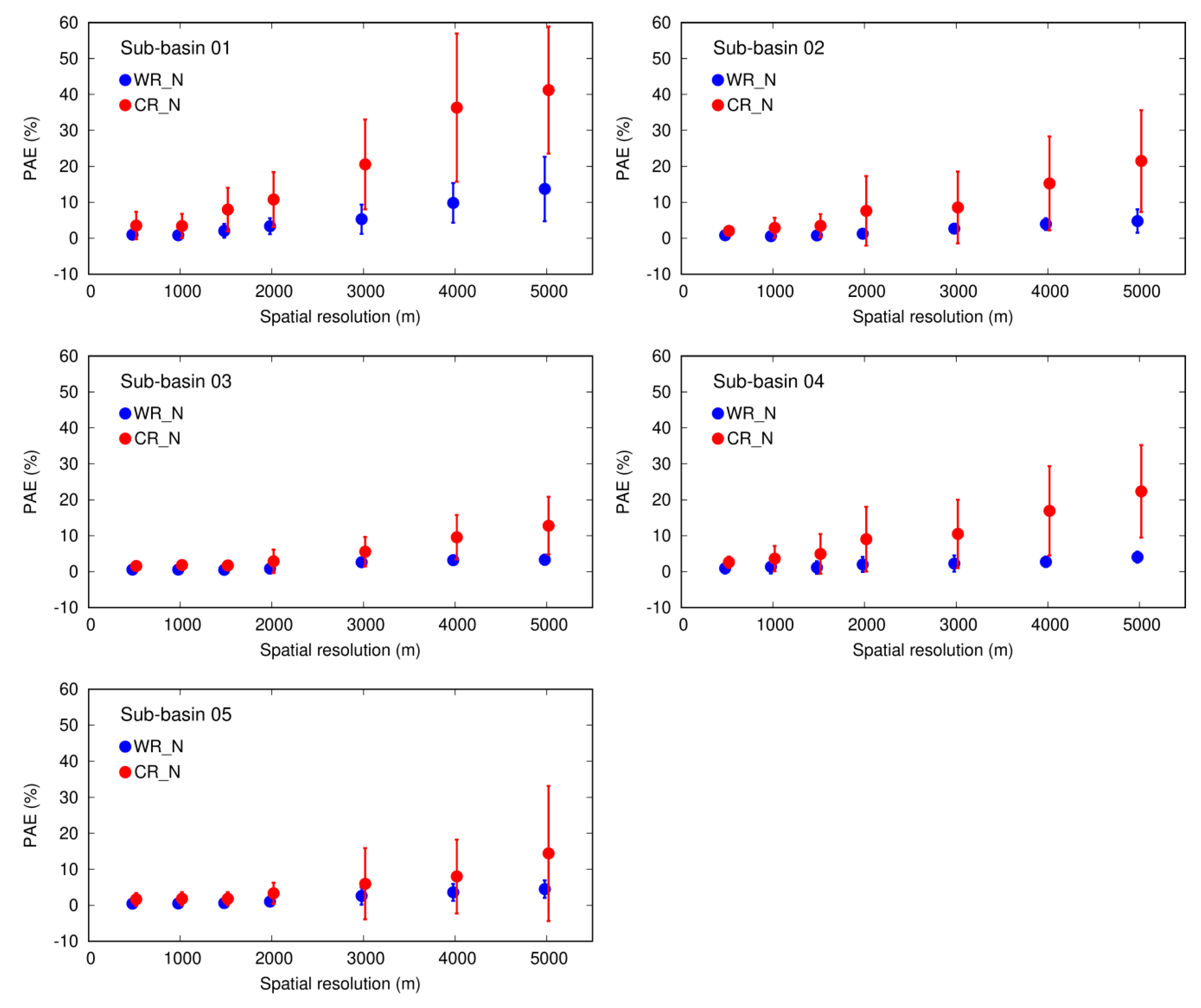
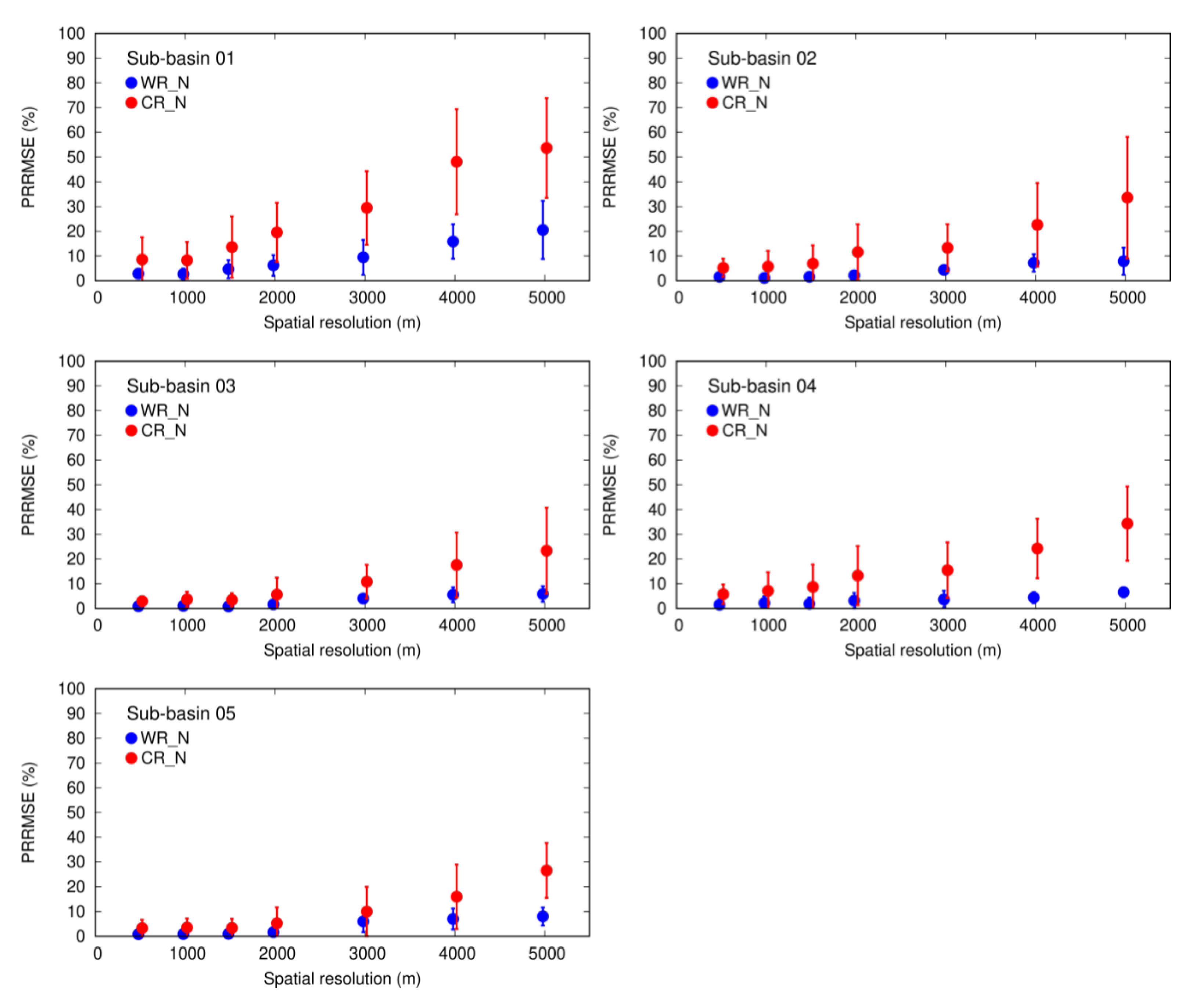
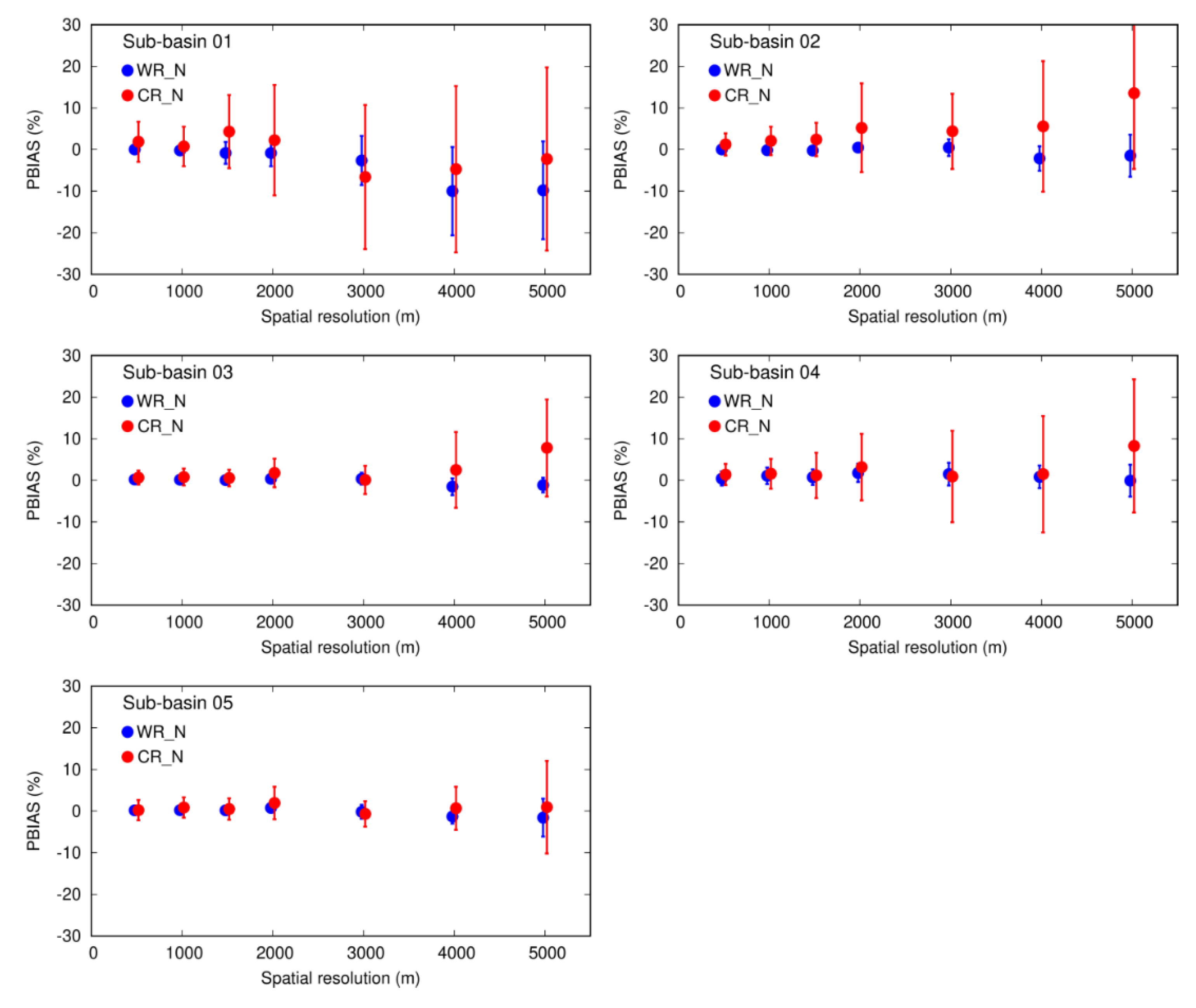
Figure 12, Figure 13 and Figure 14 show the average percentages of the statistical tools—PAE, PRRMSE, and PBIAS—with standard deviations (vertical bars) for the different spatial resolutions of rainfall data for the WR and CR cases. From all these statistical analysis results, it is clear that the effect of the spatial resolution of rainfall data in the hydrological simulation is less sensitive in WR cases than in CR cases for all sub-basins of the Tsurumi River Basin. In general, the fluctuation of the statistical tools appeared at the selected sub-basins in the case of the CR events. However, the degrees of fluctuation of these statistical values are lower for large sub-basins (O4, O5). In contrast, a gentle steady trend of the statistical profile appeared in the case of WR events. If we look at individual sub-basins, more fluctuation of the statistical tools was found for small sub-basins (O1 and O2), especially for the CR cases, which indicates that the changing spatial resolution of CR data is more sensitive for small river basins.
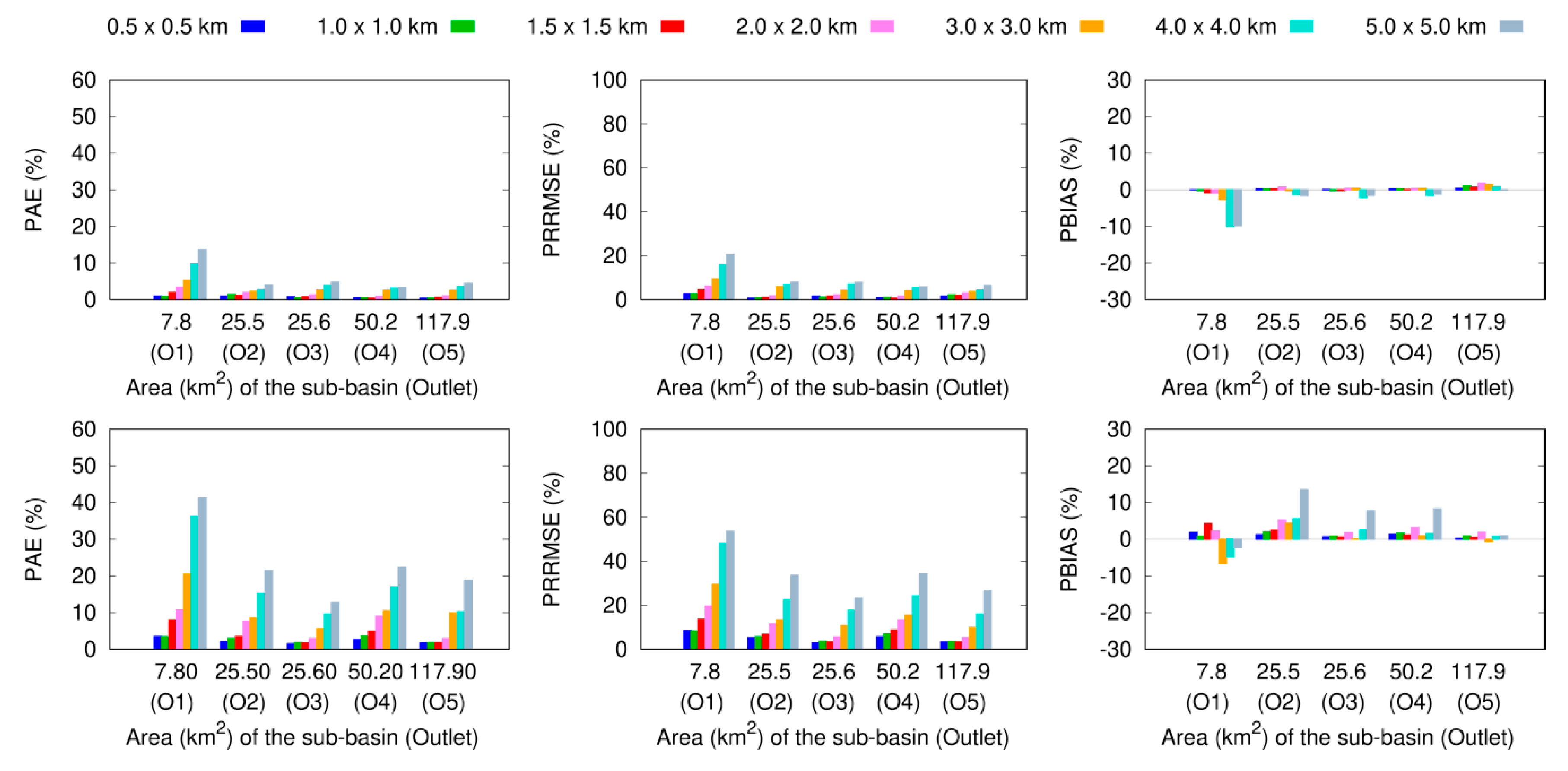
Figure 15 shows the summary of the PAE, PRRMSE, and PBIAS performances for the simulated discharge generated from the rescaled spatial resolution of rainfall over different sub-basins and outlets of the Tsurumi River Basin. Overall, those statistical parameters indicate that the use of rescaled XRAIN data (≤2-km spatial resolution) in hydrological simulations is not very sensitive for all types of rain events at the outlet of the river basin (≈118 km2). In the WR cases, the simulated discharge obtained using ≤5-km rescaled XRAIN data does not indicate a drastic change in the simulated discharge at outlets of sub-basins with areas of more than 25 km2. However, some degree of change in the simulated discharge is possible by using coarser resolution rain data, especially for small sub-basins. We did not find similar trends in the case of convective or isolated rainfall systems. The PAE, PRRMSE, and PBIAS were higher for all sub-basins in the CR cases than in the WR cases, especially for coarser spatial rainfall input (Figure 12, Figure 13 and Figure 14). The simulated discharge varied significantly as the CR resolution changed, and the uncertainty was found to be greater at resolutions above 1 km in most sub-basins smaller than 50 km2. In the case of a very small sub-basin (O1), uncertainty about the simulated discharge was expected to increase when using 2-km rescaled XRAIN data for the WR case, but it appears very sensible for the estimated discharge even when using 0.5-km rescaled XRAIN data for the CR cases.
4. Discussion and Conclusions
Quantitative precipitation estimations from radar observations have improved recently, and composite maps of radar rainfall based on several observation points have been generated at very high spatial resolutions over a specified region with an accuracy that is quite close to ground data [33,34,35]. This represents an improvement in the quality of available radar estimated rainfall data, which is being used in an increasing number of hydrological applications. To study the optimal spatial resolution of radar rainfall data for use in hydrological simulations, we selected the Tsurumi River Basin, which is one of the most important urbanized river basins in Japan; it is located in the heart of Tokyo. Altogether, 20 independent rain events were selected based on higher river discharge at the outlet of the basin. Among those selected rain events, 10 rain events represented isolated rainfall or CR types of patterns, while the remaining events represented the widespread type of rainfall within the Tsurumi River Basin. Of course, the selection of appropriate hydrological models is a key issue in the hydrological community that needs deeper investigation. In this study, we first adopted the HEC-HMS to utilize the very high spatial resolution of XRAIN data as the main input. Simulated results of each event were validated and calibrated separately. To obtain a good correlation between the observed and simulated discharge at the outlet of the sub-basins, some of the model parameters were optimized within the reliable range.
We used the gridded SCS CN, ModClark, and exponential recession as the loss, transform, and base flow methods, respectively, during the model set up. We selected the entire model for HEC-HMS given the suitability of the gridded rainfall data. Previous research showed that the SCS CN and ModClark methods are especially good for radar rainfall data [25], and although there are several other models available in the HEC-HMS, we did not check them because this would have been beyond the scope of this study. However, there have been only a very limited number of studies carried out in Japanese river basins using HEC-HMS; therefore, this study used global reference parameters, particularly for the SCS CN method. The model parameters of each method were optimized to achieve close relationships between these and the observed data. Some of the model parameters were found to be sensitive for this river basin. The most sensitive model parameters were found to be the SF of the loss-gridded SCS CN and the TC and ST of the ModClark method. Previous studies have shown that SF can vary greatly during event analysis [25]. Therefore, variations in SF are common and this parameter should be calibrated before it is applied in any river basin. TC and ST were optimized similarly and were very sensitive in the peak discharge cases [25,40]. The model parameters of the base flow were found to be less sensitive. One important point is that we selected individual events from different periods and based the time and optimization of model parameters on the peak-weighted root mean square error method for each event. This could be one of the reasons why the baseflow parameters were less sensitive than the others.
Several previous researchers studied the use of the spatial resolution of rainfall data in hydrological modeling in two main ways: with rain gauge networks [1,2,6,7,18,29,40,46] and via remote sensing data—e.g., satellite or radar rainfall data [10,14,17,19,20,30,31,32,42]. Some studies used both approaches [3,4,5,12,21,22,23,26]. However, uncertainty can arise during the interpolation of rainfall data from low availability rain gauge networks [1,5,6,7,11]. Additionally, satellite-based rainfall data may have high uncertainties, especially in small to medium river basins [12,13,14]. High spatial resolution rainfall data can be obtained from radar observations; however, previous studies focused on the qualities of radar rainfall data rather than comparing them with simulated hydrological results. We believe that XRAIN has maintained its quality because it has been used for operational purposes [33] and shown that is quite close to ground data [33,34,35]. In this study, detailed research was conducted on the effects of spatial resolutions of radar rainfall on hydrological modeling. We focused our research mainly on simulated hydrological outputs rather than on comparative analyses of rainfall. Moreover, we included several events and separated them by type for the simulations, which had not been done effectively in previous research. Statistical assessment tools showed that the simulated results were better for the WR event cases. This may be due to the wide and smooth coverage of the rainfall distribution. In this study, the temporal resolution of XRAIN data were averaged every 5 min, and the default temporal resolution of the XRAIN data is 1-min. Changing the temporal resolution of the rain events could be another good topic for hydrological applications; however, consideration of the fixed temporal resolution of each rain event is one of the limitations of this study.
Next, we studied the effect of the spatial distribution of rainfall on the simulated discharge at the different sub-basins. The default spatial distribution of XRAIN is 250 m, and the simulated discharge using this dataset was considered as the base reference data for inter-comparison analysis. Rescaling of the spatial resolution of the rainfall data from coarse to high resolution could be very difficult, but the opposite approach is very simple. Therefore, rescaling of the spatial resolution was done based on the nearest neighbor approach. The spatial resolution of the rescaled XRAIN data was set as 0.5, 1.0, 1.5, 2.0, 3.0, 4.0, and 5 km; it can be extended to coarser resolutions, but we divided the Tsurumi River Basin into several sub-basins, with their basin areas varying from about 8 to 50 km2. Hence, considering the basin area, we limited the rescaled rainfall data up to 5 km. We compared the accumulated average basin rainfall of each rescaled XRAIN data event separately. The coarse and fine average rainfall values were similar.
Finally, each rescaled rainfall event was separately considered as the main input for the model. The same optimized mode parameters for each event were used for all the data for those events. All the simulated discharges at different sub-basins were compared with reference discharges obtained from the default XRAIN data (i.e., 250-m spatial resolution). In general, the simulated discharge appears less sensitive using rescaled rainfall data with up to 2-km spatial resolutions for all of the event cases at the outlet of the river basin, which is a range similar to that used in previous studies [25,29,33]. More specifically, we can suggest that the hydrological response using a spatial resolution of ≤5 km may somehow have a similar trend during the case of WR for a river whose basin area is greater than 25 km2. This scenario is slightly different than that reported in previous studies because the type of rain was not classified in the latter.
However, the difference among the hydrological outputs is more noticeable for a small sub-basin (<8 km2). In the case of the isolated rainfall or CR cases, the simulated data error started to increase rapidly using greater than 1-km spatial resolution radar rainfall data over almost all the sub-basins, except its outlet. Overall, the degrees of fluctuation in the statistical results were also higher for CR events than for WR events (Figure 12, Figure 13 and Figure 14) for all sub-basins. In the case of small sub-basins (≤8 km2), the optimal spatial resolution of WR data should be ≤2 km to obtain reliable simulated discharge data, but the optimal spatial scale of the radar rainfall data should be less than 1 km for isolated rainfall or CR cases. This was almost in agreement with previous studies [16,25,32]. When we studied the small sub-basins (8–25 km2), we also found that radar rainfall data with a spatial resolution greater than 1-km may provide high uncertainties in certain cases of CR. This is a finding unique to this study.
We also found that WR was less sensitive in hydrological simulations of medium-scale river basins in Japan and are very curious if a similar approach could be defined for such river basins in other regions. However, radar rainfall data is not yet commonly available in very high-resolution formats. In previous research, all types of rain events were generalized before an appropriate spatial resolution was selected for use in the hydrological modeling. This study clearly shows that the optimum scale of the spatial distribution of rainfall should depend upon the type of rainfall distribution, especially in small urban river basins. Hence, the type of rainfall must be distinguished before an optimum scale for radar rainfall data is selected for hydrological modeling in any river basin.
The importance of the spatial resolution of rainfall in hydrological modeling has been well emphasized [15,16,30]. Since the rainfall distribution varies by season and location, it is not easy to generalize an appropriate spatial resolution of rainfall that can be used for hydrological modeling over any given river basin. However, some events have been analyzed in various countries, and some guidelines have been presented for very small river basins [25]. This study provided a statistical summary based on 20 events over the different sub-basins of the Tsurumi River Basin in Japan. These findings may provide an important basis for the selection of appropriate spatial resolutions of rainfall data for hydrological modeling over similar river basins. We expect to carry out similar analyses for different river basins in different environments so that the optimal scale for spatial rainfall data can be determined on a global basis.
Author Contributions
Conceptualization, S.P.C.; Methodology, S.P.C., T.N., and R.M.; Formal analysis, S.P.C., T.N., and R.M.; Investigation, S.P.C., T.N., and R.M.; Writing—original draft preparation, S.P.C.; Writing—review and editing, S.P.C., T.N., and R.M.; Supervision, T.N. and R.M.
Funding
This research was funded by an internal project under the Storm, Flood and Landslide Research Division, National Research Institute for Earth Science and Disaster Resilience (NIED), Tsukuba, Japan.
Acknowledgments
The authors are thankful to the Ministry of Land, Infrastructure, Transport, and Tourism (MLIT) for publishing the important information and related data sets in their webpages. XRAIN data sets used for this study were provided by MLIT, Japan. The DIAS data set was archived and provided under the framework of the Data Integration and Analysis System (DIAS) through the National Key Technology, Marine Earth Observation Exploration System. The authors acknowledge the support of the NIED. The authors are grateful to the editor and reviewers for their useful suggestions for improvements of the manuscript.
Conflicts of Interest
The authors declare no conflict of interest.
References
- Wilson, C.B.; Valdés, J.B.; Rodriguez-Iturbe, I. On the influence of the spatial distribution of rainfall on storm runoff. Water Resour. Res. 1979, 15, 321–328. [Google Scholar] [CrossRef]
- Dong, X.; Dohmen-Janssen, M.; Booij, M.J. Appropriate spatial sampling of rainfall for flow simulation. Hydrol. Sci. J. 2005, 50, 279–298. [Google Scholar] [CrossRef]
- Cole, S.J.; Moore, R.J. Hydrological modelling using raingauge- and radar-based estimators of areal rainfall. J. Hydrol. 2008, 358, 159–181. [Google Scholar] [CrossRef]
- Yoon, S.S.; Lee, B. Effects of Using High-Density Rain Gauge Networks and Weather Radar Data on Urban Hydrological Analyses. Water 2017, 9, 931. [Google Scholar] [CrossRef]
- Gilewski, P.; Nawalany, M. Inter-Comparison of Rain-Gauge, Radar, and Satellite (IMERG GPM) Precipitation Estimates Performance for Rainfall-Runoff Modeling in a Mountainous Catchment in Poland. Water 2018, 10, 1665. [Google Scholar] [CrossRef]
- Ly, S.; Charles, C.; Degre, A. Different methods for spatial interpolation of rainfall data for operational hydrology and hydrological modeling at watershed scale: A review. Biotechnol. Agron. Soc. Environ. 2013, 17, 392–406. [Google Scholar]
- Muthusamy, M.; Schellart, A.; Tait, S.; Heuvelink, G.B.M. Geostatistical upscaling of rain gauge data to support uncertainty analysis of lumped urban hydrological models. Hydrol. Earth Syst. Sci. 2017, 21, 1077–1091. [Google Scholar] [CrossRef] [Green Version]
- Thorndahl, S.; Einfalt, T.; Willems, P.; Nielsen, J.E.; Veldhuis, M.C.T.; Arnbjerg-Nielsen, K.; Rasmussen, M.R.; Molnar, P. Weather radar rainfall data in urban hydrology. Hydrol. Earth Syst. Sci. 2017, 21, 1359–1380. [Google Scholar] [CrossRef] [Green Version]
- Arsenault, R.; Brissette, F. Determining the Optimal Spatial Distribution of Weather Station Networks for Hydrological Modeling Purposes Using RCM Datasets: An Experimental Approach. J. Hydrometeorol. 2014, 15, 517–526. [Google Scholar] [CrossRef]
- Allegretti, M.; Bertoldo, S.; Prato, A.; Lucianaz, C.; Rorato, O.; Notarpietro, R.; Gabella, M. X-Band Mini Radar for Observing and Monitoring Rainfall Events. Atmos. Clim. Sci. 2012, 2, 290–297. [Google Scholar] [CrossRef]
- Chow, V.T.; Maidment, D.R.; Mays, L.W. Applied Hydrology; McGraw-Hill Book Company: New York, NY, USA, 1988; p. 572. [Google Scholar]
- Xie, P.; Arkin, P.A. An Intercomparison of Gauge Observations and Satellite Estimates of Monthly Precipitation. J. Appl. Meteorol. 1995, 34, 1143–1160. [Google Scholar] [CrossRef] [Green Version]
- Kubota, T.; Ushio, T.; Shige, S.; Kida, S.; Kachi, M.; Okamoto, K. Verification of High-Resolution Satellite-Based Rainfall Estimates around Japan Using a Gauge-Calibrated Ground-Radar Dataset. J. Meteorol. Soc. Jpn. 2009, 87, 203–222. [Google Scholar] [CrossRef]
- Shrestha, N.K.; Qamer, F.M.; Pedreros, D.; Murthy, M.; Wahid, S.M.; Shrestha, M. Evaluating the accuracy of Climate Hazard Group (CHG) satellite rainfall estimates for precipitation based drought monitoring in Koshi basin, Nepal. J. Hydrol. Reg. Stud. 2017, 13, 138–151. [Google Scholar] [CrossRef]
- Berne, A.; Delrieu, G.; Creutin, J.D.; Obled, C. Temporal and spatial resolution of rainfall measurements required for urban hydrology. J. Hydrol. 2004, 299, 166–179. [Google Scholar]
- Einfalt, T.; Arnbjerg-Nielsen, K.; Golz, C.; Jensen, N.-E.; Quirmbachd, M.; Vaes, G.; Vieux, B. Towards a roadmap for use of radar rainfall data in urban drainage. J. Hydrol. 2004, 299, 186–202. [Google Scholar]
- Gao, Y.; Chen, Y.; Zhang, L.; Peng, T. Radar-Rainfall Estimation from S-band Radar and its Impact on the Runoff Simulation of a Heavy Rainfall Event in the Huaihe River Basin. J. Meteorol. Soc. Jpn. 2016, 94, 75–89. [Google Scholar] [CrossRef] [Green Version]
- Chen, T.; Ren, L.; Yuan, F.; Yang, X.; Jiang, S.; Tang, T.; Liu, Y.; Zhao, C.; Zhang, L. Comparison of Spatial Interpolation Schemes for Rainfall Data and Application in Hydrological Modeling. Water 2017, 9, 342. [Google Scholar] [CrossRef]
- P.C., S.; Nakatani, T.; Misumi, R. Hydrological simulation of small river basin in northern Kyushu, Japan during the extreme rainfall event of July 5–6 2017. J. Disaster Res. 2018, 13, 396–409. [Google Scholar] [CrossRef]
- P.C., S.; Nakatani, T.; Misumi, R. Analysis of Flood Inundation in Ungauged Mountainous River Basins: A Case Study of an Extreme Rain Event on 5–6 July 2017 in Northern Kyushu, Japan. J. Disaster Res. 2018, 13, 860–872. [Google Scholar] [CrossRef]
- Chintalapudi, S.; Sharif, H.O.; Xie, H. Sensitivity of Distributed Hydrologic Simulations to Ground and Satellite Based Rainfall Products. Water 2014, 6, 1221–1245. [Google Scholar] [CrossRef] [Green Version]
- Neary, V.S.; Habib, E.; Fleming, M. Hydrologic Modeling with NEXRAD Precipitation in Middle Tennessee. J. Hydrol. Eng. 2004, 9, 339–349. [Google Scholar] [CrossRef]
- Paudel, M.; Nelson, E.J.; Scharffenberg, W. Comparison of Lumped and Quasi-Distributed Clark Runoff Models Using the SCS Curve Number Equation. J. Hydrol. Eng. 2009, 14, 1098–1106. [Google Scholar] [CrossRef]
- Lobligeois, F.; Andréassian, V.; Perrin, C.; Tabary, P.; Loumagne, C. When does higher spatial resolution rainfall information improve streamflow simulation? An evaluation using 3620 flood events. Hydrol. Earth Syst. Sci. 2014, 18, 575–594. [Google Scholar] [CrossRef] [Green Version]
- Ochoa-Rodriguez, S.; Wang, L.P.; Gires, A.; Pina, R.D.; Reinoso-Rondinel, R.; Bruni, G.; Ichiba, A.; Gaitan, S.; Cristiano, E.; Van Assel, J.; et al. Impact of spatial and temporal resolution of rainfall inputs on urban hydrodynamic modelling outputs: A multi-catchment investigation. J. Hydrol. 2015, 531, 389–407. [Google Scholar] [CrossRef]
- Shrestha, N.K.; Goormans, T.; Willems, P. Evaluating the accuracy of C- and X-band weather radars and their application for stream flow simulation. J. Hydroinform. 2013, 15, 1121–1136. [Google Scholar] [CrossRef]
- Goormans, T.; Willems, P. Using Local Weather Radar Data for Sewer System Modeling: Case Study in Flanders, Belgium. J. Hydrol. Eng. 2013, 18, 269–278. [Google Scholar] [CrossRef]
- Gurung, P. Integration of gauge and radar rainfall to enable best simulation of hydrological parameters. Hydrol. Sci. J. 2017, 62, 114–123. [Google Scholar] [CrossRef]
- Schilling, W. Rainfall data for urban hydrology: What do we need? Atmos. Res. 1991, 27, 5–21. [Google Scholar] [CrossRef]
- Berne, A.; Krajewski, W. Radar for hydrology: Unfulfilled promise or unrecognized potential? Adv. Water Resour. 2013, 51, 357–366. [Google Scholar] [CrossRef]
- Price, K.; Purucker, S.T.; Kraemer, S.R. Comparison of radar and gauge precipitation data in watershed models across varying spatial and temporal scales. Hydrol. Process. 2014, 28, 3505–3520. [Google Scholar] [CrossRef]
- Fabry, F.; Bellon, A.; Duncan, M.R.; Austin, G.L. High resolution rainfall measurements by radar for very small basins: The sampling problem reexamined. J. Hydrol. 1994, 161, 415–428. [Google Scholar] [CrossRef]
- Maesaka, T.; Maki, M.; Iwanami, K. Operational Rainfall Estimation by X-band MP Radar Network in MLIT, Japan. In Proceedings of the 35th Conference on Radar Meteorology, Pittsburgh, PA, USA, 26–30 September 2011. [Google Scholar]
- Maki, M.; Iwanami, K.; Misumi, R.; Park, S.G.; Moriwaki, H.; Maruyama, K.I.; Watabe, I.; Lee, D.I.; Jang, M.; Kim, H.K.; et al. Semi-operational rainfall observations with X-band multi-parameter radar. Atmos. Sci. Lett. 2005, 6, 12–18. [Google Scholar] [CrossRef]
- P.C., S.; Misumi, R.; Nakatani, T.; Iwanami, K.; Maki, M.; Maesaka, T.; Hirano, K. Accuracy of quantitative precipitation estimation using operational weather radars: A case study of heavy rainfall on 9–10 September 2015 in the East Kanto region, Japan. J. Disaster Res. 2011, 11, 1003–1016. [Google Scholar] [CrossRef]
- P.C., S.; Maki, M. Application of a modified digital elevation model method to correct radar reflectivity of X-band dual-polarization radars in mountainous regions. Hydrol. Res. Lett. 2014, 8, 77–83. [Google Scholar] [Green Version]
- US Army Corps of Engineers (USACE). Hydrologic Modeling System HEC-HMS: Technical Reference Manual; Hydrologic Engineering Center: Davis, CA, USA, 2000. [Google Scholar]
- US Army Corps of Engineers (USACE). Hydrologic Modeling System HEC-HMS: Application Guide; Hydrologic Engineering Center: Davis, CA, USA, 2015. [Google Scholar]
- US Army Corps of Engineers (USACE). Hydrologic Modeling System HEC-HMS: Quick Start Guide: Version 4.2; Hydrologic Engineering Center: Davis, CA, USA, 2016. [Google Scholar]
- Ghavidelfar, S.; Alvankar, S.R.; Razmkhah, A. Comparison of the Lumped and Quasi-distributed Clark Runoff Models in Simulating Flood Hydrographs on a Semi-arid Watershed. Water Resour. Manag. 2011, 25, 1775–1790. [Google Scholar] [CrossRef]
- Baltas, E.A.; Dervos, N.A.; Mimikou, M.A. Technical Note: Determination of the SCS initial abstraction ratio in an experimental watershed in Greece. Hydrol. Earth Syst. Sci. 2007, 11, 1825–1829. [Google Scholar]
- Montesarchio, V.; Lombardo, F.; Napolitano, F. Rainfall thresholds and flood warning: An operative case study. Nat. Hazards Earth Syst. Sci. 2009, 9, 135–144. [Google Scholar] [CrossRef]
- Woodward, D.E.; Hawkins, R.H.; Jiang, R.; Hjelmfelt, A.T.; Van Mullem, J.A.; Quan, Q.D. Runoff Curve Number Method: Examination of the Initial Abstraction Ratio. In Proceedings of the 2003 World Water & Environmental Resources Congress, Philadelphia, PA, USA, 23–26 June 2003. [Google Scholar]
- Jin, H.; Liang, R.; Wang, Y.; Tumula, P. Flood-Runoff in Semi-Arid and Sub-Humid Regions, a Case Study: A Simulation of Jianghe Watershed in Northern China. Water 2015, 7, 5155–5172. [Google Scholar] [CrossRef] [Green Version]
- Fang, G.; Yuan, Y.; Gao, Y.; Huang, X.; Guo, Y. Assessing the effects of urbanization on flood events with urban agglomeration polders type of flood control pattern using the HEC-HMS model in the Qinhuai River basin, China. Water 2018, 10, 1003. [Google Scholar] [CrossRef]
- Tassew, B.G.; Belete, M.A.; Miegel, K. Application of HEC-HMS model for flow simulation in the Lake Tana basin: The case of Gilgel Abay catchment, upper Blue Nile basin, Ethiopia. Hydrology 2019, 6, 21. [Google Scholar] [CrossRef]
- Kauffeldt, A.; Wetterhall, F.; Pappenberger, F.; Salamon, P.; Thielen, J. Technical review of large-scale hydrological models for implementation in operational flood forecasting schemes on continental level. Environ. Model. Softw. 2016, 75, 68–76. [Google Scholar] [CrossRef]
- Rafee, S.A.A.; Uvo, C.B.; Martins, J.A.; Domingues, L.M.; Rudke, A.P.; Fujita, T.; Freitas, E.D. Large-Scale Hydrological Modelling of the Upper Paraná River Basin. Water 2019, 11, 882. [Google Scholar] [CrossRef]
- López, P.L.; Sutanudjaja, E.H.; Schellekens, J.; Sterk, G.; Bierkens, M.F.P. Calibration of a large-scale hydrological model using satellite-based soil moisture and evapotranspiration products. Hydrol. Earth Syst. Sci. 2017, 21, 3125–3144. [Google Scholar] [CrossRef] [Green Version]
- Szcześniak, M.; Piniewski, M. Improvement of Hydrological Simulations by Applying Daily Precipitation Interpolation Schemes in Meso-Scale Catchments. Water 2015, 7, 747–779. [Google Scholar] [CrossRef]
- Shekhar, S.; Xiong, H. Inverse Distance Weighting; Springer: New York, NY, USA, 2008; p. 600. [Google Scholar]
- Dirks, K.N.; Hay, J.E.; Stow, C.D.; Harris, D. High resolution studies of rainfall on Norfolk Island. Part 2: Interpolation of rainfall data. J. Hydrol. 1989, 208, 187–193. [Google Scholar] [CrossRef]
- Lee, J.; Kim, S.; Jun, H. A Study of the Influence of the Spatial Distribution of Rain Gauge Networks on Areal Average Rainfall Calculation. Water 2018, 10, 1635. [Google Scholar] [CrossRef]
- Cheng, M.; Wang, Y.; Engel, B.; Zhang, W.; Peng, H.; Chen, X.; Xia, H. Performance Assessment of Spatial Interpolation of Precipitation for Hydrological Process Simulation in the Three Gorges Basin. Water 2017, 9, 838. [Google Scholar] [CrossRef]
- Avila, F.B.; Dong, S.; Menang, K.P.; Rajczak, J.; Renom, M.; Donat, M.G.; Alexander, L.V. Systematic investigation of gridding-related scaling effects on annual statistics of daily temperature and precipitation maxima: A case study for south-east Australia. Weather Clim. Extrem. 2015, 9, 6–16. [Google Scholar] [CrossRef] [Green Version]
Figure 1.
Location of the Tsurumi River Basin in Japan. Blue lines and circles denote the river networks and gauging stations throughout the basin, respectively.
Figure 1.
Location of the Tsurumi River Basin in Japan. Blue lines and circles denote the river networks and gauging stations throughout the basin, respectively.

Figure 2.
2-h accumulated rainfall distribution pattern over the Tsurumi River Basin.

Figure 3.
Sub-basin (SB) profile for the HEC-HMS model set-up.

Figure 4.
Soil-type and land-use profile of the Tsurumi River Basin.

Figure 5.
Time series profile of observed (Obs) and simulated (Sim) discharge at sub-basin outlets for the events of (a) 2–3 May 2012 (widespread rain, WR) and (b) 5–6 August 2012 (convective rain, CR).
Figure 5.
Time series profile of observed (Obs) and simulated (Sim) discharge at sub-basin outlets for the events of (a) 2–3 May 2012 (widespread rain, WR) and (b) 5–6 August 2012 (convective rain, CR).

Figure 6.
2-h accumulated rainfall at different spatial resolutions over the Tsurumi River Basin and its periphery at 17:00–18:00 UTC on 5 May 2012.
Figure 6.
2-h accumulated rainfall at different spatial resolutions over the Tsurumi River Basin and its periphery at 17:00–18:00 UTC on 5 May 2012.

Figure 7.
2-h accumulated rainfall at different spatial resolutions over the Tsurumi River Basin and its periphery at 02:00–04:00 UTC on 8 August 2012.
Figure 7.
2-h accumulated rainfall at different spatial resolutions over the Tsurumi River Basin and its periphery at 02:00–04:00 UTC on 8 August 2012.

Figure 8.
Basin-averaged accumulated rainfall profile for the different spatial resolutions for the event of (a) 2–3 May 2012 (widespread rain, WR) and (b) 5–6 August 2012 (convective rain, CR).
Figure 8.
Basin-averaged accumulated rainfall profile for the different spatial resolutions for the event of (a) 2–3 May 2012 (widespread rain, WR) and (b) 5–6 August 2012 (convective rain, CR).

Figure 9.
Total bias ratio of the basin-averaged accumulated rainfall for different spatial resolutions of all 20 rain events (left panel: widespread rain (WR) cases; right panel: convective rain (CR) cases).
Figure 9.
Total bias ratio of the basin-averaged accumulated rainfall for different spatial resolutions of all 20 rain events (left panel: widespread rain (WR) cases; right panel: convective rain (CR) cases).

Figure 10.
Time series profile of the simulated discharge at the outlet of the Tsurumi River Basin for the events of (a) 2–3 May 2012 (WR_N1), and (b) 5–6 August 2012 (CR_N1).
Figure 10.
Time series profile of the simulated discharge at the outlet of the Tsurumi River Basin for the events of (a) 2–3 May 2012 (WR_N1), and (b) 5–6 August 2012 (CR_N1).

Figure 11.
Time series profile of the simulated discharge at the outlet of sub-basin O2 of the Tsurumi River Basin for the events of (a) 2–3 May 2012 (WR_N1), and (b) 5–6 August 2012 (CR_N1).
Figure 11.
Time series profile of the simulated discharge at the outlet of sub-basin O2 of the Tsurumi River Basin for the events of (a) 2–3 May 2012 (WR_N1), and (b) 5–6 August 2012 (CR_N1).

Figure 12.
Percent absolute error profile with the standard deviation (vertical error bar) of the simulated discharge at each sub-basin using different rainfall data spatial resolutions (WR_N: widespread rain (WR) cases; CR_N: convective rain (CR) cases).
Figure 12.
Percent absolute error profile with the standard deviation (vertical error bar) of the simulated discharge at each sub-basin using different rainfall data spatial resolutions (WR_N: widespread rain (WR) cases; CR_N: convective rain (CR) cases).

Figure 13.
Percent relative root mean square error profile with the standard deviation (vertical error bar) of the simulated discharge at each sub-basin using different rainfall data spatial resolutions (WR_N: widespread rain (WR) cases; CR_N: convective rain (CR) cases).
Figure 13.
Percent relative root mean square error profile with the standard deviation (vertical error bar) of the simulated discharge at each sub-basin using different rainfall data spatial resolutions (WR_N: widespread rain (WR) cases; CR_N: convective rain (CR) cases).

Figure 14.
Percent bias profile with the standard deviation (vertical error bar) of the simulated discharge at each sub-basin using different rainfall data spatial resolutions (WR_N: widespread rain (WR) cases; CR_N: convective rain (CR) cases).
Figure 14.
Percent bias profile with the standard deviation (vertical error bar) of the simulated discharge at each sub-basin using different rainfall data spatial resolutions (WR_N: widespread rain (WR) cases; CR_N: convective rain (CR) cases).

Figure 15.
Percent absolute error, percent relative root mean square error, and percent bias profiles of the simulated discharge over the sub-basin and outlet of the Tsurumi River Basin using different spatial resolutions of rainfall data (upper panels: widespread rain (WR) cases; lower panels: convective rain (CR) cases).


Table 1.
Dates, durations, peak discharge, and summary of selected rainfall events.
| SN | Date | Considered Time Period (UTC) | Total Hours | * Peak Q (m3/s) | Summary of Rainfall Event | Name Given | |
|---|---|---|---|---|---|---|---|
| Start Time | End Time | ||||||
| 1 | 2–3 May 2012 | 02:00 02-May | 20:00 03-May | 43 | 340 | Widespread, typhoon-affected, rainfall, long time period | WR_N1 |
| 2 | 19–20 June 2012 | 03:00 19-June | 13:00 20-May | 36 | 273 | Widespread, typhoon-affected, heavy rainfall, long time period | WR_N2 |
| 3 | 21–22 June 2012 | 18:00 21-June | 15:00 22-June | 22 | 239 | Widespread, typhoon-affected, heavy rainfall, short time period | WR_N3 |
| 4 | 05–06 August 2012 | 20:00 05-August | 15:00 06-August | 20 | 114 | Convective, scattered heavy rainfall, short time period | CR_N1 |
| 5 | 18–19 September 2012 | 22:00 18-September | 07:00 19-September | 22 | 107 | Convective, scattered rainfall and widespread rainfall, short time period | CR_N2 |
| 6 | 17–18 November 2012 | 04:00 17-November | 23:00 17-November | 20 | 144 | Convective, scattered rain, long echo type, heavy rainfall, short time period | CR_N3 |
| 7 | 26–26 June 2013 | 00:00 26-June | 23:00 26-June | 24 | 101 | Widespread, moderate rainfall, short time period | WR_N4 |
| 8 | 26–27 August 2013 | 10:00 26-August | 07:00 27-August | 22 | 101 | Widespread, moderate rainfall, short time period | WR_N5 |
| 9 | 04–06 September 2013 | 11:00 04-September | 10:00 05-September | 24 | 332 | Convective, scattered rain, long echo type, heavy rainfall, short time period | CR_N4 |
| 10 | 08–09 September 2013 | 04:00 08-September | 00:00 09-September | 21 | 185 | Convective, scattered rain, long echo type, heavy rainfall, short time period | CR_N5 |
| 11 | 14–15 September 2013 | 15:00 14-September | 16:00 15-September | 26 | 407 | Scattered rain, typhoon affected, heavy rainfall, long time period | CR_N6 |
| 12 | 15–16 October 2013 | 02:00 15-October | 11:00 16-October | 34 | 503 | Widespread, typhoon affected, heavy rainfall, long time period | WR_N6 |
| 13 | 05–07 June 2014 | 21:00 05-June | 23:00 07-June | 51 | 288 | Widespread, moderate rainfall, long time period | WR_N7 |
| 14 | 20–21 July 2014 | 05:00 20-July | 00:00 21-July | 20 | 221 | Convective, scattered heavy rainfall, short time period | CR_N7 |
| 15 | 09–10 August 2014 | 16:00 09-August | 20:00 10-August | 29 | 236 | Convective, scattered rain, long echo type, heavy rainfall, long time period | CR_N8 |
| 16 | 04–06 October 2014 | 19:00 04-October | 02:00 07-October | 56 | 557 | Widespread, typhoon affected, heavy rainfall, long time period | WR_N8 |
| 17 | 12–13 May 2015 | 07:00 12-May | 08:00 13-May | 26 | 265 | Widespread, typhoon affected, heavy rainfall, long time period | WR_N9 |
| 18 | 02–04 July 2015 | 15:00 02-July | 06:00 04-July | 43 | 154 | Widespread, typhoon affected, heavy rainfall, long time period | WR_N10 |
| 19 | 15–17 July 2015 | 13:00 15-July | 10:00 17-July | 46 | 114 | Convective, scattered heavy rainfall, long time period | CR_N9 |
| 20 | 07–09 September 2015 | 15:00 07-September | 20:00 09-September | 54 | 279 | Long echo type, typhoon affected, heavy rainfall, long time period | CR_N10 |
* Peak Q (discharge) represents conditions at the outlet of the Tsurumi River Basin.
Table 2.
Selected components for the HEC-HMS.
| Basin Model | Meteorological Model | Control | Time Series Data | ||
|---|---|---|---|---|---|
| Parameter | Method | Parameter | Method | Time Period | Time Period |
| Loss | SCS CN | Radar rainfall | Gridded data | Selected hours (Table 1) | Discharge data (Table 1) |
| Transform | ModClarck | ||||
| Baseflow | Recession | ||||
| Routing | Muskingum–Cunge | ||||
Table 3.
Average statistical tools at the sub-basin outlets of the Tsurumi River Basin for the case of widespread rain (WR) events.
Table 3.
Average statistical tools at the sub-basin outlets of the Tsurumi River Basin for the case of widespread rain (WR) events.
| Sub-Basin Outlet | NSE (%) | PAE (%) | PRRMSE (%) | PBIAS (%) |
|---|---|---|---|---|
| O3 | 86 (±14) | 23.5 (±9.9) | 40.3 (±17.1) | −5.7 (±12.2) |
| O4 | 88 (±8) | 23.6 (±8.0) | 40.5 (±14.7) | 3.1 (±9.7) |
| O5 | 95 (±5) | 14.9 (±5.9) | 21.9 (±7.5) | 0.6 (±4.8) |
| Average | 90 (±10) | 20.6 (±7.9) | 34.2 (±13.1) | −0.7 (±8.9) |
Table 4.
Average statistical tools at the sub-basin outlets of the Tsurumi River Basin for the case of convective rain (CR) events.
Table 4.
Average statistical tools at the sub-basin outlets of the Tsurumi River Basin for the case of convective rain (CR) events.
| Sub-Basin Outlet | NSE (%) | PAE (%) | PRRMSE (%) | PBIAS (%) |
|---|---|---|---|---|
| O3 | 90 (±5) | 29.2 (±8.8) | 44.1 (±9.7) | −13.9 (±10.4) |
| O4 | 89 (±10) | 28.4 (±12.1) | 50.9 (±30.7) | −2.2 (±7.5) |
| O5 | 91 (±8) | 20.4 (±7.9) | 30.5 (±12.1) | −4.5 (±9.7) |
| Average | 90 (±8) | 26.0 (±9.6) | 41.8 (±17.5) | −6.9 (±9.2) |
Table 5.
Average optimum parameters for the HEC-HMS model for the Tsurumi River Basin.
| Sub-Basin | Loss—Gridded SCS Curve Number | Transform—ModClark | Base Flow—Recession | |||
|---|---|---|---|---|---|---|
| AR (-) | SF (-) | TC (h) | SC (h) | RC (-) | RP (-) | |
| SB_1 | 0.12 (±0.01) | 0.59 (±0.18) | 0.18 (±0.18) | 1.51 (±0.77) | 0.10 (±0.02) | 0.10 (±0.03) |
| SB_2 | 0.12 (±0.01) | 0.60 (±0.19) | 0.40 (±0.41) | 1.39 (±0.82) | 0.10 (±0.02) | 0.10 (±0.03) |
| SB_3 | 0.12 (±0.01) | 0.57 (±0.20) | 0.40 (±0.40) | 1.48 (±0.77) | 0.11 (±0.02) | 0.11 (±0.04) |
| SB_4 | 0.11 (±0.01) | 0.50 (±0.16) | 0.53 (±0.50) | 1.19 (±0.59) | 0.15 (±0.20) | 0.11 (±0.03) |
| SB_5 | 0.12 (±0.03) | 0.65 (±0.17) | 0.78 (±0.61) | 2.52 (±0.96) | 0.18 (±0.25) | 0.10 (±0.03) |
Table 6.
Coefficient of variation of the simulated discharge obtained from different rescaled rainfall data in the model for the outlets of sub-basins in the Tsurumi River Basin.
Table 6.
Coefficient of variation of the simulated discharge obtained from different rescaled rainfall data in the model for the outlets of sub-basins in the Tsurumi River Basin.
| Event | Coefficient of Variation (%) for Sub-Basins | ||||
|---|---|---|---|---|---|
| O1 | O2 | O3 | O4 | O5 | |
| WR_N1 | 1.0 | 1.0 | 0.6 | 1.1 | 1.9 |
| WR_N2 | 3.4 | 0.7 | 0.7 | 1.7 | 1.0 |
| WR_N3 | 3.8 | 2.3 | 4.6 | 2.4 | 2.4 |
| WR_N4 | 4.4 | 3.4 | 1.9 | 1.1 | 0.6 |
| WR_N5 | 9.1 | 3.7 | 1.9 | 1.3 | 2.4 |
| WR_N6 | 3.2 | 1.5 | 1.4 | 1.8 | 1.6 |
| WR_N7 | 2.7 | 0.9 | 0.7 | 2.9 | 2.3 |
| WR_N8 | 2.5 | 0.8 | 1.0 | 0.5 | 1.4 |
| WR_N9 | 12.4 | 3.4 | 3.6 | 1.4 | 3.7 |
| WR_N10 | 1.2 | 2.8 | 2.8 | 3.0 | 2.9 |
| Mean | 4.4 | 2.0 | 1.9 | 1.7 | 2.0 |
| CR_N1 | – | 44.0 | 14.7 | 11.2 | 5.8 |
| CR_N2 | 43.0 | 26.4 | 13.2 | 9.9 | 10.6 |
| CR_N3 | 16.2 | 2.0 | 2.4 | 2.3 | 2.2 |
| CR_N4 | 47.0 | 10.9 | 6.4 | 3.9 | 6.8 |
| CR_N5 | – | 8.7 | 7.9 | 3.5 | 3.6 |
| CR_N6 | 7.4 | 2.5 | 1.3 | 4.4 | 2.0 |
| CR_N7 | – | 48.2 | 9.0 | 44.6 | 3.5 |
| CR_N8 | 23.7 | 12.1 | 3.3 | 9.6 | 3.3 |
| CR_N9 | 37.3 | 4.4 | 2.1 | 2.6 | 1.4 |
| CR_N10 | 18.8 | 5.0 | 4.0 | 3.7 | 3.6 |
| Mean | 27.6 | 16.4 | 6.4 | 9.6 | 4.3 |
© 2019 by the authors. Licensee MDPI, Basel, Switzerland. This article is an open access article distributed under the terms and conditions of the Creative Commons Attribution (CC BY) license (http://creativecommons.org/licenses/by/4.0/).
Share and Cite
MDPI and ACS Style
P. C., S.; Nakatani, T.; Misumi, R. The Role of the Spatial Distribution of Radar Rainfall on Hydrological Modeling for an Urbanized River Basin in Japan. Water 2019, 11, 1703. https://doi.org/10.3390/w11081703
AMA Style
P. C. S, Nakatani T, Misumi R. The Role of the Spatial Distribution of Radar Rainfall on Hydrological Modeling for an Urbanized River Basin in Japan. Water. 2019; 11(8):1703. https://doi.org/10.3390/w11081703
Chicago/Turabian StyleP. C., Shakti, Tsuyoshi Nakatani, and Ryohei Misumi. 2019. "The Role of the Spatial Distribution of Radar Rainfall on Hydrological Modeling for an Urbanized River Basin in Japan" Water 11, no. 8: 1703. https://doi.org/10.3390/w11081703
Note that from the first issue of 2016, this journal uses article numbers instead of page numbers. See further details here.