Characterization and Simulation of a Low-Pressure Rotator Spray Plate Sprinkler Used in Center Pivot Irrigation Systems

Abstract

Spray sprinklers enable to operate at low pressures (<103 kPa) in self-propelled irrigation machines. A number of experiments were performed to characterize the water distribution pattern of an isolated rotator spray plate sprinkler operating at very low pressure under different experimental conditions. The experiments were performed under two pressures (69 kPa and 103 kPa) and in calm and windy conditions. The energy losses due to the impact of the out-going jet with the sprinkler plate were measured using an optical technique. The adequacy to reproduce the measured water distribution pattern under calm conditions of two drop size distribution models was evaluated. A ballistic model was used to simulate the water distribution pattern under wind conditions evaluating three different drag models: (1) considering solid spherical drops; (2) a conventional model based on wind velocity and direction distortion pattern, and (3) a new drag coefficient model independent of wind speed. The energy losses measured with the optical method range from 20% to 60% from higher to lower nozzle sizes, respectively, for both evaluated working pressures analyzing over 16,500 droplets. For the drop size distribution selected, Weibull accurately reproduced the water application with a maximum root mean square error (RMSE) of 19%. Up to 28% of the RMSE could be decreased using the wind-independent drag coefficient model with respect to the conventional model; the difference with respect to the spherical model was 4%.

1. Introduction

Self-propelled sprinkler irrigation systems and lateral move and center pivot systems have become an alternative for irrigation modernization, particularly for large scale land holding [1,2,3]. According to the last update of the census of agriculture in Spain, the irrigated land with self-propelled systems has increased by approximately 7% over the last five years [4]. In the same way, in the USA the increment reached 9% between 2008 and 2013 [5].

At the end of the twentieth century, fixed spray plate sprinklers (FSPS) and rotating spray plate sprinklers (RSPS) contributed to an important improvement on irrigation performance and a reduction of pressure requirements [3,6] compared with the previous impact sprinklers that equipped the irrigation machines. Currently, FSPS and RSPS are the most common sprinklers used in self-propelled irrigation machines. In Spain, the escalating electricity cost and consumption in the last ten years [7,8] are motivating farmers to look for more energy-efficient alternatives. Low-pressure devices (with pressure requirements lower than 103 kPa) have been commercialized in the last 40 years as an alternative to reduce energy bills.

No information is provided by the manufacturer regarding the water application patterns of this low-pressure sprinkler; moreover, it is well known that reducing the pressure in the sprinklers could modify the radial application pattern and reduce the irrigation quality in terms of uniformity. Therefore, it is important to provide technical data to assess the viability of this low-pressure sprinkler, particularly under overlapping scenarios on self-propelled irrigation machines.

A number of simulation models have been developed based on experimental data in order to improve the sprinkler irrigation designs. The characterization and simulation of the spatial water distributions patterns, the energy losses, the drop size distribution, and the wind drift and evaporation losses for FSPS and RSPS have been subject of numerous studies [9,10,11,12,13,14].

Mugele and Evans [9] and Solomon et al. [10] proposed the upper limit log normal (ULLN) model to characterize drop size distributions for impact sprinklers used in sprinkler irrigation machines as pivot or linear-move. Li et al. [15] and Kincaid et al. [16] proposed the Weibull model to describe the drop size distribution for impact sprinkler of solid-set systems. Both models are based on the measurement of the drop sizes emitted by the sprinklers. The first methodologies to characterize the drop sizes have been replaced by non-intrusive methods such as the disdrometer [17], the photographic method [18], the particle image velocimetry (PIV) [14], or particle tracking velocimetry (PTV) [19].

Recently, Zhang et al. [14] used the PIV technique to characterize the initial drop velocity of a FSPS and simulated the velocities with Computational Fluid Dynamic (CFD). One of their results indicates an important energy loss of the FSPS jets when impacting the deflecting plate for operating pressures lower than 100 kPa (between 28% and 51% of energy losses). Higher energy losses were presented by Ouazaa et al. [13], measuring initial drop velocities with the photographic method from Salvador et al. [18]. They found energy losses ranging from 35% to 75%. The differences between the results of Zhang et al. [14] and Ouazaa et al. [13] could be attributed to the different methodologies used in each research work.

A semi-empirical model to simulate the spatial distribution of water application pattern in sprinkler irrigation machines was presented by Molle and Le Gat [11]. The authors used a combination of the beta function for adjusting the radial water application of a two nozzle sprinkler used in center pivot system. Their analysis was based on their previous theoretical work [12]. They proposed two models: one for indoor and a second model for windy conditions (up to 6 m s⁻¹). In order to obtain the distributions curves, they divided the drops population into three groups: the ones generated by the deflecting plate of impact sprinkler (to break the main jet) and the two of the jet nozzles. Moreover, they performed a large number of calibrations for the three drop populations through experiments. Their results show almost negligible differences between measured and simulated values in the validation and calibration processes and their statistical indexes also indicated a satisfactory predictive ability.

In addition, the ballistic theory has been commonly used to describe drop dynamics in solid-set sprinkler irrigation models [20,21,22,23,24,25,26]. To simulate the center pivot sprinkler droplets, first it is necessary to know where the drops are formed, its initial velocity, and the volumetric drop size distribution [13].

In the ballistic model proposed by Fukui et al. [20], the drops trajectories are subjected to a drag coefficient (C) that for spherical drops depends on the Reynolds number (Re). This proposal was later modified by Seginer et al. [27] for analyzing the wind effect and was later adapted by Tarjuelo et al. [21] for introducing two factors, K₁ and K₂, affecting the drag coefficient (C′), to analyze the effect of the wind velocity in leeward and windward directions on water application patterns:

$$C^{\prime }=C\left(1+K_1\times \sin \mathsf{\alpha }-K_2\times \cos \mathsf{\beta }\right),$$

(1)

with C the drag coefficient of a spherical drop proposed by Fukui et al. [20] based on a previous theoretical work:

$$\begin{array}{cc}100\le Re& C=-0.0033 Re+1.2+\frac{33.3}{Re},\\ 100\le Re\le 1000& C=-0.0000556 Re+0.48+\frac{72.2}{Re},\\ Re\ge 1000& C=0.45,\end{array}$$

(2)

where α is the angle formed by the drop velocity vector with respect to the air (V) and drop velocity respect to the ground, and β is the angle formed by the vectors V and the wind velocity [21].

Ouazaa [28] in his efforts to reproduce the water application pattern of RSPS and FSPS used the ballistic model of Fukui et al. [20] considering the drag coefficient of Tarjuelo et al. [21]. Ouazaa [28] did not find a significant relationship of Tarjuelo’s drag coefficients and the wind velocity. The authors adjusted the K parameters to force their relationships with the wind velocity by introducing the Rayleigh distribution functions using two K′ coefficients for each sprinkler type RSPS and FSPS. They found that both models, K and K′, accurately reproduced the RSPS, but not for the FSPS.

For low wind conditions, the model C′ (Equation (1)) should not introduce considerable variations of the irrigation simulated in comparison with the measurements. The K₁ parameter does not affect the simulations because the factor “sin·α” tends to zero at low wind velocities; nevertheless, the K₂ parameter has an effect because of the values of “cos β”, producing important changes in the water distribution.

Moreover, in the simulation model of Ouazaa [28] to estimate the drops trajectories of RSPS and FSPS, the K parameters respond to an average wind velocity losing the wind variability (different intensities and directions during an irrigation event) and its representativeness on drop dynamics. Therefore, it is necessary to establish alternative drag models that allow for generalizing its application to solve these problems.

The objectives of this research are: (1) to characterize the water distribution of a very low-pressure RSPS under different combination of nozzle sizes, working pressures and meteorological conditions; (2) to measure the drops velocities emitted by the sprinkler to estimate the energy losses of the out-going jet with the sprinkler plate using an optical technique; (3) to calibrate and validate the ballistic model with the existing drag models and with alternative models.

2. Materials and Methods

2.1. Sprinkler Features

The RSPS analyzed in this research is the Nutator N3000 (Figure 1c), equipped with the green deflector plate. The irrigation performance was measured for 6 different nozzle sizes from the 42 listed in the catalog 3000 Series 3TN Nozzle System. The sprinkler and the nozzles were manufactured by Nelson Irrigation Co. (Walla Walla, WA, USA, mention of trade marks does not imply the endorsement). The sprinkler, that combines spinning action with a continuously offset plate axis, can operate at two low-pressures (69 kPa and 103 kPa), both tested in this research. The green deflecting plate has a total of nine grooves (three different grooves repeated three times). The grooves are formed from the center of the plate with a depth and a curvature. The jet impacts with the sprinkler plate, dividing it into smaller jets (by the grooves) and in individual drops. The energy of this impact is used for the plate rotation and to do precession-nutation movements, throwing the nine jet drops with different horizontal angles up to 21° (no information about the lower horizontal angle is given by the manufacturer). The sprinkler plate is 11.7 cm in circumference and could approximately rotate from 50 RPM–160 RPM, considering both low pressures of 69 kPa and 103 kPa and all nozzle sizes. Then, the rotation speed of the sprinkler plate ranged between 0.12 m s⁻¹ and 0.29 m s⁻¹.

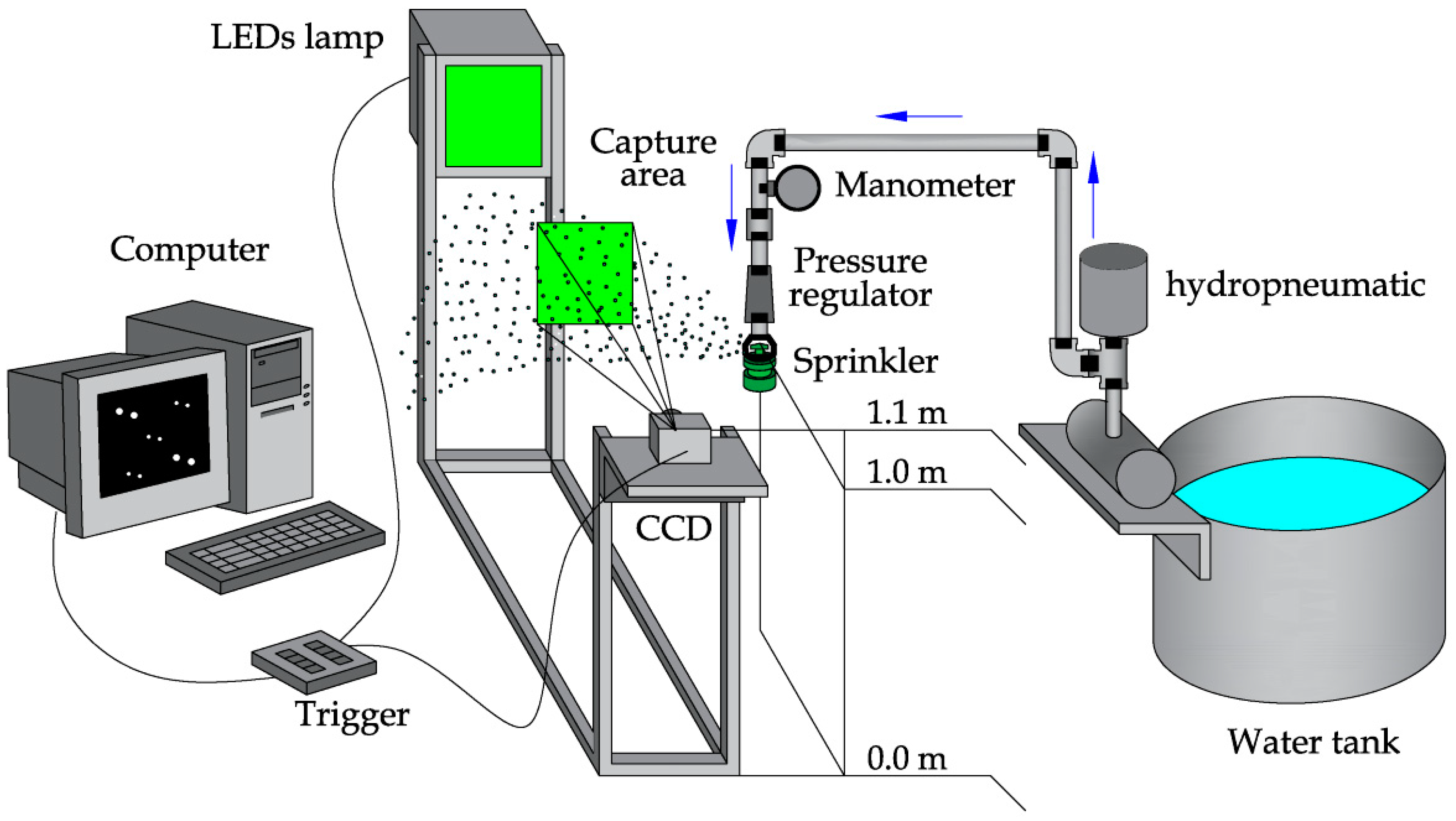
2.2. Experimental Set-Up to Characterize the Water Application Patterns

The field experiments were carried out at the facilities of the Agrifood Research and Technology Centre of Aragón located in Montañana (Zaragoza), Spain. The Nutator N3000 sprinkler was independently evaluated using a support structure to locate its deflecting plate at 2.0 m a.g.l (Figure 1a,b). The experiments were performed for the two low working pressures of 69 kPa and 103 kPa and for the nozzle sizes: 2.4, 3.8, 5.2, 6.7, 7.9, and 8.7 mm (N12, N19, N26, N34, N40 and N44, respectively). The nozzle sizes selected for this research work are commonly used in the design of the center pivot irrigation systems.

A number of devices were installed in the pipeline before the sprinkler in order to maintain the irrigation performance: (1) a sediment filter to avoid blocking the out-going jet particularly for the smaller nozzle sizes; (2) a conventional flow meter with 1 L accuracy for verifying the discharge; (3) a pressure regulator to guarantee the operating pressure of 69 kPa and 103 kPa, respectively; (4) a glycerin manometer to visually verify the pressure during each irrigation event and (5) a pressure transducer (^®Dickson) with a data logger to register the working pressure every minute (Figure 1a,b).

Flow meter readings were visually taken at the beginning and at the end of the irrigation events in order to compute the total amount of applied water. Pressure transducer data was downloaded after each irrigation event. Irrigation time was registered for each event using a conventional chronometer. The experiments were carried out while preventing the catch-cans overflow by checking the water level at different times during each event. A number of experiments were performed for each nozzle size and working pressure to evaluate the water application patterns under a range of wind velocities (calm, medium and windy) from 0.4 m s⁻¹ to 9.5 m s⁻¹.

The catch-can configuration was a square network with a 1 m side for the 4 m closest to the nozzle and a 2 m side from 4 m to 20 m from the nozzle location (Figure 1d). In order to accurately characterize the water distribution near the sprinkler, a finer catch–can network was installed close to the sprinkler where the maximum application rate was expected for this kind of sprinklers. This configuration was similar to that presented in Faci et al. [6] for the RSPS evaluations, but with reinforcement in the area surrounding the sprinkler (Figure 1d). The range of the network was increased from 20 m to 24 m in the Southeast direction due to the predominant Northwest wind direction in the area (Figure 1d). The installed network had a total of 189 catch-cans covering an area of 576 m² (Figure 1d). The catch-cans had a conical shape, with a height of 0.40 m, a total capacity of 45 mm, and they were placed at 0.05 m on the soil surface (Figure 1b). Irrigation water collected in the catch-cans was measured as soon as the irrigation was completed for each experiment. A meteorological station was installed in situ to measure the air temperature and humidity and the wind velocity and direction (Figure 1e). All meteorological variables were measured every ten seconds, and averages were recorded with a data logger every sixty seconds.

The data of each irrigation event (total amount of water applied, pressure from the data logger, irrigation collected within every catch-can and the irrigation time) were sorted in individual spreadsheets classifying the experiments according to its wind velocity per nozzle size and per operating pressure. Spatial variability in water distribution patterns was assessed using contour line maps made with the ^®SURFER software (Golden Software Inc., Golden, CO, USA) for each irrigation event.

In this research, comparisons of the irrigation performance were done with experiments under calm and windy conditions, choosing the smaller and the larger nozzle size in order to describe the radial application pattern of the Nutator sprinkler. Moreover, two radial application patterns of the Nutator sprinkler were compared with the experiments of FSPS from Ouazaa et al. [13] using the same nozzle sizes and working pressure (103 kPa).

The field data of these isolated experiments were used to calibrate the optimal parameters of the ballistic model. The simulated water distribution patterns were compared with the measured ones.

2.3. Experimental Set-Up for Drops Characterization

The Particle Tracking Velocimetry (PTV) technique of Bautista-Capetillo et al. [19] modified by Félix-Félix et al. [29] was used to characterize the sprinkler drops. The objective was to quantify the energy losses due to the impact of the jet with the sprinkler’s plate. The experiments were carried under indoor conditions at the laboratory of flow visualization of the Inter-American Institute of Technology and Water Sciences of the Autonomous University of Mexico State in Toluca, Mexico.

The experimental set-up is shown in Figure 2. The installation was composed by a pressurized irrigation system and the optical PTV system. The pressurized system was integrated by: a 0.80 m³ capacity water tank, a 0.37 kW power hydropneumatic pump and a pressure regulating tank, two 400 kPa glycerin manometers, two pressure regulators (69 kPa and 103 kPa), 22 mm PVC pipeline, and a Nutator N3000 sprinkler located at an elevation of 1 m above the soil using eight different nozzle sizes (2.0, 2.4, 3.2, 3.8, 4.4, 5.2, 6.7 and 7.9 mm corresponding to N10, N12, N16, N19, N22, N26, N34 and N40, respectively). The N40 nozzle size (7.9 mm) was not characterized with the PTV optical technique at 103 kPa due to experimental limitations affecting the pressure.

Note that the nozzle sizes used to characterize the energy losses were not the same used to characterize the application patterns. The sprinkler was surrounded with a plastic sheet for watering a minimum area, leaving a zone enough for the outgoing jet. Drop characteristics were obtained fixing the sprinkler in a position so the jets and drops came out between two frames without modifying the initial conditions of the throwing.

The PTV system with in-line volumetric illumination was integrated by an illumination system, a high-speed charge-coupled device (CCD) camera and a computer. The illumination consisted in a high-power LEDs system. The CCD camera had a temporal resolution of 250 frames per second and a spatial resolution of 1024 by 1040 pixels (the CCD pixel size was 7.4 μm) equipped with a 50 mm lens. Moreover, a synchronizer (trigger) was programed with the computer in order to control the image acquisition sequence (camera) and the light (LEDs). The particle tracking vvelocimetry sediment (PTV-SED) v2.1 algorithm from Salinas-Tapia et al. [30] was used for the image processing. Tests were performed at night, illuminating the capture zone with the LED system. Every time the camera shutter opens, the lamp is activated in two pulses originating a photograph with two groups of drops: the ones captured in the first pulse and its respective pairs in the second pulse. PTV-SED was used to obtain drops diameters, drops velocities (both horizontal and vertical components), and drops angles, taking into account the coordinates of the drop centroids and their frequency in time. With the irrigation system working, pictures were taken at a distance of 0.30 m from the sprinkler at a height of 1.10 m for characterizing the drops (Figure 2). The capture zone at each height was 0.14 m × 0.11 m.

The PTV technique could eventually identify incorrect drops pairs because of the high density of particles in an image and the high velocity of the drops (close to the initial velocity of the drops ~14 m s⁻¹ at 103 kPa). A post-processing analysis was performed in order to exclude invalid drops, so drop sizes smaller than 0.2 mm were neglected. In the first stage, the drops that do not follow a consistent behavior in their velocity and angle were rejected. Then a second filter was applied computing the inverse trajectory of the drops following the methodology of Sánchez-Burillo et al. [31]. The drops were returned to the sprinkler position using the ballistic theory with a negative time step. Drops differing 0.05 m of the sprinkler position were neglected.

Finally, the energy losses were computed for each nozzle as the difference between the theoretical velocity (Torricelli’s equation) and the volumetric averaged drop velocity after the post-processing analysis. Power regressions were obtained to predict the energy losses for a nozzle size up to 9.9 mm (# 50 of the catalog) for both operating pressures, 69 kPa and 103 kPa.

The distance of 0.30 m between the sprinkler and the capture zone was enough accurate in order to obtain the energy losses due to the jet impact with the sprinkler plate minimizing the computing time for the inverse trajectory of the drops and its error. Due to the experimental set-up, it was not possible to measure drop features at closer distances.

Further information about PTV technique and image processing could be found in Bautista-Capetillo et al. [19] and Félix-Félix et al. [29] and the research work of Sánchez-Burillo et al. [31] for the inverse simulation.

2.4. Simulation of the Water Application Patterns

2.4.1. Ballistic Simulation

Considering weight, buoyancy and drag forces; the trajectory of a spherical drop is given by:

$$\mathbf{A}=\left(1-\frac{{\rho }_a}{{\rho }_w}\right) \mathbf{g}-\frac{3{\rho }_a C^{\prime }\left|\mathbf{U}-\mathbf{W}\right|}{4{\rho }_{w}d} \left(\mathbf{U}-\mathbf{W}\right),$$

(3)

where A is the drop acceleration vector, g is the gravity vector, ρ_a and ρ_w are the air and water density, respectively, U is the drop velocity vector with respect to the ground and W is the wind velocity vector.

Among the numerical methods to solve droplet dynamics, the fourth order Runge-Kutta (RK4) with fixed time step is the most extensively used method [20,22,23,24,32]. Recently, Robles et al. [26] used the third order Runge-Kutta (RK3) with variable time step for solving the Equation (3). Establishing a maximum error of 10 cm in drops trajectories, a decrease of 8.5% in the calculation time was obtained with respect to the RK4 method. This methodology was used in this research. The following procedures regarding drops generation, drop size distributions and the calibration processes were done based on the results of Robles et al. [26].

2.4.2. Drop Size Distribution

The experiments of the isolated sprinkler under the lowest wind velocity (<1.5 m s⁻¹) for each nozzle size and working pressures were used to calibrate two volumetric drop size distributions, ULLN (Equation (4)) and Weibull (Equation (5)):

$$f\left(d\right)=\frac{\alpha \exp \left[-\frac{1}{2}{\left(\frac{\beta -\mu }{\sigma }\right)}^2\right]}{\sigma d \left(\alpha -d\right)\sqrt{2\pi }},$$

(4)

where α is the maximum drop diameter and β(d) = ln [d/(α − d)]

$$f\left(d\right)=0.693 n\frac{d^{n-1}}{d_{50}^n}\exp \left[-0.693{\left(\frac{d}{d_{50}}\right)}^n\right],$$

(5)

where f(d) is the volumetric probability density function of the total discharge from the sprinkler, d is the drop diameter, µ and σ are the mean and the standard deviation of β, respectively, and d₅₀ is the volume mean drop diameter. The ULLN distribution has three parameters α, µ and σ. The Weibull distribution has two parameters, d₅₀ and n.

The parameters of both distributions were calibrated using the free software MPCOTool [33]. This module implements a number of optimization algorithms: regular systematic sampling, Monte-Carlo, orthogonal sampling, hill climbing, and genetic algorithms. The explanation of the optimization algorithms, their delimitation, cell size and drops simulated, was described in Robles et al. [26].

After the calibration process for both distributions, the water distribution pattern was simulated with the ballistic model. The Root Mean Square Error (RMSE) and the coefficient of correlation (r) of the 189 measured and simulated pluviometries were obtained for ULLN and Weibull models. Both models were compared and one of them was selected based on the accuracy of the water distribution simulations. Relationships between the model parameters and the nozzle size were also established.

$$\mathrm{RMSE}=\frac{1}{N}\sqrt{\sum {\left(S_i-O_i\right)}^2}$$

(6)

$$\mathrm{r}=\frac{\sum \left(S_i-\overline{S}\right)\left(O_i-\overline{O}\right)}{\left(N-1\right) S{d}_s S{d}_O}$$

(7)

where N is the total pluviometries number, S_i and O_i are the simulated and observed pluviometries, respectively, $\overline{S}$ and $\overline{O}$ are the simulated and observed pluviometries averages, respectively, Sd_s and Sd_o are the standard deviations of simulated and observed pluviometries values, respectively.

2.4.3. Drag Model, Calibration and Validation

In this research, a modification of the Tarjuelo’s drag equation has been implemented. In the proposed model (L model), the K₁ and K₂ parameters of the Equation (1), are replaced with L₁·W and L₂·W, respectively:

$$C^{\prime }=C\times G,$$

(8)

where C is the Fukui’s drag coefficient; $G=\max \left(1+L_1·W·\sin \mathsf{\alpha }-L_2·W·\cos \mathsf{\beta }, 0.1\right)$; L₁ and L₂ are dimensionless parameters and $W$ is the wind velocity module (m s⁻¹), and the 0.1 constant was used in order to avoid non-physical results (negative drag resistance values).

L₁ and L₂ are now independent of the wind velocity so they can be calibrated for each group of experiments of the same nozzle size and pressure. In comparison with the Equation (1), where the K parameters are constant values during the whole trajectory of drops in one experiment, with the L model (Equation (6)), C′ can be computed with the same frequency as the measured meteorological conditions. Since the meteorology of each experiment was recorded every minute with a weather station located in situ, the C′ value changes in accordance with the measured wind conditions.

A simplification on the definition of the K parameters has been commonly practiced obtaining the drag coefficient for impact sprinklers, RSPS and FSPS [13,21,22,23,24,28]. This simplification considers the K parameters as constant values for the experiment. In this research, the meteorological variability of the experiments could be analyzed, since the L model incorporates this possibility.

For assessing the performance of the isolated very low-pressure RSPS, three different drag models were evaluated and compared based on the calibration and validation phases. The drag models assessed were (1) the proposed by Fukui et al. [20]; (2) the K coefficients according to Tarjuelo et al. [21]; and (3) the L coefficients, the model proposed on this research work. The adequacy of the simulations with the drag models 2 and 3 was compared with respect to that of model 1.

In the Fukui et al. [20] drag model, no parameters need to be calibrated since drop drag coefficient is determined by its size and its velocity. The RMSE of this model was computed in every experiment for both pressures between the 189 measured and simulated pluviometries, and compared with the RMSE of the calibration and the validation processes of the other drag models.

The parameters of the Tarjuelo’s drag model were calibrated for each individual experiment of the isolated sprinkler for both pressures. In contrast, the parameters of the new model L were calibrated by nozzle size groups and working pressure. Calibrating each individual experiment could introduce an overfitting problem and the failure to predict experiments with different conditions. On the other hand, calibrating the parameters by groups represents an advantage for generalizing the model and minimizing the errors with less probability to overfit [34].

The validation phase was based on the leaving-one-out-cross validation (LOOCV) method. In LOOCV only one experiment is selected as the validation set and the rest of the experiments are used to calibrate. The process is repeated to validate every experiment. In the Tarjuelo’s model, a linear interpolation between the closest points is used to estimate the coefficients of the validation case. In the L model, the constant parameters of the group calibration are introduced in the validation case. The predicted ability of both models was assessed in terms of RMSE (between measured and simulated irrigations) and r in the validation phase.

3. Results and Discussion

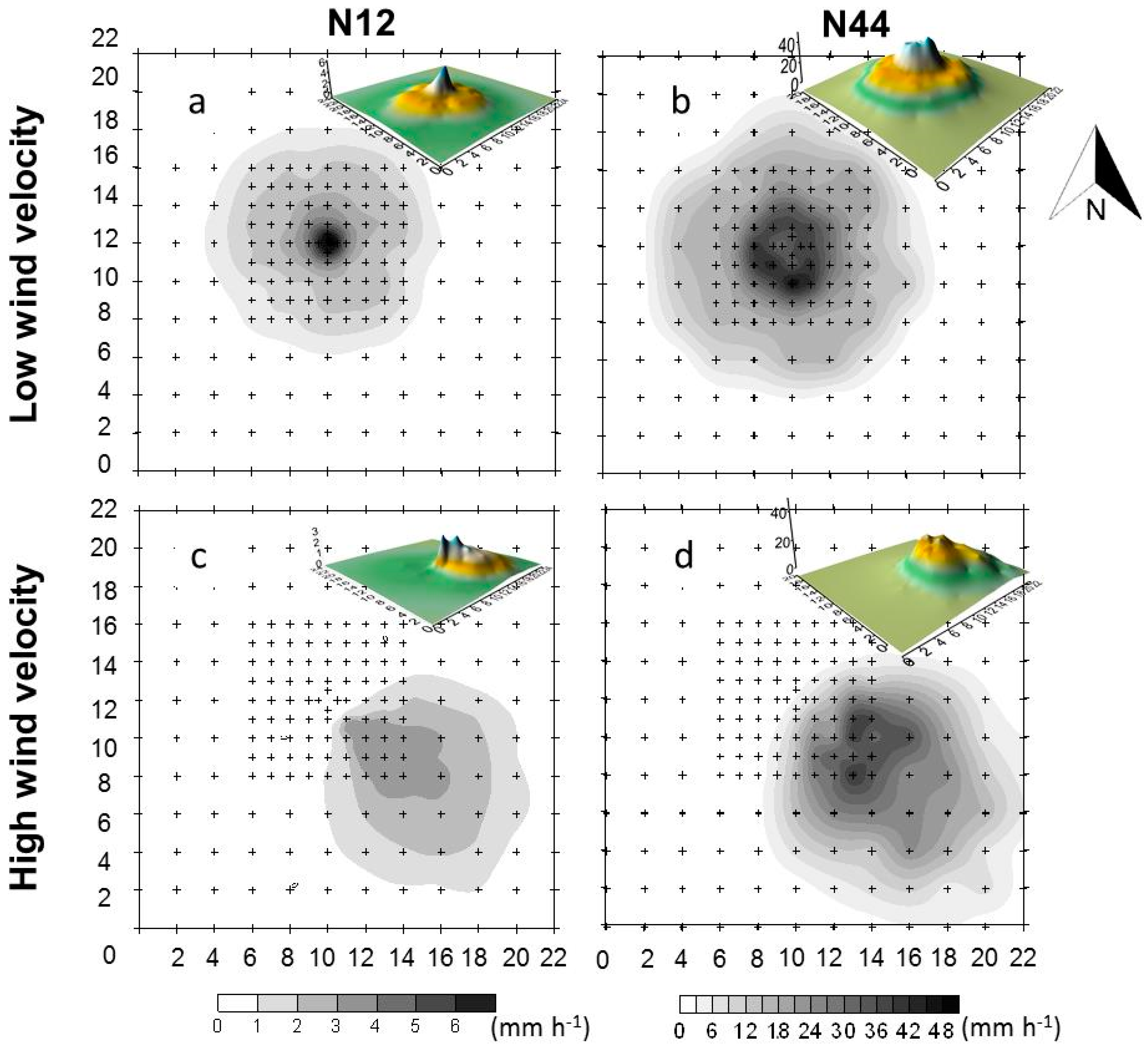
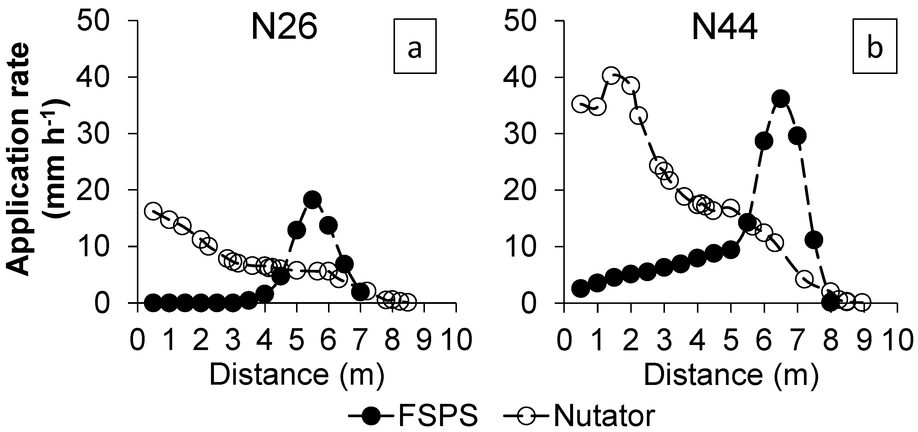
3.1. Water Application Patterns

Table 1. Experimental features of the measurements of the isolated Nutator sprinkler.

Nozzle Size (mm)	69 kPa				103 kPa
	Exp +	Wind Velocity (m s−1)	Irrigation Time (h)	Pressure SD (kPa) ψ	Exp +	Wind Velocity (m s−1)	Irrigation Time (h)	Pressure SD (kPa) ψ
2.4	4	1.1–6.9	1.8–3.0	0.4	6	0.7–8.3	2.8–3.4	0.7
3.8	5	1.6–6.1	1.8–3.0	0.7	6	0.9–6.1	2.1–3.1	1.0
5.2	5	1.3–7.7	1.0–2.8	0.4	6	0.4–9.4	1.5–2.1	0.7
6.7	4	0.9–7.4	1.0–1.9	0.5	5	0.8–8.5	1.0–1.1	0.8
7.9	7	0.9–5.7	1.0–1.3	0.5	6	0.6–8.2	1.0–1.1	0.9
8.7	8	1.2–7.6	1.0–1.4	0.5	4	0.6–9.7	1.0	0.9

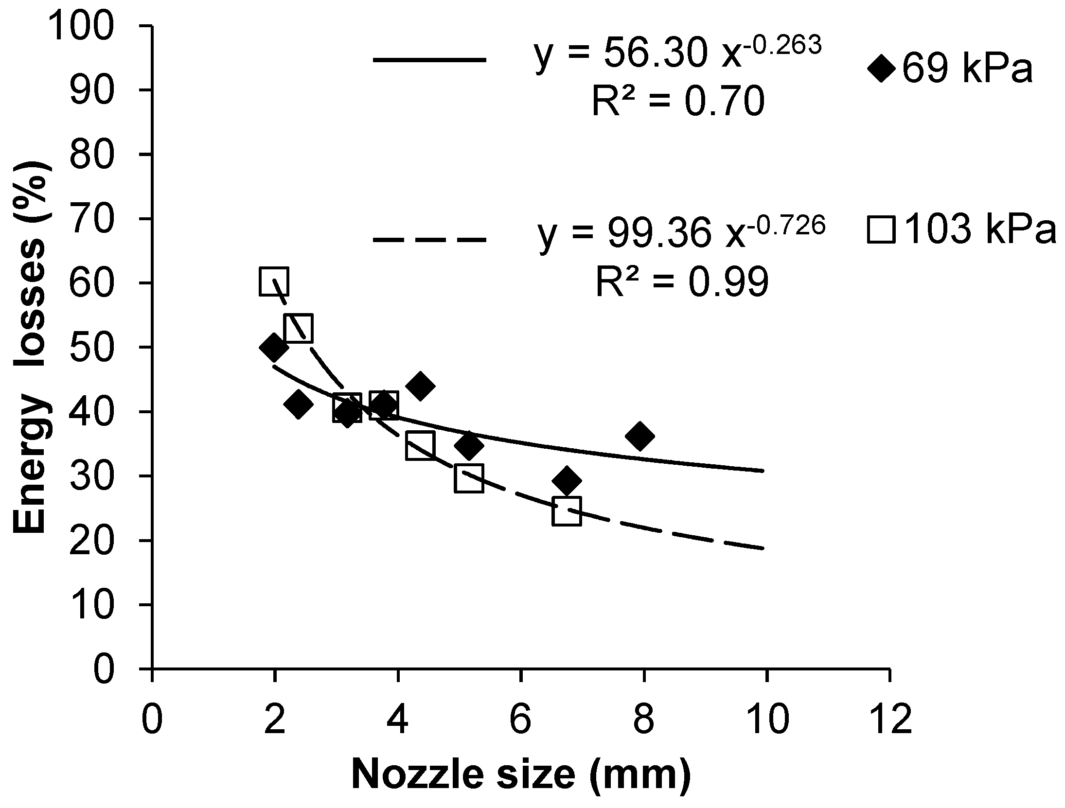
^ψ mean standard deviation-SD-of the pressure measured with the pressure data logger per nozzle size experiment. ⁺ Number of experiments per nozzle size for both operating pressures.

shows the features of the water application pattern experiments performed on the isolated sprinkler plot. The wind velocity range of the experiments was between 0.6 m s⁻¹ and 9.7 m s⁻¹. A total of 33 tests for both operating pressures (69 kPa and 103 kPa) and 7447 pluviometer readings were performed during two evaluation seasons. The experiments under the working pressure of 69 kPa were conducted in 2016 (between May–September) while the ones for 103 kPa were carried out between October–December 2017 and January-February 2018. An average of 5 experiments per nozzle size and operating pressures were evaluated, covering calm, medium, and high wind conditions.

The average wind velocity of the experiments at 103 kPa was higher than those for 69 kPa (Table 1). Maximum wind velocities of 7.7 m s⁻¹ and 9.7 m s⁻¹ were registered for both operating pressures and minimum wind velocities of 0.9 m s⁻¹ and 0.6 m s⁻¹ were observed for 69 kPa and 103 kPa, respectively. Depending on the nozzle size and working pressure, the experiments lasted from a minimum of 1 h to a maximum of 3.4 h. The operating pressure along the irrigation events registered with the Dickson datalogger, suggests small variations in the out-going flow in each nozzle size, which indicates a correct operation of the pressure regulators. The maximum standard deviation-SD-observed was 0.7 kPa and 0.9 kPa for 69 kPa and 103 kPa, respectively. That barely represents 1% for each operating pressure.

The Figure 3 shows illustrative examples of the measured individual water distributions patterns at 103 kPa with the nozzle N12 (Figure 3a,c) and nozzle N44 (Figure 3b,d) under calm and windy conditions. The water application rate (mm h⁻¹) is shown in gray scale for each experiment (note that the scale color is different between nozzle sizes). The maximum application rate measured on the N12 nozzle was 6.4 mm h⁻¹ and 3.3 mm h⁻¹ for calm and windy conditions, respectively. While the maximum irrigation measured on the N44 was 41 mm h⁻¹ and 25 mm h⁻¹ for calm and windy conditions, respectively. These differences on irrigation between the two wind velocity intensities could be due to the variations in the wind velocity and in the wind direction that distort the pluviometry pattern. Moreover, the wind and drift evaporation losses (not evaluated in this work) and to the sampling variance because of low pluviometers density at measurements with high wind velocities modify the maximum application rates. Under low wind velocity, the wetted diameter by the N12 and N44 nozzle sizes reaches up to 14 m and 18 m, respectively. The experiments with low wind velocity (Figure 3a,b) were performed at 1 m s^–1, the experiment at high wind velocity for N12 nozzle was 6 m s⁻¹ (Figure 3c) and the scenario of N44 nozzle (Figure 3d) was performed at 9 m s⁻¹.

Table 2. Experimental features of isolated sprinklers under low wind conditions.

Pressure (kPa)	Nozzle Size (mm)	Measured Volume (L h−1)	Wetted Radii (m)	Maximum Application Rate (mm h−1)	r
69	2.4	130.5	6.5	2.2	0.93
	3.8	418.0	8.7	5.9	0.93
	5.2	816.0	8.6	10.0	0.98
	6.7	1366.7	8.4	17.3	0.97
	7.9	1927.9	8.4	25.3	0.97
	8.7	2295.7	9.0	30.0	0.97
103	2.4	209.2	7.6	6.4	0.87
	3.8	560.4	8.6	10.2	0.94
	5.2	1053.0	8.6	16.2	0.96
	6.7	1701.3	9.2	24.0	0.98
	7.9	2445.6	9.2	32.2	0.98
	8.7	2901.0	9.9	40.3	0.97

shows the experimental features of the isolated Nutator sprinkler at the two pressures under low wind conditions. The irrigation volume collected from the pluviometers and the wetted radii (obtained from the boundary pluviometers wetted in each event) are also shown in the Table 2. The maximum application rate for all the experiments occurred between 0.0 m and 1.5 m from the sprinkler location. Under low-wind conditions, the radial application pattern (cross section of the spatial distribution pattern) for all nozzle sizes and both pressures were triangular in shape. The correlation coefficients (r) shown in the Table 2 represent the relationship between the application rate and the distance from the sprinkler. The r values suggest that the radial application becomes more triangular as the nozzle size and the operating pressure increases.

The triangular shape of the Nutator sprinkler is similar to the impact sprinklers commonly used in solid-set systems, but different from the fixed spray plate sprinklers such as the FSPS (with a doughnut/ring-shape). Figure 4 shows a comparison of the radial application patterns performed on two different nozzle sizes with a Nutator sprinkler (used in this research) and a FSPS at the same operating pressure of 103 kPa under no wind conditions. The data of the FSPS was obtained from Ouazaa et al. [13]. The nozzles compared were N26 (5.2 mm) (Figure 4a) and N44 (8.7 mm) (Figure 4b). According to Christiansen [35], theoretically, the triangular shape of the radial application, as the one of the Nutator sprinkler, could produce the most uniform distribution at overlapping the water distribution patterns of the emitters integrating the irrigation machine. There is a difference of 1.5 m in the wetted radii between the two sprinklers for the N26 nozzle and a difference of 1.0 m for the N44 nozzle, with the largest irrigated area for the Nutator sprinkler. This could be explained by a number of factors of each sprinkler FSPS and Nutator at 103 kPa, such as: drop sizes, deflecting plate geometry, jet break-up and therefore, the energy losses.

On the other hand, the radial application pattern of the Nutator sprinkler is similar to the one of Ouazaa et al. [13] using a RSPS model R3000 ^®Nelson (red plate with 6 grooves). The main difference between R3000 sprinkler and the Nutator is that the first requires pressures from 138 kPa, while the Nutator can operate from 69 kPa.

3.2. Energy Losses

Table 3. Drop features as arithmetic average values defined with the PTV technique after the post-processing for 69 kPa and 103 kPa, and for each of the nozzle sizes analyzed.

Pressure (kPa)	Nozzle Size (mm)	Number of Drops Analyzed	Drop Diameter (mm)	Drop Velocity (m s−1)	Drop Angle (°)
69	2.0	220	1.1	7.3	17.8
	2.4	187	1.1	7.6	17.6
	3.2	470	1.1	7.5	18.0
	3.8	345	1.2	7.7	17.5
	4.4	1058	1.0	7.1	18.2
	5.2	751	0.9	8.2	18.3
	6.7	629	1.0	9.0	17.7
	7.9	1053	1.0	8.9	18.2
103	2.0	180	0.9	7.8	17.1
	2.4	542	1.0	8.8	17.0
	3.2	326	1.1	9.3	17.2
	3.8	636	1.1	9.7	17.1
	4.4	538	1.0	10.0	17.5
	5.2	710	1.1	10.5	17.4
	6.7	1909	0.9	10.8	17.4

shows the drops features obtained with the PTV technique for each nozzle size and for both pressures. For the pressure of 69 kPa, a total of 10,227 droplets were analyzed from which about 53% (5514 drops) were neglected after the post-processing, leaving 4713 valid drops. For this pressure, the arithmetic average of drop diameter, the minimum and the maximum drop diameters reached values of 1.0 mm, 0.2 mm, and 4.0 mm, respectively. The arithmetic average velocity of the drops at 69 kPa was 8.0 m s⁻¹ with a standard deviation of 2.4 m s⁻¹. The drops flew with an arithmetic average angle of 18° with respect to the horizontal plane.

For a pressure of 103 kPa, a total of 6475 droplets were analyzed and about 25% (1634) of them were removed after the filtering, remaining 4841 valid drops (see Table 3). Values of the average drops diameter, the minimum and the maximum drop diameters of 1.0 mm, 0.2 mm and 4.8 mm were obtained, respectively. At 103 kPa, the drops flew to an average of 2.0 m s⁻¹ faster than at 69 kPa (average drops velocity 10 m s⁻¹) with a standard deviation of 3.0 m s⁻¹. The average outgoing angle of the drops was 1° lower than for the pressure of 69 kPa (average drops angle of 17° with respect to the horizontal plane).

A considerably large drops number (~17,000) was analyzed with the semiautomatic PTV technique [19,29] compared with the labor-intensive low-speed photographic technique [13,18] where hundreds of drops are commonly characterized.

The radial velocity component of the drops ranged between 7.1 m s⁻¹ and 10.8 m s⁻¹. Then, the tangential velocity component is between 1.8% and 2.7% of the total velocity. These values have been considered as negligible for PTV drop measurements and also for drop ballistic simulation. There are another uncertainty sources as sprinkler vibrations, pressure fluctuations, advection streams, etc. that, as the tangential velocity, has been also neglected. The Figure 5 shows the relationships between drop diameter and drop velocity for the pressures of 69 kPa (Figure 5a,b) and 103 kPa (Figure 5c,d) for two nozzle sizes N10 (2.0 mm) and N34 (6.7 mm). In general, for the Nutator sprinkler some particularities are noticeable: the drops velocity increases with nozzle size and the operating pressure, the drop diameters increases with the nozzle size (up to 4.8 mm) and finally, a large number of small drops are generated for the larger nozzle sizes (from nozzle N26-5.2 mm onwards) with a wide velocities range for both pressures. The variability on drop velocity for the small drops in large nozzle sizes (from N26) are due to the high uncertainty of the inverse trajectory resolution (small drops subjected to high drag).

The energy losses of the RSPS presented in Figure 6 were calculated with the volumetric averaged drop velocity for each nozzle size and operating pressure shown in Figure 5. The energy losses decrease with the nozzle size. Power regressions between nozzle size and energy losses relationships were stablished for both operating pressures. For the pressure tests of 69 kPa, minimum losses of 29% and maximum of 50% were observed and for the experiments of 103 kPa, the energy losses ranged between 19% and 60%.

The energy losses observed of the Nutator sprinkler of this research work can be compared with those obtained by other authors using fixed spray plate sprinklers (FSPS). Ouazaa et al. [13] found higher energy losses for FSPS working at 69 kPa with respect to the Nutator sprinkler (from 40% to 70%) using the low-speed photographic technique to characterize the drops of five nozzle sizes between 2.4 mm and 6.7 mm. Zhang et al. [14], using an optical technique (PTV) to characterize the drops of a FSPS, obtained energy losses ranging between 28% and 50% for a pressure of 100 kPa using a 4.8 mm nozzle size. Sánchez-Burillo et al. [31] used the photographic technique of Salvador et al. [18] and, after returning the drops to its initial position found energy losses between 33% and 74% using a FSPS with an operating pressure of 138 kPa for the nozzles 3.75 mm, 6.75 mm and 7.97 mm.

In agreement with Ouazaa et al. [13] and Zhang et al. [14] and the results of this research, sprinkler design should be reviewed for FSPS and for the RSPS included the Nutator sprinklers to minimize the energy losses, mainly for the smaller nozzle sizes.

3.3. Ballistic Model

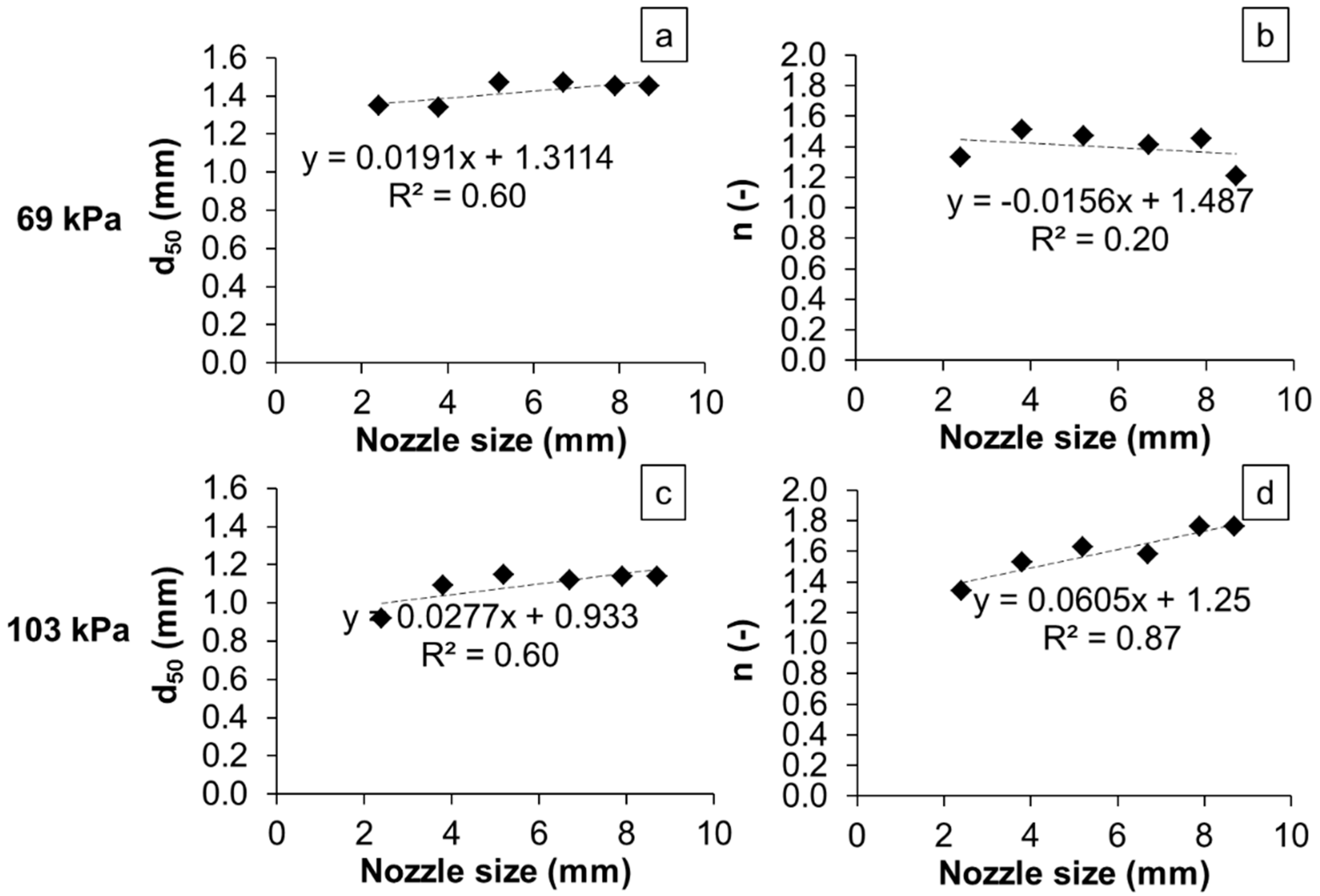
3.3.1. Drop Size Distribution

A total of six experiments (one per nozzle size) of the isolated Nutator sprinkler under low wind conditions (<1.5 m s⁻¹) were selected to calibrate the parameters of both drop size distributions (Weibull and ULLN) for both operating pressures.

A comparison of both drop size distributions is shown in Figure 7, assessing the RMSE between the measured and simulated pluviometries of the six experiments. Each relationship is presented with a different symbol for each pressure. The 1:1 line is also represented in the figure. Although a slightly higher RMSE was observed using the Weibull model for both pressures, the statistical difference between ULLN and Weibull RMSE’s is not significant at the 95.0% confidence level. Based on previous comparisons and considering the computational costs, a Weibull drop size distribution was selected to simulate the water application patterns of the experiments.

Table 4. Optimal parameters of Weibull drop size distribution model for both operating pressures and nozzle sizes.

Pressure (kPa)	Nozzle Size (mm)	d50 (mm)	n	Application Rate (mm h−1)	RMSE (mm h−1)	R
69	2.4	1.35	1.33	0.99	0.21	0.96
	3.8	1.34	1.51	1.75	0.75	0.93
	5.2	1.47	1.47	3.51	0.84	0.97
	6.7	1.47	1.41	6.21	1.45	0.96
	7.9	1.45	1.45	8.76	2.10	0.97
	8.7	1.45	1.21	11.3	2.70	0.98
103	2.4	0.92	1.34	1.14	0.37	0.95
	3.8	1.09	1.53	2.41	0.74	0.96
	5.2	1.15	1.63	4.52	0.80	0.99
	6.7	1.12	1.58	6.43	1.26	0.99
	7.9	1.14	1.76	9.25	2.22	0.98
	8.7	1.14	1.76	11.5	3.10	0.97

shows the optimal parameters of the Weibull distribution (d₅₀ and n) for both operating pressures and for each nozzle size evaluated. The RMSE increases with the nozzle size. The maximum RMSE was found for 8.7 mm nozzle size, with 2.7 mm h⁻¹ and 3.1 mm h⁻¹ for pressures of 69 kPa and 103 kPa, respectively. According to our measurements, the maximum RMSE reaches 24% and 27% of the total amount of water applied in one hour for 69 kPa and 103 kPa, respectively, RMSE increases with the nozzle flow. The Weibull model presents good adjustments, with correlation coefficients between 0.93 and 0.99.

The relationship between the nozzle size and the Weibull model parameters was presented in Figure 8. A linear regression was adjusted between nozzle sizes and the parameters d₅₀ and n, for the pressure of 69 kPa (Figure 8a,b) and for the pressure of 103 kPa (Figure 8c,d). As expected, the tendency of d₅₀ is to increase with the nozzle size, because larger nozzle generates larger drops, and to decrease with the working pressure. The average values of d₅₀ were 1.42 mm and 1.10 mm for 69 kPa and 103 kPa, respectively. There is a significant statistical difference between the values of n for the two working pressures at the 95.0% confidence level after a Fisher’s least significant difference (LSD) procedure. Average values of 1.4 and 1.6 were found for n at 69 kPa and 103 kPa, respectively. Kincaid et al. [16] and Ouazaa [13] working with RSPS, obtained a similar relationship between the model parameters, d₅₀ and n, and the nozzle size and working pressure.

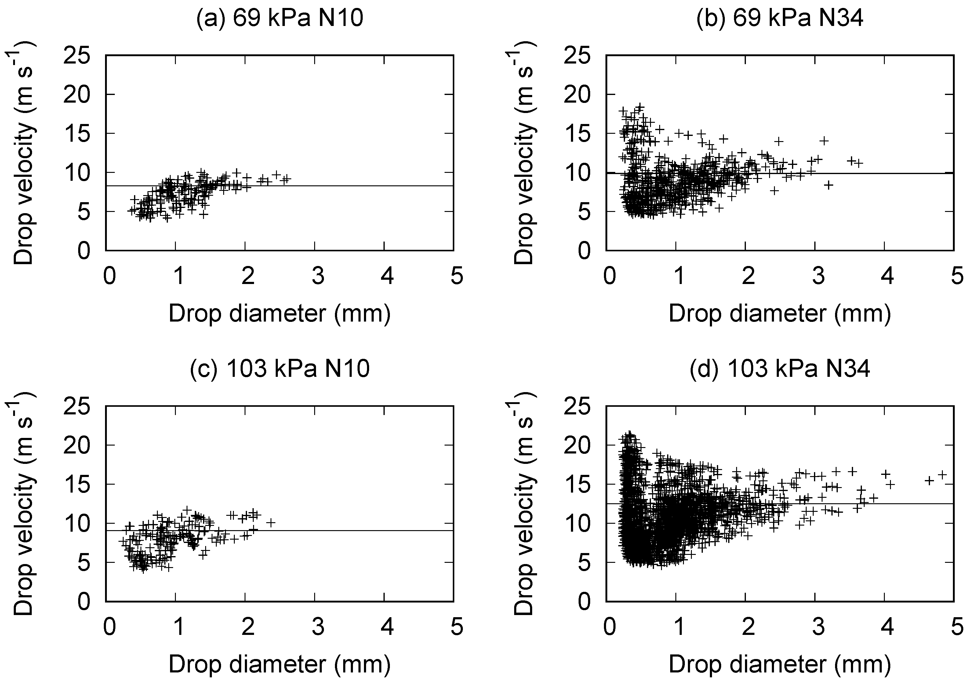
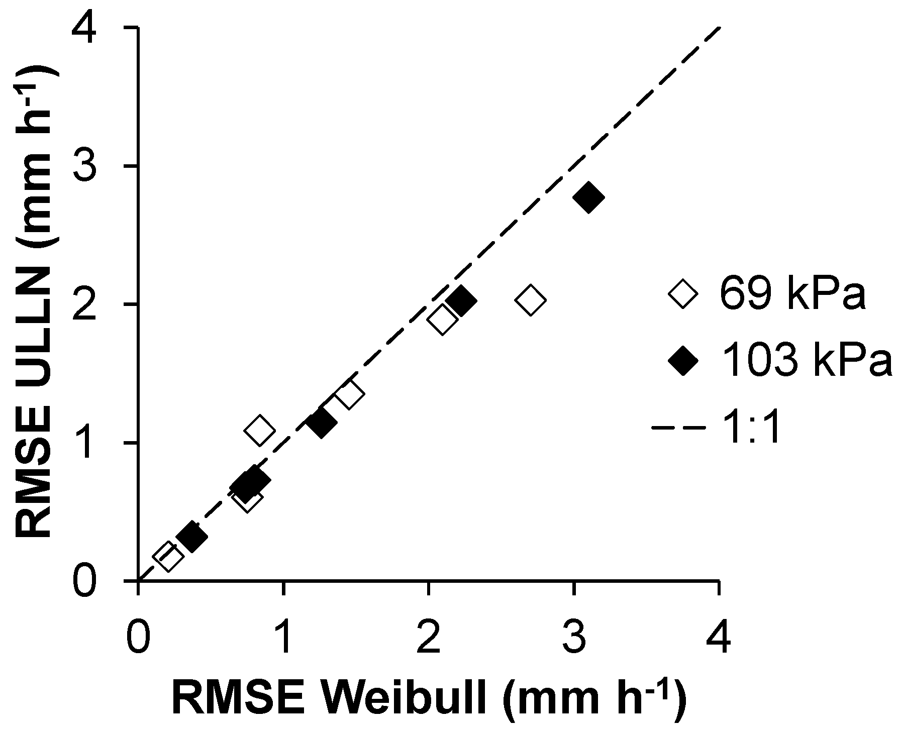
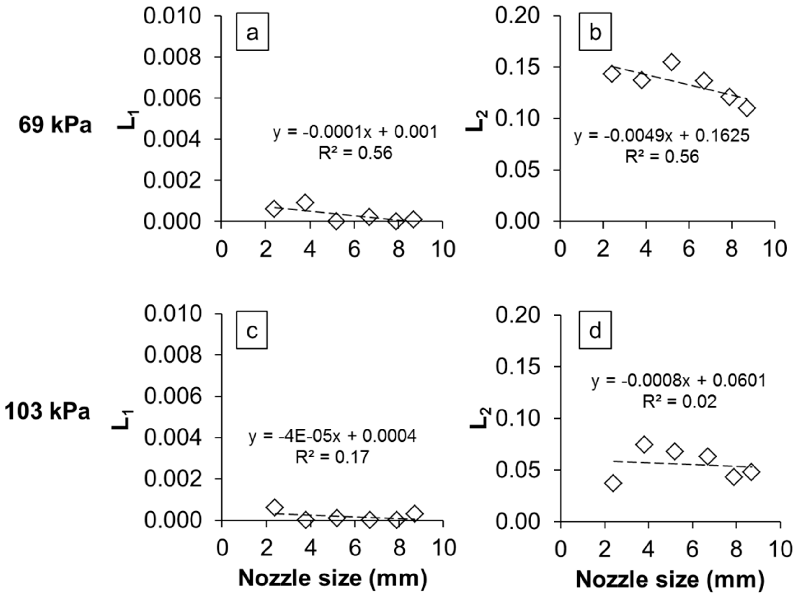
3.3.2. Drag Coefficient, Calibration and Validation

In the calibration phase, the RMSE using the model of Fukui et al. [20] was related with the models of Tarjuelo et al. [21] and L for both pressures (Figure 9a,b). The three models accurately simulated the experimental measurements. The values of RMSE for the three models ranged between 0.18 mm h⁻¹ and 5.10 mm h⁻¹ for the pressure of 69 kPa, while for the pressure of 103 kPa the range was 0.3 mm h⁻¹ to 6.2 mm h⁻¹. There was not statistically significant difference between the RMSE of the three models for both pressures. For the pressure of 69 kPa the RMSE of the L model were slightly lower compared with the Fukui et al. [20] model. Figure 9b (103 kPa) shows more variability of the RMSE’s between the three models compared with the lowest pressure of 69 kPa (Figure 9a). For both pressures, the largest RMSE were obtained for the larger nozzle sizes (8.7 mm) using any model and the highest errors are associated with the high wind velocities (>5 m s⁻¹) and with the higher water application rate of the large nozzles. For the pressure of 69 kPa, the maximums RMSE were 4.5 mm h⁻¹ (K model), 4.6 mm h⁻¹ (L model) and 5.1 mm h⁻¹ (Fukui’s model), representing 28%, 30% and 32%, respectively, of the water application rate for the 8.7 mm nozzle size. For a pressure of 103 kPa, the maximums RMSE were 5.1 mm h⁻¹ (K model), 5.2 mm h⁻¹ (L model) and 6.2 mm h⁻¹ (Fukui’s model), representing 22%, 27% and 30%, respectively, of the water application rate for the 8.7 mm nozzle size. The computational time for the calibrations and the validations were similar for both models K and L, 5 days and 5 h for the L model, and 5 days and 7 h for the K model.

Although no significant differences were observed between the three models in the calibration phase, slightly larger differences were found in validation. The LOOCV methodology of the validation phase used the 33 experiments performed for both pressures 69 kPa (Figure 9c) and 103 kPa (Figure 9d). The assessment in validation phase is more relevant, since the blind simulation represents the performance of a model in a real scenario under unknown conditions. There is not significant statistical difference on the RMSE of the Fukui et al. [20] model and the K model for both pressures at 95.0% confidence level. However, for the pressure of 103 kPa, three simulations had a higher RMSE using the K model. The largest RMSE of the validation phase corresponds to the 8.7 mm nozzle size experiments, with values of 5.4 mm h⁻¹ for the K model and 3.1 mm h⁻¹ for the L and Fukui’s models. These differences represent 24% (K model) and 13% (with L model and Fukui’s model) of the total amount of water applied in one hour.

Moreover, there is no statistically significant difference between both RMSE of the Fukui et al. [20] model and the L model for both pressures at 95.0% confidence level in the validation phase. However, slightly higher RMSE’s were observed using the Fukui et al. [20] model with respect to the L model for 31 cases in the pressure of 69 kPa and for 24 cases for the pressure of 103 kPa. The maximum RMSE, 6.2 mm h⁻¹, was found for the 8.7 mm nozzle size working at 103 kPa using Fukui’s model which represents 29% of the total amount of water applied. For the same pressure of 103 kPa, the maximum RMSE value with the L model is 5.7 mm h⁻¹, which represents 25% of the total amount of water applied in one hour.

The worst cases reproduced in the validation phase with the K model (Figure 9d), were under wind velocities lower than 1 m s⁻¹, which indicate a failure in the model of Tarjuelo et al. [21] at null wind velocities. It is common to establish the K parameters as zero but the threshold is not clear. On the other hand, the L model has a natural transition to Fukui’s model.

In summary, at the validation phase and under the worst scenario, the L model improves the irrigation performance on 11% with respect to the K model and 4% respect to the Fukui et al. [20] model.

Figure 10 shows the relationship between nozzle size and the parameters L₁ and L₂ for a working pressure of 69 kPa (Figure 10a,b) and for a working pressure of 103 kPa (Figure 10c,d). The resulting linear regression models showed that there is not a clear effect of the operating pressure on the values of the L₁ parameters. Moreover, the optimal values of the parameters L₁ for both pressures can be considered as zero (Figure 10a,c). As the L₂ values increase, the drag coefficient of the drops decreases. The values of the parameter L₂ decrease as the nozzle size increases for the low pressure (Figure 10b). For the 103 kPa working pressure, the relationship between nozzle size and L₂ parameter is very weak; therefore it can be considered as a constant with an average value of 0.06. The previous recommendations given for the Nutator sprinkler used in this research could differ in values and/or tendencies for other sprinklers as RSPS or FSPS.

4. Conclusions

The experimental characterization of a low-pressure rotator spray plate sprinkler was performed covering a wide range of meteorological conditions, nozzle sizes, and working pressures.

The radial application pattern of the Nutator sprinkler was triangular shape ensuring and adequate distribution uniformity of the overlapped sprinklers. The reported technical data of the isolated sprinkler under low wind conditions could be useful for designing center pivot irrigations systems.

The PTV technique allowed us to measure the features of 16,702 droplets originated from the sprinkler that were post-processed in order to obtain reliable data for energy losses characterization. This semiautomatic technique represents an advantage in the number of drops analyzed vs. calculation time with respect to the low-speed photographic technique. Moreover, the PTV technique was adequate to estimate the energy losses of the Nutator sprinklers, which ranged from 19% to 60%.

ULLN drop size distribution reproduced accurately the water application pattern of the RSPS at low pressure as much as the Weibull model, while the latter model was selected for simplicity and to save computational cost.

The properties of the L model proposed in this work represent an advantage over the previous models by improving the drops physics, and generalize its use for unknown conditions and new irrigation material. The new proposed model improves the calibration/validation processes by improving the nozzle size and pressure groups (avoiding overfitting), the drag force definition that is computed within a variable meteorology, and the continuous transition of the L model to the Fukui’s model for low wind velocities.

At the validation phase, the L model in the Nutator sprinkler resulted in lower errors than the K model (28%). The K model was not accurate enough for this kind of sprinklers, even compared with the simple drag ballistic model of Fukui without corrections by the wind. The L model also resulted in slightly lower errors than the Fukui’s drag model (4%).

Five regressions per operating pressure were proposed (energy losses, d₅₀, n, L₁ and L₂) in order to obtain the parameters model for the non-evaluated nozzle sizes in between the minimum (2.4 mm) and the maximum (8.7 mm) evaluated.

The L drag model proposed in this research represents an opportunity to reproduce the irrigation of other spray plate sprinklers, RSPS and FSPS. Further work is necessary in order to assess the improved model for impact sprinklers.

References

1. Keller, J.; Bliesner, R.D. Sprinkle and Trickle Irrigation; Van Nostrand Reinhold: New York, NY, USA, 1991. [Google Scholar]
2. Tarjuelo, J.M. El Riego por Aspersión y su Tecnología, 3rd ed.; Ediciones Mundi-Prensa: Madrid, España, 1999. [Google Scholar]
3. Playán, E.; Garrido, S.; Faci, J.M.; Galán, A. Characterizing pivot sprinklers using an experimental irrigation machine. Agric. Water Manag. 2004, 70, 177–193. [Google Scholar] [CrossRef] [Green Version]
4. ESYRCE. Encuesta de Superficies y Rendimientos de Cultivos en España; Ministerio de Agricultura Pesca y Alimentación: Madrid, España, 2017; p. 101.
5. National Agricultural Statistics Service (USDA). 2014 Census of Agriculture. Farm and Ranch Irrigation Survey; USDA: Washington, DC, USA, 2013; Volume 3, pp. 100–103.
6. Faci, J.M.; Salvador, R.; Playán, E.; Sourell, H. A comparison of fixed and rotating spray plate sprinklers. J. Irrig. Drain. Eng. ASCE 2001, 127, 224–233. [Google Scholar] [CrossRef]
7. Moreno, M.A.; Ortega, J.F.; Córcoles, J.I.; Martínez, A.; Tarjuelo, J.M. Energy analysis of irrigation delivery systems: Monitoring and evaluation of proposed measures for improving energy efficiency. Irrig. Sci. 2010, 28, 445–460. [Google Scholar] [CrossRef]
8. Tarjuelo, J.M.; Rodríguez-Díaz, J.A.; Abadía, R.; Camacho, E.; Rocamora, C.; Moreno, M.A. Efficient water and energy use in irrigation modernization: Lessons from Spanish case studies. Agric. Water Manag. 2015, 162, 67–77. [Google Scholar] [CrossRef]
9. Mugele, R.A.; Evans, H.D. Droplet size distribution in sprays. Ind. Eng. Chem. 1951, 43, 1317–1324. [Google Scholar] [CrossRef]
10. Solomon, K.H.; Kincaid, D.C.; Bezdek, J.C. Drop size distribution for irrigation spray nozzles. Trans. ASAE 1985, 28, 1966–1974. [Google Scholar] [CrossRef]
11. Molle, B.; Le Gat, Y. Model of water application under pivot sprinkler: II. Calibration and results. J. Irrig. Drain. Eng. 2000, 126, 348–354. [Google Scholar] [CrossRef]
12. Legat, Y.; Molle, B. Model of water application under pivot sprinkler. 1: Theoretical grounds. J. Irrig. Drain. Eng. 2000, 126, 343–347. [Google Scholar]
13. Ouazaa, S.; Burguete, J.; Paniagua, P.; Salvador, R.; Zapata, N. Simulating water distribution patterns for fixed spray plate sprinkler using the ballistic theory. Span. J. Agric. Res. 2014, 12, 850–863. [Google Scholar] [CrossRef] [Green Version]
14. Zhang, Y.; Sun, B.; Fang, H.; Zhu, D.; Yang, L.; Li, Z. Experimental and simulation investigation on the kinetic energy dissipation rate of a fixed Spray-plate sprinkler. Water 2018, 10, 1365. [Google Scholar] [CrossRef]
15. Li, J.; Kawano, H.; Yu, K. Droplet size distributions from different shaped sprinkler nozzles. Trans. ASAE 1994, 37, 1871–1878. [Google Scholar] [CrossRef]
16. Kincaid, D.C.; Solomon, K.H.; Oliphant, J.C. Drop size distributions for irrigation sprinklers. Trans. ASAE 1996, 39, 839–845. [Google Scholar] [CrossRef]
17. Montero, J.; Tarjuelo, J.M.; Carrión, P. Sprinkler droplet size distribution measured with an optical spectropluviometer. Irrig. Sci. 2003, 22, 47–56. [Google Scholar] [CrossRef]
18. Salvador, R.; Bautista-Capetillo, C.; Burguete, J.; Zapata, N.; Playán, E. A photographic method for drop characterization in agricultural sprinklers. Irrig. Sci. 2009, 27, 307–317. [Google Scholar] [CrossRef]
19. Bautista-Capetillo, C.; Robles, O.; Salinas-Tapia, H.; Playán, E. A particle tracking velocimetry technique for drop characterization in agricultural sprinklers. Irrig. Sci. 2014, 32, 437–447. [Google Scholar] [CrossRef] [Green Version]
20. Fukui, Y.; Nakanishi, K.; Okamura, S. Computer evaluation of sprinkler irrigation uniformity. Irrig. Sci. 1980, 2, 23–32. [Google Scholar] [CrossRef]
21. Tarjuelo, J.M.; Carrión, P.; Valiente, M. Simulación de la distribución del riego por aspersión en condiciones de viento. Investig. Agrar. Prod. Prot. Veg. 1994, 9, 255–272. [Google Scholar]
22. Carrión, P.; Tarjuelo, J.M.; Montero, J. SIRIAS: A simulation model for sprinkler irrigation: I. Description of the model. Irrig. Sci. 2001, 20, 73–84. [Google Scholar] [CrossRef]
23. Dechmi, F.; Playán, E.; Cavero, J.; Faci, J.M.; Martínez-Cob, A. Wind effects on solid set sprinkler irrigation depth and yield of maize (Zea mays). Irrig. Sci. 2003, 22, 67–77. [Google Scholar] [CrossRef]
24. Playán, E.; Zapata, N.; Faci, J.M.; Tolosa, D.; Lacueva, J.L.; Pelegrín, J.; Salvador, R.; Sánchez, I.; Lafita, A. Assessing sprinkler irrigation uniformity using a ballistic simulation model. Agric. Water Manag. 2006, 84, 89–100. [Google Scholar] [CrossRef] [Green Version]
25. Zerihun, D.; Sanchez, C.A.; Warrick, A.W. Sprinkler irrigation droplet dynamics. I: Review and theoretical development. J. Irrig. Drain. Eng. 2016, 142, 04016007. [Google Scholar] [CrossRef]
26. Robles, O.; Latorre, B.; Zapata, N.; Burguete, J. Self-calibrated ballistic model for sprinkler irrigation with a field experiments data base. Agric. Water Manag. 2019, in press. [Google Scholar] [CrossRef]
27. Seginer, I.; Nir, D.; von Bernuth, D. Simulation of wind distorted sprinkler patterns. J. Irrig. Drain. Eng. ASCE 1991, 117, 285–306. [Google Scholar] [CrossRef]
28. Ouazaa, S. Development of Models for Solid-Set and Center-Pivot Sprinkler Irrigation Systems. Ph.D. Thesis, University of Zaragoza, Zaragoza, Spain, July 2015. Available online: http://digital.csic.es/handle/10261/117636 (accessed on 10 February 2019).
29. Félix-Félix, J.R.; Salinas-Tapia, H.; Bautista-Capetillo, C.; García-Aragón, J.; Burguete, J.; Playán, E. A modified particle tracking velocimetry technique to characterize sprinkler irrigation drops. Irrig. Sci. 2017, 35, 515–531. [Google Scholar] [CrossRef]
30. Salinas-Tapia, H.; García, A.J.; Moreno, H.D.; Barrientos, G.B. Particle tracking velocimetry (PTV) algorithm for non-uniform and nonspherical particles. In Proceedings of the Electronics, Robotics and Automotive Mechanics Conference CERMA, Cuernavaca, México, 26–29 September 2006; Volume 2, pp. 322–327. [Google Scholar]
31. Sánchez-Burillo, G.; Delirhasannia, R.; Playán, E.; Paniagua, P.; Latorre, B.; Burguete, J. Initial drop velocity in a fixed spray plate sprinkler. J. Irrig. Drain. Eng. 2013, 139, 521–531. [Google Scholar] [CrossRef]
32. Vories, E.D.; Von Bernuth, R.D.; Mickelson, R.H. Simulating sprinkler performance in wind. J. Irrig. Drain. Eng. 1987, 113, 119–130. [Google Scholar] [CrossRef]
33. GitHub. MPCOTool: The Multi-Purposes Calibration and Optimization Tool. By Burguete, J. and Latorre, B.. Available online: http://github.com/jburguete/mpcotool (accessed on 9 January 2019).
34. Burnham, K.P.; Anderson, D.R. Model Selection and Multimodel Inference, 2nd ed.; Springer: New York, NY, USA, 2002; p. 488. [Google Scholar]
35. Christiansen, J.E. Irrigation by Sprinkling; Bulletin 670; University of California, College of Agriculture, Agricultural Experiment Station: Berkeley, CA, USA, 1942; p. 124. [Google Scholar]
Figure 1. Experimental set-up for the characterization of the water application patterns of the Nutator sprinkler: (a) isolated Nutator sprinkler and its components (pressure regulators, manometer and pressure transducer); (b) field experimental layout; (c) Nutator sprinkler; (d) experimental catch-can set-up; (e) meteorological weather station.
Water 11 01684 g001
Figure 2. Experimental set-up for drops characterization. Spacings and components of the hydraulic and optical systems are shown.
Water 11 01684 g002
Figure 3. Measured water distribution at 103 kPa for the nozzle N12 (2.4 mm) and nozzle N44 (8.7 mm) for calm conditions (a,b) and windy conditions (c,d).
Water 11 01684 g003
Figure 4. Measured radial water application at 103 kPa for (a) the nozzle N26 (5.2 mm) and (b) nozzle N44 (8.7 mm) of the Nutator sprinkler and FSPS (from Ouazaa et al. [13]).
Water 11 01684 g004
Figure 5. Measured drop diameter vs. measured drop velocity obtained with the PTV optical technique for the pressures of 69 kPa (a,b) and 103 kPa (c,d) (nozzle sizes N10-2.0 mm and N34-6.7 mm are shown). The continuous horizontal line represents the volumetric average drops velocity for each nozzle size and pressure.
Water 11 01684 g005
Figure 6. Estimated energy losses as function of the nozzle size. Energy loss regressions are shown for both pressures 103 kPa and 69 kPa with different symbols.
Water 11 01684 g006
Figure 7. Comparisons of both drop size distributions, ULLN and Weibull, for 103 kPa and 69 kPa. Both operating pressures are represented with a different symbol. The dashed line represents the 1:1 relationship.
Water 11 01684 g007
Figure 8. Optimal parameters of Weibull drop size distribution model (d50 and n) for both operating pressures 69 kPa (a,b) and 103 kPa (c,d). The dashed line represents the linear regression for each case.
Water 11 01684 g008
Figure 9. RMSE comparisons of the calibration (a,b) and validation (c,d) phases for the operating pressures of 69 kPa and 103 kPa. RMSE of the Fukui et al. [20] drag model vs. RMSE of the L model and Tarjuelo et al. [21] drag model for both pressures are shown in each figure. Each model is shown with a different symbol. The 1:1 relationship is represented with a dashed line.
Water 11 01684 g009
Figure 10. Optimal values of the L model related to the nozzle size for both operating pressures 69 kPa (a,b) and 103 kPa (c,d). Linear regressions are shown for each parameter.
Water 11 01684 g010