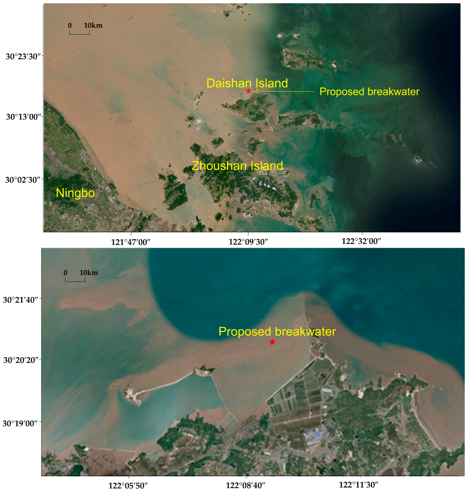
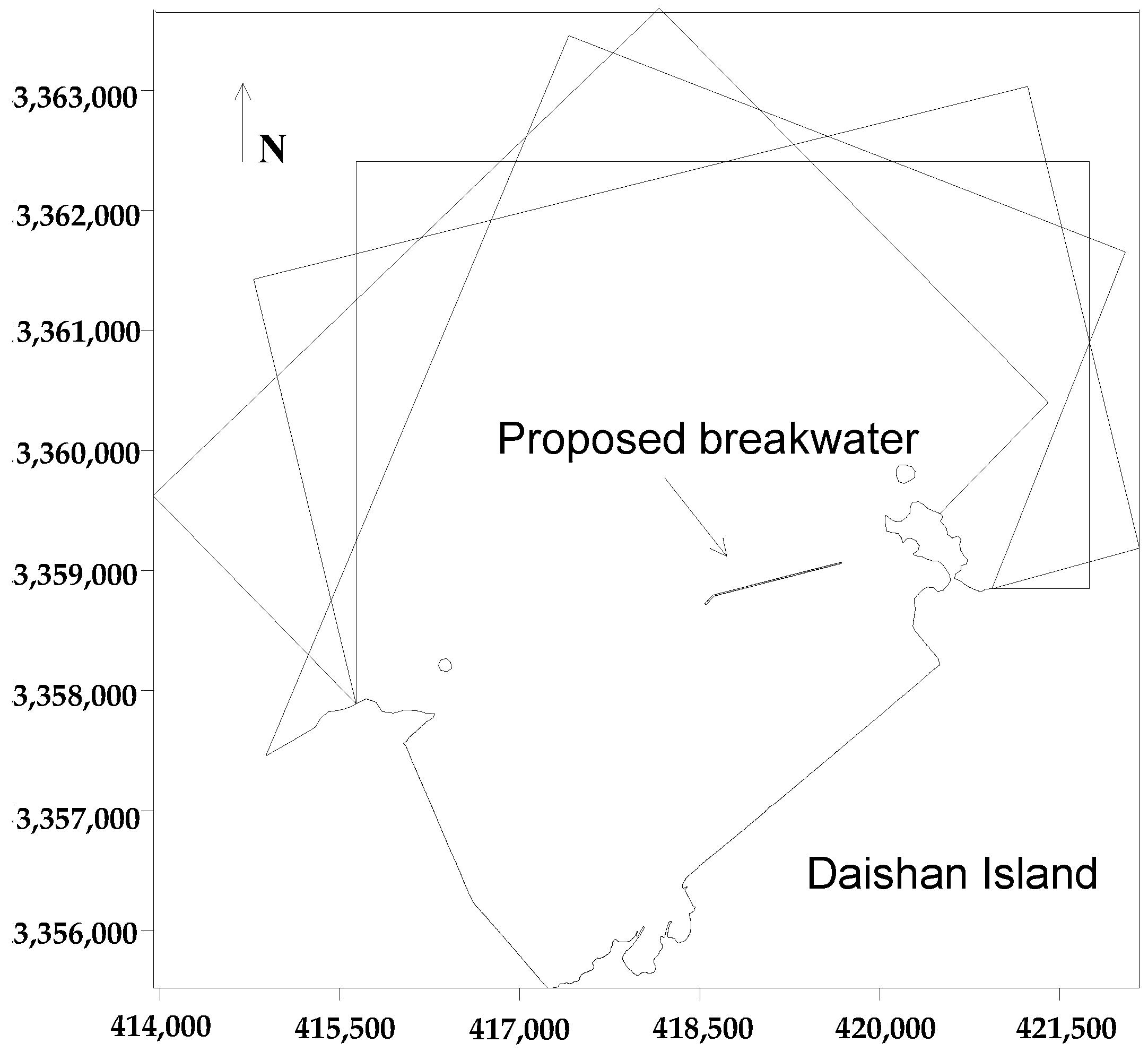
Figure 1.
Geographic environment in survey region.
Figure 1.
Geographic environment in survey region.
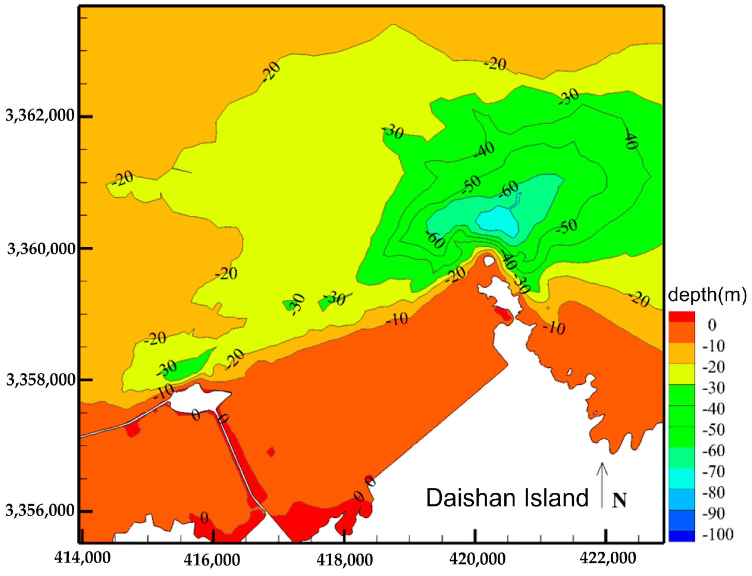
Figure 2.
Underwater topographic map of the engineering area.
Figure 2.
Underwater topographic map of the engineering area.
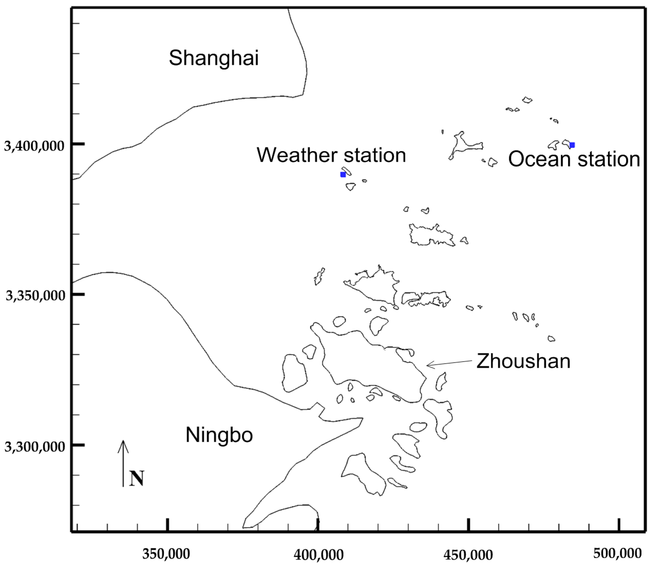
Figure 3.
Position of observation stations.
Figure 3.
Position of observation stations.
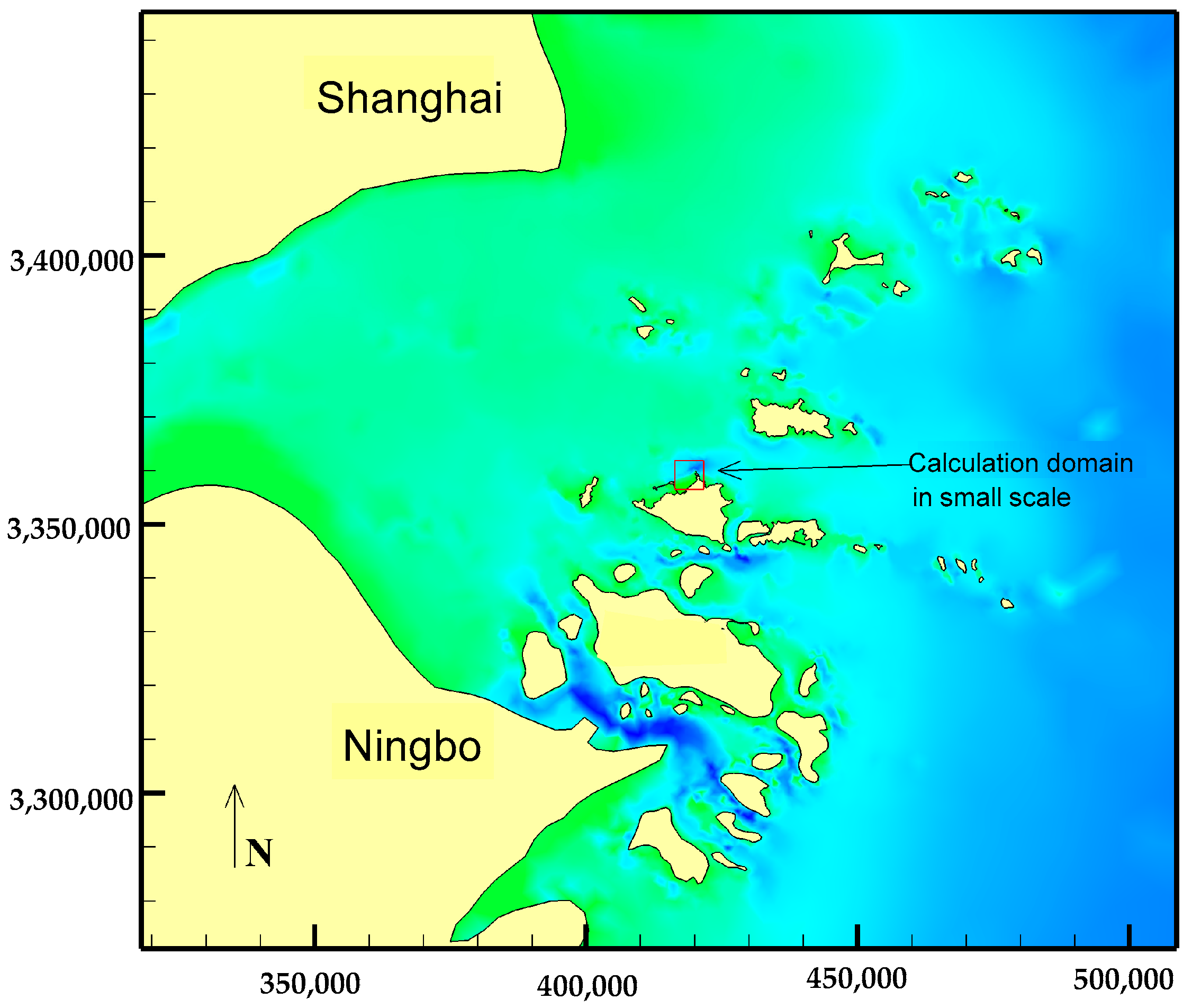
Figure 4.
Calculation domain of the surface water (SW) model.
Figure 4.
Calculation domain of the surface water (SW) model.
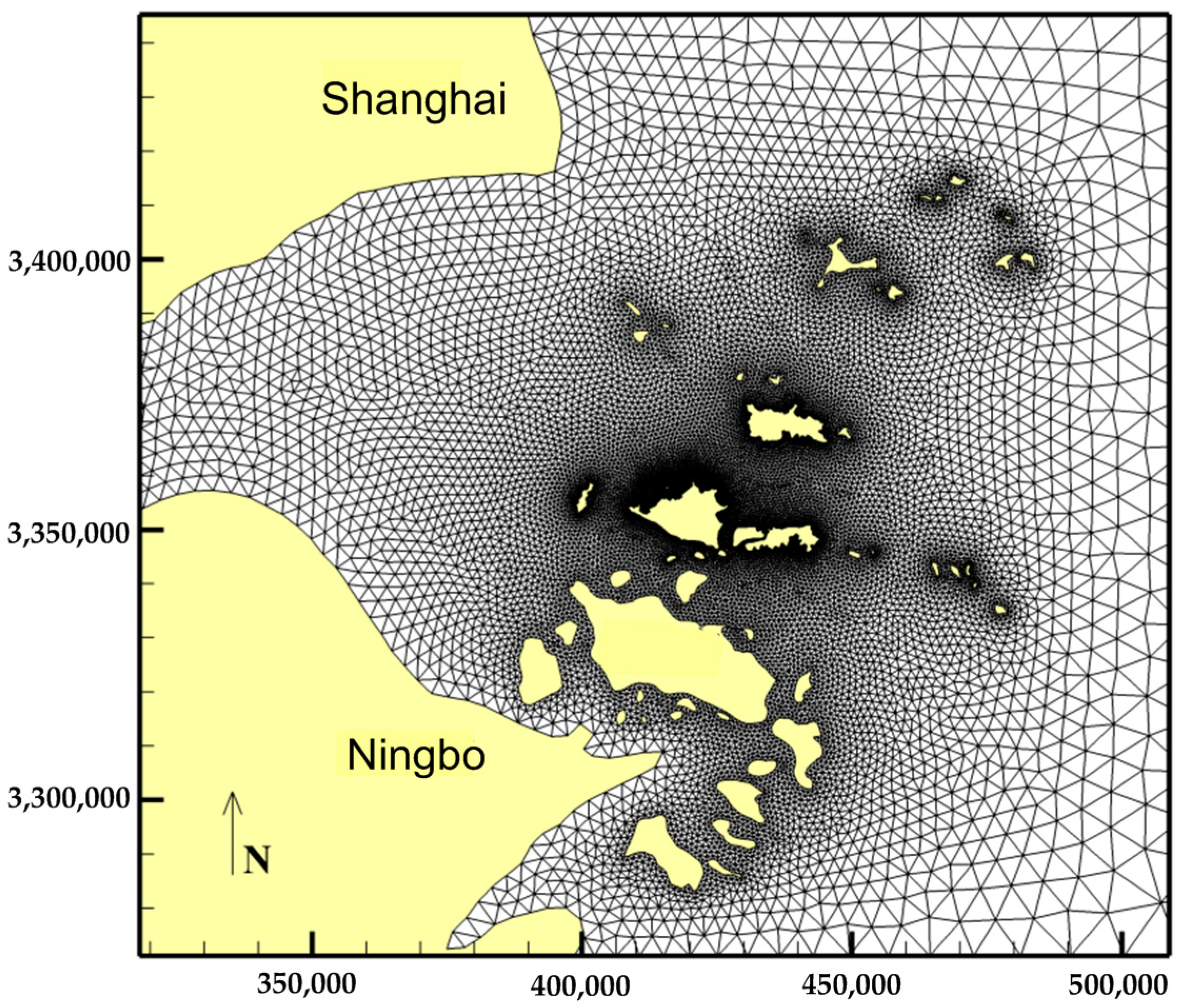
Figure 5.
Grid division of SW model.
Figure 5.
Grid division of SW model.
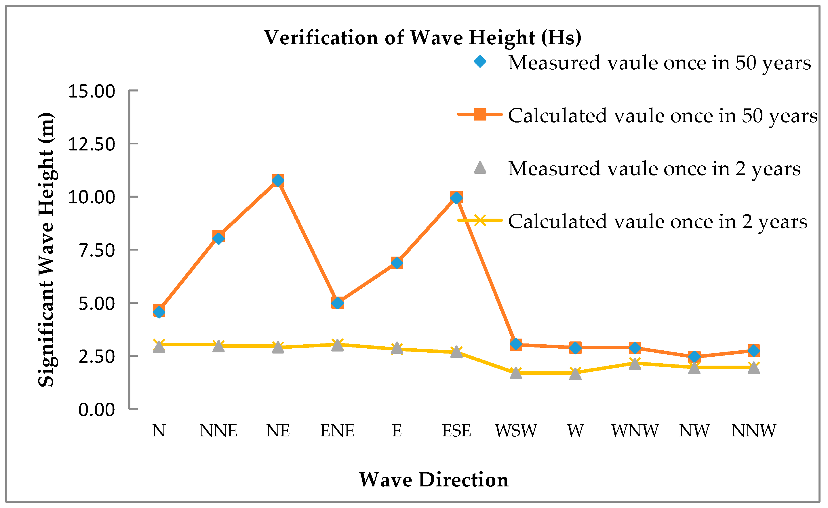
Figure 6.
Verification chart of significant wave height (Hs).
Figure 6.
Verification chart of significant wave height (Hs).
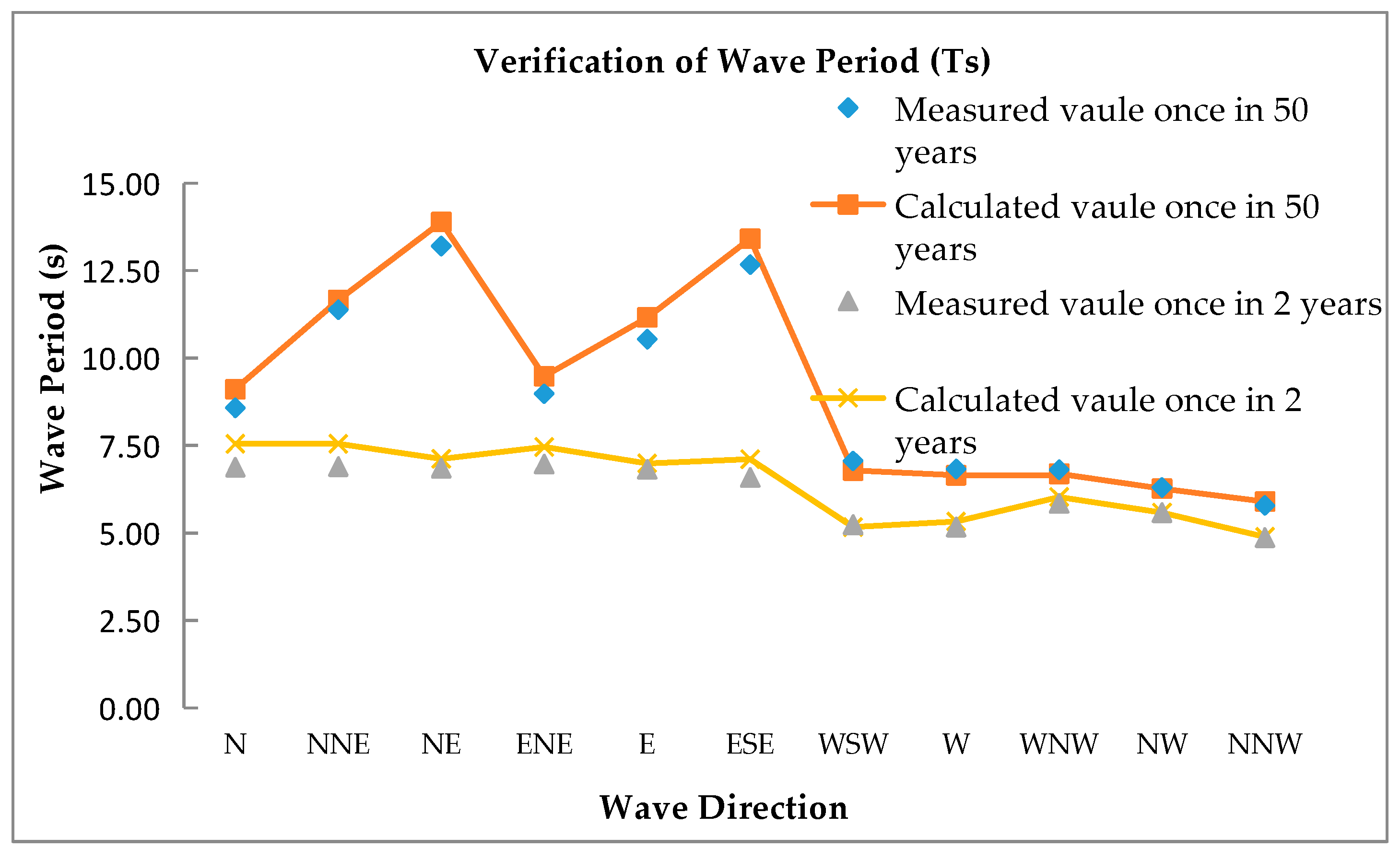
Figure 7.
Verification chart of significant period (Ts).
Figure 7.
Verification chart of significant period (Ts).
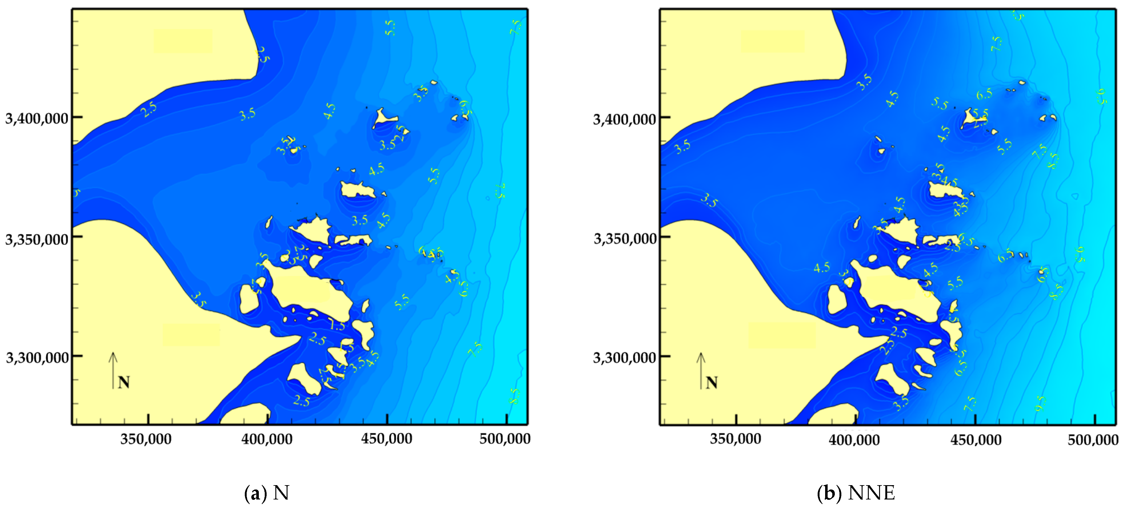
Figure 8.
Distribution of significant wave height on a large scale before engineering.
Figure 8.
Distribution of significant wave height on a large scale before engineering.
Figure 9.
Schematic diagram of different wave directions in the computational domain.
Figure 9.
Schematic diagram of different wave directions in the computational domain.
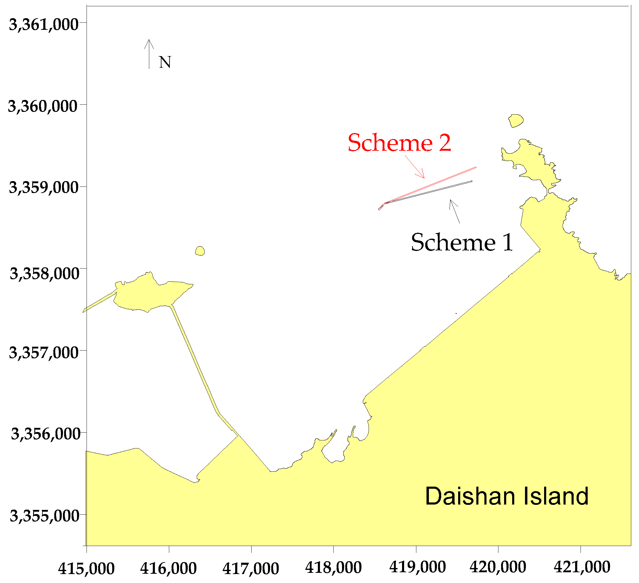
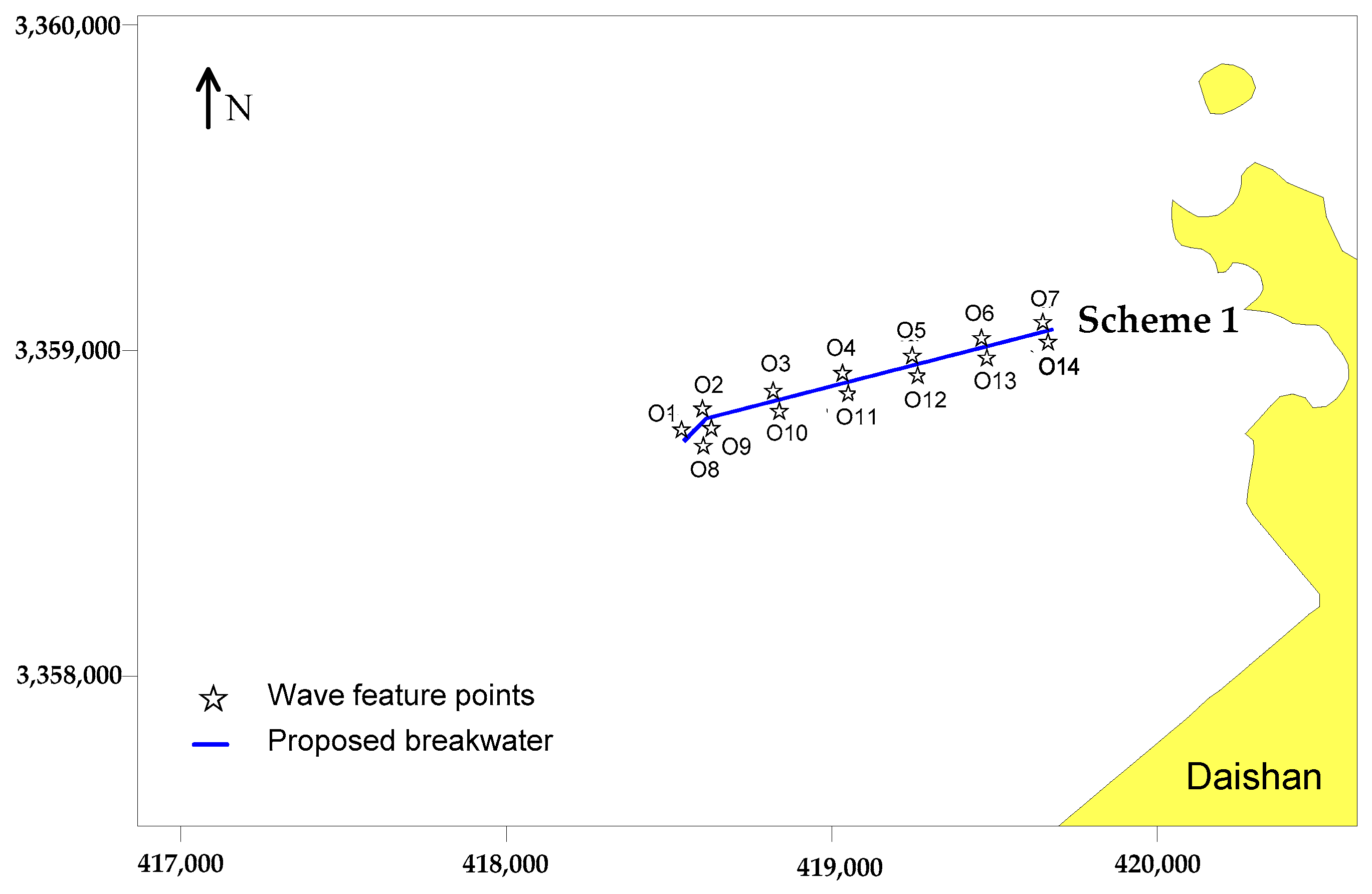
Figure 10.
Layout of the breakwater.
Figure 10.
Layout of the breakwater.
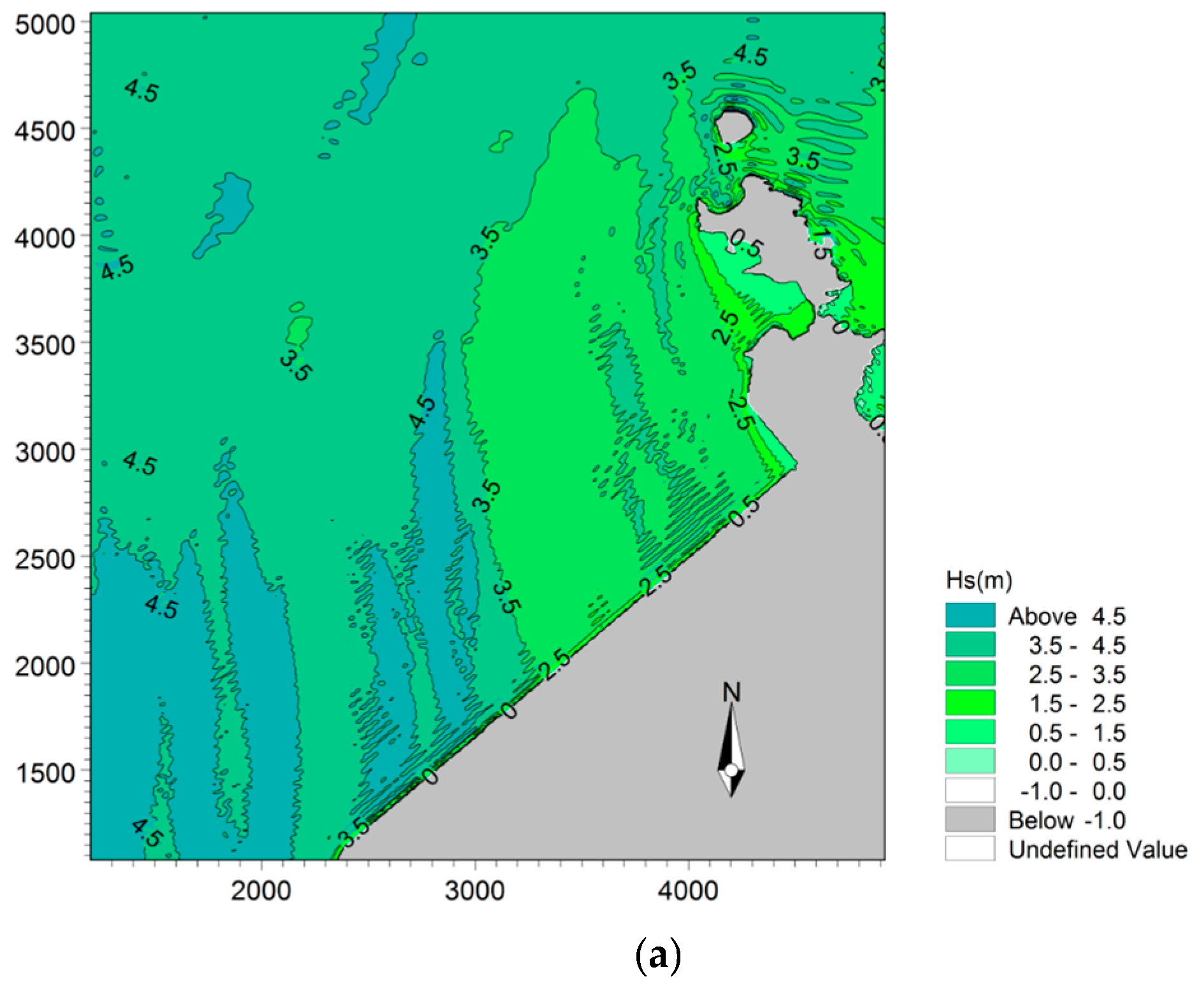
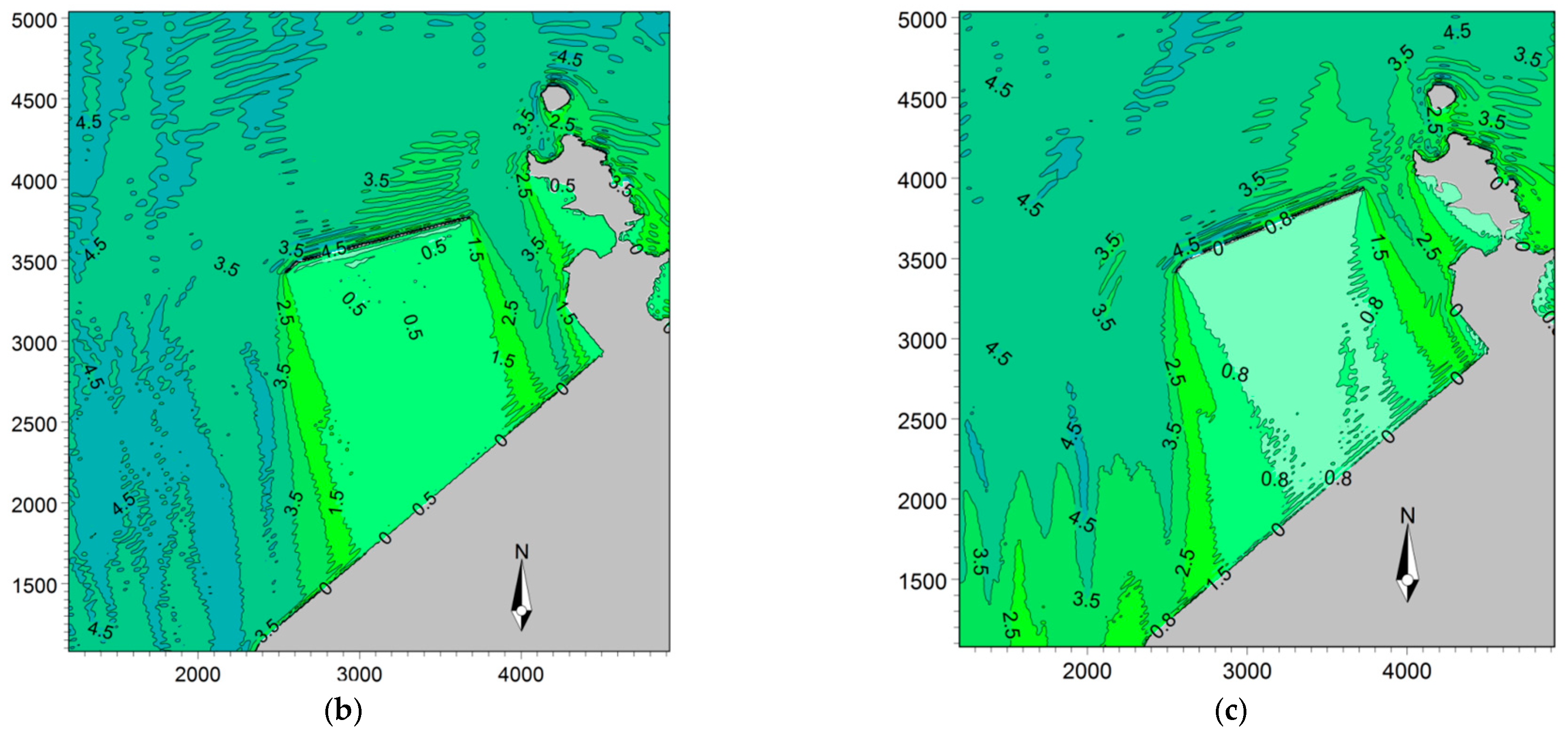
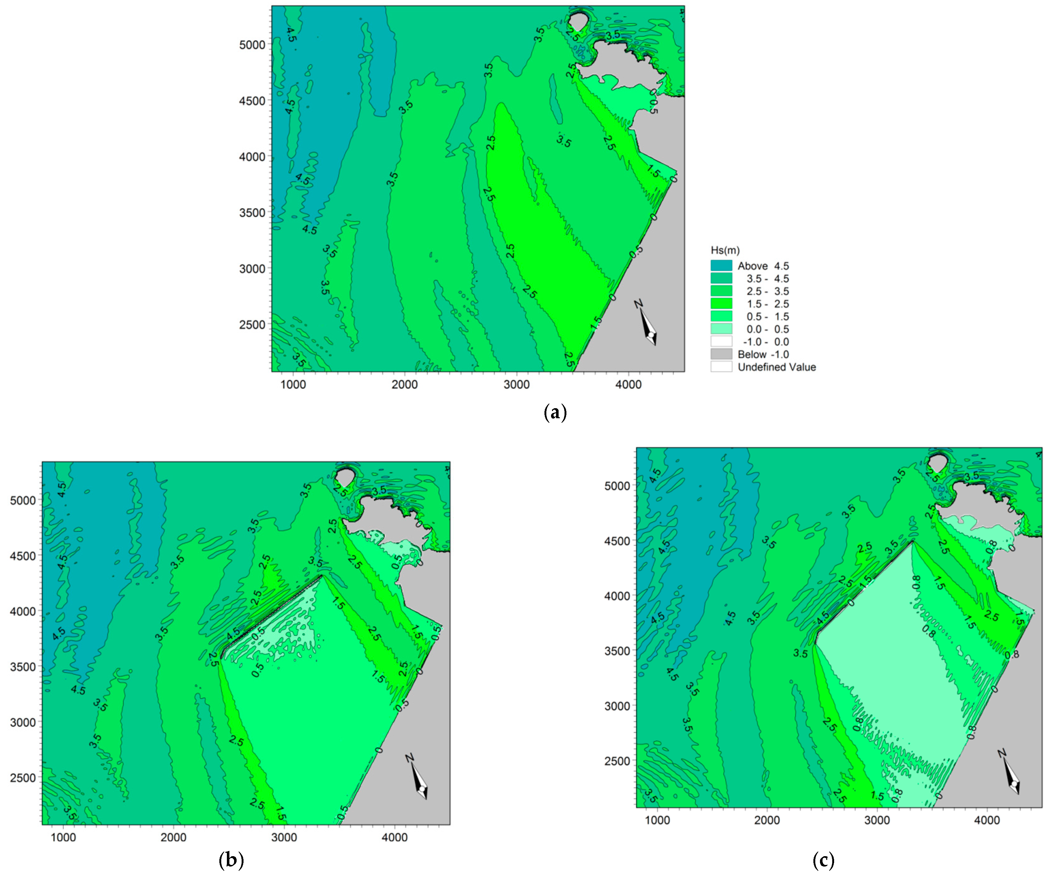
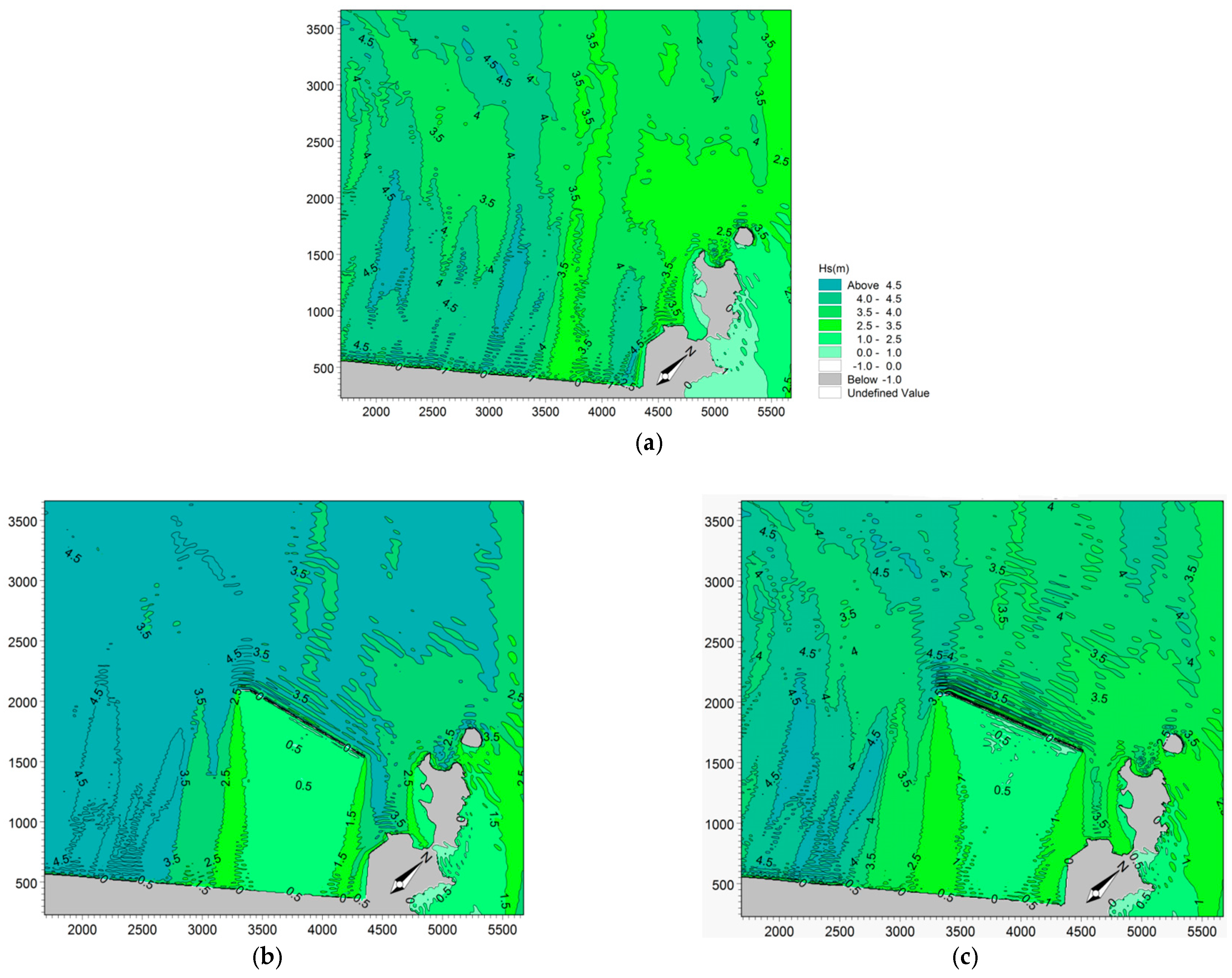
Figure 11.
Distribution of significant wave height in the N direction under three working conditions: (a) before the project, (b) Scheme 1, (c) Scheme 2. Notes: In the figure, wave height vaules and plane coordinates are all in meters.
Figure 11.
Distribution of significant wave height in the N direction under three working conditions: (a) before the project, (b) Scheme 1, (c) Scheme 2. Notes: In the figure, wave height vaules and plane coordinates are all in meters.
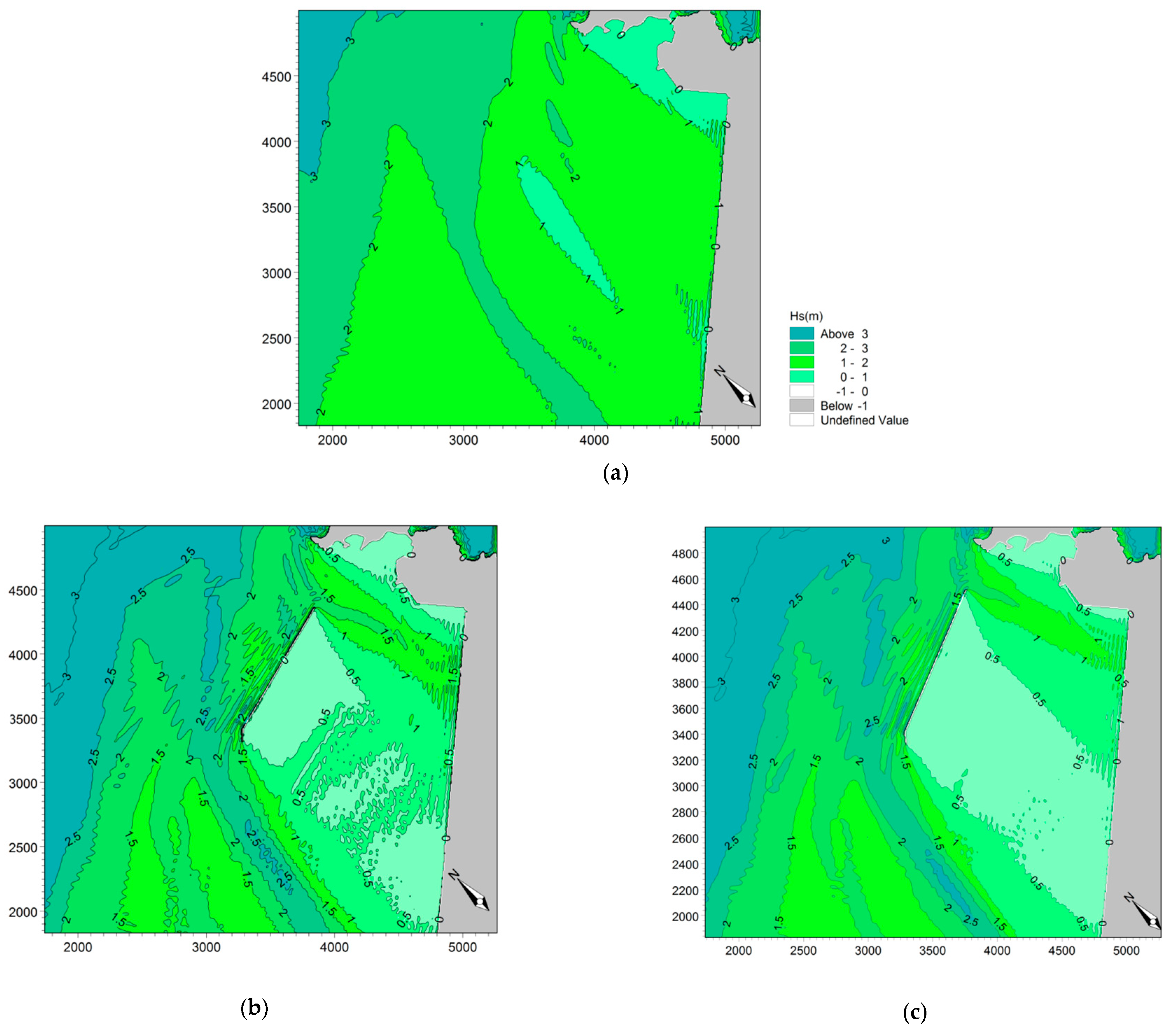
Figure 12.
Distribution of significant wave height in the NNE direction under three working conditions: (a) before the project, (b) Scheme 1, (c) Scheme 2. Notes: In the figure, wave height vaules and plane coordinates are all in meters.
Figure 12.
Distribution of significant wave height in the NNE direction under three working conditions: (a) before the project, (b) Scheme 1, (c) Scheme 2. Notes: In the figure, wave height vaules and plane coordinates are all in meters.
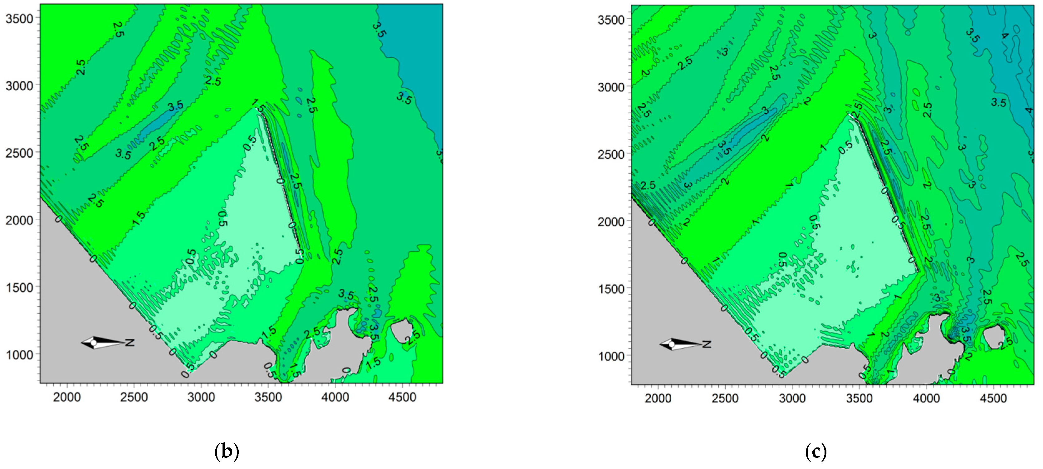
Figure 13.
Distribution of significant wave height in the NE direction under three working conditions: (a) before the project, (b) Scheme 1, (c) Scheme 2. Notes: In the figure, wave height vaules and plane coordinates are all in meters.
Figure 13.
Distribution of significant wave height in the NE direction under three working conditions: (a) before the project, (b) Scheme 1, (c) Scheme 2. Notes: In the figure, wave height vaules and plane coordinates are all in meters.
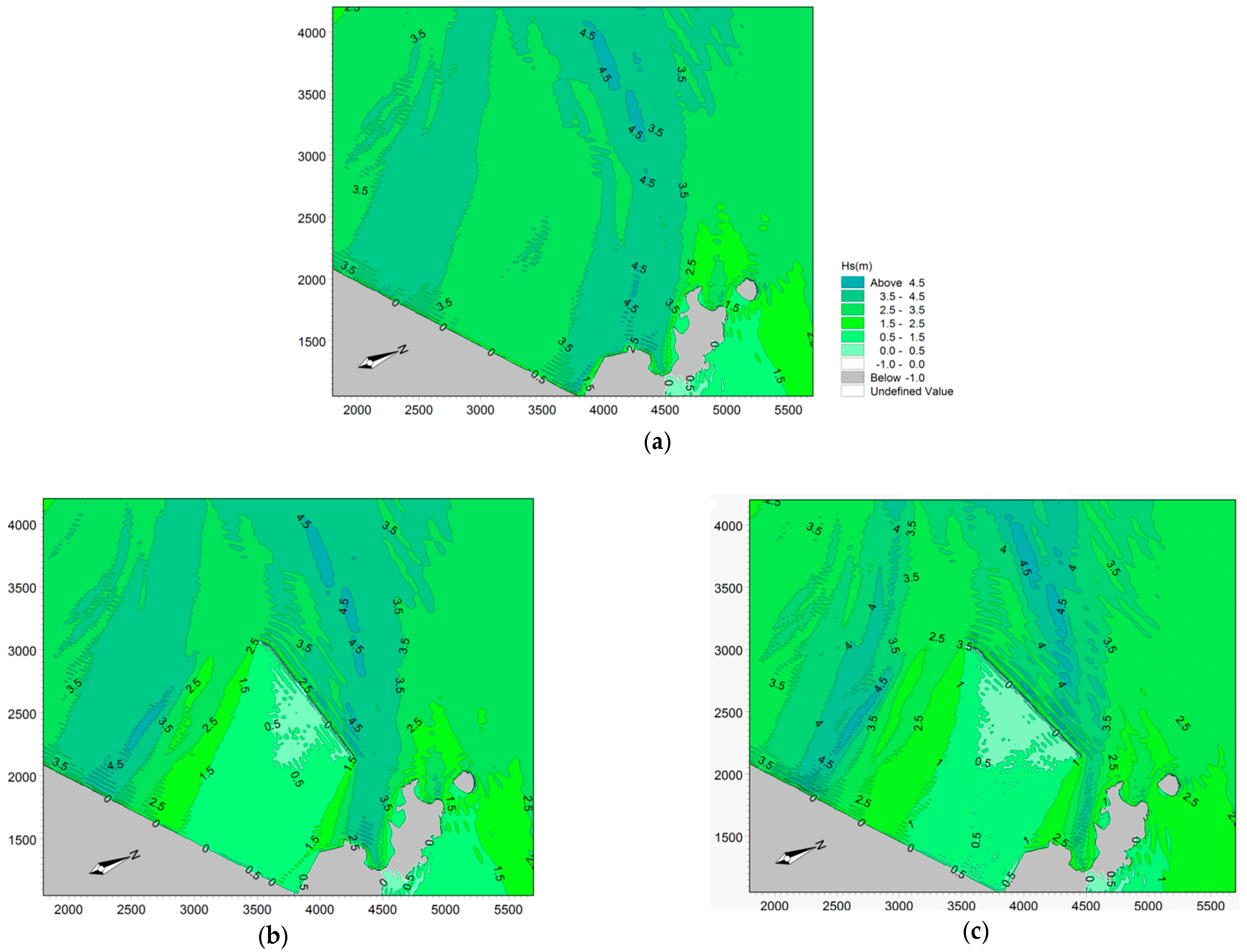
Figure 14.
Distribution of significant wave height in the W direction under three working conditions: (a) before the project, (b) Scheme 1, (c) Scheme 2. Notes: In the figure, wave height vaules and plane coordinates are all in meters.
Figure 14.
Distribution of significant wave height in the W direction under three working conditions: (a) before the project, (b) Scheme 1, (c) Scheme 2. Notes: In the figure, wave height vaules and plane coordinates are all in meters.
Figure 15.
Distribution of significant wave height in the WNW direction under three working conditions: (a) before the project, (b) Scheme 1, (c) Scheme 2. Notes: In the figure, wave height vaules and plane coordinates are all in meters.
Figure 15.
Distribution of significant wave height in the WNW direction under three working conditions: (a) before the project, (b) Scheme 1, (c) Scheme 2. Notes: In the figure, wave height vaules and plane coordinates are all in meters.
Figure 16.
Distribution of significant wave height in the NW direction under three working conditions: (a) before the project, (b) Scheme 1, (c) Scheme 2. Notes: In the figure, wave height vaules and plane coordinates are all in meters.
Figure 16.
Distribution of significant wave height in the NW direction under three working conditions: (a) before the project, (b) Scheme 1, (c) Scheme 2. Notes: In the figure, wave height vaules and plane coordinates are all in meters.
Figure 17.
Wave feature points of the breakwater.
Figure 17.
Wave feature points of the breakwater.
Figure 18.
Wave feature points of the pier.
Figure 18.
Wave feature points of the pier.
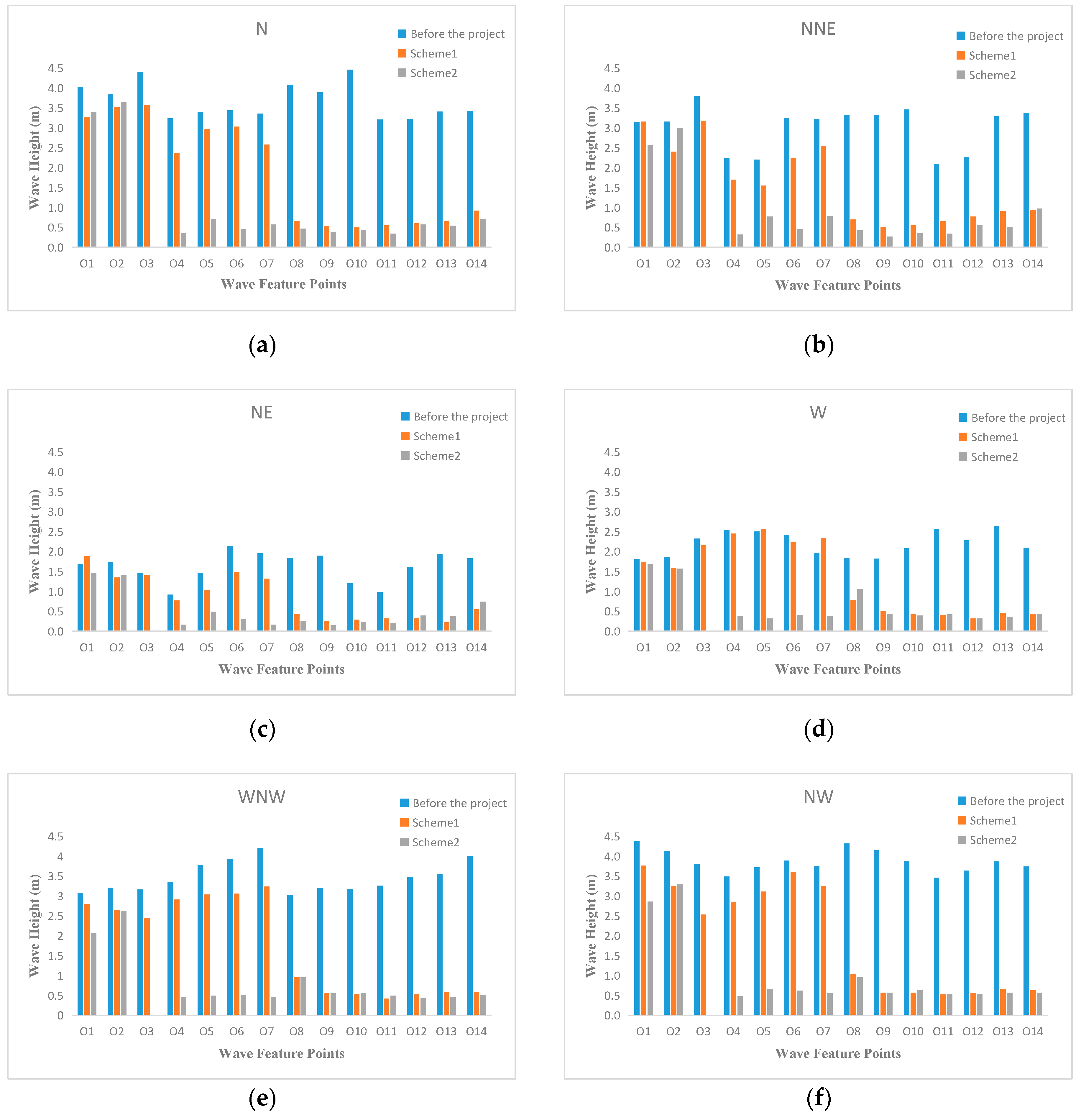
Figure 19.
Wave parameters at the feature points of different schemes. (a) wave height vaules of wave coming from N direction at O1–O14 under three working conditions, (b) wave height vaules of wave coming from NNE direction, (c) wave height vaules of wave coming from NE direction, (d) wave height vaules of wave coming from W direction, (e) wave height vaules of wave coming from WNW direction, (f) wave height vaules of wave coming from NW direction.
Table 1.
Wind speeds at the Jinjimen weather station in different return periods (unit: m/s).
Table 1.
Wind speeds at the Jinjimen weather station in different return periods (unit: m/s).
| Wind Direction | Once in 50 Years | Once in 2 Years |
|---|
| WSW | 28.3 | 13.9 |
| W | 27.4 | 13.2 |
| WNW | 29.7 | 20.4 |
| NW | 26.2 | 20.1 |
| NNW | 35.7 | 23.5 |
Table 2.
Calibration values of wave parameters in different return periods.
Table 2.
Calibration values of wave parameters in different return periods.
| Wave Direction | Hs (m)1 | Ts (s)2 |
|---|
| Once in 50 Years | Once in 2 Years | Once in 50 Years | Once in 2 years |
|---|
| WSW | 3.63 | 2.04 | 7.69 | 5.76 |
| W | 3.59 | 1.99 | 7.65 | 5.70 |
| WNW | 3.86 | 2.93 | 7.93 | 6.91 |
| NW | 3.69 | 2.98 | 7.75 | 6.97 |
| NNW | 4.23 | 3.09 | 8.30 | 7.09 |
Table 3.
Calibration values of wave parameters during different return periods.
Table 3.
Calibration values of wave parameters during different return periods.
| Wave Direction | Hs (m) | Ts (s) |
|---|
| Once in 50 Years | Once in 2 Years | Once in 50 Years | Once in 2 Years |
|---|
| N | 4.55 | 2.92 | 8.58 | 6.88 |
| NNE | 8.01 | 2.95 | 11.38 | 6.90 |
| NE | 10.76 | 2.90 | 13.20 | 6.85 |
| ENE | 4.98 | 3.00 | 8.98 | 6.97 |
| E | 8.74 | 2.99 | 11.82 | 6.82 |
| ESE | 9.93 | 2.69 | 12.67 | 6.59 |
Table 4.
Layout of the breakwater.
Table 4.
Layout of the breakwater.
| Calculation Scheme | Layout of Breakwater |
|---|
| Scheme 1 | The total length of the breakwater is 1200 m: the broken line section on the west side is 100 m long, and that on the east is 1100 m long. |
| Scheme 2 | The total length of the breakwater is 1300 m: the broken line section on the west side is 100 m long, and that on the east is 1200 m long. In addition, Scheme 2 was rotated 8 degrees counterclockwise along the axis on the basis of Scheme 1. |
Table 5.
Plane coordinates of the wave feature points (unit: m).
Table 5.
Plane coordinates of the wave feature points (unit: m).
| Location of Feature Points | Feature Points | x-Coordinate | y-Coordinate | Feature Points | x-Coordinate | y-Coordinate |
|---|
| Both sides of the breakwater | O1 | 418,535.9 | 3,358,763.6 | O8 | 418,603.9 | 3,358,714.0 |
| O2 | 418,601.6 | 3,358,828.1 | O9 | 418,625.8 | 3,358,768.2 |
| O3 | 418,819.5 | 3,358,883.5 | O10 | 418,836.8 | 3,358,818.9 |
| O4 | 419,031.6 | 3,358,938.8 | O11 | 419,048.9 | 3,358,875.4 |
| O5 | 419,244.9 | 3,358,990.7 | O12 | 419,261.0 | 3,358,930.7 |
| O6 | 419,458.2 | 3,359,044.9 | O13 | 419,474.3 | 3,358,984.9 |
| O7 | 419,647.2 | 3,359,093.3 | O14 | 419,661.1 | 3,359,033.3 |
| Pier front | W1 | 419,103.9 | 3,358,447.1 | W4 | 419,343.5 | 3,358,511.0 |
| W2 | 419,178.0 | 3,358,468.9 | W5 | 419,411.7 | 3,358,528.4 |
| W3 | 419,262.2 | 3,358,490.7 | | | |
Table 6.
Area table.
| Schemes | Statistical Indexes | N | NNE | NE | W | WNW | NW |
|---|
| Scheme 1 | Covering area (km2) | 0.37 | 0.52 | 1.31 | 1.03 | 0.43 | 0.19 |
| Scheme 2 | Covering area (km2) | 0.69 | 0.80 | 2.06 | 1.32 | 0.88 | 0.30 |
| Rate of change (%) | 88.51 | 53.90 | 56.78 | 28.30 | 103.36 | 55.97 |
Table 7.
Berthing stability analysis of Scheme 1 (unit: m). Y stands for safe berthing of ships and N means unsafe berthing.
Table 7.
Berthing stability analysis of Scheme 1 (unit: m). Y stands for safe berthing of ships and N means unsafe berthing.
| | W1 | | W2 | | W3 | | W4 | | W5 | |
|---|
| N | 0.5 | Y | 0.56 | Y | 0.57 | Y | 0.51 | Y | 0.5 | Y |
| NNE | 0.45 | Y | 0.44 | Y | 0.46 | Y | 0.43 | Y | 0.45 | Y |
| NE | 0.34 | Y | 0.32 | Y | 0.29 | Y | 0.29 | Y | 0.27 | Y |
| W | 0.52 | Y | 0.45 | Y | 0.34 | Y | 0.29 | Y | 0.26 | Y |
| WNW | 0.84 | N | 0.66 | N | 0.51 | Y | 0.52 | Y | 0.43 | Y |
| NW | 0.89 | N | 0.76 | N | 0.59 | Y | 0.58 | Y | 0.56 | Y |
Table 8.
Berthing stability analysis of Scheme 2 (unit: m). Y stands for safe berthing of ships and N means unsafe berthing.
Table 8.
Berthing stability analysis of Scheme 2 (unit: m). Y stands for safe berthing of ships and N means unsafe berthing.
| | W1 | | W2 | | W3 | | W4 | | W5 | |
|---|
| N | 0.34 | Y | 0.33 | Y | 0.32 | Y | 0.35 | Y | 0.41 | Y |
| NNE | 0.27 | Y | 0.28 | Y | 0.35 | Y | 0.37 | Y | 0.39 | Y |
| NE | 0.24 | Y | 0.25 | Y | 0.28 | Y | 0.25 | Y | 0.24 | Y |
| W | 0.58 | Y | 0.53 | Y | 0.39 | Y | 0.33 | Y | 0.28 | Y |
| WNW | 0.59 | Y | 0.56 | Y | 0.5 | Y | 0.46 | Y | 0.43 | Y |
| NW | 0.58 | Y | 0.57 | Y | 0.53 | Y | 0.55 | Y | 0.51 | Y |


