Analysing the Relationship between Multiple-Timescale SPI and GRACE Terrestrial Water Storage in the Framework of Drought Monitoring


Joint Research Centre (JRC), European Commission, 21027 Ispra, Italy
*
Author to whom correspondence should be addressed.
Water 2019, 11(8), 1672; https://doi.org/10.3390/w11081672
Submission received: 12 July 2019
/
Revised: 9 August 2019
/
Accepted: 10 August 2019
/
Published: 13 August 2019
(This article belongs to the Special Issue Droughts and Floods Assessment and Monitoring Using Remote Sensing and Geospatial Techniques)
Abstract
:The operational monitoring of long-term hydrological droughts is often based on the standardised precipitation index (SPI) for long accumulation periods (i.e., 12 months or longer) as a proxy indicator. This is mainly due to the current lack of near-real-time observations of relevant hydrological quantities, such as groundwater levels or total water storage (TWS). In this study, the correlation between multiple-timescale SPIs (between 1 and 48 months) and GRACE-derived TWS is investigated, with the goals of: (i) evaluating the benefit of including TWS data in a drought monitoring system, and (ii) testing the potential use of SPI as a robust proxy for TWS in the absence of near-real-time measurements of the latter. The main outcomes of this study highlight the good correlation between TWS anomalies (TWSA) and long-term SPI (12, 24 and 48 months), with SPI-12 representing a global-average optimal solution (R = 0.350 ± 0.250). Unfortunately, the spatial variability of the local-optimal SPI underlines the difficulty in reliably capturing the dynamics of TWSA using a single meteorological drought index, at least at the global scale. On the contrary, over a limited area, such as Europe, the SPI-12 is able to capture most of the key traits of TWSA that are relevant for drought studies, including the occurrence of dry extreme values. In the absence of actual TWS observations, the SPI-12 seems to represent a good proxy of long-term hydrological drought over Europe, whereas the wide range of meteorological conditions and complex hydrological processes involved in the transformation of precipitation into TWS seems to limit the possibility of extending this result to the global scale.
1. Introduction
The last few decades have seen an increasing awareness of the worldwide socioeconomic repercussions of droughts [1], with annual average economic losses quantified at $6–8 billion for the United States [2], and about €3–6 billion for the European Union [3]. Numerous studies have highlighted the prominent role of drought among natural hazards (e.g., Bryant [4]) and much effort has been put into promoting a transition in the paradigm adopted to face drought from a reactive to a proactive approach (e.g., References [5,6,7]). Within this context, the development of an effective drought early warning and monitoring system (DEWS) represents one of the key pillars for a successful integrated drought management system [5].
Over Europe, the Joint Research Centre (JRC) of the European Commission has established the European Drought Observatory (EDO, http://edo.jrc.ec.europa.eu), which aims at capturing the spatio-temporal evolution of droughts, with special regard paid to trans-boundary events. Given the creeping nature of drought phenomena, as well as the large array of socio-economic and environment sectors that can be affected by droughts, a variety of indicators have been adopted in EDO to fully characterise the main traits of drought events in order to provide insightful advice to stakeholders and policy makers. Currently, both meteorological and agricultural drought conditions are continuously updated in EDO through various indicators, ranging from the standardised precipitation index (SPI) computed over multiple aggregation periods to modelled soil moisture and remotely sensed vegetation anomalies [8]. Additionally, short-term hydrological droughts are also monitored after the introduction of a river discharge low-flow index [9].
More recently, a parallel global-scale monitoring system has been implemented, namely the Global Drought Observatory (GDO, http://edo.jrc.ec.europa.eu/gdo/), with a greater focus on supporting the Emergency Response Coordination Centre (ERCC) of the European Commission. Although additional indicators specifically focusing on dynamic drought risk assessment are implemented in GDO, the base indicators used to monitor the propagation of drought hazard within the hydrological cycle are analogous to those available in EDO.
In spite of its key role in both water supply and irrigation, long-term hydrological drought (also referred to as groundwater drought) is often under-represented in operational large-scale monitoring systems, such as EDO and GDO. This is mainly due to the lack of near-real-time data [10], as well as the challenges in an effective groundwater schematisation in hydrological and land surface models [11]. The relevance of monitoring groundwater and other slow-responding variables as complementary information to other more faster-responding hydrological variables, such as soil moisture or river discharge, is highlighted by the numerous studies analysing past droughts using historical datasets (i.e., References [12,13,14]).
In March 2002, the Gravity Recovery and Climate Experiment (GRACE) mission was launched [15] with the aim of providing satellite observations of the terrestrial gravity field. Within the framework of hydrological applications, this dataset represented an unprecedented stream of data to globally monitor the dynamics of the total terrestrial water storage (TWS; the sum of all above and below surface water storages, including canopy water, rivers and lakes, soil moisture and groundwater) [16]. Following the decommissioning of the GRACE satellites in October 2017, a follow-on mission, namely the GRACE-FO, was successfully launched in May 2018 in order to ensure continuity in the Earth’s gravity measurements collected by its predecessor.
The potential of GRACE for drought monitoring has been investigated in the past, especially focusing on the assimilation of TWS data in land surface models [17,18,19]. Outcomes of those studies have highlighted the capability of GRACE products to improve the skill of land surface models in reproducing groundwater dynamics [20], but also the limited capability of the global models to capture the amplitude of the GRACE TWS time series [21,22]. With the increasing length of GRACE data records, a growing number of studies have also evaluated the capability of GRACE TWS to directly infer the severity and timing of long-term droughts, often focusing on specific regions [23,24,25,26,27] or drought events [28,29,30,31,32]. Due to its monthly aggregation and coarse spatial resolution (i.e., one degree), the direct use of GRACE products for near-real-time applications at finer spatial scales (i.e., water basins) has been questioned (see References [17,30,33]). On the one hand, Van Loon et al. [30] highlighted how GRACE products were not able to capture the locally-observed spatial dynamics of the 2015 European groundwater drought, likely due to the coarse spatial resolution, even if some temporal traits of both 2003 and 2015 events were correctly identified. On the other hand, Long et al. [29] demonstrated a good capability of GRACE to quantify the total water storage depletion during the extreme drought event in 2011 in Texas.
On the contrary, analyses at the global scale are limited, with Humphrey et al. [34] performing an analysis of the different components of the GRACE-derived TWS signal, highlighting the major role of the long-term variability and the relationship with dominant atmospheric drivers (i.e., precipitation and temperature). In Sun et al. [35], a breakpoint detection method has been applied to GRACE products in order to derive extreme events over 35 major river basins all over the globe, investigating the relationship between TWS anomalies and the 3-month SPI.
Both local and global studies have highlighted the strong connection between TWS anomalies and rainfall data, suggesting that more classical meteorological drought indices (i.e., SPI) accumulated over long periods can be used as proxies of long-term hydrological drought in the absence of groundwater measurements [36,37]. This approach is supported by the assumption that groundwater responds to precipitation over long temporal scales. However, even if some studies have found a good correlation between regional-average groundwater time series and long-term precipitation [38], the optimal accumulation period for precipitation seems to vary considerably in space, depending on the area of interest (see References [30,39,40]).
Nevertheless, the relationship between SPI at different temporal aggregation scales and GRACE TWS anomalies can be exploited to better understand the propagation of drought through the hydrological cycle, as schematised in Changnon Jr. [41], as well as to identify possible spatially coherent patterns in such a relationship. Within the framework of the potential use of upcoming GRACE-FO data for drought monitoring, understanding the connection between the basic meteorological drought indices and the already available GRACE products can be helpful for future evaluations of the reliability of the new dataset and its consistency with the time series provided by its predecessor.
Following these considerations, the main goal of this study was to analyse the relationship between the SPI dataset currently used in the operational monitoring of meteorological drought in EDO and GDO and the monthly standardised anomalies derived from the GRACE TWS, with the former aggregated at different timescales ranging from 1 to 48 months, and by considering different time lags (up to 3 months). The focus of this analysis was twofold: (i) to understand the actual value of GRACE products as a tool for long-term drought monitoring under the hypothesis that TWS is a good proxy of groundwater storage, and its potential role in both continental and global scale drought monitoring systems, where the coarse spatial detail of TWS data is not a strong limitation; and (ii) to investigate the spatial consistency of the SPI–TWS relationship, with the aim to evaluate the use of SPI as a proxy for TWS in the absence of GRACE-derived or other TWS datasets.
In view of the forthcoming release of GRACE-FO TWS products, the outcomes of these analyses can also be used as a benchmark for evaluating the future integration of GRACE-FO into the EDO and GDO monitoring systems.
2. Materials and Methods
2.1. GRACE Terrestrial Water Storage Anomalies
The Gravity Recovery and Climate Experiment (GRACE) mission was launched in March 2002 with the goal to measure variations in the terrestrial gravity field [15]. The GRACE mission consisted of a pair of identical satellites, both orbiting at an altitude of about 450–500 km and around 200 km apart. Precise variations in the distance between the two satellites were measured by means of a microwave ranging system, and successively converted into temporal variations in Earth’s gravity field.
For land hydrological applications, the terrestrial water storage (TWS) change is derived from the surface mass change after removing the atmospheric and oceanic contributions, which are better constrained and easier to reconstruct [42]. This land product is derived from a gravity field composed of a set of spherical harmonic coefficients (up to a maximum order/degree of 60) after a series of post-processing procedures (see Landerer and Swenson [43] for details), which include smoothing [44], destriping [45] and glacial isostatic adjustment [46]. In addition, grid-based scaling is introduced in order to restore the signal amplitude lost due to the application of smoothing and destriping filters [47], and TWS data are finally reported not as absolute values, but as deviations from the long-term 2004–2009 mean value.
This study used the TWS product (version RL05) produced by the Center for Space Research (CSR) at the University of Texas at Austin, as scaled by the NASA Jet Propulsion Laboratory (JPL) (available at: https://grace.jpl.nasa.gov/data/get-data/monthly-mass-grids-land/). These data are aggregated monthly at a 1° spatial resolution and available from April 2002 to January 2017. It should be noted that since early 2011, the GRACE instruments were periodically turned off due to active battery management, causing some missing monthly data. Additionally, even if the nominal spatial resolution of the product is 1°, neighbouring cells are not completely independent since spatial smoothing is applied.
In order to analyse the role of GRACE products in drought applications, monthly TWS anomalies (TWSA) were derived from the original dataset, using the period 2002–2016 for the computation of the baseline climatology monthly statistics, as:
where the subscripts i and j represent the month (from 1 to 12) and the year, respectively, and the baseline average (μi) and standard deviation (σi) for a given month are computed only if at least 10 years of monthly data were available in the baseline.
2.2. GDO Multiple-Timescale SPI
The standardized precipitation index (SPI), first introduced by McKee et al. [48], is the most commonly used meteorological drought indicator, thanks to its flexibility and ease of use [49]. The SPI standardises the deviation of precipitation at different accumulation periods (commonly between 1 and 48 months) at a particular location with the long-term climatological conditions for the same period. Even if SPI is generally used to monitor the occurrence of meteorological droughts, medium- (e.g., 3–6 months) and long- (e.g., 12–24 months) term accumulation periods are often used as proxies for agricultural and hydrological droughts.
Following the guidelines reported by the World Meteorological Organization [49] to regulate the SPI computation, the period 1981–2010 is used in the GDO as the baseline for the fitting of a gamma distribution on the non-zero rainfall data, according to the maximum likelihood method [50]. GDO SPI maps at 1° are derived from monthly precipitation data provided by the Global Precipitation Climatology Centre (GPCC—http://gpcc.dwd.de/). Specifically, a “first guess” product is used for the two months prior to the current month, whereas the consolidated “monitoring” product is used for the antecedent months.
Several SPI accumulation periods are available from EDO and GDO, with SPI-1, 3, 6, 9, 12, 24 and 48 months used in this study, including only the “monitoring” dataset available between 2002 and 2016, which is the period overlapping with the GRACE dataset. Due to the well-known underestimation of dry SPI values over areas and periods characterised by frequent zero rainfall months [51], the areas with average year-total rainfall lower than 100 mm were masked, which mostly include the Sahara, Arabian and Gobi deserts. Additionally, due to the lack of rainfall measurements and liquid precipitation, Greenland was masked out from the analysis.
2.3. Evaluation Strategy
Even if SPI has been used as a proxy for hydrological droughts, the actual relationship between SPI and TWSA is likely related to various local factors that control the response of aquifers to precipitation, including catchments and geological characteristics [52]. Correlation between SPI at different temporal aggregation and TWSA is evaluated through the Pearson correlation coefficient, R, which allows the identification of the SPI-n (n = 1, 3, 6, 9, 12, 24, 48) with the highest R value for each 1° cell. Given the standardised nature of both SPI and TWSA, R can be considered a good metric of the agreement between the datasets. In addition, a temporal delay can be expected in the response of TWS to rainfall deficits, especially for short aggregation periods; for this reason, a lagged correlation analysis was also performed between SPI-n and TWSA with delays of up to 3 months.
According to the global-average R value for each SPI-n versus TWSA pair, a global-optimal SPI can be identified as the SPI that best explains on average the variations in TWSA (i.e., highest global-average R). The difference between local-optimal SPI and global-optimal SPI can be computed at each cell, and the statistical significance of this difference can be evaluated according to Steiger [53], based on the Fisher z-transformation of the R values. This test allows to identify the cells where the global-optimal SPI is not a suitable substitute of the local-optimal one.
In addition to random errors, quantified using R, standardised quantities may display systematic discrepancies if different baseline periods are used, as in the case of SPI (1981–2010) and TWSA (2002–2016). Those biases can be quantified by means of a linear transformation procedure that matches the long-term average and standard deviation of SPI-n in the period 2002–2016 to the ones of TWSA for the same period (which, by definition, are equal to 0 and 1, respectively, due to the standardisation) [54]. Those systematic differences are removed from the analysis since they are unrelated to the stochastic nature of droughts, but only due to the difference in the adopted baselines.
While correlation analysis gives an overall estimation of the agreement between two standardised datasets, a special focus on extreme values can be relevant for drought studies. In this case, we subdivided both SPI and TWSA values into seven classes, following McKee et al. [48]: a near-normal class (−1 < SPI < 1), three drier than normal (−1.5 < SPI ≤ −1, −2 < SPI ≤ −1.5 and SPI ≤ −2) and three wetter than normal (1 ≤ SPI < 1.5, 1.5 ≤ SPI < 2 and SPI ≥ 2) classes. This categorisation allows for a direct comparison of the frequency distribution of the values in these seven classes for the two datasets.
3. Results and Discussion
The global-scale correlation between both TWS and TWSA against multiple-timescale SPIs was first investigated, with the aim to detect relevant spatial patterns and optimal sets of SPI. This analysis is followed by an in-depth analysis of the results over Europe, with the goal being to test the possibility of adopting a single SPI dataset as a proxy of TWSA over the region.
3.1. Global Correlation Analysis
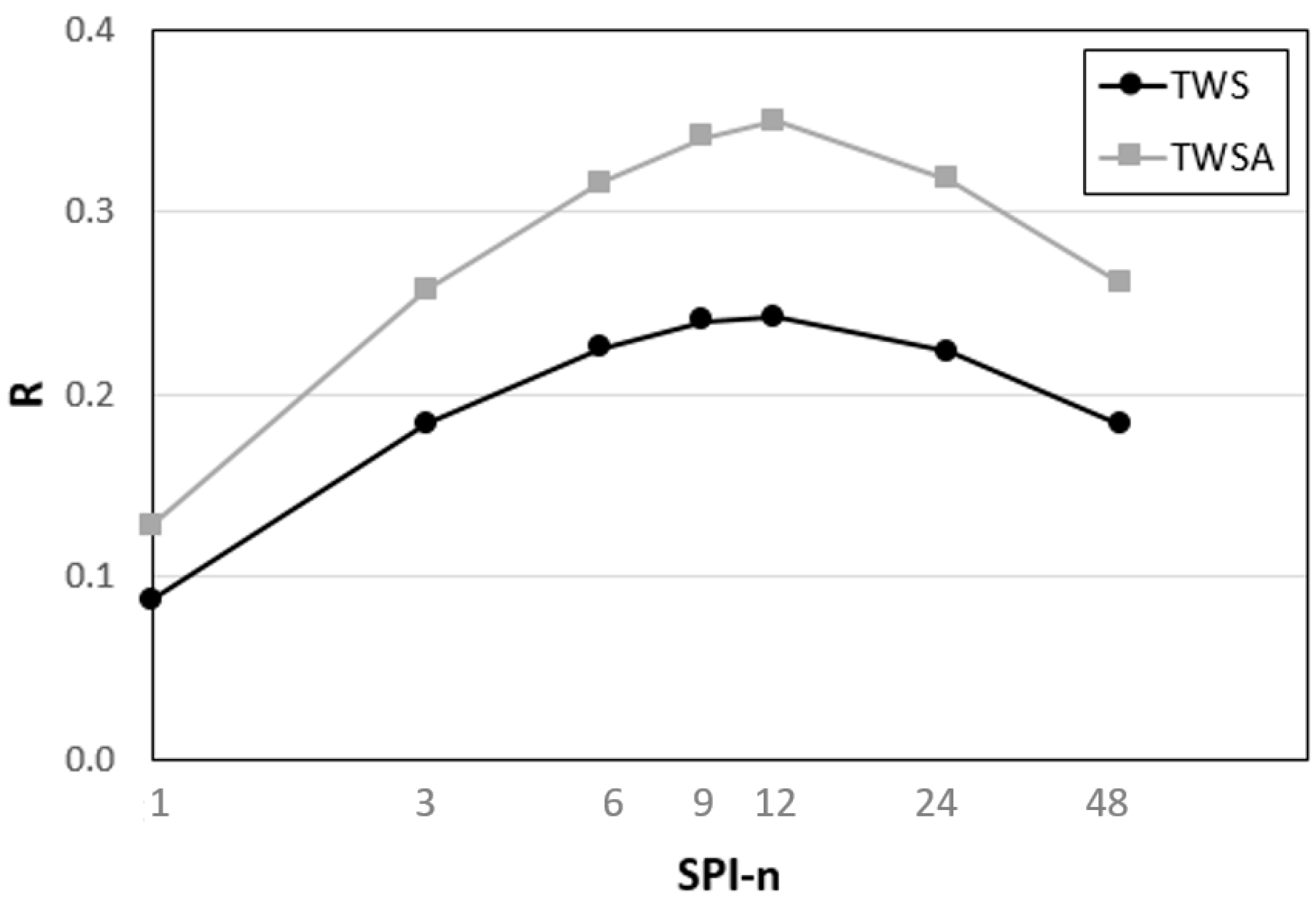
A total of 14 correlation analyses were performed by pairing the seven SPIs at different accumulation periods with both TWS and TWSA. The global-average R values are reported in the plot in Figure 1 as a synthetic descriptor of the overall relationship between the set of SPI datasets and the two GRACE-derived indices.
The results reported in Figure 1 show how the global-average correlation between SPI and TWSA was always higher (on average) compared to TWS, with a larger improvement for the highest average R values. Overall, the global-average R values for both TWS and TWSA displayed a similar behaviour, with a concave shape and a peak at SPI-12. While SPI-12 and SPI-9 performed relatively close to each other, the improvement over SPI-48, SPI-1 and SPI-3 was rather clear.
Given the definition of TWS, which includes slowly-responding hydrological variables, such as groundwater, the good correlation with longer accumulation period indices (i.e., SPI-12) was expected, confirming the anticipated possibility of using a GRACE-derived TWSA as a proxy for long-term hydrological droughts. Additionally, the improved results obtained by contrasting SPI with TWSA, compared to TWS, confirm the need for standardising the TWS data (see Equation (1)) in order to obtain an indicator that is comparable with SPIs. Based on this latter consideration, the successive analyses are focused on the TWSA dataset only, as the better proxy of droughts compared to the simple TWS.
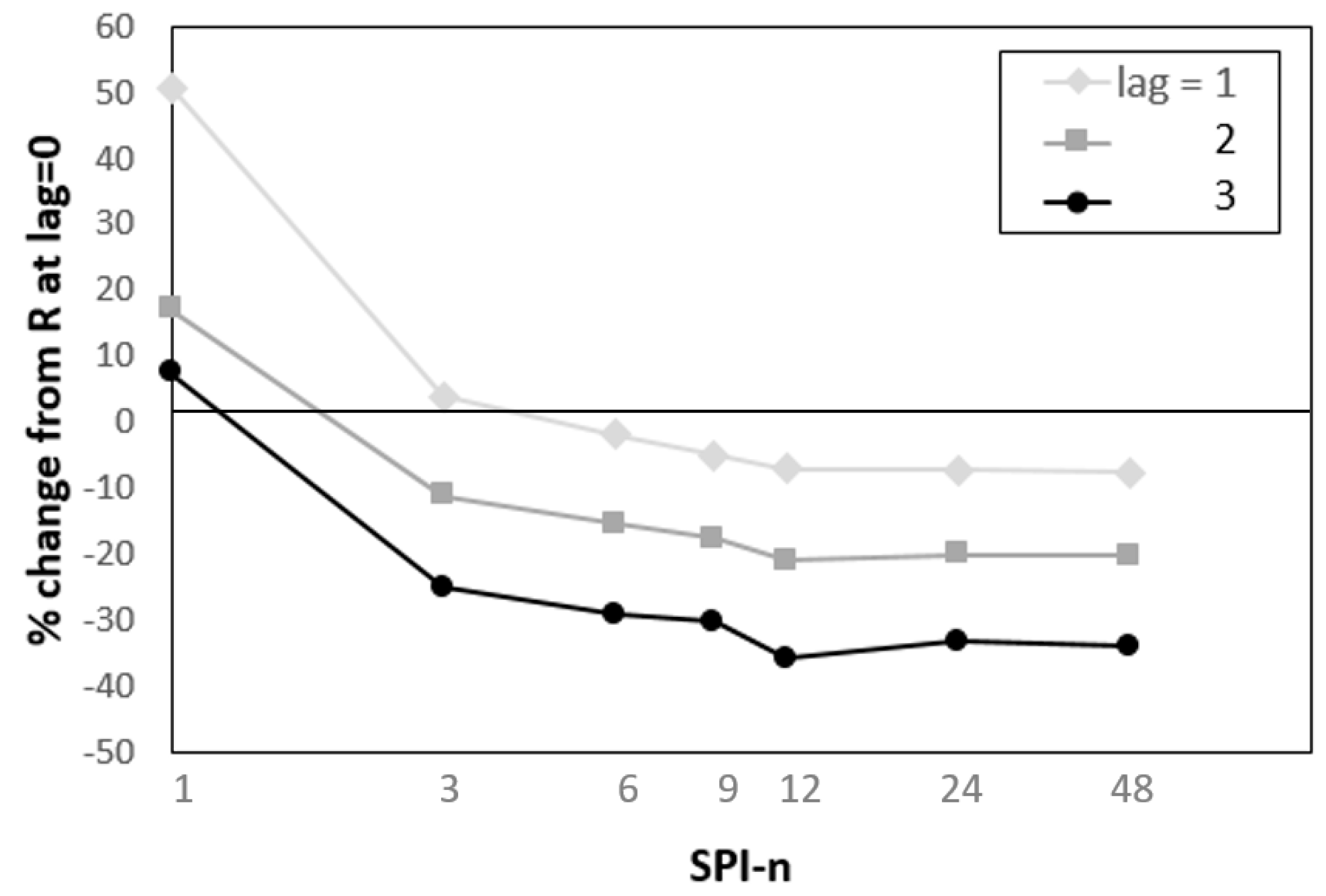
Following the analogy between TWSA and long-term hydrological drought, a temporal delay may be expected in the response of TWSA to SPIs. For this reason, a temporal lag of up to 3 months was introduced into the correlation analysis, highlighting how a slight improvement can be obtained for short-accumulation periods (SPI-1 and partially SPI-3, see Figure 2), whereas no improvements were achieved for longer accumulation periods. The results depicted in Figure 2 show how the increase in R was more marked for SPI-1 than for SPI-3, with an increase in correlation for both indices in the case of a one-month time lag. However, in both cases, the maximum R value never reached the ones obtained for SPI-9 and SPI-12 without a time lag (Figure 1). This behaviour can be explained by the time needed for slow-responding variables (i.e., groundwater) to react to the short-term variations in precipitation captured by SPI-1 and SPI-3, whereas the long-term SPIs already intrinsically account for this delay through accumulating the rainfall over a long antecedent time window.
Even if SPI-12 had the highest global-average R value (0.350 ± 0.250), different optimal accumulation periods can be defined locally for each cell in order to optimize the overall average R. The map in Figure 3 shows the spatial distribution of the maximum R value for each cell, without accounting for lag, obviously returning an overall global-average R higher than the one for SPI-12 (0.445 ± 0.224). In addition, the map in Figure 4 depicts the spatial distribution of the local-optimal SPI accumulation period, corresponding to the maximum R represented in Figure 3.
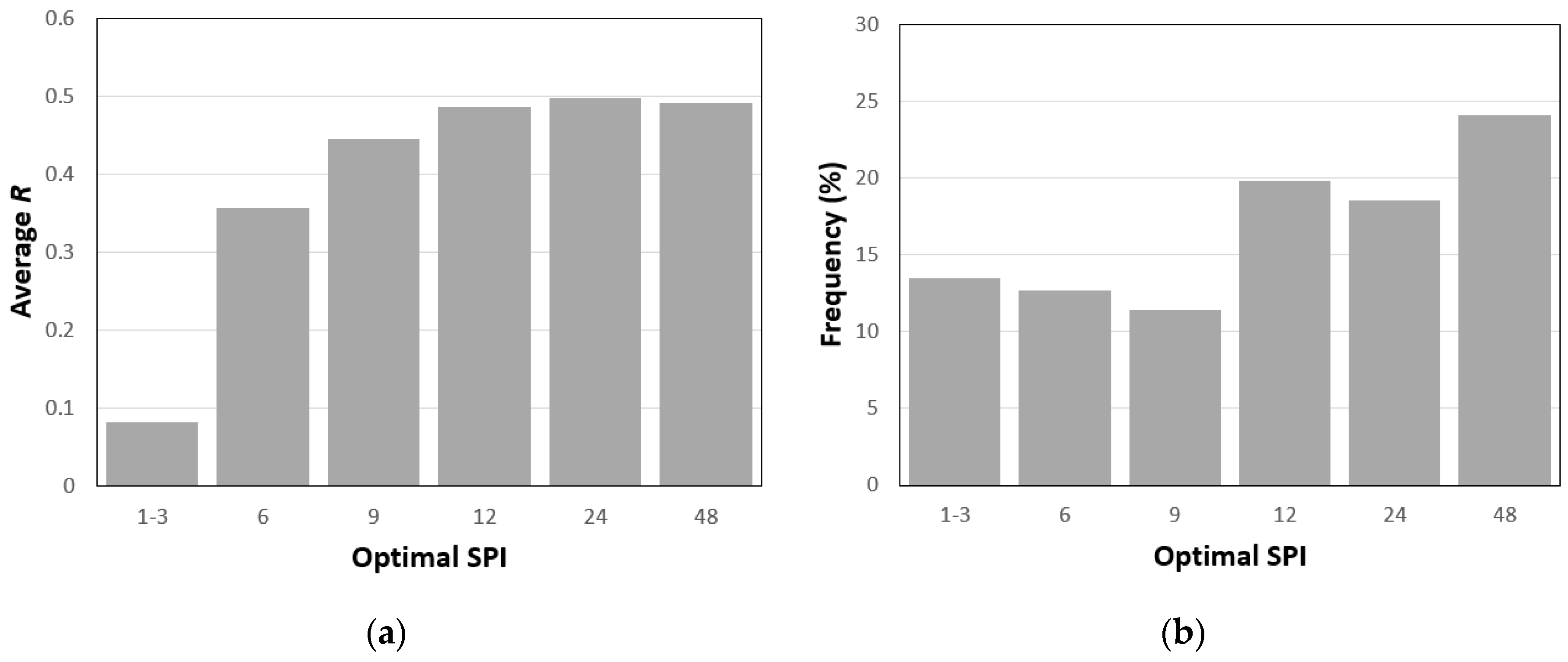
The map in Figure 3 highlights how even the maximum R value among the seven values derived from the SPI-TWSA correlation analyses were not significant (or even negative) over some areas (red and light-yellow cells, about 10% of the spatial domain), including most notably over eastern Canada, western and central Africa, Afghanistan and part of south-east Asia. This suggests that none of the SPI datasets available in GDO appeared to capture the TWSA dynamics over these specific regions. The majority of the areas with a maximum R < 0.12 had the highest correlation for short-term SPIs (1 or 3, see Figure 4), a result that is further corroborated by the average R values for each optimal SPI class, as reported in Figure 5a. The cells where SPI-1/SPI-3 were the optimal were those with a very low average R, whereas the average R for all the other SPIs was quite similar, suggesting that an optimal correlation between 0.4 and 0.5 could be achieved on average if the correct SPI was used.
The map in Figure 4 shows that even if SPI-12 had the highest global-average R value (see Figure 1), this solution was not the optimal one over the majority of the cells, being the outcome only for about 20% of the cases, as shown in Figure 5b. Overall, SPI-48 had the highest share of cells where it represented the optimal solution (close to 25%), but it was clear that none of the indices from SPI-12 to 48 were able to clearly outperform the others consistently.
Overall, a visual comparison between the spatial distribution of the optimal SPI depicted in Figure 4 and commonly available global datasets of groundwater characteristics, such as the maps provided by the World-wide Hydrological Mapping and Assessment Programme (WHYMAP, https://www.whymap.org/), did not suggest any clear relationship. Given the complex nature of TWS, which summarises numerous hydrological quantities and complex interactions, it is not surprising that a combination of several factors may be needed to explain its spatio-temporal dynamics. However, since about 2/3 of the globe has an optimal correlation with SPI-12 to SPI-48, it seems possible to generally conclude that TWSA successfully summarises those long-term droughts that are often underrepresented in global monitoring tools.
3.2. Use of a Single SPI as a Proxy for TWSA
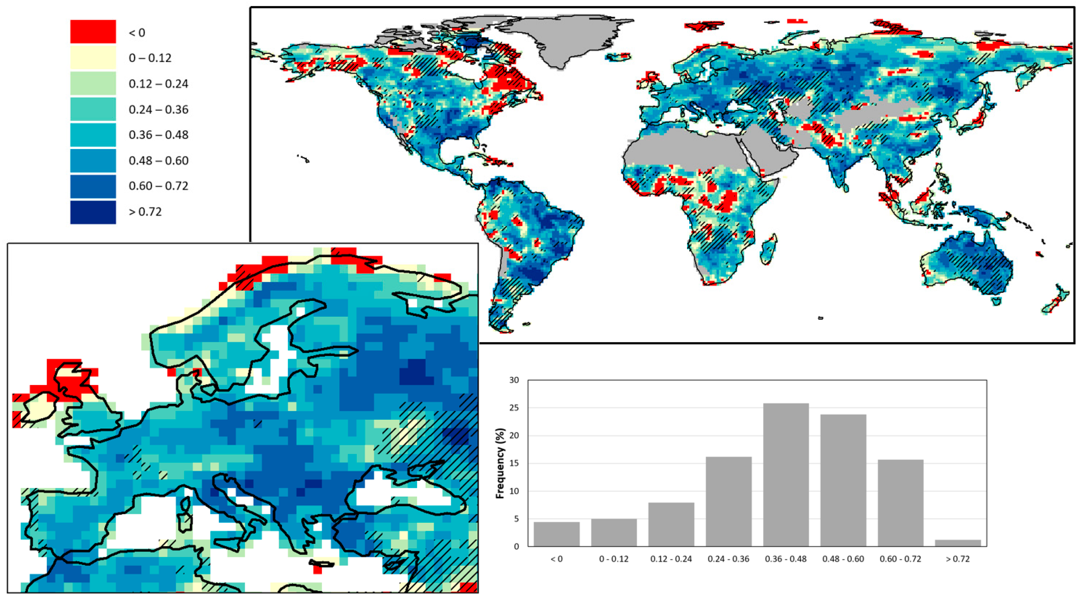
On the one hand, the results depicted in Figure 3 and Figure 4 highlight the large spatial variability in the optimal SPI dataset that best describes the dynamics of GRACE-derived TWSA (i.e., local-optimal). On the other hand, according to the global-average results synthesised in Figure 1, SPI-12 seems the overall best option (i.e., global-optimal) to capture TWSA if only a single indicator can be used. To investigate the extent to which SPI-12 can be used as a proxy of TWSA globally, the map in Figure 6 (main panel) represents the spatial distribution of R values between SPI-12 and TWSA, with the strip-filling highlighting the cells where there was a statistically significant (p ≤ 0.05) difference between this value and the local-optimal one depicted in Figure 3.
Compared to Figure 3, the map in Figure 6 shows both an increase in the frequency of cells with R < 0.12 (red and light-yellow), as well as some clear spatial patterns of the stripped cells, such as over the Middle East, Australia, southern-central Africa and southern Latin America. Overall, about 20% of the domain had a statistically significant difference between the local and the global optimal R values, even if it was possible to detect large areas with a minimal impact. In particular, over Europe, most of the region showed no significant difference (see Figure 6, lower-left corner), with the only notable exception over Ukraine. On average, Europe had a low number of cells with R < 0.12 (<10%, see Figure 6 lower-right panel), mostly located over Scotland and the northernmost coast of Scandinavia, and an average R (0.42 ± 0.20) greater than the global one.
These results seem to confirm that the TWSA data represent a large variety of hydrological conditions that could not be successfully captured globally by a single SPI indicator, further supporting the need to incorporate TWS information in global monitoring systems. However, it also suggests that over specific regions, such as Europe, a single SPI (i.e., SPI-12) can be a good proxy of TWS anomalies (where SPI-12 performs similarly to the local-optimal SPI in more than 90% of the cases). This last outcome advocates the possibility of using SPI-12 over Europe as a good proxy of TWSA in the absence of an available dataset in near-real-time for continental-scale, long-term drought monitoring.
3.3. Analysis of Extreme TWSA Values over Europe
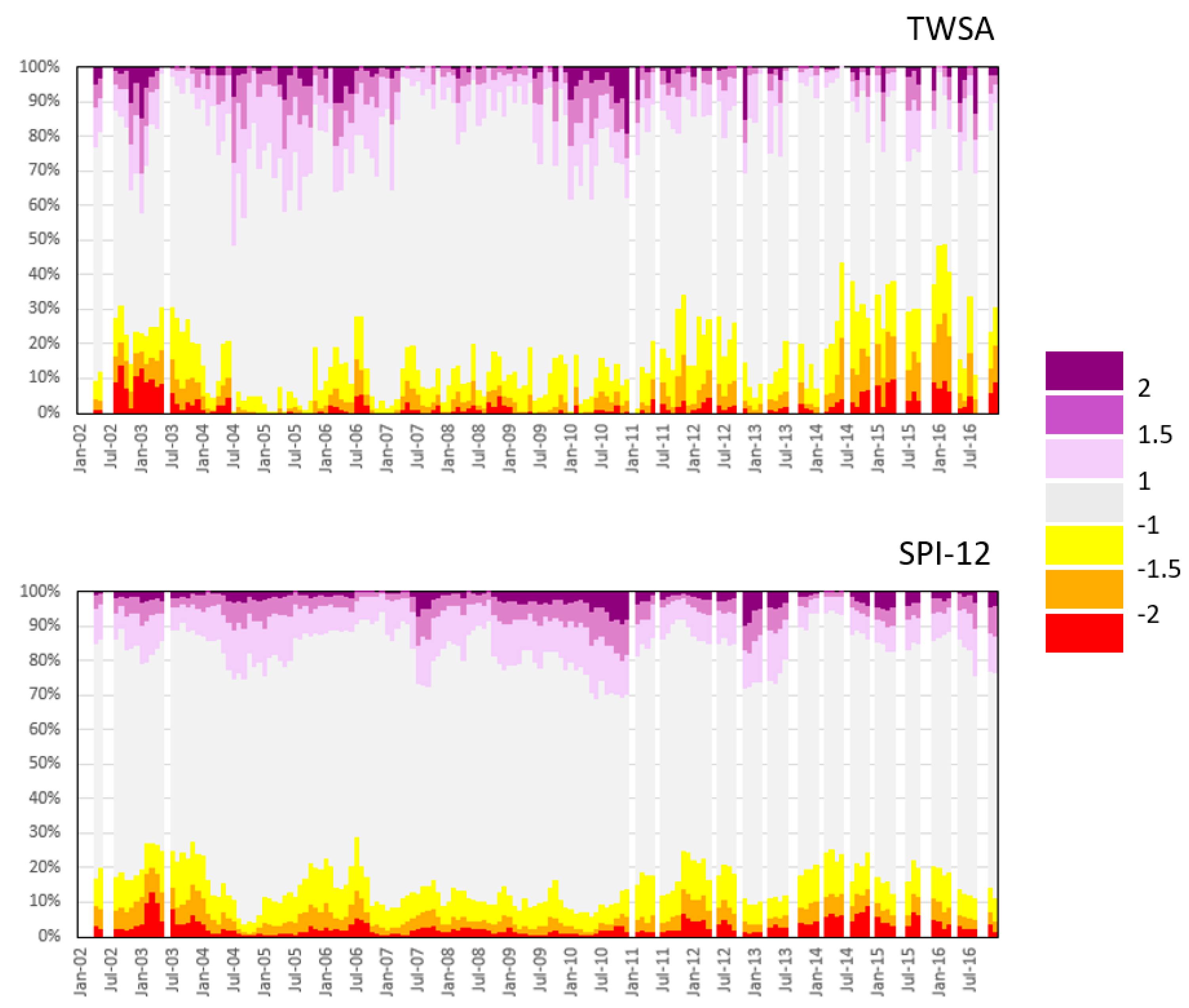
Following the results obtained from the correlation analysis over Europe using SPI-12, an in-depth test focusing only on extreme values was performed in order to understand the capability of this index to specifically reproduce the temporal dynamic of extreme wet and dry conditions as detected by the GRACE-derived TWSA. The plots in Figure 7 show the temporal series of the fraction of cells within each of the seven sub-classes identified in McKee et al. [48] (and outlined in Sub-Section 2.3) for both the TWSA (upper panel) and SPI-12 (lower panel).
These plots show an overall good correspondence between the two datasets, with the major dry periods observed in TWSA in 2003, 2006 and 2012 also reproduced by SPI-12, as well as the major wet periods in 2005 and 2010. The main notable difference between the two time series was in the increasing frequency of dry events captured by TWSA at the end of the observed period in 2016, which was not reproduced by SPI-12. While a possible explanation could be related to the degradation of the GRACE signal right before its decommissioning, this difference was mostly driven by a dry period over Eastern Europe during January–February 2016 that seems to be captured by TWSA but not by SPI-12. It is worth recalling that this was the area where the difference between the local-optimal SPI (SPI-24 and SPI-48) and SPI-12 was statistically significant (see Figure 6).
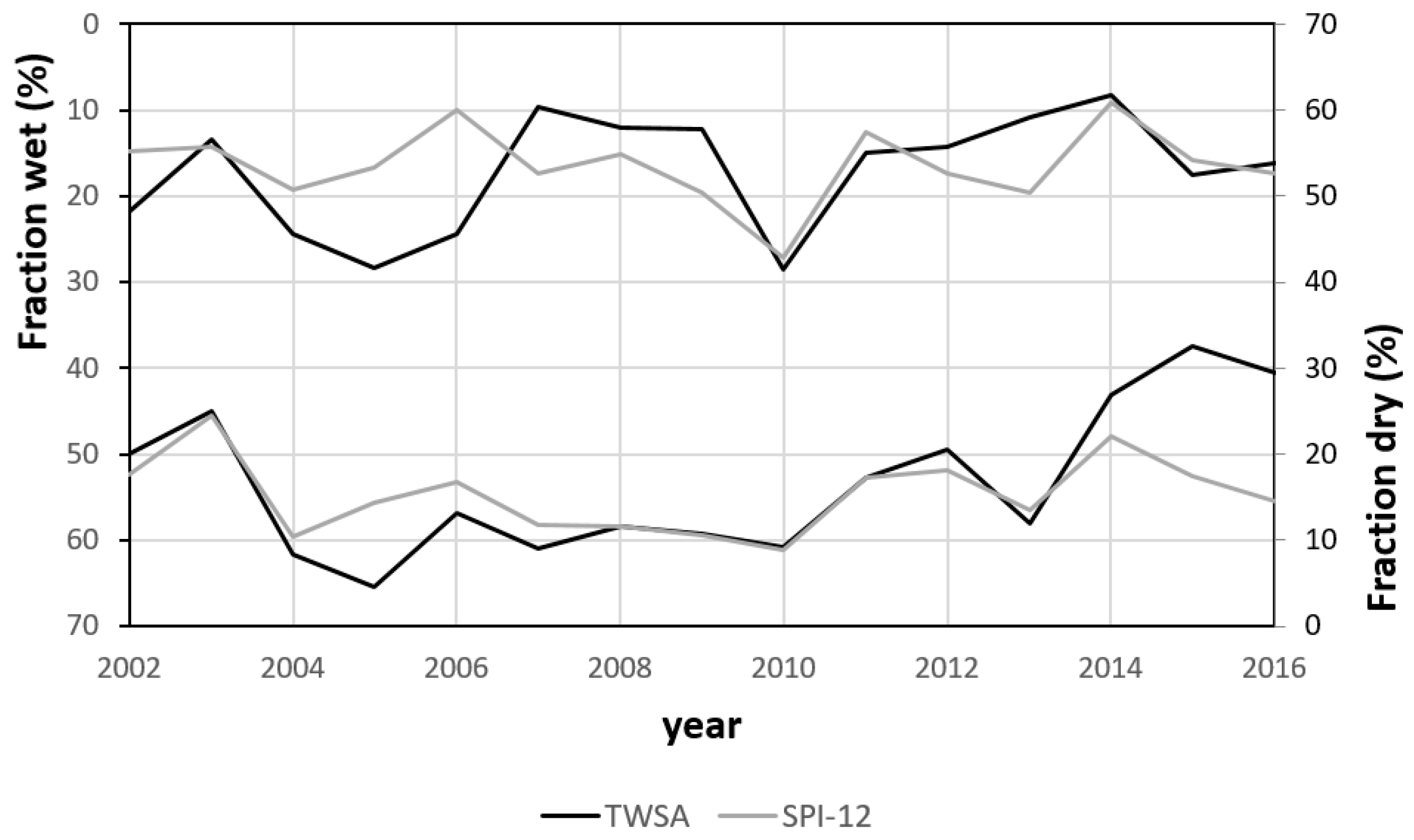
Finally, the data in Figure 8 report a quantitative analysis of the performance on extreme values at year-scale, showing a summary of the total percentage of wet (>1) and dry (<−1) cells for each year according to TWSA and SPI-12. The graph further highlights the overall good agreement between the two datasets in capturing the frequency of both extreme cases, which was particularly true for the dry extremes, for which the SPI-12 seems to reproduce the percentages obtained with the TWSA particularly well (R = 0.70). The only notable exception relevant for drought was represented once again by the dry fraction in the year 2016 (difference > 15%).
4. Summary and Conclusions
Despite the growing availability of local- and continental-scale drought monitoring tools, long-term hydrological droughts remain underrepresented in operational systems, mainly due to the lack of suitable near-real-time datasets, such as groundwater or TWS measurements. While SPI computed over long accumulation periods (i.e., 12 months or longer) is often considered a good proxy for the monitoring of long-term hydrological drought, a comprehensive investigation of the connection between the GRACE-derived TWS and SPI was required to better understand the spatiotemporal traits of such a relationship.
The global-scale analysis performed in this study highlighted the good correlation between the TWS standardised deviation from the climatology (TWSA) and long-term SPI, confirming the potential role of TWSA as a reliable measure of long-term hydrological drought. On average, the SPI-12 showed the highest correlation with TWSA (0.350 ± 0.250), even if a large spatial variability could be observed in the local-optimal SPI. The frequency distribution of the local-optimal SPI values highlighted how SPI-12, SPI-24 and SPI-48 accounted for about 2/3 of the total cells, with a spatial distribution that was characterised by clear patterns, but that could not be easily related to commonly available hydrological characteristics. This complexity in the spatiotemporal response of TWS to variations in precipitation confirmed the value of introducing specific indicators that focus on the monitoring of TWS into operational drought monitoring systems, since a single SPI did not seem to be a reliable proxy of the GRACE-derived TWSA at the global scale.
However, an analysis of the spatial distribution of the correlation coefficients for SPI-12 (i.e., the global-optimal) compared to the local-optimal SPI suggested that over limited areas, such as Europe, a single indicator can be used to successfully capture most of the TWSA dynamic. In more than 90% of cells in Europe, the difference in the correlation between SPI-12 and the local-optimal SPI was not statistically significant (p > 0.05), with an average correlation over Europe (0.42 ± 0.20) that was comparable with the optimal global-average. A specific analysis focused on extreme values also confirmed the capability of SPI-12 to reproduce the extremes observed using TWSA, which was particularly true for the dry values, which were the major focus of drought monitoring.
Overall, the outcomes of this study confirmed the relevance of TWSA within the framework of long-term drought monitoring, as well as the difficulty in capturing its global scale temporal dynamics by simply using classical meteorological drought indices. In fact, even if there was a clear statistically significant correlation between precipitation anomalies (i.e., SPI) and TWSA, the complexity in the hydrological processes that rule the transfer of rainfall into aquifers could not be globally captured by a simple single index. On the contrary, by focusing the analysis on a limited region, such as Europe, it was possible to achieve an acceptable representation of the TWSA by simply using SPI-12. This result represents a key finding for an operational monitoring system, given the relative simplicity of computing SPI-12 compared to TWSA, and the current lack of near-real-time TWS datasets.
In view of the release of GRACE-FO products, the results of this study can be used as a benchmark to evaluate the effectiveness of this brand-new dataset within the context of drought analyses. The outcome that TWSA correlates with any SPI better than with TWS suggests that long time series of TWS data are needed for drought analysis, hinting at a mandatory integration of GRACE and GRACE-FO data for anomaly computation, which raises the question of possible inconsistencies between the two datasets, as well as of the possible impact of the limited length of data records on the reliability of the derived drought events. In addition, the relationships observed between multiple SPI and GRACE products seem robust enough to be considered as a reference for future analogous analyses on GRACE-FO data, allowing the evaluation of the capability of the new dataset to preserve the correlations with SPI observed for its predecessor.
Author Contributions
C.C. processed the data, conducted the analysis and drafted the paper. C.C., P.B. and J.V.V. have worked collaboratively on structuring and reviewing the text, as well as discussing the results.
Funding
This research received no external funding.
Acknowledgments
The authors thank the NASA Jet Propulsion Laboratory PO.DAAC for making the GRACE dataset freely available, as well as the entire JRC drought team for processing and maintaining the SPI dataset. Outputs of this study can be requested through the EDO/GDO web portals.
Conflicts of Interest
The authors declare no conflict of interest.
References
- Wilhite, D.A. Drought as a Natural Hazard: Concepts and Definitions; A Global Assessment; Rourledge: Abingdon-on-Thames, UK, 2000; pp. 3–18. [Google Scholar]
- Western Governors’ Association. Creating a Drought Early Warning System for the 21th Century: The National Integrated Drought Information System; Report; Western Governors’ Association: Denver, CO, USA, 2004; p. 13. Available online: https://www.drought.gov/drought/sites/drought.gov.drought/files/media/whatisnidis/Documents/200406_WGA_NIDIS_Report.pdf (accessed on 12 August 2019).
- European Commission. Water Scarcity and Droughts: In-Depth Assessment; European Commission, DG Environment: Brussels, Belgium, 2007; p. 93. Available online: http://ec.europa.eu/environment/water/quantity/pdf/comm_droughts/2nd_int_report.pdf (accessed on 12 August 2019).
- Bryant, E.A. Natural Hazards; Cambridge University Press: Cambridge, UK, 1991. [Google Scholar]
- Pischke, F.; Stefanski, R. Drought management policies—From global collaboration to national action. Water Policy 2016, 18, 228–244. [Google Scholar] [CrossRef]
- Wilhite, D.A.; Pulwarty, R.S. Drought and Water Crises: Lessons Learned and the Road Ahead. In Drought and Water Crises: Science, Technology, and Management; Wilhite, D.A., Ed.; CRC Press: Boca Raton, FL, USA, 2005; pp. 389–398. [Google Scholar]
- WMO (World Meteorological Organization); GWP (Global Water Partnership). National Drought Policy Guidelines: A Template for Action (D.A. Wilhite); Integrated Drought Management Programme (IDMP) Tools and Guidelines Series 1; WMO: Geneva, Switzerland; GWP: Stockholm, Sweden, 2014. [Google Scholar]
- Sepulcre-Canto, G.; Horion, S.; Singleton, A.; Carrao, H.; Vogt, J. Development of a combined drought indicator to detect agricultural drought in Europe. Nat. Hazards Earth Syst. Sci. 2012, 12, 3519–3531. [Google Scholar] [CrossRef]
- Cammalleri, C.; Vogt, J.; Salamon, P. Development of an operational low-flow index for hydrological drought monitoring over Europe. Hydrol. Sci. J. 2017, 62, 346–358. [Google Scholar] [CrossRef]
- Bachmair, S.; Stahl, K.; Collins, K.; Hannaford, J.; Acreman, M.; Svoboda, M.; Knutson, C.; Smith, K.H.; Wall, N.; Fuchs, B.; et al. Drought indicators revised: The need for a wider consideration of environment and society. Wiley Interdisc. Rew. Water 2016, 3, 516–536. [Google Scholar] [CrossRef]
- Ojha, R.; Ramadas, M.; Govindaraju, R.S. Current and future challenges in groundwater. I: Modeling and management of resources. J. Hydrol. Eng. 2015, 20, A4014007. [Google Scholar] [CrossRef]
- Chang, T.J.; Teoh, C.B. Use of the kriging method for studying characteristics of ground water droughts. J. Am. Water Resour. Ass. 1995, 31, 1001–1007. [Google Scholar] [CrossRef]
- Shahid, S.; Hazarika, M.K. Groundwater drought in the northwestern districts of Bangladesh. Water Resour. Manag. 2010, 24, 1989–2006. [Google Scholar] [CrossRef]
- Bloomfield, J.P.; Marchant, B.P. Analysis of groundwater drought building on the standardized precipitation index approach. Hydrol. Earth Syst. Sci. 2013, 17, 4769–4787. [Google Scholar] [CrossRef]
- Tapley, B.D.; Bettadpur, S.; Ries, J.C.; Thompson, P.F.; Watkins, M.M. GRACE measurements of mass variability in the Earth System. Science 2004, 305, 503–505. [Google Scholar] [CrossRef] [PubMed]
- Wahr, J.; Swenson, S.; Velicogna, I. Accuracy of GRACE mass estimates. Geophys. Res. Lett. 2006, 33, L06401. [Google Scholar] [CrossRef]
- Houborg, R.; Rodell, M.; Li, B.; Reichle, R.; Zaitchik, B.F. Drought indicators based on model-assimilated Gravity Recovery and Climate Experiment (GRACE) terrestrial water storage observations. Water Resour. Res. 2012, 48, W07525. [Google Scholar] [CrossRef]
- Li, B.; Rodell, M. Evaluation of a model-based groundwater drought indicator in the conterminous U.S. J. Hydrol. 2015, 526, 78–88. [Google Scholar] [CrossRef] [Green Version]
- Zaitchik, B.F.; Rodell, M.; Reichle, R.H. Assimilation of GRACE terrestrial water storage into a land surface model: Results for the Mississippi River basin. J. Hydrometeorol. 2008, 9, 535–548. [Google Scholar] [CrossRef]
- Güntner, A. Improvement of global hydrological models using GRACE data. Surv. Geophys. 2008, 29, 375–397. [Google Scholar] [CrossRef]
- Hasegawa, T.; Fukuda, Y.; Yamamoto, K. The 2006 Australian drought detected by GRACE. In From Headwaters to the Ocean; Taniguchi, M., Ed.; Taylor and Francis: London, UK, 2009; pp. 363–367. [Google Scholar]
- Schmidt, R.; Schwintzer, P.; Flechtner, F.; Reigber, C.; Günter, A.; Döll, P.; Ramilien, G.; Cazenave, A.; Petrovic, S.; Jochmann, H.; et al. GRACE observations of changes in continental water storage. Glob. Planet Chang. 2006, 50, 112–126. [Google Scholar] [CrossRef]
- Ma, S.; Wu, Q.; Wang, J.; Zhang, S. Temporal evaluation of regional drought detected from GRACE TWSA and CCI SM in Yunnan Province, China. Remote Sens. 2017, 9, 1124. [Google Scholar] [CrossRef]
- Sinha, D.; Syed, T.H.; Famiglietti, J.S.; Reager, J.T.; Thomas, R.C. Characterizing drought in India using GRACE observations of terrestrial storage deficit. J. Hydrometeorol. 2017, 18, 381–396. [Google Scholar] [CrossRef]
- Zhao, M.; Geruo, A. Satellite observations of regional drought severity in the continental United States using GRACE-based terrestrial water storage changes. J. Climate 2017, 30, 6297–6308. [Google Scholar] [CrossRef]
- Yirdaw, S.Z.; Snelgrove, K.R.; Agboma, C.O. GRACE satellite observations of terrestrial moisture changes for drought characterization in the Canadian prairie. J. Hydrol. 2008, 356, 84–92. [Google Scholar] [CrossRef]
- Scanlon, B.R.; Zhang, Z.; Reedy, R.C.; Pool, D.R.; Save, H.; Long, D.; Chen, J.; Wolock, D.M.; Conway, B.D.; Winester, D. Hydrologic implications of GRACE satellite data in the Colorado river basin. Water Resour. Res. 2015, 51, 9891–9903. [Google Scholar] [CrossRef]
- Chen, J.L.; Wilson, C.R.; Tapley, B.D.; Yang, Z.L.; Niu, G. 2005 drought event in the Amazon River basin as measured by GRACE and estimated by climate models. J. Geophys. Res. 2009, 114, B05404. [Google Scholar] [CrossRef]
- Long, D.; Scanlon, B.R.; Longuevergne, L.; Sun, A.-Y.; Fernando, D.N.; Himanshu, S. GRACE satellites monitor large depletion in water storage in response to the 2011 drought in Texas. Geophys. Res. Lett. 2013, 40, 3395–3401. [Google Scholar] [CrossRef]
- Van Loon, A.F.; Kumar, R.; Mishra, V. Testing the use of standardised indices and GRACE satellite data to estimate the European 2015 groundwater drought in near-real time. Hydrol. Earth Syst. Sci. 2017, 21, 1947–1971. [Google Scholar] [CrossRef] [Green Version]
- Zhang, Z.; Chao, B.F.; Chen, J.; Wilson, C.R. Terrestrial water storage anomalies of Yangtze River basin droughts observed by GRACE and connections with ENSO. Global Planet. Change 2015, 126, 35–45. [Google Scholar] [CrossRef]
- Thomas, A.C.; Reager, J.T.; Famiglietti, J.S.; Rodell, M.A. GRACE-based water storage deficit approach for hydrological drought characterization. Geophys. Res. Lett. 2014, 41, 1537–1545. [Google Scholar] [CrossRef]
- AghaKouchak, A.; Farahmand, A.; Melton, F.S.; Teixeira, J.; Anderson, M.C.; Wardlow, B.D.; Hain, C.R. Remote sensing of drought: Progress, challenges, and opportunities. Rev. Geophys. 2015, 53, 452–480. [Google Scholar] [CrossRef]
- Humphrey, V.; Gudmundsson, L.; Seneviratne, S.I. Asessing global water storage variability from GRACE: Trends, seasonal cycle, subseasonal anomalies and extremes. Surv. Geophys. 2016, 37, 357–395. [Google Scholar] [CrossRef]
- Sun, A.Y.; Scanlon, B.R.; AghaKouchak, A.; Zhang, Z. Using GRACE satellite gravimetry for assessing large-scale hydrologic extremes. Remote Sens. 2017, 9, 1287. [Google Scholar] [CrossRef]
- Raziei, T.; Saghafian, B.; Paulo, A.A.; Pereira, L.S.; Bordi, I. Spatial patterns and temporal variability of drought in western Iran. Water Resour. Manag. 2008, 27, 1661–1674. [Google Scholar] [CrossRef]
- Thomas, T.; Jaiswal, R.K.; Nayak, P.C.; Ghosh, N.C. Comprehensive evaluation of the changing drought characteristics in Brundelkhand region of Central India. Meteorol. Atmos. Phys. 2015, 127, 163–182. [Google Scholar] [CrossRef]
- Joetzjer, E.; Douville, H.; Delire, C.; Ciais, P.; Decharme, B.; Tyteca, S. Hydrologic benchmarking of meteorological drought indices at interannual to climate change timescales: A case study over the Amazon and Mississippi river basins. Hydrol. Earth Syst. Sci. 2013, 17, 4885–4895. [Google Scholar] [CrossRef]
- Bloomfield, J.P.; Marchant, B.P.; Bricker, S.H.; Morgan, R.B. Regional analysis of groundwater droughts using hydrograph classification. Hydrol. Earth Syst. Sci. 2015, 19, 4327–4344. [Google Scholar] [CrossRef] [Green Version]
- Kumar, R.; Musuuza, J.L.; Van Loon, A.F.; Teuling, A.J.; Barthel, R.; Ten Broek, J.; Mai, J.; Samaniego, L.; Attinger, S. Multiscale evaluation of the Standardized Precipitation Index as a groundwater drought indicator. Hydrol. Earth Syst. Sci. 2016, 20, 1117–1131. [Google Scholar] [CrossRef] [Green Version]
- Changnon, S.A., Jr. Detecting Drought Conditions in Illinois; Illinois State Water Survey Champaign, Circular 169: Champaign, IL, USA, 1987; 36p. [Google Scholar]
- Wahr, J.; Swenson, S.; Zlotnicki, V.; Velicogna, I. Time-variable gravity from GRACE: First results. Geophys. Res. Lett. 2004, 31, L11501. [Google Scholar] [CrossRef]
- Landerer, F.W.; Swenson, S.C. Accuracy of scaled GRACE terrestrial water storage estimates. Water Resour. Res. 2012, 48, W04531. [Google Scholar] [CrossRef]
- Wahr, J.; Molenaar, M.; Bryan, F. Time-variability of the Earth’s gravity field: Hydrological and oceanic effects and their possible detection using GRACE. J. Geophys. Res. 1998, 103, 30205–30230. [Google Scholar] [CrossRef]
- Swenson, S.; Wahr, J. Post-processing removal of correlated errors in GRACE data. Geophys. Res. Lett. 2006, 33, L08402. [Google Scholar] [CrossRef]
- Geruo, A.; Wahr, J.; Zhong, S. Computations of the viscoelastic response of a 3-D compressible Earth to surface loading: An application to Glacial Isostatic Adjustment in Antarctica and Canada. Geophys. J. Int. 2013, 192, 557–572. [Google Scholar]
- Klees, R.; Zapreeva, E.A.; Winsemius, H.C.; Savenije, H.H.G. The bias in GRACE estimates of continental water storage variations. Hydrol. Earth Syst. Sci. 2007, 11, 1227–1241. [Google Scholar] [CrossRef] [Green Version]
- McKee, T.B.; Doesken, N.J.; Kleist, J. The relationship of drought frequency and duration to time scale. In Proceedings of the 8th Conference on Applied Climatology, Anaheim, CA, USA, 17–22 January 1993; American Meteorological Society: Boston, MA, USA, 1993; pp. 179–184. [Google Scholar]
- WMO, World Meteorological Organization. Standardized Precipitation Index User Guide; Svoboda, M., Hayes, M., Wood, D., Eds.; WMO-No. 1090; World Meteorological Organization: Geneva, Switzerland, 2012; 16p. [Google Scholar]
- Thom, H.C.S. A note on the Gamma distribution. Monthly Weath. Rev. 1958, 86, 117–122. [Google Scholar] [CrossRef]
- Wu, H.; Svoboda, M.D.; Hayes, M.J.; Wilhite, D.A.; Wen, F. Appropriate application of the standardized precipitation index in arid locations and dry seasons. Int. J. Climatol. 2006, 27, 65–79. [Google Scholar] [CrossRef]
- Stoelzle, M.; Stahl, K.; Morhard, A.; Weiler, M. Streamflow sensitivity to drought scenarios in catchments with different geology. Geophys. Res. Lett. 2014, 41, 6174–6183. [Google Scholar] [CrossRef]
- Steiger, J.H. Tests for comparing elements of a correlation matrix. Psychol. Bull. 1980, 87, 245–251. [Google Scholar] [CrossRef]
- Leander, R.; Buishand, T.A. Resampling of regional climate model output for the simulation of the extreme river flows. J. Hydrol. 2007, 332, 487–496. [Google Scholar] [CrossRef]
Figure 1.
Global-average R between different SPI-n vs. TWS (black line with circles) and TWSA (grey line with squares).
Figure 1.
Global-average R between different SPI-n vs. TWS (black line with circles) and TWSA (grey line with squares).

Figure 2.
Percentage changes in the global-average R between SPI-n and TWSA for different time lag values compared to the outcome for no lag (as reported in Figure 1).
Figure 2.
Percentage changes in the global-average R between SPI-n and TWSA for different time lag values compared to the outcome for no lag (as reported in Figure 1).

Figure 3.
Spatial distribution of the maximum R between SPI and TWSA obtained from the optimal SPI-n. Masked cells (where liquid rainfall was <100 mm annum) are represented in grey.
Figure 3.
Spatial distribution of the maximum R between SPI and TWSA obtained from the optimal SPI-n. Masked cells (where liquid rainfall was <100 mm annum) are represented in grey.

Figure 4.
Spatial distribution of the SPI accumulation period returning the maximum R between SPI and TWSA. Masked cells (where liquid rainfall was <100 mm annum) are represented in grey.
Figure 4.
Spatial distribution of the SPI accumulation period returning the maximum R between SPI and TWSA. Masked cells (where liquid rainfall was <100 mm annum) are represented in grey.

Figure 5.
Statistics of the optimal SPI. (a) Average R values for all the cells with the same local-optimal SPI value. (b) Frequency distribution of the local-optimal SPI values at the global scale.
Figure 5.
Statistics of the optimal SPI. (a) Average R values for all the cells with the same local-optimal SPI value. (b) Frequency distribution of the local-optimal SPI values at the global scale.

Figure 6.
Spatial distribution of the R values corresponding to the relationship between SPI-12 and TWSA (main panel). The striped cells are those where there was a statistically significant difference (p ≤ 0.05) between the local-optimal (see Figure 3) and the SPI-12 R values. The map in the lower-left corner highlights the outcomes over Europe, whereas the lower-right panel shows the frequency distribution of the R values over Europe.

Figure 7.
Time series of the fraction of cells over Europe within each of the seven sub-classes identified in [48] (see Section 2.3). The upper panel reports the data for TWSA, whereas the lower panel shows the results for SPI-12.
Figure 7.
Time series of the fraction of cells over Europe within each of the seven sub-classes identified in [48] (see Section 2.3). The upper panel reports the data for TWSA, whereas the lower panel shows the results for SPI-12.

Figure 8.
Time series of the year-average percentage of dry (on the right-side axis) and wet (on the left-side axis, inverted) cells over Europe according to TWSA (black line) and SPI-12 (grey line).
Figure 8.
Time series of the year-average percentage of dry (on the right-side axis) and wet (on the left-side axis, inverted) cells over Europe according to TWSA (black line) and SPI-12 (grey line).

© 2019 by the authors. Licensee MDPI, Basel, Switzerland. This article is an open access article distributed under the terms and conditions of the Creative Commons Attribution (CC BY) license (http://creativecommons.org/licenses/by/4.0/).
Share and Cite
MDPI and ACS Style
Cammalleri, C.; Barbosa, P.; Vogt, J.V. Analysing the Relationship between Multiple-Timescale SPI and GRACE Terrestrial Water Storage in the Framework of Drought Monitoring. Water 2019, 11, 1672. https://doi.org/10.3390/w11081672
AMA Style
Cammalleri C, Barbosa P, Vogt JV. Analysing the Relationship between Multiple-Timescale SPI and GRACE Terrestrial Water Storage in the Framework of Drought Monitoring. Water. 2019; 11(8):1672. https://doi.org/10.3390/w11081672
Chicago/Turabian StyleCammalleri, Carmelo, Paulo Barbosa, and Jürgen V. Vogt. 2019. "Analysing the Relationship between Multiple-Timescale SPI and GRACE Terrestrial Water Storage in the Framework of Drought Monitoring" Water 11, no. 8: 1672. https://doi.org/10.3390/w11081672
Note that from the first issue of 2016, this journal uses article numbers instead of page numbers. See further details here.