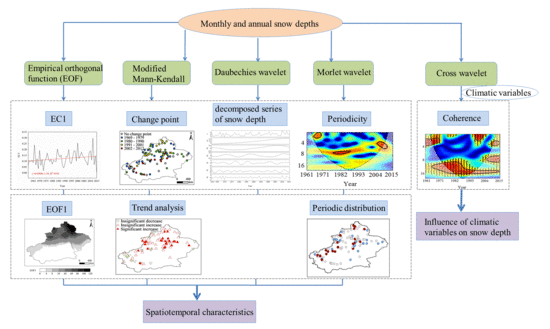
Spatiotemporal Variability of Monthly and Annual Snow Depths in Xinjiang, China over 1961–2015 and the Potential Effects


1
College of Water Resources and Architecture Engineering, Northwest A&F University, Yangling 712100, China
2
Key Lab of Agricultural Water and Soil Engineering of Education Ministry, Northwest Agriculture and Forestry University, Yangling 712100, China
3
Xinjiang Meteorological Observatory, Urumqi 830002, China
*
Author to whom correspondence should be addressed.
Water 2019, 11(8), 1666; https://doi.org/10.3390/w11081666
Submission received: 15 July 2019
/
Revised: 26 July 2019
/
Accepted: 6 August 2019
/
Published: 12 August 2019
(This article belongs to the Section Hydrology)
Abstract
:The spatiotemporal variability of snow depth supplies important information for snow disaster prevention. The monthly and annual snow depths and weather data (from Xinjiang Meteorological Observatory) at 102 meteorological stations in Xinjiang, China over 1961–2015 were used to analyze the spatiotemporal characteristics of snow depths from different aspects. The empirical orthogonal function (EOF), the modified Mann–Kendall method, Morlet wavelet, Daubechies wavelet decomposition and cross wavelet transform were applied to investigate the trend and significance, spatial structure, periods, decomposed series and coherence of monthly and annual snow depths. The results indicated that: (1) The value of EOF first spatial mode (EOF1) of the monthly and annual snow depths in north Xinjiang were larger than south Xinjiang, indicating greater variability of snow depths in north Xinjiang. (2) The change points of annual snow depth mainly occurred during 1969–1979 and 1980–1990. The annual snow depth of most sites showed increasing trends, but with different slope magnitudes. (3) The sites that had main periods of 2–8 and 9–14 years of monthly and annual snow depths (detected by the Morlet wavelet) mainly distributed in northern Xinjiang. The sites that had main periods of 15–20 years of monthly and annual snow depths mainly distributed in southwestern Xinjiang. (4) By using the Daubechies wavelet, the decomposed annual snow depth in entire Xinjiang tended to increase. (5) Through the cross wavelet transform, annual snow depths in entire Xinjiang had good correlations with annual precipitation or relative humidity, and showed a low negative correlation with minimum temperature or sunshine hours. In conclusion, the monthly and annual snow depths had comprehensive spatiotemporal variability but had overall increasing trend during 1961–2015.
1. Introduction
Snow water is an important freshwater resource on Earth [1]. Snow cover is one of the important factors affecting the global climate [2]. Snow is also the most active and widely covered element of the cryosphere. It not only profoundly affects energy balance of the Earth’s surface, but also plays a prominent role in the hydrological cycle. The high reflectivity and the low conductivity of snowpack affect the energy exchange between the land–atmosphere system [3,4,5]. Snow parameters include snowfall, snow depth, snow density, snow pressure, snow area, snow temperature, snow water equivalent, etc. Snow depth is an indispensable indicator for estimating snow water equivalent, calculating surface radiation and water budget, and simulating snowmelt runoff in spring [6].
There have been several research projects on spatial and temporal variation analysis, simulation and remote sensing analysis of snow depth, conducted at daily, monthly, or annual scales and in different parts of the world [7,8]. Liu et al. [9] used wavelet analysis to analyze the periodic characteristics of maximum snow depth in northern Xinjiang over 1961–2008. They found that the maximum snow depth had a main period of 7–11 years in northern Xinjiang. Hu et al. [10] analyzed the correlation coefficient between the annual snow depth and the annual precipitation (or average temperature) in Xinjiang over 1960–2011. The annual snow depth had a good correlation with the annual precipitation, but a low correlation with the average temperature. Xu et al. [11] used a linear model to investigate the spatiotemporal characteristics of daily snow depth and the snow-cover days in the Qinghai–Tibetan Plateau over 1961–2010. They revealed that snow cover was controlled by multiple climate factors rather than a single variable. Ding et al. [6] used the modified Mann–Kendall test to analyze trends and significance of daily snow depth at 105 stations (spread in the whole area) in Xinjiang, China over 1961–2013 and indicated upward trends at 86 stations. Brun et al. [7] used the ISBA/Crocus (a detailed snowpack model coupled with a soil model) and forcing meteorological data from Interim Re-Analysis and Princeton University Global Forcing dataset to perform snow simulation, and compared the daily snow depth results with observed values over 14 years across more than 250 stations in northern Eurasia. They concluded that the best simulation was obtained with Interim Re-Analysis. Che et al. [12] studied the spatiotemporal distribution of seasonal snow depth derived from passive microwave satellite remote-sensing data in China over 1987–2006. They found that snow depth in China showed significant inter-annual variation, with a weak increasing trend. Although different research has revealed the changes of snow depth in partial or entire China, the variability (including spatial and temporal variations, periodical changes, and correlations with environmental or climatic variables) of monthly and annual snow depths in Xinjiang have not been systematically investigated by combining different spatiotemporal analysis methods.
A number of the methods could reveal the internal spatiotemporal structures of the hydrological time series, such as stochastic method, singular value decomposition, canonical correlation, cluster analysis, empirical mode decomposition [13], artificial neural networks [14], support vector machine [15], spectrum analysis [16], wavelet analysis [17], empirical orthogonal function (EOF) [18], etc. The EOF method condenses the spatiotemporal information, reveals spatial and systematic structures, and identifies dominant variation patterns of series. It has been applied for soil water content variability in the Canadian Prairie pothole region [19], water quality variation of Nakdong River, Korea [20], terrestrial water storage change in the Tarim River basin, China [21], daily snow depth changes in Xinjiang, China [6] and other hydrological variables [22,23]. The wavelet analysis includes continuous and discrete ones. The former determines both the scale contents of a signal and temporal variations. The latter is often used to decompose a series into sub-signals at wavelet and decomposition level, and then guide wavelet decomposition, wavelet de-noising [24], wavelet aided complexity description and wavelet aided hydrologic forecasting analysis [25]. The wavelet transform has been extensive applied. For example, Torrence and Compo [26] operated continuous wavelet transform and Labat [27] and Schaefli et al. [28] conducted overviews or applications of wavelet analysis from different aspects or research fields. Rashid et al. [29] used continuous wavelet transform to assess trends in point rainfall. Kuang et al. [30] used continuous wavelet transform to reveal the multiscale structure, break point, change and distribution of periodic variation in runoff series of the Yangtze River basin in China. It was shown that the wavelet analysis could reveal the spatiotemporal changes of hydrological series very well. However, continuous and discrete wavelet analysis have been seldom applied in detailed snow depth variability research by combining with other time-series analysis methods.
Until present, not much research has combined EOF with trend tests and different wavelet analysis methods to analyze the spatiotemporal variability of monthly and annual snow depths in Xinjiang, China. This research aims to: (i) analyze the spatiotemporal variability structures and trends in the monthly and annual snow depths at 102 weather stations in Xinjiang, China over 1961–2015 using EOF, the trend test and three wavelet methods, (ii) reveal the periods of daily and annual snow depths both in time and frequency domain, and (iii) find the key climatic variables that affected annual snow depths. The combination of different methods would reveal the spatiotemporal structures of monthly and annual snow depths in Xinjiang in more detail.
The organization of this paper is as follows. The details about the study area and data sources as well as procedures of four methods for analyzing the spatiotemporal variability of snow depth is described in Section 2. The results related to spatial and temporal variation characteristics of snow depth and several key climatic variables that affected snow depth is introduced in Section 3. The potential impacts of changes in snow depth is discussed in Section 4. Section 5 provides concise conclusions about the spatiotemporal variability of snow depth.
2. Materials and Methods
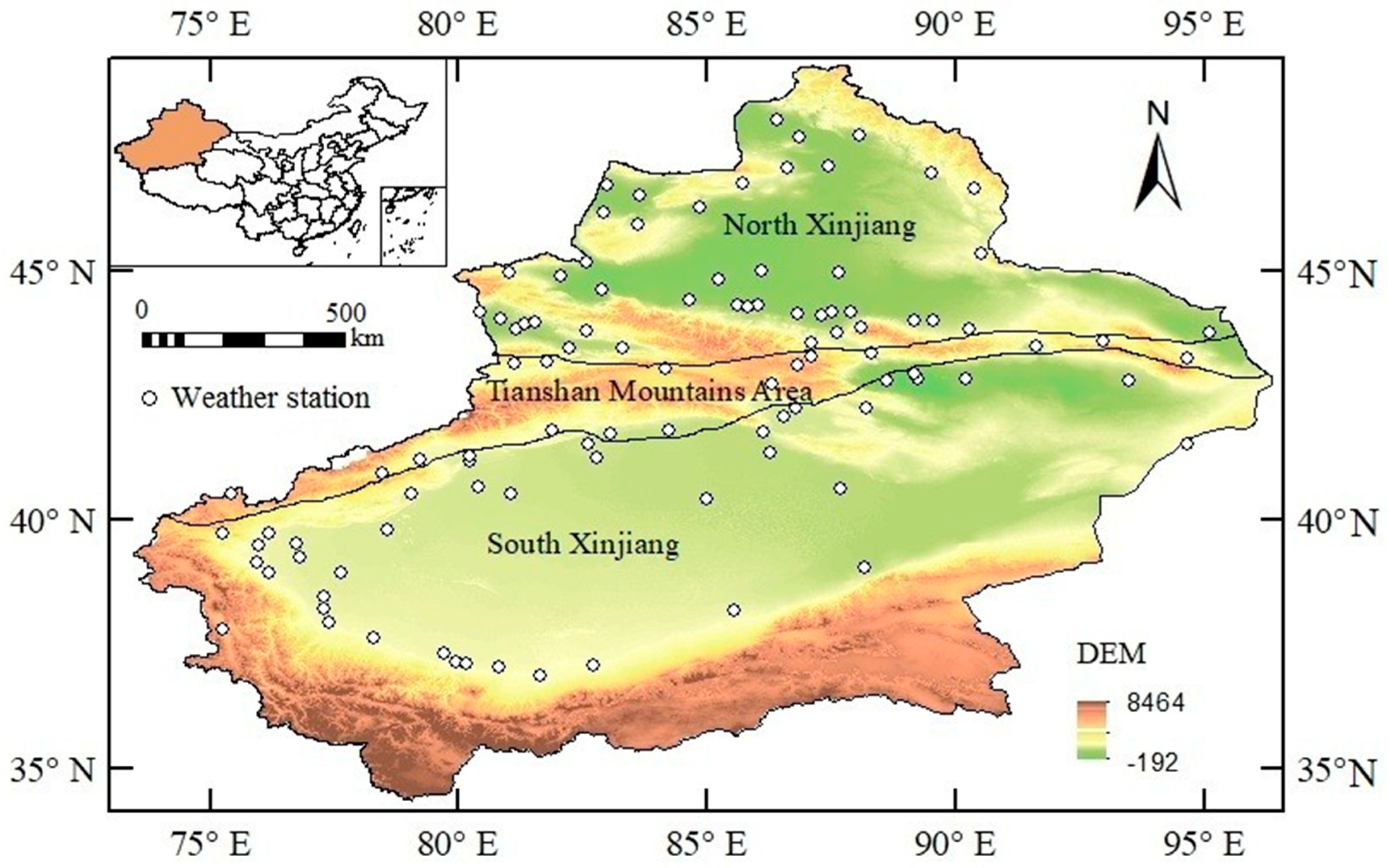
2.1. Study Area and Datasets
Xinjiang Uygur Autonomous region is located in the hinterland of Asia–Europe and in the northwestern part of China with latitude range of 32°22′ N~49°33′ N. The longitude range is 73°21′ E~96°21′ E and altitude range is −192–8464 m. Its total area is 1,665,900 km2, accounting for one sixth of China’s total land area. The terrain of Xinjiang is dominated by several mountains, hills and basins. Its topographies are commonly known as “three mountains with two basins”, namely Altai Mountain (in the north), Kunlun Mountain (in the south), Tianshan Mountain (in the central part), Tarim and the Junggar Basins [31,32]. Xinjiang is far away from any sea, with low precipitation, high evaporation and dry climate [33]. It is a typical arid and semi-arid inland region with insufficient surface water resources, but its seasonal snow water resources are abundant, accounting for one third of the total snow resources in the country. The area of permanent snow and glaciers in Xinjiang was larger than 20,000 km2, accounting for 41% of the country’s snow and ice area. North Xinjiang and most of southern Xinjiang have perennial snowfall [6]. The snow-cover in northern Xinjiang reaches a maximum of 210 days, but is less than 60 days in south Xinjiang. There are more snowfall days in northern Xinjiang, for example the Turkut station (75.4° E, 40.5° N, and 3504.4 m above sea level) reached 136 days of snow-cover duration. Snowstorms, blizzards and avalanches in pasturing areas have occurred frequently in Xinjiang, causing serious consequences and disasters [34]. Increasing snow-related concerns and topics in Xinjiang has been focused on in recent years.
The daily snow depth and weather data over 1961–2015 at the 102 stations in Xinjiang were obtained from Xinjiang Meteorology Bureau of China. The snow year begins from 1 October and ends on 30 September of the next year. The elevations of the selected sites range between −192 and 8464 m above sea level. Data quality control has been strictly conducted. Monthly and annual snow depths (or climatic variables) were obtained from averaged daily values. Snow depth was measured with a ruler, three times one day to provide an average value. Weather data include the climatic variables that may affects snowfall, i.e., precipitation, minimum temperature (cold conditions), relative humidity and sunshine hours. The quality and reliability of the climatic variables was investigated through non-parametric tests. Randomness, homogeneity and absence of trends were tested using the Kendall autocorrelation test, the Mann–Kendall trend test and the homogeneity tests of Mann–Whitney for mean and variance [35].
The site distribution and the elevation variations in Xinjiang were mapped in ArcGIS 10.2 (Figure 1).
2.2. Methods
2.2.1. Mann–Whitney Test
The Mann–Whitney test compares two independent samples that are not paired and is used for checking the difference between the two data sets. First, regardless of the grouping, all the data is sorted. The smallest value rank is 1 and the largest is the total observation number. If the data have the same value, the same rank is obtained. The ranks of the same values are the average of their ranks. If the difference between ranks of two groups is large, a smaller significance level (p-value) is obtained and there is a significant difference between the two groups [36]. The SPSS 24.0 software was applied to conduct the Mann–Whitney test.
2.2.2. Empirical Orthogonal Function
The empirical orthogonal function (EOF) has a linear transformation of the original data, produces a new set of orthogonal functions and excludes redundant information [37]. For a spatiotemporal field, the EOF form is:
where φij is the i-th component of the j-th random vector for the centralized and normalized data, i (= 1,..., m) is the site and m is the total number of sites (102); j = (1,..., n) is the time series and n is the serial length (55); Uki is the weight coefficient representing the contribution of the i-th site in the k-th component, Uki vary between the series but are constant in time [38]; is the time dependent function of the i-th site in the k-th component of expansion.
2.2.3. Trend, Significance and Slope of Snow Depth
The modified Mann–Kendall (MMK) method [39] based on a non-parametric analysis [40,41] is used to robustly test trends in the annual mean snow depth over 1961–2015. The MMK test considers the effects of serial self-correlation on the statistic (Z) tested by the original Mann–Kendall method. A modified statistic ZM is obtained using a correction factor—ns, written as follows:
where rjj is the serial self-correlation coefficient given a lag jj, n is serial length.
Both Z and ZM follow a standard normal distribution under the hypothesis of no trend. The null hypothesis is rejected if > 1.96 at a 0.05 confidence level. If ZM is positive (negative), the tested series have an upward (downward) trend [42].
2.2.4. Wavelet Analysis
Wavelet analysis uses a cluster of wavelet functions to indicate a signal [45,46]. Three wavelet analysis methods including continuous (multi-Morlet) wavelet transform, discrete (Daubechies) wavelet transform and cross wavelet transform were applied in this research. Detailed descriptions of the theory are as follows. A continuous wavelet transform is performed using the Morlet wavelet basis .
The Daubechies wavelet is a wavelet function constructed by Inrid Daubechies [47]. It is used to perform a differential operation of one-dimensional discrete time series. The studied series is decomposed up to the log2n layer, where n is the number of samples (n = 55). Only db1 has explicit expressions. Other wavelets provide more efficient analysis and synthesis than db1. Snow depth data is decomposed by Daubechies to the fifth layer and the db5 wavelet is selected to perform further analysis.
The cross wavelet analysis is a combination of cross-spectral analysis and wavelet transform. Cross-wavelet transform and the wavelet coherence provide information about the relation between time series [48]. To measure intrinsic correlation between the wavelet spectra of two time-series X (snow depth) and Y (climatic variables), the cross-wavelet transform is written as [49]:
The cross-wavelet power is calculated as . Furthermore, the phase shift between the analyzed series is calculated as the angle of the complex part of the cross-wavelet transform as arg(WX,Y). By normalizing the cross-wavelet transform the wavelet coherence is obtained.
The MATLAB 17.0 software (MathWorks, Natick, MA, USA) was applied to perform the mathematical analysis.
3. Results
3.1. Spatiotemporal Variations of Monthly and Annual Snow Depths
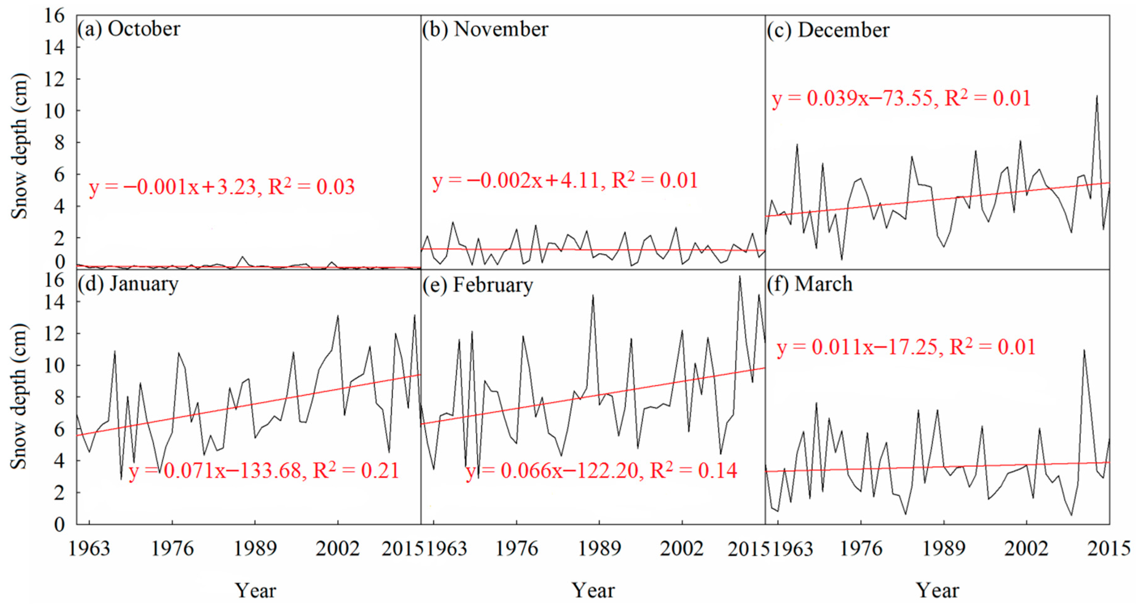
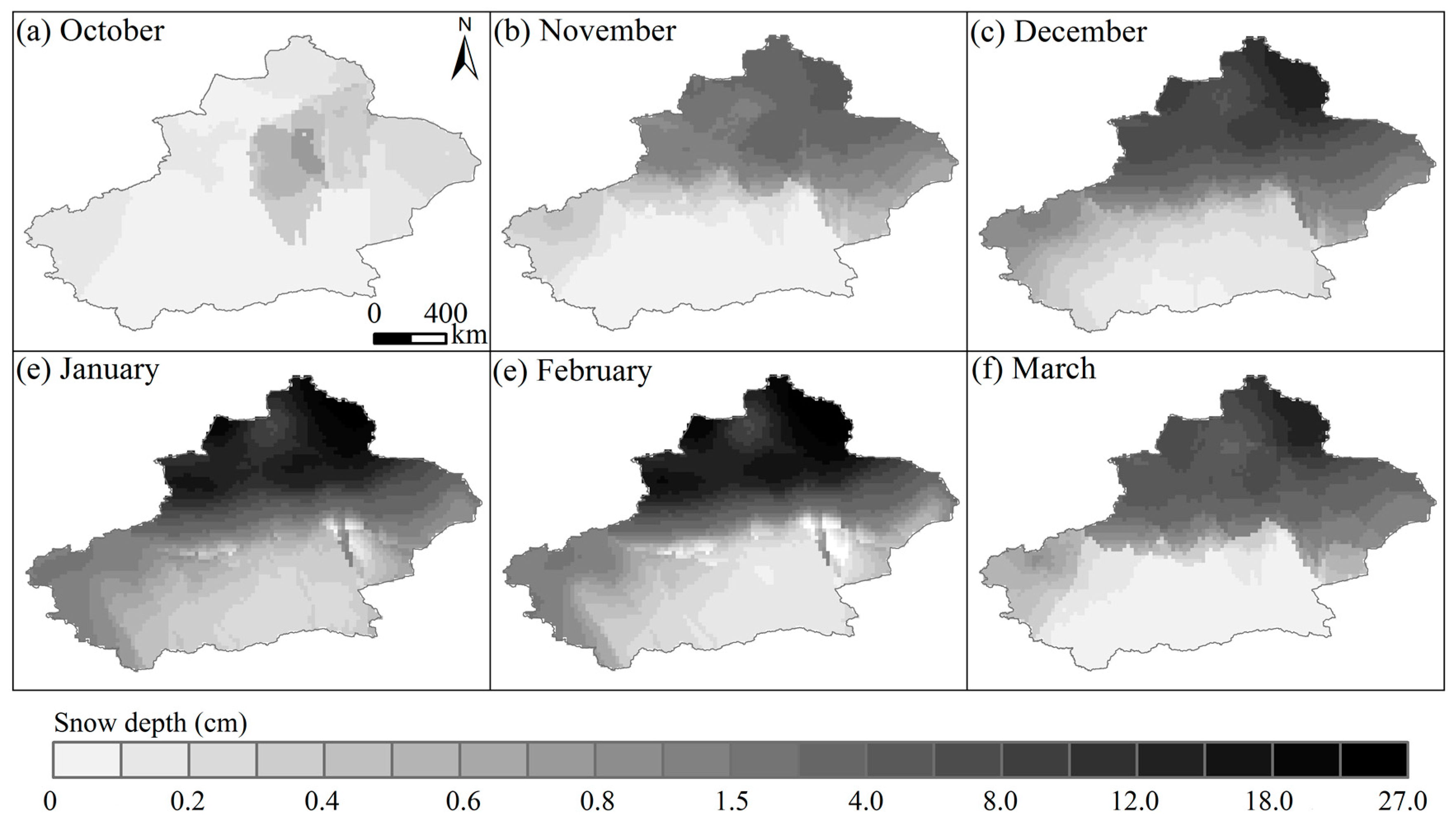
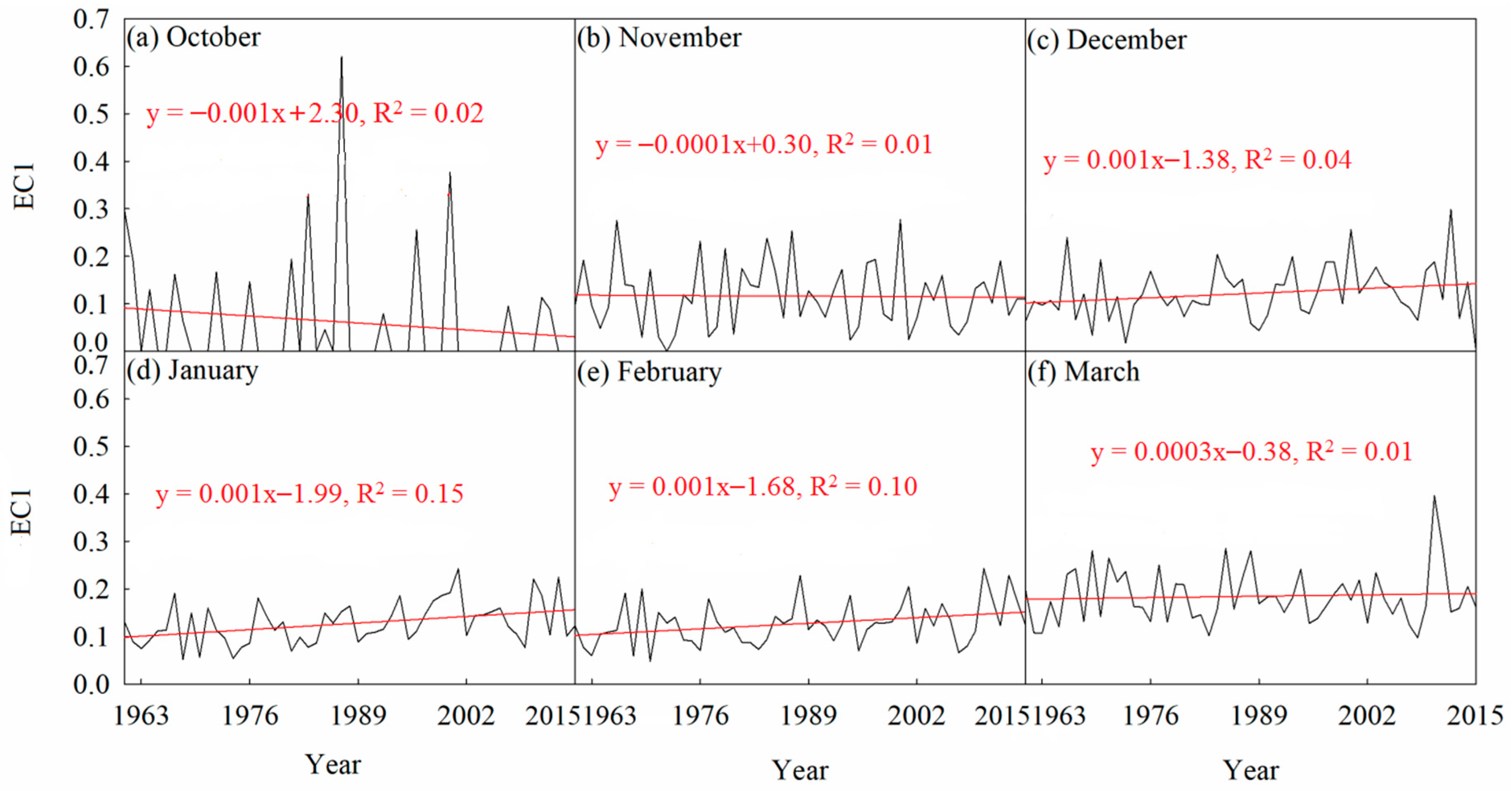
Based on the observed values, the yearly variations and spatial distribution of monthly snow depths in Xinjiang are illustrated in Figure 2 and Figure 3. The fluctuations and ranges of snow depths differed for the six months both temporally and spatially. Although almost half of the year snow is a main precipitation form, generally much smaller values were observed in October and November than in December to March. Snow depth showed weak decreasing trends with the linear slopes of −0.001 and −0.002 cm year−1 in October and November (Figure 2a,b). Through MMK, the trends of snow depth in these two months were not significant ( of October was 1.92; of November was 0.27). In the other four months the linear slopes were positive and ranged between 0.011 and 0.071 cm year−1, indicating much stronger increasing trends (Figure 2c–f). Either negative or positive, all were close to 0. Through MMK, only the trend of snow depth in January was significant ( of January was 1.96), and the trends of snow depth in other months were not significant ( of December was 1.87; of February was 1.92; of March was 0.57). From the spatial distributions, the monthly snow depths in north Xinjiang and Tianshan Mountains area had much larger values and stronger spatial differences than south Xinjiang, October was much larger in northeastern Xinjiang (near Altai mountain).
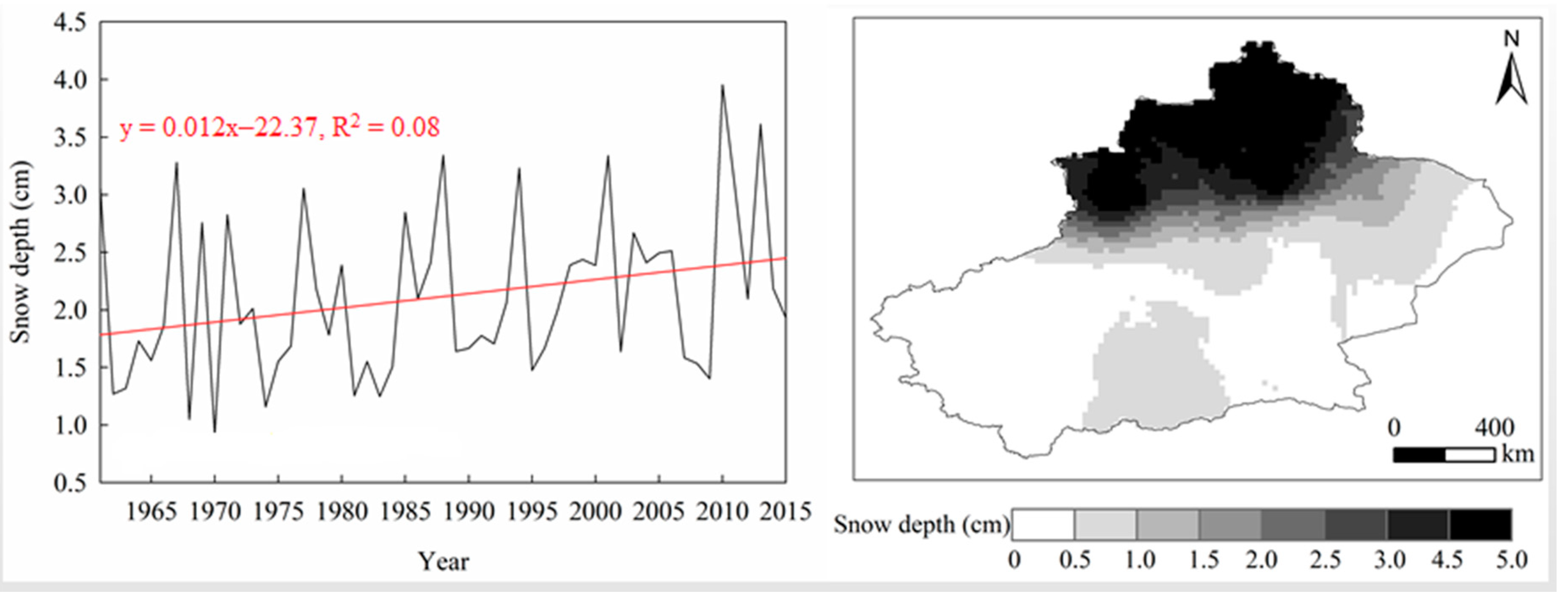
The variations of annual snow depth in Figure 4 indicated general increasing trend in Xinjiang with a linear slope of 0.012 cm year−1. Through MMK, the trend of annual snow depth was not significant ( was 1.92). The snow depth was the deepest in 2010 (3.95 cm). The spatial distribution pattern of annual snow depth was close to that of monthly values, namely, highest rates were recorded in north Xinjiang and Tianshan Mountains area than in south Xinjiang, but had much smaller ranges. Snow depth in south Xinjiang was low because south Xinjiang is warmer and drier [6].
3.2. The Decomposed Monthly and Annual Snow Depth Using EOF
EOF was used for spatiotemporally decomposing monthly or annual snow depths at each station. The decomposed EOF components varied from month to month. From explanatory weights in Table 1, taking October as an example, the variances of EOF spatial modes 1 (EOF1), 2 (EOF2), 3, (EOF3) and 4 (EOF4) explained 73.92%, 8.50%, 5.65% and 3.06% of the variability, respectively, accounting for 91.13% of the total spatial variation, of which only EOF1 was confident at the 95% level. Although EOF2 to EOF5 were insignificant, their changes explained about 10% of the total spatial variation, which meant that only on tenth of the snow depth change was random and not a temporal related spatial model. Similarly, EOF1 of snow depth in November, December, January, February and March were also a dominant component while the other EOFs accounted for minor spatial variability. EOF1, EOF2, EOF3 and EOF4 of annual snow depth explained 82.79%, 3.52%, 2.88% and 1.39% (total 90.58%) of the variability, respectively, of which only EOF1 was confident at the 95% level.
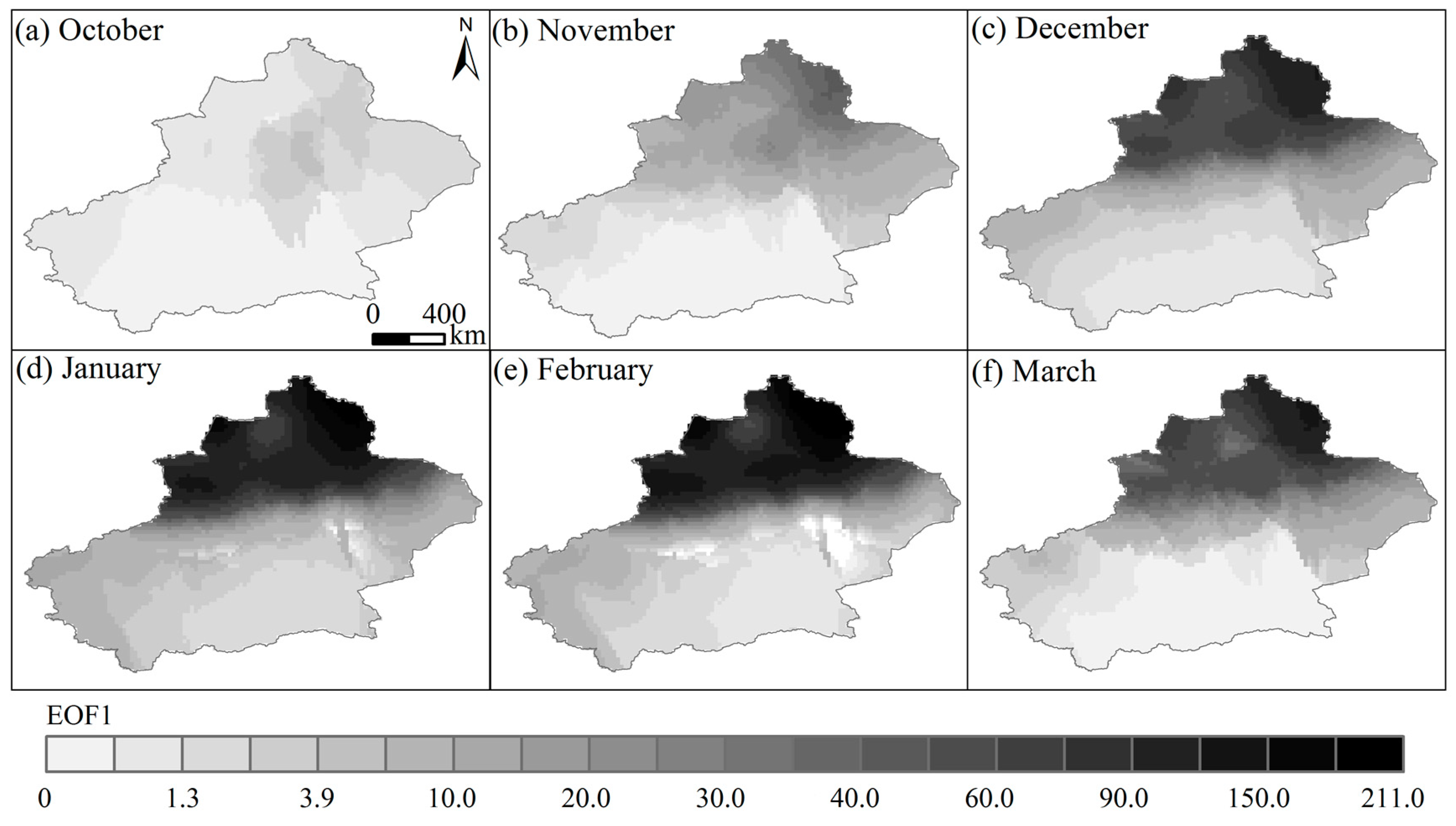
The monthly value of EOF first time mode (EC1) and monthly EOF1 which explained the dominant variability of monthly snow depth are shown in Figure 5 and Figure 6. From the EC1 curves, the linear slopes in October and November were −0.0001 and −0.001 cm year−1 (close to 0). In the other four months the slopes ranged between 0.0003 and 0.001 cm year−1 (close to 0). Through MMK, the trends of EC1 for six months were not significant ( of October was 1.86; of November was 0.43; of December was 1.83; of January was 1.80; of February was 1.95; of March was 0.42). The values of EOF1 in northern Xinjiang were much greater than south Xinjiang, indicating also greater spatiotemporal variability. The EOF1 values in five months except October were much larger in northeastern Xinjiang (near the Altai Mountain). EOF1 in October showed different change patterns in space with a small area of low values in south Xinjiang. By comparing Figure 5 and Figure 6 with Figure 2 and Figure 3 EC1 and EOF1 had much similar variations with that of the observed monthly snow depths.
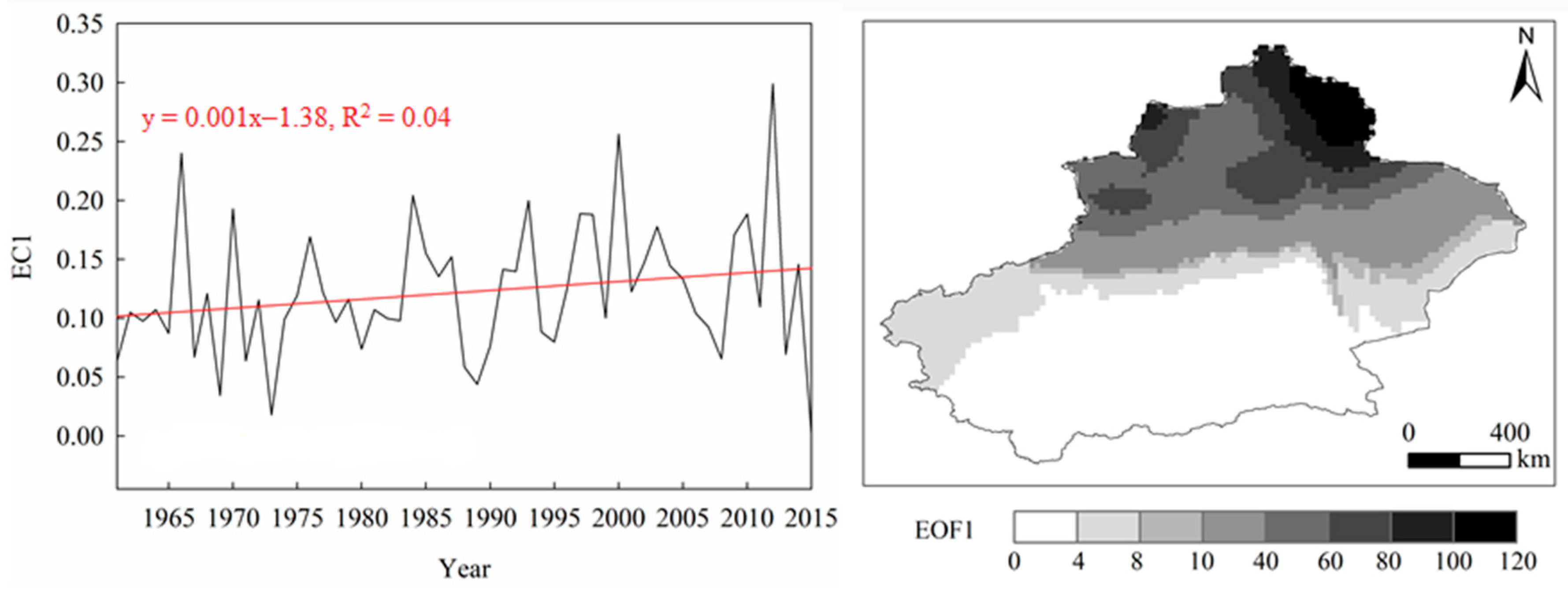
The variations of annual EC1 and EOF1 decomposed from observed annual snow depth in Xinjiang is shown in Figure 7. The linear slope was 0.001 cm year−1, indicating increasing annual EC1. Through MMK, the trend of annual EC1 was not significant ( was 1.83). The values of EOF1 in northern Xinjiang were much greater than south Xinjiang, indicating greater variability of annual snow depth. By comparing Figure 7 with Figure 4, annual EC1 had much similar variations with the observed values, while annual EOF1 generally differed with the observed values, this was reasonable because both were averaged values.
3.3. Trends and Abrupt Changes of Annual Snow Depth
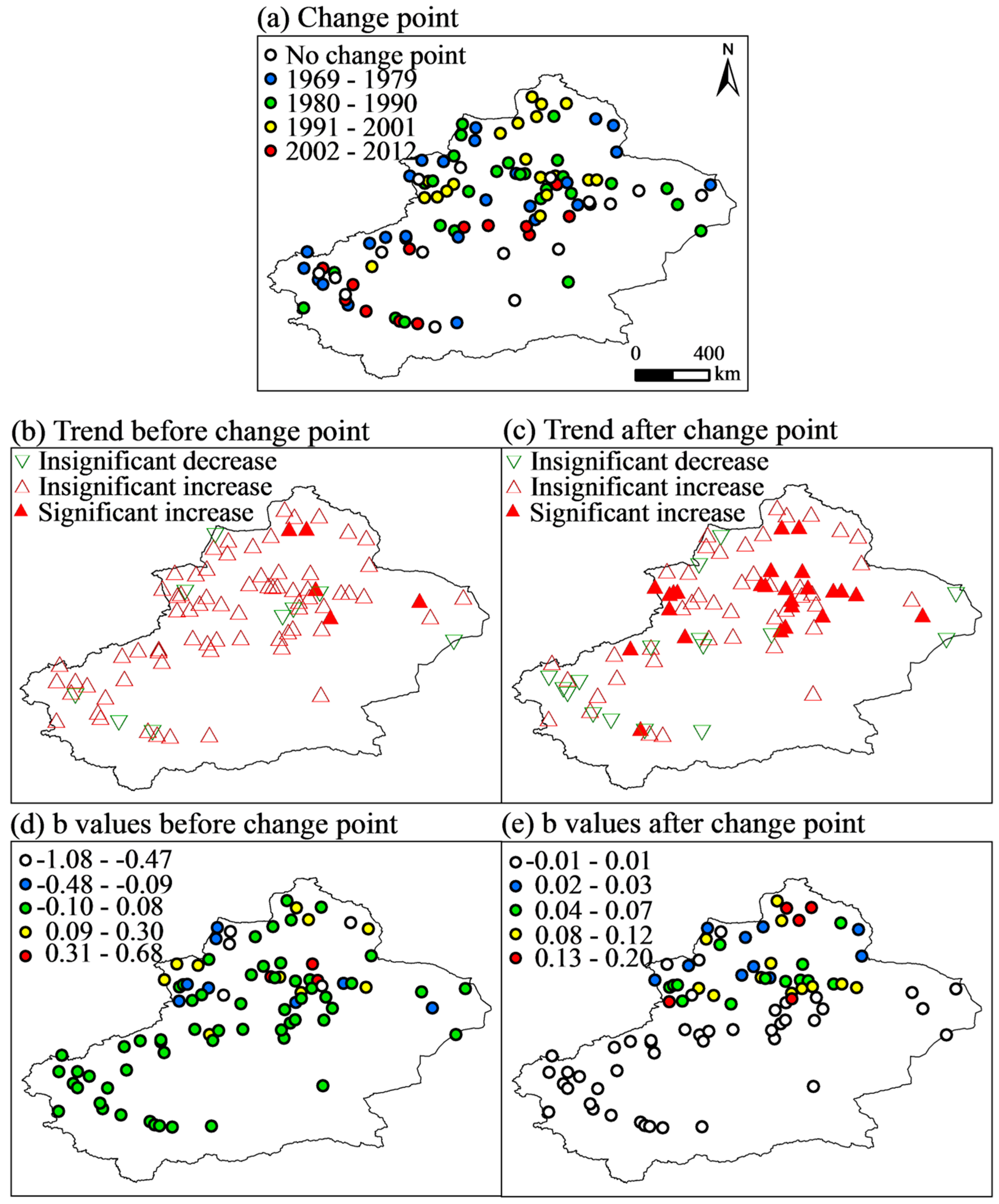
The annual snow depth had increasing trend at 64 stations, of which trends at 25 stations were significant and at 39 stations were insignificant. The annual snow depths at 85 out of 102 sites had clear abrupt changes years during 1961–2015 (tested by sequential MMK method). The year when abrupt change occurred as well as the trends before and after the change years are mapped in Figure 8. In Figure 8a, the abrupt change years mainly occurred within 1969–1979 and 1980–1990. In Figure 8b, 71 (or 9) out of 85 sites showed insignificant increasing (or insignificant decreasing) and 5 sites showed significant increasing trends before the abrupt change years. In Figure 8c, 44 (or 16) sites showed insignificant increasing (or insignificant decreasing) trends and 25 sites showed significant increasing trends after the abrupt change years. From Figure 8d, values of b (slope) before the change points varied from −1.08 to 0.68 cm year−1. From Figure 8e, values of b after the change points varied from −0.01 to 0.20 cm year−1.
3.4. Periods of Monthly and Annual Snow Depth
3.4.1. Temporal Variations
The multi-Morlet wavelet variance diagrams are used to obtain the snow depth periods at all of 102 studied sites. Taking the Aletai station (88.1° E, 47.7° N, and 736.9 m above sea level) in north Xinjiang (which is a typical site which had periodical snow depth changes, see details in Ding et al. [6]) as an example, the continuous wavelet spectrum and the periods of monthly (October, November, December, January, February and March) snow depth and annual snow depth are illustrated in Figure 9. In Figure 9a for October, from the spectrum diagram (left hand side) there was a significant main period of 5–7.5 years during 1968–1980, and two insignificant quasi-periods (2 years during 1968–1980 and 4–5 years during 1996–2000). Considering there was a certain peak in the variance diagram (right hand side) at a time scale of 6.5 years and its waveform integrity analysis, 6.5 years was determined as the main period. Similarly, in Figure 9b,c for November and December, there were significant main periods of 7 years during 1991–2007 and 6.5 years during 1984–2006. In Figure 9d for January, there were significant main periods of 7 years during 1979–1986, and an insignificant quasi-period of 6 years during 1991–1995. In Figure 9e for February, there was a significant main period of 4 years during 1996–1997, and an insignificant quasi-period of 3.5 years during 2006–2009. In Figure 9f for March, there was a significant main period of 7 years during 1978–1988, and two insignificant quasi-periods (2 years during 1966–1971 and 4 years during 2005–2010). Compared with the other five months, the main periods in February were shorter, indicating snow depths in February fluctuated more. Figure 9g shows the multi-Morlet spectrum and variance of annual snow depth at Aletai station. There was a main period of 6.5 years during 1982–1998 where the annual snow depth had strong oscillations. There was no significant quasi-period. The variance curve was generally flat except at the main-period. In general, both of the main periods and variance of annual snow depth were different compared with that of monthly snow depth.
3.4.2. Spatial Distribution
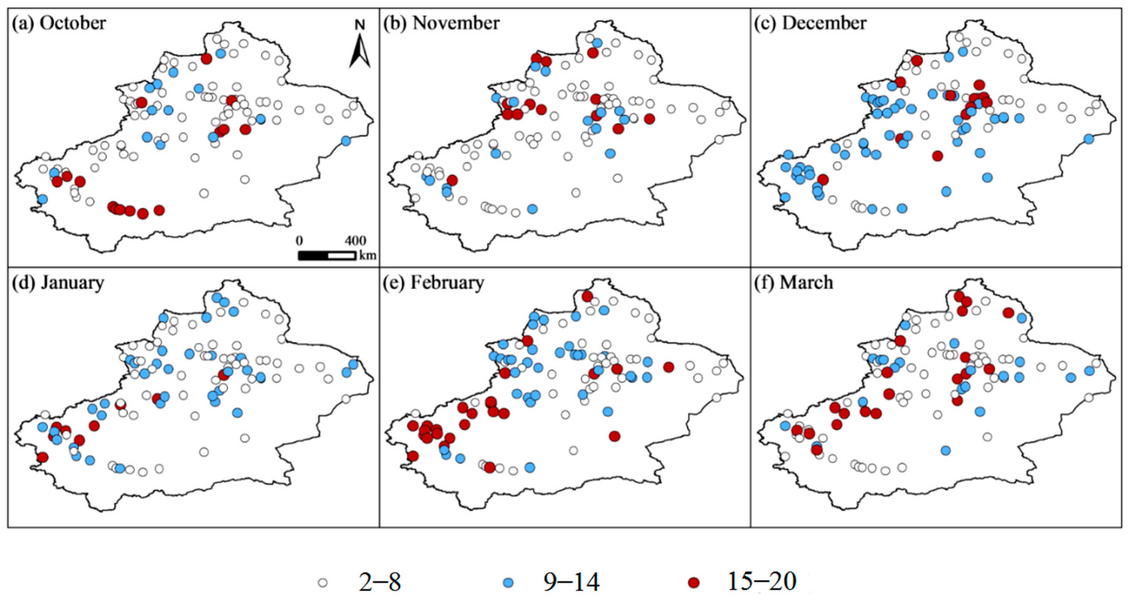
Similar to the procedures for Aletai station, periods in monthly and annual snow depths at the other 101 stations in Xinjiang over 1961–2015 were detected using the multi-Morlet wavelet analysis. The spatial distribution of main periods of the monthly snow depths (in October, November, December, January, February and March) over 1961–2015 in Xinjiang is mapped in Figure 10. Three period ranges were indicated, namely a short period of 2–8 years (white circle), medium period of 9–14 years (blue circle) and long period of 15–20 years (red circle), respectively. The short and medium periods mainly occurred in north Xinjiang, and the long periods mainly distributed in the northeastern–southwestern belt. Overall, the main periods of snow depths varied with different locations and months.
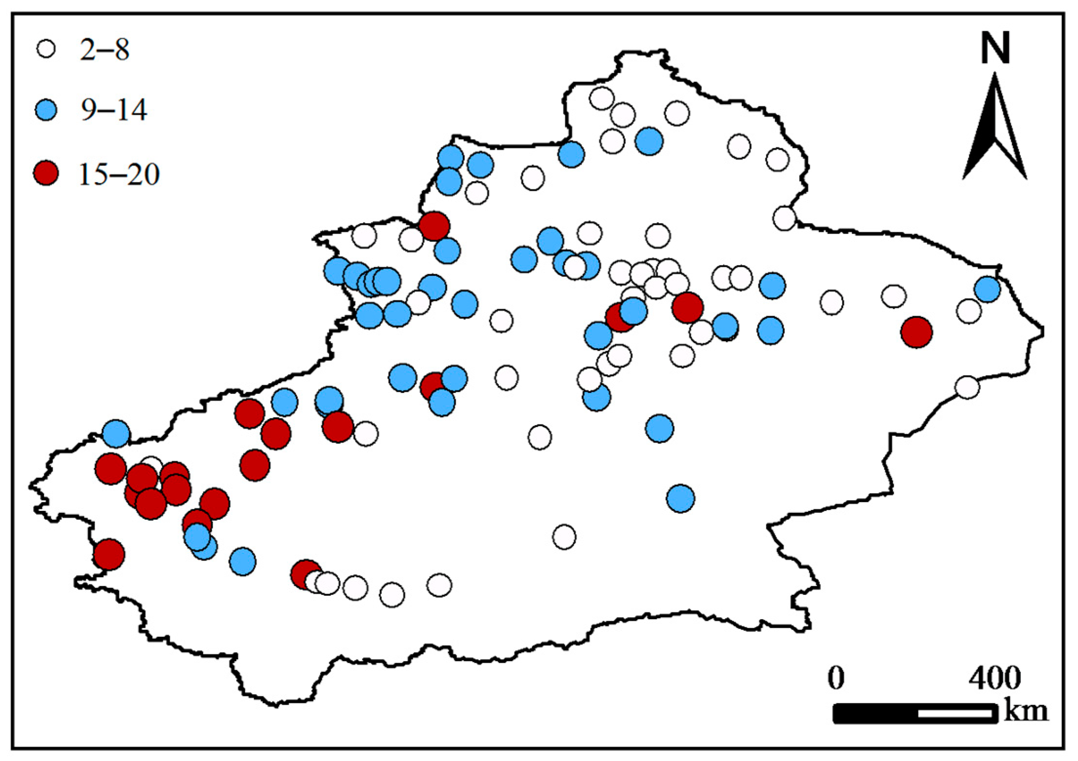
The spatial distribution of main periods of the annual snow depth in Xinjiang is mapped in Figure 11. The short and medium periods were mainly distributed in north Xinjiang, and the long period was mainly distributed in southwestern Xinjiang.
The number of the sites that had certain ranges of main period in monthly and annual snow depths in Xinjiang over 1961–2015 are presented in Table 2. As the periods increased from 2–8 to 9–14 and to 15–20 years, the number of the sites that had corresponding periods decreased, indicating common short periods in monthly and annual snow depths.
3.5. Variations of Annual Snow Depths Decomposed by Daubechies Wavelet
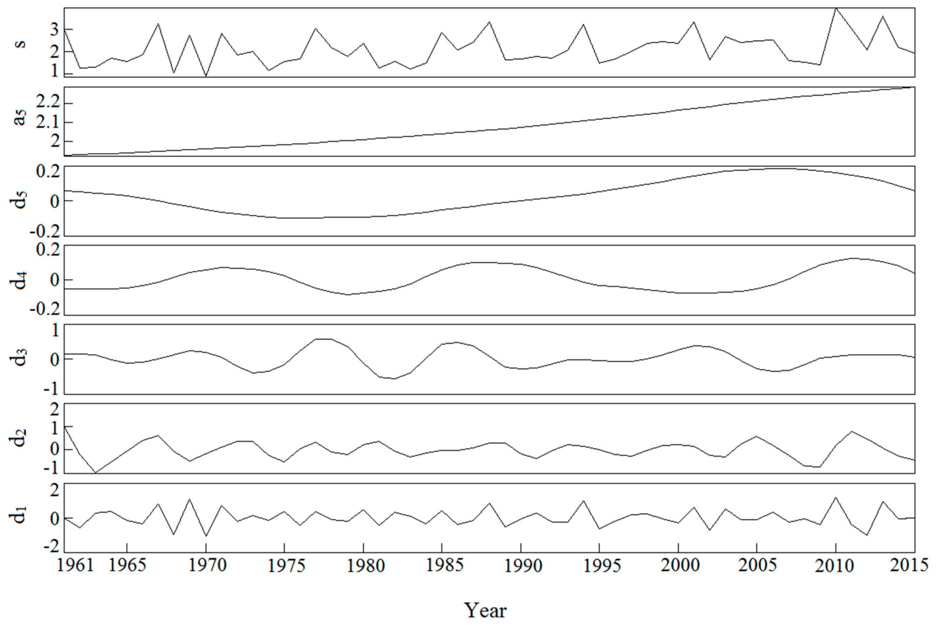
The Daubechies wavelet was applied to decompose annual snow depth series with the noise reduction processing for each site, north Xinjiang, Tianshan Mountains area, south Xinjiang and entire Xinjiang. The changes of the decomposed sub-series of annual snow depth over 1961–2015 in entire Xinjiang is illustrated in Figure 12. The annual snow depth in entire Xinjiang were decomposed to five layers of detail signals (d1 to d5) and the fifth layer of wavelet decomposition approximation signal (a5). As the decomposition gradually continued, the noise signal decayed at the high frequency signal, and the main trend in annual snow depth became more obvious. From a5 series, the annual snow depth tended to increase over 1961–2015, which agreed well with the results of EOF and MMK test.
3.6. The Coherence between Annual Snow Depth and Related Climatic Variables
The wavelet coherence relationships between annual snow depth and related climatic variables were analyzed using the cross-wavelet for entire Xinjiang (Figure 13). In Figure 13a, there was a positive correlation between annual snow depth and annual precipitation in Xinjiang, mainly concentrated in the 7–13 years’ band (during 1970–2000) and a positive correlation (phase angle of around 45°) with a 3.5–8 years’ band (2002–2009). In Figure 13b, annual snow depth was correlated positively with relative humidity with a 5.5–8 years’ band (1991–2008) and correlated positively at phase angle of 330° with a 2–3.5 years’ band (1966 to 1973). In Figure 13c, negative correlation was watched between annual snow depth and sunshine hours (at a phase angle of 225°) with a 5–10 years’ band (1970 to 2008). In Figure 13d, there was a positive correlation (around 30°) between annual snow depth and minimum temperature with a 3–4 years’ band (2008–2011) and a negative correlation (135°) with a 2.5–3.5 years’ band (1965–1971). The annual snow depth had a good correlation with precipitation, mainly because snowfall is an important part of precipitation. Weak correlation between annual snow depth and minimum temperature maybe because more weather systems bring more precipitation in the cold years, and vice versa. In general, snow depth was affected by multiple climatic variables rather than single.
4. Discussions
4.1. Spatiotemporal Variability of Snow Depths in Xinjiang
Xinjiang is a region where snow water resources are main water resources, and snow depths variations in Xinjiang in recent decades have been studied using different time-series methods including wavelet analysis. Liu et al. [9] applied wavelet analysis to investigate the periodic characteristics of maximum snow depths of 51 stations in northern Xinjiang over 1961–2008. They found that the periods in maximum snow depths were significant, and the main periods in Altay and Tacheng basin (both were located in northern Xinjiang) were 7 years and 11 years, respectively. This study found that the main periods were longer, which may be due to our longer study period (1961–2015) and larger number of sites (102). We found that the short periods (2–8 years) and medium periods (9–14 years) were mainly distributed in north Xinjiang. Mazzarella et al. [50] found that multivariate El Niño Southern Oscillation (ENSO) index had a short period of 5 years. Their result was similar to a short period of snow depth. Ding et al. [6] applied the MMK test to investigate the trends with significance and analyzed the ECs and EOFs of daily snow depths over 1961–2013 at 105 stations in Xinjiang, China. They found that the snow depths at 86 stations had growing trends. The EC1 values in entire Xinjiang had obvious yearly fluctuations without typical trends. Values of EOF1 in north Xinjiang were larger than that in south Xinjiang. This research applied the sequential MMK test and found the change points of annual snow depths and trends before and after the change points. It was reasonable that trends differed between daily Ding et al. [6] and annual time scales (this research). Further, we systematically investigated the variability of monthly and annual snow depth in Xinjiang, which had not been studied in Ding et al. [6].
4.2. The Applications of Multi-Wavelet Methods
The EOF method supplied the main spatial and temporal components that explained large parts of snow depth variability. The change points and the trend before and after the change points of the annual snow depth were tested by the modified Mann–Kendall method in this research to reveal the variation characteristics statistically. Specially, different wavelet methods, namely the multi-Morlet, Daubechies and cross wavelets were used to comprehensively reveal the periods and oscillations, fluctuations, decomposed sub-series and correlations (with climatic variables) of monthly and annual snow depths in Xinjiang from different respects. Former studies generally applied less methods. Therefore, the combination of different methods supplied comprehensively interrogate the system for investigating spatial–temporal variability of snow depths.
4.3. Impact of Various Factors on the Snow Depth and Potential Effects of Variations in Snow Depth
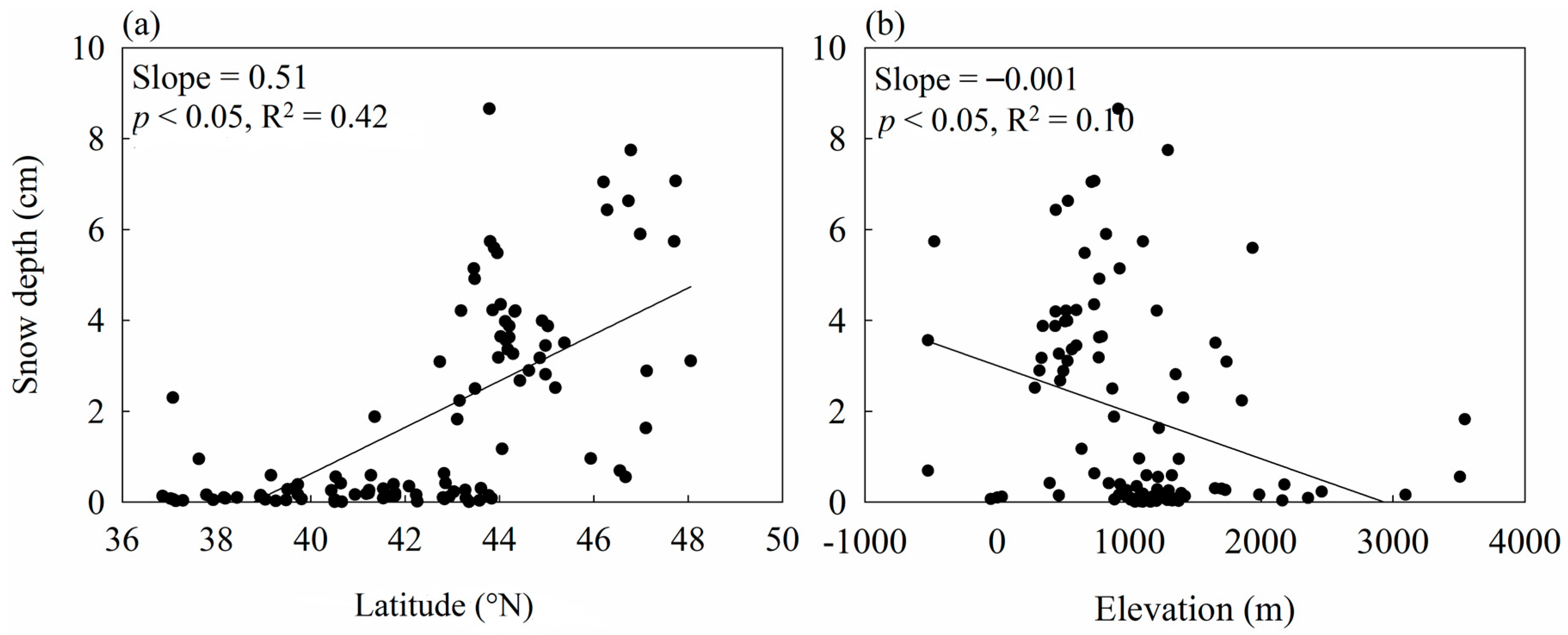
Topography is an important factor affecting climatology of snow depth and a main reason accounting for snow depth data inhomogeneity [51]. In order to reveal the influence of complex terrain on annual snow depth in Xinjiang, we conducted a linear regression analysis of annual snow depth with latitude and elevation (Figure 14). Generally, the annual snow depth increased with the increasing latitude with a slope of 0.51 cm/° (Figure 14a). North of 40° N, the annual snow depth was relatively stable (<2 m). However, the annual snow depth was correlated poorly to elevation (Figure 14b).
Besides the topographical factors, changes in snow depth were also closely related to climatic variables. As to the correlations between snow parameters and climatic variables, Xu et al. [11] used a linear model to analyze the correlations between annual mean temperature and precipitation and the snow accumulation duration in the Qinghai–Tibetan Plateau, China over 1961–2010. It was found that snow cover was controlled by multiple climate factors. The annual mean temperature was positively correlated with snow starting time, but negatively correlated with snow ending time. However, both starting and ending times were not significantly correlated with precipitation. This research applied cross wavelet to relate some key climate variables to annual snow depth, and found that the annual snow depths were correlated well with precipitation, had low negative correlation with minimum temperature, and had good positive correlation with relative humidity. Hu et al. [10] analyzed the correlations between annual snow depth and precipitation (or average temperature) in Xinjiang over 1960–2011. They found good correlations of snow depth with precipitation but low correlation with mean temperature. Their results agreed well with ours although the number of sites and study period were different. The connections between snow depth and climate variables could be further studied using the other methods such as multi-variate regression or some machine study methods. In terms of our results, the increased relative humidity implied more water supply for snowfall, which resulted in increasing snow depths. The significant increase in snow depth can explain the sudden drop in snow density from the mid-1990s to the early 2000s [52], namely an increase in snowfall reduced the density of surface snow. This suggested that extreme snow events may be the main reason of the increase in annual snow depth. There was no statistically significant correlation between annual average snow depth and temperature. This is because in cold regions where the temperature rise is still below the freezing point, the temperature has no significant effect on the annual snow depth. In addition, atmospheric circulation is also a key factor affecting the change in snow depth. These factors and associated uncertainties accounted for regional and temporal differences in snow depth changes. In response to climate change, snow cover and snow duration were reduced, however, snow depth increased significantly.
Snow depth is an important factor in controlling ground temperature [53]. Thin snow cover causes soil surface to be cold, while thick snow cover causes soil surface to be warmer. We have reached the conclusion that the snow depth in Xinjiang has risen through EOF, MMK and db5 wavelet analysis. Although the effect of snow depth on cooling or warming in Xinjiang is still unclear, the decrease in snow depth will reduce the warming effect and offset the increase in permafrost temperature. Conversely, an increase in snow depth will further increase the temperature of permafrost and enhance the degradation of permafrost in the area. Meanwhile, the snow depth also has an important impact on the hydrological cycle. Spring flooding is induced by snowmelt, the increase in snow depth in Xinjiang may lead to spring flooding in Xinjiang, especially in the north. Snow also interacts with vegetation, which affects the depth, redistribution and vertical profile of the forest or shrub. Snow depth also affects plant growth. The increase of snow depth in Xinjiang may generate more water content, which can increase soil moisture and vegetation productivity.
Fractal analysis is a good tool for analyzing snow characteristics. When snow depth was governed by different factors interconnected among themselves in a non-linear way, they obeyed fractal (power-law) statistics. Although it was not taken into account in this research, it has been used to model snow crystals and geometrical topography of snowflakes [54]. The complexity of such phenomena do not depend on the number of causes that govern it but essentially on the number of their interconnections, on the magnitude of such linkages and on the feedback processes. In these cases, the whole system is more than the sum of its parts and its response to an external forcing does not follow a linear but a power-law relationship.
It should be noted that the current analysis is based on station observations. It is still insufficient to fully characterize snow depth variability in Xinjiang. Satellite-based snow products provide big data sets at different spatial–temporal scales in unobserved areas. In future research station-observed data could be integrated with satellite observations to investigate snow changes at large spatial scales in Xinjiang.
5. Conclusions
The spatiotemporal variability of monthly and annual snow depths was systematically investigated for Xinjiang using several time-series analysis methods, namely EOF, sequential MMK, multi-Morlet wavelet, Daubechies wavelet, and cross wavelet. The EOF-decomposed EC1 curves of snow depths had decreased trends in October and November, and increased in the other four months. For all the six months, the values of EOF1 in northern Xinjiang were much greater than south Xinjiang, indicating greater variability. The annual EC1 curve had increasing linear slope of 0.0008. Both the variation patterns of monthly and annual EC1 curves agreed well with the observed snow depths. Similarly, the monthly and annual EOF1 in northern Xinjiang were greater than southern Xinjiang. The spatial distribution of monthly EOF1 had similar pattern with the observed annual snow depths.
From the sequential MMK test, the abrupt-change points mainly occurred during 1969–1979 and 1980–1990. The annual snow depth of most sites showed increasing trends, but with different slope magnitudes.
From the multi-Morlet wavelet, monthly and annual snow depths generally had main periods of 2–20 years. The sites that had main periods of 2–8 and 9–14 years (15–20 years) in monthly and annual snow depths mainly distributed in northern (southwestern) Xinjiang. From the Daubechies wavelet decomposition results, the annual snow depth tended to increase in entire Xinjiang, which agreed well with the results of the EOF and MMK test. The cross wavelet-transform showed good correlations between annual snow depth and precipitation (or relative humidity), but poor correlations with minimum temperature (or sunshine hours). Overall, the combination of different methods supplied comprehensive interrogation for investigating spatial–temporal variability of snow depths. Further research would be applied for larger spatial scale based on remote-sensing data.
Author Contributions
All authors listed have contributed to this study. Conceptualization, Y.L. (Yi Liu), Y.L. (Yi Li), L.L. and C.C.; Methodology, Y.L. (Yi Liu), Y.L. (Yi Li) and L.L.; Formal Analysis, Y.L. (Yi Liu) and L.L.; software, Y.L. (Yi Liu) and L.L.; validation, Y.L. (Yi Liu).and L.L.; Writing—Original Draft Preparation, Y.L. (Yi Liu) and Y.L. (Yi Li); Writing—Review & Editing, Y.L. (Yi Liu) and Y.L. (Yi Li).
Funding
The authors acknowledge the National Key Research and Development Program of China (No. 2017YFC0403303), the High-End Foreign Experts Introduction Project, and the “111 Project” of China (No. B12007) for granting support.
Acknowledgments
The authors sincerely thank the researchers and staff members for their help and thank editors and reviewers for reviewing the manuscript.
Conflicts of Interest
The authors declare no conflict of interest.
Abbreviations
| EOF | Empirical orthogonal function |
| EOF1 | EOF first spatial mode |
| DBN | Daubechies wavelet |
| MMK | Modified Mann–Kendall |
| EC1 | EOF first time mode |
References
- Wang, J.; Wang, L. A review on snow cover and snowmelt runoff simulation using remote sensing data sets in China. Proc. SPIE Int. Soc. Opt. Eng. 2003, 4894, 446–455. [Google Scholar] [CrossRef]
- Yang, Z.L.; Dickinson, R.E.; Robock, A.; Vinnikov, K.Y. Validation of the Snow Submodel of the Biosphere–Atmosphere Transfer Scheme with Russian Snow Cover and Meteorological Observational Data. J. Clim. 1997, 10, 353–373. [Google Scholar] [CrossRef]
- Dey, B.; Kumar, O.S.R.U.B. Himalayan winter snow cover area and summer monsoon rainfall over India. J. Geophys. Res. Ocean. 1983, 88, 5471–5474. [Google Scholar] [CrossRef]
- Hahn, D.G.; Shukla, J. An Apparent Relationship between Eurasian Snow Cover and Indian Monsoon Rainfall. J. Atmos. Sci. 1976, 33, 2461–2462. [Google Scholar] [CrossRef] [Green Version]
- Lamb, H.H. Two-way relationship between the snow or ice limit and 1,000– 500 mb thicknesses in the overlying atmosphere. Q. J. R. Meteorol. Soc. 2010, 81, 496–498. [Google Scholar] [CrossRef]
- Ding, Y.; Li, Y.; Li, L.; Yao, N.; Hu, W.; Yang, D.; Chen, C. Spatiotemporal variations of snow characteristics in Xinjiang, China over 1961–2013. Hydrol. Res. 2018, 49, 1578–1593. [Google Scholar] [CrossRef]
- Brun, E.; Vionnet, V.; Boone, A.; Decharme, B.; Peings, Y.; Valette, R.; Karbou, F.; Morin, S. Simulation of Northern Eurasian Local Snow Depth, Mass, and Density Using a Detailed Snowpack Model and Meteorological Reanalyses. J. Hydrometeorol. 2013, 14, 203–219. [Google Scholar] [CrossRef]
- Kern, S.; Ozsoy-Çiçek, B. Satellite Remote Sensing of Snow Depth on Antarctic Sea Ice: An Inter-Comparison of Two Empirical Approaches. Remote Sens. 2016, 8, 450. [Google Scholar] [CrossRef]
- Liu, Y.; Ruan, H.; Zhang, Y.; Li, Y. Spatio-Temporal Characteristics of the Snow Cover Ecllution in the Northern Region of Xinjiang over the Period of 1961—2008. Resour. Sci. 2012, 34, 629–635. [Google Scholar] [CrossRef]
- Hu, L.; Li, S.; Liang, F. Analysis of the variation characteristics of snow covers in Xinjiang region during recent 50 years. J. Glaciol. Geocryol. 2013, 35, 793–800. [Google Scholar] [CrossRef]
- Xu, W.; Ma, L.; Ma, M.; Zhang, H.; Yuan, W. Spatial-temporal variability of snow cover and depth in Qinghai-Tibetan Plateau. J. Clim. 2015, 30, 1522–1533. [Google Scholar] [CrossRef]
- Che, T.; Li, X.; Jin, R.; Armstrong, R.; Zhang, T. Snow depth derived from passive microwave remote-sensing data in China. Ann. Glaciol. 2008, 49, 145–154. [Google Scholar] [CrossRef] [Green Version]
- Huang, N.E.; Shen, Z.; Long, S.R.; Wu, M.C.; Shih, H.H.; Zheng, Q.; Yen, N.C.; Tung, C.C.; Liu, H.H. The empirical mode decomposition and the Hilbert spectrum for nonlinear and non-stationary time series analysis. Proc. Math. Phys. Eng. Sci. 1998, 454, 903–995. [Google Scholar] [CrossRef]
- Nourani, V.; Alami, M.T.; Aminfar, M.H.; Aalami, M.T. A combined neural-wavelet model for prediction of Ligvanchai watershed precipitation. Eng. Appl. Artif. Intell. 2009, 22, 466–472. [Google Scholar] [CrossRef]
- Cortes, C.; Vapnik, V. Support-Vector Networks. Mach. Learn. 1995, 20, 273–297. [Google Scholar] [CrossRef]
- Priestley, M.B. Spectral Analysis and Time Series; Academic Press: Cambridge, MA, USA, 1981; pp. 179–183. [Google Scholar]
- Grossmann, A.; Kronland-Martinet, R.; Morlet, J. Reading and Understanding Continuous Wavelet Transforms. Wavelets 1990, 31, 2–20. [Google Scholar] [CrossRef]
- Lorenz, E.N. Empirical Orthogonal Functions and Statistical Weather Prediction; Massachusetts Institute of Technology, Dept. of Meteorology: Cambridge, MA, USA, 1956. [Google Scholar]
- Hu, W.; Si, B.C. Estimating spatially distributed soil water content at small watershed scales based on decomposition of temporal anomaly and time stability analysis. Hydrol. Earth Syst. Sci. 2016, 20, 571–587. [Google Scholar] [CrossRef] [Green Version]
- Kim, S.E.; Seo, I.W.; Choi, S.Y. Assessment of water quality variation of a monitoring network using exploratory factor analysis and empirical orthogonal function. Environ. Model. Softw. 2017, 94, 21–35. [Google Scholar] [CrossRef]
- Yang, P.; Xia, J.; Zhan, C.; Qiao, Y.; Wang, Y. Monitoring the spatio-temporal changes of terrestrial water storage using GRACE data in the Tarim River basin between 2002 and 2015. Sci. Total Environ. 2017, 595, 218–228. [Google Scholar] [CrossRef]
- Achuthavarier, D.; Schubert, S.D.; Vikhliaev, Y.V. North Pacific decadal variability: Insights from a biennial ENSO environment. Clim. Dyn. 2016, 49, 1379–1397. [Google Scholar] [CrossRef]
- Cerrone, D.; Fusco, G.; Cotroneo, Y.; Simmonds, I.; Budillon, G. The Antarctic Circumpolar Wave: Its Presence and Interdecadal Changes during the Last 142 Years. J. Clim. 2017, 30, 6371–6389. [Google Scholar] [CrossRef]
- Sang, Y.F.; Wang, D.; Wu, J.C.; Zhu, Q.P.; Wang, L. Entropy-Based Wavelet De-noising Method for Time Series Analysis. Entropy 2009, 11, 1123–1147. [Google Scholar] [CrossRef] [Green Version]
- Whitcher, B.; Byers, S.D.; Guttorp, P.; Percival, D.B. Testing for homogeneity of variance in time series: Long memory, wavelets, and the Nile River. Water Resour. Res. 2002, 38. [Google Scholar] [CrossRef]
- Torrence, C.; Compo, G.P. A Practical Guide to Wavelet Analysis. Bull. Am. Meteorol. Soc. 1998, 79, 61–78. [Google Scholar] [CrossRef] [Green Version]
- Labat, D. Recent advances in wavelet analyses: Part 1. A review of concepts. J. Hydrol. 2008, 314, 275–288. [Google Scholar] [CrossRef]
- Schaefli, B.; Maraun, D.; Holschneider, M. What drives high flow events in the Swiss Alps? Recent developments in wavelet spectral analysis and their application to hydrology. Adv. Water Resour. 2007, 30, 2511–2525. [Google Scholar] [CrossRef] [Green Version]
- Rashid, M.M.; Beecham, S.; Chowdhury, R.K. Assessment of trends in point rainfall using Continuous Wavelet Transforms. Adv. Water Resour. 2015, 82, 1–15. [Google Scholar] [CrossRef]
- Kuang, C.P.; Su, P.; Gu, J.; Chen, W.J.; Zhang, J.L.; Zhang, W.L.; Zhang, Y.F. Multi-time scale analysis of runoff at the Yangtze estuary based on the Morlet Wavelet Transform method. J. Mt. Sci. 2014, 11, 1499–1506. [Google Scholar] [CrossRef]
- Li, Y.; Sun, C. Impacts of the superimposed climate trends on droughts over 1961–2013 in Xinjiang, China. Theor. Appl. Climatol. 2017, 129, 1–18. [Google Scholar] [CrossRef]
- Li, Y.; Yao, N.; Sahin, S.; Appels, W.M. Spatiotemporal variability of four precipitation-based drought indices in Xinjiang, China. Theor. Appl. Climatol. 2017, 129, 1017–1034. [Google Scholar] [CrossRef]
- Zhang, Q.; Singh, V.P.; Li, J.; Jiang, F.; Bai, Y. Spatio-temporal variations of precipitation extremes in Xinjiang, China. J. Hydrol. 2012, 434, 7–18. [Google Scholar] [CrossRef]
- Guo, C.; Li, B.; Yang, S.; Zhuang, X.; Wang, H. Analysis of Climate Characteristic of Heavy Snowstorm in Altay Region of Xinjiang. J. Arid Meteorol. 2012, 30, 604–608. [Google Scholar]
- Hirsch, R.M.; Helsel, D.R.; Cohn, T.A.; Gilroy, E.J.; Maidment, D.R. Statistical analysis of hydrologic data. Mod. Diagn. Treat. 1992, 17, 1–17. [Google Scholar]
- Yue, S.; Wang, C. The influence of serial correlation on the Mann–Whitney test for detecting a shift in median. Adv. Water Resour. 2002, 25, 325–333. [Google Scholar] [CrossRef]
- Perry, M.A.; Niemann, J.D. Analysis and estimation of soil moisture at the catchment scale using EOFs. J. Hydrol. 2007, 334, 388–404. [Google Scholar] [CrossRef]
- Sun, Z.; Opp, C. Characterizing snow cover interannual variability with Empirical Orthogonal Function (EOF) analysis and its climate effect in the inland region, Northwest China. MIPPR 2009 Remote Sens. GIS Data Process. Other Appl. 2009, 7498. [Google Scholar] [CrossRef]
- .Yue, S.; Wang, C.Y. Regional streamflow trend detection with consideration of both temporal and spatial correlation. Int. J. Clim. 2002, 22, 933–946. [Google Scholar] [CrossRef]
- Kendall, M. Rank Correlation Methods; Charles, G., Ed.; Google Scholar: London, UK, 1975. [Google Scholar]
- Mann, H. Nonparametric tests against trend. Econometrica 13 245259Milly PCD, Dunne KA (2002) Macro scale water fluxes 2, water and energy supply control of their enter-annual variability. Water Resour. Res. 1945, 38, 241249. [Google Scholar]
- Li, Y.; Horton, R.; Ren, T.; Chen, C. Prediction of annual reference evapotranspiration using climatic data. Agric. Water Manag. 2010, 97, 300–308. [Google Scholar] [CrossRef]
- Li, Y.; Yao, N.; Chau, H.W. Influences of removing linear and nonlinear trends from climatic variables on temporal variations of annual reference crop evapotranspiration in Xinjiang, China. Sci. Total Environ. 2017, 592, 680–692. [Google Scholar] [CrossRef] [Green Version]
- Partal, T.; Kahya, E. Trend analysis in Turkish precipitation data. Hydrol. Process. 2006, 20, 2011–2026. [Google Scholar] [CrossRef]
- Whitcher, B.; Guttorp, P.; Percival, D.B. Wavelet analysis of covariance with application to atmospheric time series. J. Geophys. Res. Atmos. 2000, 105, 14941–14962. [Google Scholar] [CrossRef] [Green Version]
- Foufoula-Georgiou, E.; Kumar, P. Wavelet analysis for geophysical applications. Rev. Geophys. 1997, 35, 385–412. [Google Scholar] [CrossRef] [Green Version]
- Lina, J.M. Complex Daubechies Wavelets: Filters Design and Applications. In Inverse Problems Tomography Image Processing; Springer: Boston, MA, USA, 1997; pp. 1–18. [Google Scholar]
- Torrence, C.; Webster, P.J. Interdecadal Changes in the ENSO–Monsoon System. J. Clim. 1999, 12, 2679–2690. [Google Scholar] [CrossRef]
- Maraun, D.; Kurths, J. Cross wavelet analysis: Significance testing and pitfalls. Nonlinear Process. Geophys. 2004, 11, 505–514. [Google Scholar] [CrossRef]
- Mazzarella, A.; Giuliacci, A.; Liritzis, I. On the 60-month cycle of Multivariate ENSO Index. Theor. Appl. Climatol. 2010, 100, 23–27. [Google Scholar] [CrossRef]
- Grünewald, T.; Bühler, Y.; Lehning, M. Elevation dependency of mountain snow depth. Cryosphere 2014, 8, 2381–2394. [Google Scholar] [CrossRef] [Green Version]
- Zhong, X.; Zhang, T.; Wang, K. Snow density climatology across the former USSR. Cryosphere 2014, 8, 785–799. [Google Scholar] [CrossRef] [Green Version]
- Goodrich, L.E. The influence of snow cover on the ground thermal regime. Can. Geotech. J. 1982, 19, 421–432. [Google Scholar] [CrossRef] [Green Version]
- Carbone, A.; Chiaia, B.M.; Frigo, B.; Türk, C. Fractal Model for Snow. Mater. Sci. Forum 2010, 638, 2555–2560. [Google Scholar] [CrossRef]
Figure 1.
The geographical location and elevations (unit: m) of the selected 102 weather stations in Xinjiang, China. The black lines show the borders of north Xinjiang, Tianshan Mountains Area and south Xinjiang. The white dots represent the weather stations.
Figure 1.
The geographical location and elevations (unit: m) of the selected 102 weather stations in Xinjiang, China. The black lines show the borders of north Xinjiang, Tianshan Mountains Area and south Xinjiang. The white dots represent the weather stations.

Figure 2.
Temporal variation of monthly snow depth (cm) over 1961–2015 in Xinjiang: (a) October, (b) November, (c) December, (d) January, (e) February and (f) March.
Figure 2.
Temporal variation of monthly snow depth (cm) over 1961–2015 in Xinjiang: (a) October, (b) November, (c) December, (d) January, (e) February and (f) March.

Figure 3.
Spatial variation of monthly snow depth (cm) over 1961–2015 in Xinjiang: (a) October, (b) November, (c) December, (d) January, (e) February and (f) March.
Figure 3.
Spatial variation of monthly snow depth (cm) over 1961–2015 in Xinjiang: (a) October, (b) November, (c) December, (d) January, (e) February and (f) March.

Figure 4.
The temporal variations of annual snow depths (cm) over 1961–2015 and spatial distribution of long-term mean values in Xinjiang.
Figure 4.
The temporal variations of annual snow depths (cm) over 1961–2015 and spatial distribution of long-term mean values in Xinjiang.

Figure 5.
The variations of monthly EOF first time mode (EC1) in Xinjiang: (a) October, (b) November, (c) December, (d) January, (e) February and (f) March.
Figure 5.
The variations of monthly EOF first time mode (EC1) in Xinjiang: (a) October, (b) November, (c) December, (d) January, (e) February and (f) March.

Figure 6.
The variations of monthly long-term mean EOF first spatial mode (EOF1) in Xinjiang: (a) October, (b) November, (c) December, (d) January, (e) February and (f) March.
Figure 6.
The variations of monthly long-term mean EOF first spatial mode (EOF1) in Xinjiang: (a) October, (b) November, (c) December, (d) January, (e) February and (f) March.

Figure 7.
The annual EC1 and long-term mean EOF1 in Xinjiang.

Figure 8.
The spatial distribution of the change points, trends and magnitude (b values) before and after the change points: (a) Change point, (b) Trend before change point, (c) Trend after change point, (d) b values before change point and (e) b values after change point.
Figure 8.
The spatial distribution of the change points, trends and magnitude (b values) before and after the change points: (a) Change point, (b) Trend before change point, (c) Trend after change point, (d) b values before change point and (e) b values after change point.

Figure 9.
Multi-Morlet wavelet spectrum of monthly and annual snow depths over 1961–2015 at the Aletai station: (a) October, (b) November, (c) December, (d) January, (e) February (f) March and (g) Annual.The red and blue colors indicate the peak and valley of the energy density, and the color depth indicates the relative change of the energy density. The black thick solid line is the 95% confidence interval boundary and passes the red noise test. The cone of influence (COI) where edge effects may distort the picture is shown under a thin black curve.

Figure 10.
The spatial distribution of main periods in monthly snow depth in Xinjiang over 1961–2015: (a) October, (b) November, (c) December, (d) January, (e) February and (f) March.
Figure 10.
The spatial distribution of main periods in monthly snow depth in Xinjiang over 1961–2015: (a) October, (b) November, (c) December, (d) January, (e) February and (f) March.

Figure 11.
The periods spatial distribution of annual snow depth at 102 weather stations in Xinjiang over 1961–2015.
Figure 11.
The periods spatial distribution of annual snow depth at 102 weather stations in Xinjiang over 1961–2015.

Figure 12.
The decomposed Daubechies series of annual snow depth over 1961–2015 in entire Xinjiang. S represents the original signal, d1–d5 are the five layers of wavelet decomposed signal, and a5 represents the 5th layer wavelet decomposed approximation signal.
Figure 12.
The decomposed Daubechies series of annual snow depth over 1961–2015 in entire Xinjiang. S represents the original signal, d1–d5 are the five layers of wavelet decomposed signal, and a5 represents the 5th layer wavelet decomposed approximation signal.

Figure 13.
The wavelet coherence spectra between annual snow depth and (a) annual precipitation, (b) relative humidity, (c) sunshine hours and (d) minimum temperature over 1961–2015 in Xinjiang. The arrows indicate the phase relationship, the arrows pointing to the right and left indicate in-phase and inversion, while the vertical downward and vertical upwards indicate that the wavelet transform of the annual snow depth is ahead and behind one quarter period of each climate variable. Black outlines indicate areas significant at the 95% confidence level.

Figure 14.
Relationship between annual snow depth (cm) and latitude (a), elevation (b) for all stations over 1961–2015 in Xinjiang.
Figure 14.
Relationship between annual snow depth (cm) and latitude (a), elevation (b) for all stations over 1961–2015 in Xinjiang.


Table 1.
The explanatory weights of the major empirical orthogonal functions (EOFs) for monthly and annual snow depths in % (means proportion of total variance that can be explained by the corresponding EOF).
Table 1.
The explanatory weights of the major empirical orthogonal functions (EOFs) for monthly and annual snow depths in % (means proportion of total variance that can be explained by the corresponding EOF).
| EOF | October | November | December | January | February | March | Annual |
|---|---|---|---|---|---|---|---|
| EOF1 | 73.92 | 69.91 | 82.79 | 88.24 | 87.23 | 77.35 | 82.79 |
| EOF2 | 8.50 | 5.92 | 3.52 | 2.62 | 3.09 | 5.72 | 3.52 |
| EOF3 | 5.65 | 0 | 2.88 | 1.59 | 2.04 | 3.93 | 2.88 |
| EOF4 | 3.06 | 0 | 1.39 | 0.95 | 1.28 | 2.32 | 1.39 |
Table 2.
The number of sites that had different main-periods for the monthly and annual snow depths over 1961–2015 in Xinjiang.
Table 2.
The number of sites that had different main-periods for the monthly and annual snow depths over 1961–2015 in Xinjiang.
| Time Stage | Main Period (Years) | ||
|---|---|---|---|
| 2–8 | 9–14 | 15–20 | |
| October | 73 | 14 | 15 |
| November | 72 | 17 | 13 |
| December | 38 | 52 | 12 |
| January | 58 | 35 | 9 |
| February | 42 | 35 | 25 |
| March | 61 | 21 | 20 |
| Annual | 45 | 38 | 19 |
© 2019 by the authors. Licensee MDPI, Basel, Switzerland. This article is an open access article distributed under the terms and conditions of the Creative Commons Attribution (CC BY) license (http://creativecommons.org/licenses/by/4.0/).
Share and Cite
MDPI and ACS Style
Liu, Y.; Li, Y.; Li, L.; Chen, C. Spatiotemporal Variability of Monthly and Annual Snow Depths in Xinjiang, China over 1961–2015 and the Potential Effects. Water 2019, 11, 1666. https://doi.org/10.3390/w11081666
AMA Style
Liu Y, Li Y, Li L, Chen C. Spatiotemporal Variability of Monthly and Annual Snow Depths in Xinjiang, China over 1961–2015 and the Potential Effects. Water. 2019; 11(8):1666. https://doi.org/10.3390/w11081666
Chicago/Turabian StyleLiu, Yi, Yi Li, Linchao Li, and Chunyan Chen. 2019. "Spatiotemporal Variability of Monthly and Annual Snow Depths in Xinjiang, China over 1961–2015 and the Potential Effects" Water 11, no. 8: 1666. https://doi.org/10.3390/w11081666
Note that from the first issue of 2016, this journal uses article numbers instead of page numbers. See further details here.