Potential Changes in Runoff of California’s Major Water Supply Watersheds in the 21st Century

Abstract

This study assesses potential changes in runoff of California’s eight major Central Valley water supply watersheds in the 21st century. The study employs the latest operative climate projections from 10 general circulation models (GCMs) of the Coupled Model Intercomparison Project Phase 5 (CMIP5) under two emission scenarios (RCP 4.5 and RCP 8.5) to drive a hydrologic model (VIC) in generating runoff projections through 2099. Changes in peak runoff, peak timing, seasonal (major water supply season April–July) runoff, and annual runoff during two future periods, mid-century and late-century, relative to a historical baseline period are examined. Trends in seasonal and annual runoff projections are also investigated. The results indicate that watershed characteristics impact runoff responses to climate change. Specifically, for rain-dominated watersheds, runoff is generally projected to peak earlier with higher peak volumes on average. For snow-dominated watersheds, however, runoff is largely projected to peak within the same month as historical runoff has, with little changes in peak volume during mid-century but pronounced decreases during late-century under the higher emission scenario. The study also identifies changes that are common to all study watersheds. Specifically, the temporal distribution of annual runoff is projected to change in terms of shifting more volume to the wet season, though there is no significant changing trend in the total annual runoff. Additionally, the snowmelt portion of the total annual runoff (represented by April–July runoff divided by total annual runoff) is projected to decline consistently under both emission scenarios, indicative of a shrinking snowpack across the study watersheds. Collectively, these changes imply higher flood risk and lower water supply reliability in the future that are expected to pose stress to California’s water system. Those findings can inform water management adaptation practices (e.g., watershed restoration, re-operation of the current water system, investing in additional water storage) to cope with the stress.

1. Introduction

Understanding potential changes and trends in future hydro-climatic variables including runoff is important for long-term water resources planning and management [1]. Specifically, from a scientific perspective, this understanding illustrates where and when hydrologic change manifests itself as a result of a changing climate. From an operational perspective, it can guide the improvement of the existing predictive tools (e.g., water supply forecasting tool) and development of new ones to better predict future hydro-climatic events. In addition, this understanding can inform the development of adaptation and mitigation plans (e.g., drought response and recovery plans) to cope with undesirable but unavoidable future changes. This understanding is particularly crucial in semi-arid areas including the state of California. As the fifth-largest economy in the world and the home to over 39 million people [2], California faces a range of water-related challenges.

Firstly, the water supply and demand are unevenly distributed spatially and temporally. A majority of the demand, highest during the dry season (April–September), is in southern California while precipitation (a major source for water supply), which mostly comes during the wet season (October–March), mostly falls in northern California. Secondly, a large portion of annual precipitation in the state comes from a limited number of storm events (i.e., atmospheric rivers) in the winter [3]. Having a few more or less of these events than the average could lead to a very wet or dry year. The most recent examples include the record-breaking 2012–2015 drought [4] and 2017 flooding [5]. These extreme events are projected to intensify in both occurrence frequency and magnitude by the end of this century [6,7,8]. To address these challenges, the state has been largely relying on two large water storage and transfer projects: State Water Project (SWP) and Central Valley Project (CVP), in storing and redistributing water to meet multiple demands. The SWP consists of 34 storage facilities, 30 dams, 23 pumping plants, nine hydroelectric power generation plants, and over 1100 km of aqueducts, tunnels, and pipelines [9]. The CVP comprises 30 dams and reservoirs, 11 power plants, and 800 km of major canals, tunnels and related facilities [10]. Collectively, these two projects provide water to over 25 million people and about 15,000 km² of farmland in the state.

In addition to spatial and temporal discontinuity between water supply and demand as well as increasing hydro-climatic extremes, reliable water supply in California becomes increasingly challenging in a changing climate while the demand is projected to increase as the economy and population continue to grow. In light of the importance of climate change, California Department of Water Resources (DWR) has conducted a series of studies assessing its impacts on water resources in the state. To name a few, Anderson et al. [11] presented historical observations of climate change related to the state’s water resources. They further assessed potential climate change impacts on operations of the SWP and CVP, Sacramento-San Joaquin Delta water levels and water quality, flood forecasting, and evapotranspiration rates. Wang et al. [12] proposed an approach to isolate the impacts of projected seasonal pattern shift in reservoir inflows, inflow volume change, and sea level rise on water delivering capability of the SWP and CVP. Huang et al. [13] investigated hydrological responses to different climate warming scenarios (+1 °C to +4 °C with 1 °C increment) in a snow-impacted watershed in northern California. Similarly, Schwarz et al. [14] explored the impacts of different potential climate change scenarios (up to 4 °C warming in temperature, −20% to 30% changes in precipitation) on the performance of the SWP and CVP system at 2050. Results showed likely declines in all system performance metrics analyzed. In a companion study with a similar scope but using perturbed runoff projections as input to the SWP/CVP system, Wang et al. [15] also showed similar declines in system performance by 2060.

There is also a wealth of literature from the research community on the same topic. For instance, Maurer and Duffy [16] applied downscaled temperature and precipitation projections from 10 general circulation models (GCMs) to generate streamflow at eight watersheds in the state during a control period and a perturbed period (assuming 1% per year increase in CO₂). They found decreases in summer flows, increases in winter flows, and earlier runoff in the year. In a follow-up study, Maurer [17] used a newer set of 11 GCM projections under two different emission scenarios (SRES A2 and SRES B1) to generate streamflow projections from 2071–2100 for four watersheds in the state. In addition to what has been shown in the previous study [16], Maurer [17] projected declines in end-of-winter snowpack. In another example, Das et al. [18] modeled future flooding based on climate projections from 16 GCMs under the same emission scenarios as [17]. Increases in flooding in both northern and southern Sierra Nevada regions in the state were projected. Ficklin et al. [19] also used projections from 16 GCMs under the same two emission scenarios to generate runoff projections for a Sierra Nevada watershed. They found an earlier shift in peak snowmelt runoff, decreased occurrence of wet hydrologic years, and more frequent drought conditions.

Most of those climate change studies applied GCM projections from the Coupled Model Intercomparison Projection Phase 3 (CMIP3) [20]. The latest generation of operative climate projections is available from the fifth phase of the Coupled Model Intercomparison Projection (CMIP5) [21,22]. Compared to CMIP3, CMIP5 has advances with regards to model spatial resolution, concept of future radiative forcing, available variables, among others [23]. The CIMP5 simulations showed significant improvements on the key Pacific climate pattern over the CMIP3 simulations [24]. CMIP5 projections were also shown to be wetter and warmer than CMIP3 projections in the Sierra Nevada region [25].

The current study assesses potential changes in runoff in the 21st century at eight Sierra Nevada watersheds that serve as the major water supply source for the SWP and CVP in California. This study differs from previous studies in its use of the latest operative CMIP5 climate projections and its focus on variables particularly meaningful to water supply planning. Specifically, in addition to peak runoff, peak timing, and annual runoff which were examined in those previous studies, this study also looks at seasonal (April–July) runoff which is the predictand of the current operational water supply forecasting model in California [26]. Furthermore, except for looking at relative changes from a historical baseline, a primary focus of those previous studies, this study also investigates changing trend in runoff projections. Trend information supplements relative change information in guiding water resources planning and management practices, particularly when there are large uncertainties involved in runoff projections that propagate to the relative changes. Trend information also helps in understanding the timing of impactful change, an important factor in motivating an adaptive or mitigative response. Overall, this work informs the spatial and temporal aspects of water availability in California’s major water supply watersheds in the 21st century, while complementing the existing literature on multi-objective water management in the state.

2. Materials and Methods

2.1. Study Area

California mostly has a Mediterranean-like climate, with wet/cool winters (December–February) and dry/hot summers (June–August). Moisture for the state largely originates over the Pacific Ocean and moves into the western U.S. The watersheds on the west slope of the Sierra Nevada benefit from increased precipitation due to orographic effects during storms. The storm characteristics drive the freezing elevation, impacting where precipitation falls as rain or snow. The precipitation falling as rain below the freezing elevation fuels storm-related runoff in winter while the accumulated snow at higher elevations melts out in the spring and early summer. Both rain runoff and snowmelt drain to major reservoirs in the Sacramento Valley and San Joaquin Valley which collectively serve as a critical water supply hub for the state. Those multi-purpose reservoirs are used to manage the runoff for multiple objectives that vary over the course of the year. In the wet season (October–March), flood management is often the major target while water supply management is the top priority during the rest of the year. California Department of Water Resources tracks four major watersheds in the Sacramento Valley: Sacramento River above Bend Bridge (SBB), Feather River (FTO), Yuba River (YRS), and American River (AMF) (Figure 1) and four important tributaries in the San Joaquin Valley: Stanislaus River (SNS), Tuolumne River (TLG), Merced River (MRC), and San Joaquin River (SJF) (Figure 1) to characterize water supply availability.

Sacramento River above Bend Bridge is the largest in the watershed area (Figure 1) and has the highest annual runoff volume (

Table 1. Geographic and hydro-climatic characteristics of study watersheds ¹.

Watershed Name	ID	Drainage Area (km2)	Median Elevation (m)	Annual Precipitation (mm)	Annual Temperature (°C)	Runoff
						April–July (AJ, 109 m3)	Annual (A, 109 m3)	Ratio (AJ/A)
Sacramento at Bend Bridge	SBB	26,210	1357	855	10.0	3.02	10.16	0.30
Feather	FTO	9793	1611	1105	9.0	2.25	5.38	0.42
Yuba	YRS	3002	1465	1622	10.2	1.30	2.83	0.46
American	AMF	4974	1364	1290	10.9	1.60	3.24	0.49
Stanislaus	SNS	2596	1640	1232	8.7	0.88	1.39	0.63
Tuolumne	TLG	3978	1774	1091	8.4	1.50	2.30	0.65
Merced	MRC	2664	1549	1002	9.7	0.77	1.20	0.65
San Joaquin	SJF	4192	2345	955	7.6	1.52	2.16	0.70

¹ Mean precipitation and temperature data calculated from the historical dataset of [29] from water year 1916–2011. Mean runoff calculated from California Data Exchange Center (CDEC) observations in the same period.

) among the eight watersheds. The largest reservoir in California, Lake Shasta, which is the CVP’s largest water supply source, is in the watershed. The Feather River watershed drains into Lake Oroville, a major source for the SWP. The watershed consists of steep forested valleys on the west side and less steep valley floors on the east side. The most sensitive landforms in the watershed are meadows with highly erodible soils [27]. The Yuba River watershed has three tributaries (north, middle, and south) that originate from the western slope of the Sierra Nevada and flow westwards. The North Yuba River flows into the New Bullards Bar Reservoir, a significant flood control reservoir. The American River watershed drains into Folsom Lake, another important source for the CVP. Water management challenges in the watershed include bank erosion, riprap revetments, and channel degradation. In addition, warm water temperatures in the lower American River poses threat to local fish habitat during the summer and fall [27].

Compared to Sacramento Valley watersheds, San Joaquin Valley watersheds are generally smaller in watershed size and have less (about one third) annual runoff (Table 1). Specifically, Stanislaus River and Merced River are the smallest (about one-tenth of SBB’s area). They flow into New Melones Reservoir and Lake McClure, respectively. The Tuolumne River watershed and San Joaquin River watershed are relatively larger in size. They drain into Don Pedro Reservoir and Millerton Lake, respectively. Like their counterparts in Sacramento Valley, these reservoirs and lakes generally have dual water supply and flood control purposes. Especially, New Melones Reservoir and Millerton Lake are major CVP facilities. Much of these watersheds are national forest and park lands. Key challenges faced by these watersheds include reliable water supply, flood management, and ecosystem restoration [27].

Overall, Sacramento Valley watersheds have lower elevations compared to San Joaquin Valley watersheds. The former has most (around 90%) of the watershed areas below 2150 m (about 7000 ft) [28]. In contrast, the latter contains significantly more high-elevation areas with over half of the watershed area above 2150 m (Figure 1). Due to elevation differences, Sacramento Valley watersheds generally have higher temperatures and are less impacted by snow (measured by the April–July runoff to annual runoff ratio, AJ/A in Table 1) compared to San Joaquin Valley watersheds. Specifically, more than 60% (AJ/A > 0.6) of runoff is from snowmelt for San Joaquin Valley watersheds. The San Joaquin River (SJF) has the highest snowmelt contribution (AJ/A = 0.7). SJF is also the coolest watershed (mean annual temperature: 7.6 °C) with the highest median elevation (2345 m) across all eight watersheds. For Sacramento Valley watersheds, most runoff comes from rainfall rather than snowfall. Particularly, for SBB, snowmelt only contributes to about one third (AJ/A = 0.3) of the runoff. It also has the lowest median elevation (1357 m) among all study watersheds. On average, Sacramento River above Bend Bridge is the driest watershed in terms of annual precipitation received (855 mm). In contrast, Yuba River is the wettest watershed (1622 mm). Except for Feather River, all Sacramento Valley watersheds have a mean annual temperature around or above 10.0 °C. Particularly, American River is the warmest with mean annual temperature at 10.9 °C.

In spite of their differences in geographic and hydro-climatic characteristics, these watersheds have a similar seasonal pattern in precipitation and temperature (Figure 2). Most of the annual precipitation falls during the wet season (October–March). In comparison, summer months (June–August) are very dry. Across all months, January is typically the wettest and coolest month, while July is the driest and warmest. Among all eight watersheds, SBB is the driest while YRS is the wettest; AMF is the warmest and SJF is the coolest. This is also reflected in the watershed characteristics listed in Table 1.

In operations, the runoff from four Sacramento Valley watersheds is collectively used in calculating a water supply index (WSI) for the Sacramento Valley [9,30]. Similarly, the runoff from four San Joaquin Valley watersheds is applied in computing a WSI for the San Joaquin Valley. The WSI is utilized in determining the type of a water year (wet, above normal, below normal, dry, and critical). The operating rules of the SWP and CVP vary across different water year types. Therefore, in addition to those eight individual watersheds (Figure 1; Table 1), this study also looks at Sacramento Four Rivers together (SAC4) and San Joaquin Four Rivers together (SJQ4).

2.2. Study Dataset and Variables

In this study, daily climate projections on future precipitation, and maximum and minimum temperature are used to generate runoff projections through 2099 via a hydrologic model (Section 2.3.1). Those climate projections come from 10 GCMs of the Coupled Model Intercomparison Project Phase 5 (CMIP5) under two emission scenarios named Representative Concentration Pathways (RCP) 4.5 and RCP 8.5 [21,22]. These 10 GCMs (

Table A1. GCMs selected for California water resources planning ¹.

Model ID	Model Name	Model Institution
1	ACCESS-1.0	Commonwealth Scientific and Industrial Research Organisation (CSIRO) and Bureau of Meteorology (BOM), Australia
2	CCSM4	National Center for Atmospheric Research
3	CESM1-BGC	National Science Foundation, Department of Energy, National Center for Atmospheric Research
4	CMCC-CMS	Centro Euro-Mediterraneo sui Cambiamenti Climatici
5	CNRM-CM5	Centre National de Recherches Météorologiques/Centre Européen de Recherche et de Formation Avancée en Calcul Scientifique
6	CanESM2	Canadian Centre for Climate Modeling and Analysis
7	GFDL-CM3	Geophysical Fluid Dynamics Laboratory
8	HadGEM2-CC	Met Office Hadley Centre
9	HadGEM2-ES	Met Office Hadley Centre/Instituto Nacional de Pesquisas Espaciais
10	MIROC5	Atmosphere and Ocean Research Institute (The University of Tokyo), National Institute for Environmental Studies, and Japan Agency for Marine-Earth Science and Technology

¹ Adapted from Tables 2–4 of [31].

in the Appendix A) are selected by DWR Climate Change Technical Advisory Group since they can “produce reasonably realistic simulations of global, regional, and California-specific climate features” and are deemed as “currently the most suitable for California climate and water resource assessment and planning purposes” [31]. These projections are normally treated equally in planning activities as there is no consensus that some of them are more likely to occur than the others. In this study, we looked at these 20 projections (10 GCMs and 2 RCPs) together when assessing the variations of potential changes. When looking at changes of the mean (central tendency) projections, however, the 10 RCP 4.5 projections and 10 RCP 8.5 projections are analyzed separately given their differences, particularly during late-century. These projections are downscaled to a spatial resolution of 1/16th degree via the localized constructed analogs (LOCA) method [32] for California’s Fourth Climate Change Assessment (http://cal-adapt.org/). LOCA includes a bias-correction process based on frequency-dependent correction of the coarse resolution global climate model-projected daily temperature and precipitation fields prior to the spatial downscaling [32]. Historical observational dataset of precipitation, and maximum and minimum temperature from water years 1916–2011 of [29] are employed as the historical climate baseline. They are daily gridded data (at a spatial resolution of 1/16th degree) derived from daily temperature and precipitation observations from approximately 20,000 NOAA Cooperative Observer (COOP) stations [29]. It is worth noting that this dataset uses stations that do not span the entire period of 1916–2011 [29]. The number of stations used evolves with time. Particularly, the stations available before 1950 are very sparse. Therefore, the data before 1950 have more uncertainty compared to their counterparts after 1950. However, it is still one of the most credible datasets. The dataset has been widely used in hydrologic modeling and climate change studies in numerous areas including California [32,33,34,35,36]. Historical monthly full natural flow data from the streamflow gage (Figure 1) at the outlet of each study watershed are obtained from California Data Exchange Center (CDEC). Those data are quality-controlled and generally available since the 1910s. They are used in practice in California to determine water supply index and classify water year types based on which a lot of water management decisions are made. These flow data are used to calibrate and validate the hydrologic model. The sources of historical and projected climate data as well as the full natural flow data are provided in Appendix A.

This study focuses on a range of variables such as peak runoff volume and timing that are typically used in DWR’s water resources planning and management practices. They are critical for reservoir operations. The study also looks at April–July (AJ) runoff and annual total runoff. AJ runoff is primarily snowmelt-driven, as snowpack is traditionally deemed to peak around April 1st [37]. April–July precipitation is a secondary contributor. In operations, AJ runoff is an indicator of the amount of water available for the dry season when the demand is at its typically the highest. Total annual runoff sheds light on water available on an annual basis which is meaningful in long-term planning (e.g., multi-year drought management). These variables are discussed in the Results section (Section 3) for eight individual watersheds along with Sacramento Four Rivers (SCA4) and San Joaquin Four Rivers (SJQ4).

2.3. Study Method and Metrics

2.3.1. Hydrologic Modeling

The study utilizes the variable infiltration capability (VIC) model [38,39], a physically-based distributed hydrologic model, in generating runoff. The model simulates the water balance at each grid cell of which the topography, soil, land use, and vegetation classification are parameterized. Model inputs include precipitation, maximum and minimum temperature, and wind speed at each single grid cell. It calculates snow water equivalent, infiltration, evapotranspiration, runoff, soil moisture, base flow, among others, at the same spatial scale. A separate routing tool is then applied to route runoff and base flow terms from each grid cell to the outlet or interior locations in the study watershed.

The VIC model has been widely used in runoff-related climate change studies in California in both the research community [3,17,33,36,40] and operational community [28]. The latest example is that the VIC model was set up at 1/16th degree spatial resolution throughout California including the eight study watersheds in supporting the Water Storage Investment Program (WSIP) of the California Water Commission (CWC) [41]. The WSIP includes a process by which the CWC allocates funding for the public benefits of water storage projects in California (https://cwc.ca.gov/Pages/WSIP.aspx). Runoff simulations from the VIC model are applied as input to the planning model (i.e., CalSim II) of WSIP for simulating SWP and CVP operations under different water management and planning scenarios. CalSim II was jointly developed by DWR and the U.S. Bureau of Reclamation [42]. The CalSim II model is configured and only runs in an 82-year historical baseline period from water year 1922–2003. Accordingly, the VIC model is configured, calibrated, and validated in the same period. The focus of this study is on runoff rather than operations of the SWP and CVP. Therefore, the current work only uses the VIC model developed for the WSIP project. The CalSim II model is not applied in the current study.

Daily historical meteorological data in the same period (1922–2003) at each 1/16th-degree grid [29] is applied to drive the VIC model in generating daily historical runoff simulations for each grid in the study watersheds. A streamflow routing network in the VIC model at the same spatial resolution is developed for each watershed with flow direction and accumulation tools in GIS. Runoff generated at individual grids in a specific study watershed is then routed to its outlet [41]. The simulation period is divided into a calibration sub-period: 1970–2003 and a validation sub-period: 1922–1969 within the entire CalSim II simulation period.

The VIC model is calibrated and validated on both monthly and annual scales using observed full natural flow data for each of the eight watersheds. The daily runoff simulations are aggregated to these two temporal scales during calibration and validation for each study watershed. When calibrating the VIC model, parameters describing the rates of infiltration and base flow, along with soil layer depth are adjusted. For a detailed explanation on the calibration process, the readers are referred to [41]. The calibrated VIC model is then applied in generating daily runoff projections through 2099 using those 20 sets of climate projections as input. The daily projections are aggregated to monthly, seasonal (April–July), and annual scales for analysis.

2.3.2. Study Metrics

During VIC model calibration and validation, both qualitative and quantitative assessments are conducted (Appendix B). For the former, exceedance plots (showing the probability of a particular runoff value to be equaled or exceeded) are developed for the study watersheds comparing VIC-simulated runoff to the corresponding CDEC observations. For the latter, standard statistical metrics including percent bias (%), coefficient of determination (R²), and Nash–Sutcliffe efficiency (NSE) [43] are calculated. Smaller bias (perfect value is 0%) along with higher R² and NSE values (perfect value is 1) indicate better model performance.

When assessing potential changes in runoff projections from historical runoff, following a previous study focusing on changes in precipitation and temperature across California’s hydrologic regions in the 21st century [44], a parsimonious metric was applied in the current study to quantify those changes: Percent differences from the baseline. The same 40-year historical period, water year 1951–1990, was used as the baseline period. In a similar way, the study period 2020–2099 was divided into two equal 40-year periods: Mid-century (2020–2059) and late-century (2060–2099). Runoff projections in these two future periods are compared to their counterpart in the historical baseline period. The corresponding percent differences from the baseline are derived.

2.3.3. Trend Analysis

In addition to looking at changes relative to the historical baseline, this study investigates trends in seasonal (April–July) runoff and annual runoff along with April 1st snow water equivalent. The trend information is important for long-term planning, particularly when there is no consensus on the signal of relative changes (e.g., obscured by uncertainties). Among all trend assessment approaches, the rank-based non-parametric Mann–Kendall test (MKT) [45,46] may be one of the most popular. MKT does not require normality in analysis data and is less impacted by the starting and ending value of the data compared to traditional trend analysis approaches (e.g., linear regression) [47,48]. MKT has been widely used in trend analysis of observed and/or simulated hydro-climatic variables at point, grid, or regional scales in California [33,49,50,51]. This study applies the MKT in assessing the significance of a trend in study variables during both the projection period (2020–2099) and the reference historical period (1920–1999). The Theil–Sen approach (TSA) [52,53] is then applied in identifying the slope of significant trends. Extended descriptions on MKT and TSA are detailed in previous studies [45,46,52,53] and thus are not repeated here.

3. Results

Detailed calibration and validation results of the VIC model during the historical period are presented in Appendix B. Overall, model bias is generally within 10% and the R² values are above 0.9 for most watersheds. The NSE values are consistently above 0.8 across all eight watersheds. Collectively, these metrics indicate that the calibrated VIC model is skillful and suitable for projecting future runoff given precipitation and temperature projections

This section presents relevant results on runoff projections. Changes in monthly peak runoff volume and timing are reported first, followed by changes in seasonal and annual runoff. Next, potential trends in runoff projections are investigated and compared with their counterparts in the historical period.

3.1. Changes in Monthly Runoff

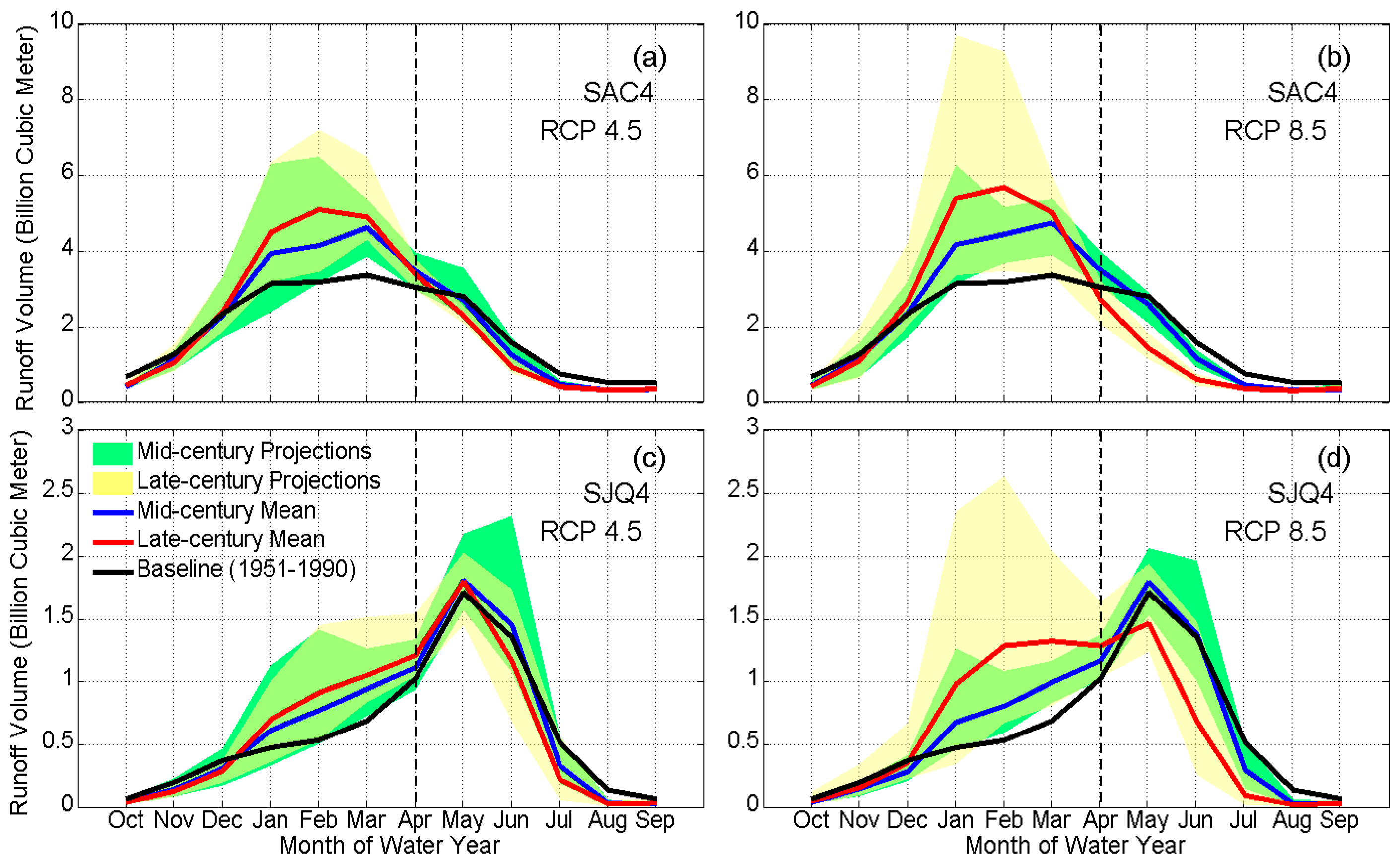
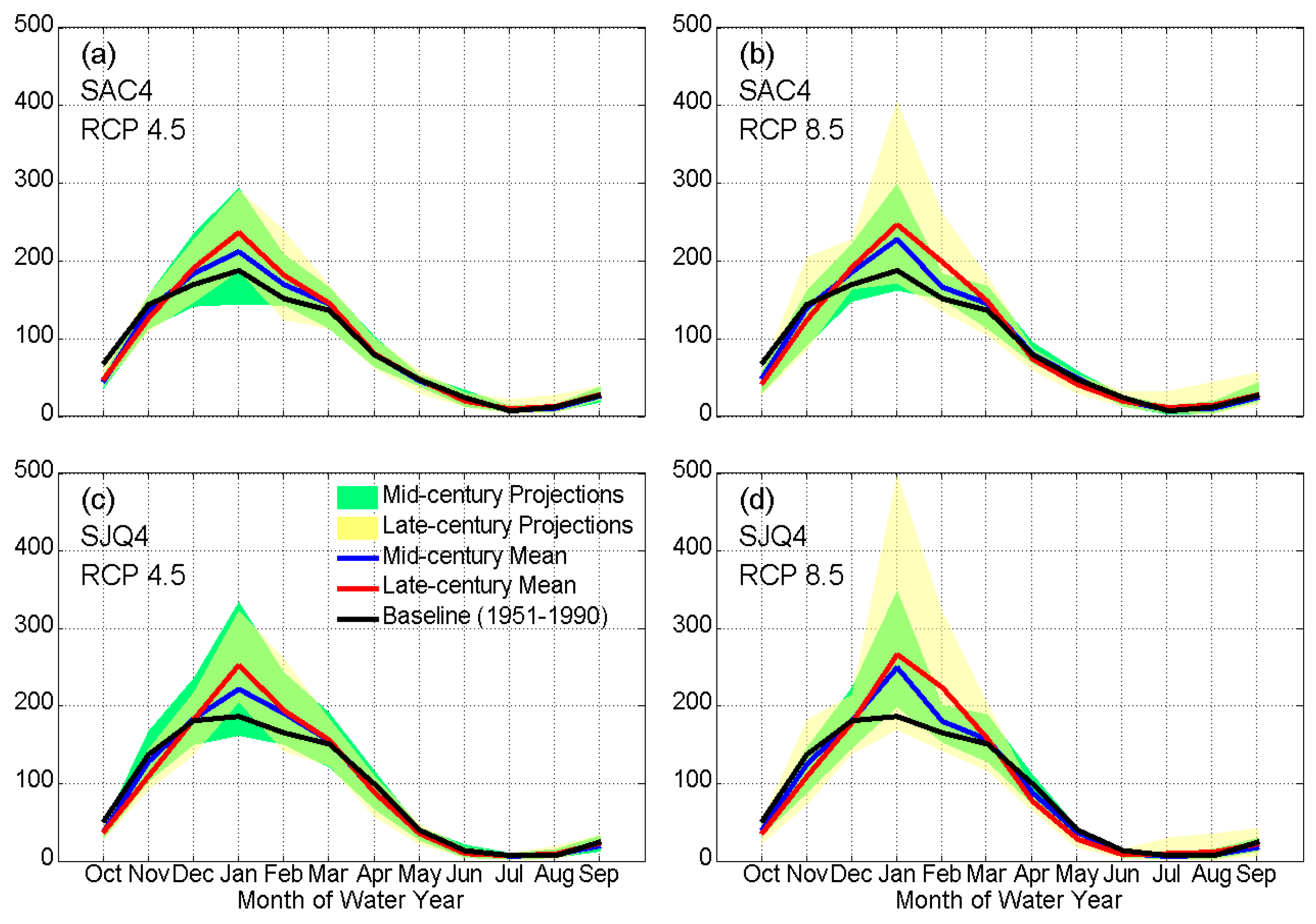
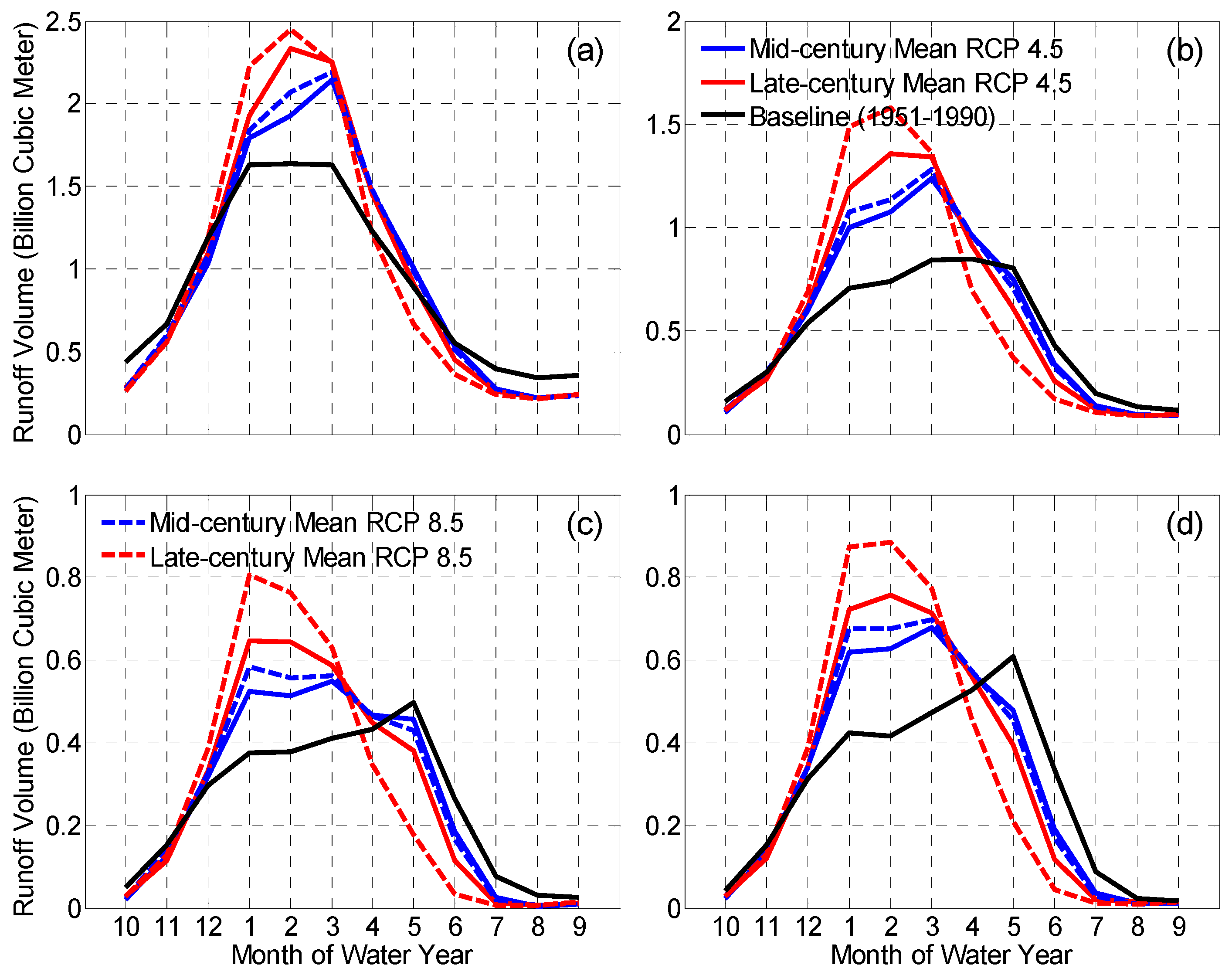
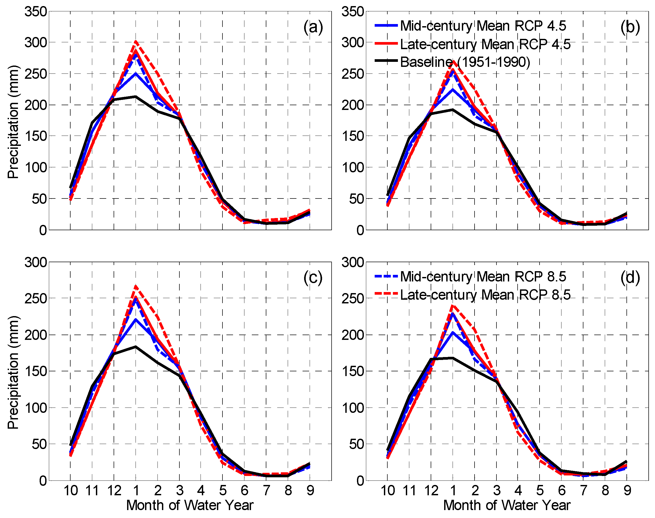
Changes in monthly runoff are examined in terms of monthly pattern, peak volume, and peak timing. Figure 3 shows mean monthly runoff during the historical baseline period and two projection periods (mid-century and late-century), along with projected range (represented by 10 projections under RCP 4.5 or RCP 8.5, respectively) of future monthly runoff. Sacramento Four Rivers (SAC4; Figure 3a,b) and San Joaquin Four Rivers (SJQ4; Figure 3c,d) are used as examples in this case. Corresponding results for individual watersheds are provided in Appendix C (Figure A3 and Figure A4).

Compared to the baseline conditions, mean runoff is expected to increase from January to April for both SCA4 and SJQ4 under both emission scenarios (RCP 4.5 and RCP 8.5). Higher increases are expected during the late-century than in the mid-century. In contrast, less runoff is projected for July–October in both future periods under both emission scenarios for SAC4 and SJQ4. The projected decreases in runoff are more significant in the late-century than its counterpart in the mid-century. There are significant variations between models in projected changes in runoff during the wet months (January–April) for both SAC4 and SJQ4 as well as during the major snowmelt months (May–June) for SJQ4. In comparison, there is more consensus among projections during the dry months (July–October) for both SAC4 and SJQ4 under both emission scenarios. This general pattern (wet months getting wetter and dry months getting drier) is also evident in eight individual watersheds (Figure A3 and Figure A4 in Appendix C).

With respect to peak volume, on average, larger peaks are expected for SAC4 under both emission scenarios (Figure 3a,b). This is particularly the case in late-century for which a 52% increase under RCP 4.5 and a 69% increase in peak runoff under RCP 8.5 are projected. This pattern is also evident for individual Sacramento Valley watersheds (Figure A3 in Appendix C). For SJQ4 (Figure 3c,d), changes in peak volume are much smaller compared to the changes of SAC4. Under RCP 4.5, a 6% increase in peak runoff is projected on average during the mid-century; for late-century, a 5% increase is projected. Under RCP 8.5, a similar increase is expected in mid-century. However, for late-century, peak runoff is projected to decrease by about 14%. This indicates that snowpack would most likely become smaller in late-century under the higher emission scenario (RCP 8.5) due to significant warming expected in this period since snowmelt is a major contributor to the runoff of these watersheds (Table 1). A similar change pattern is observed in individual San Joaquin Valley watersheds (Figure A4 in Appendix C).

In terms of peak timing, no changes are projected for SAC4 during mid-century; however, the peak is projected to shift one month earlier from March to February (Figure 3a,b) by late-century. For individual Sacramento Valley watersheds (Figure A3), on average, runoff is projected to peak earlier except for Sacramento River above Bend Bridge (SBB) during mid-century. For SJQ4, the peak timing is projected to remain unchanged in May in both future periods under both future emission scenarios (Figure 3c,d). This is also the case for individual San Joaquin Valley watersheds (Figure A4) with one exception that Stanislaus River is projected to have an earlier peak during late-century under RCP 8.5. While there are significant variations between projections of individual models, most projections indicate an earlier peak timing for SCA4 and an unchanged peak timing for SJQ4 with few exceptions. The monthly temporal scale in Figure 3 is appropriate for water supply planning. Analyzing changes in peak timing at a finer time scale (e.g., daily) would be more suitable for other purposes including flood management and emergency responses.

Collectively, the projected increases in runoff during the wet season and decreases in runoff during dry season pose challenges to the current water storage management practice and threatens water supply reliability. Additional off-site storages may be required to accommodate projected increases in runoff during the flood season (i.e., before 1 April). The stored water can either be used to recharge depleted groundwater basins or released during the water supply season to meet water demands. The earlier peak runoff projected for the Sacramento Valley watersheds in late-century indicates that management changes might be necessary. For instance, modifications to reservoir operating rules for the flood season could allow greater storage volumes be maintained in order to accommodate the earlier peak runoff. However, such modifications must be made in connection with flood management considerations.

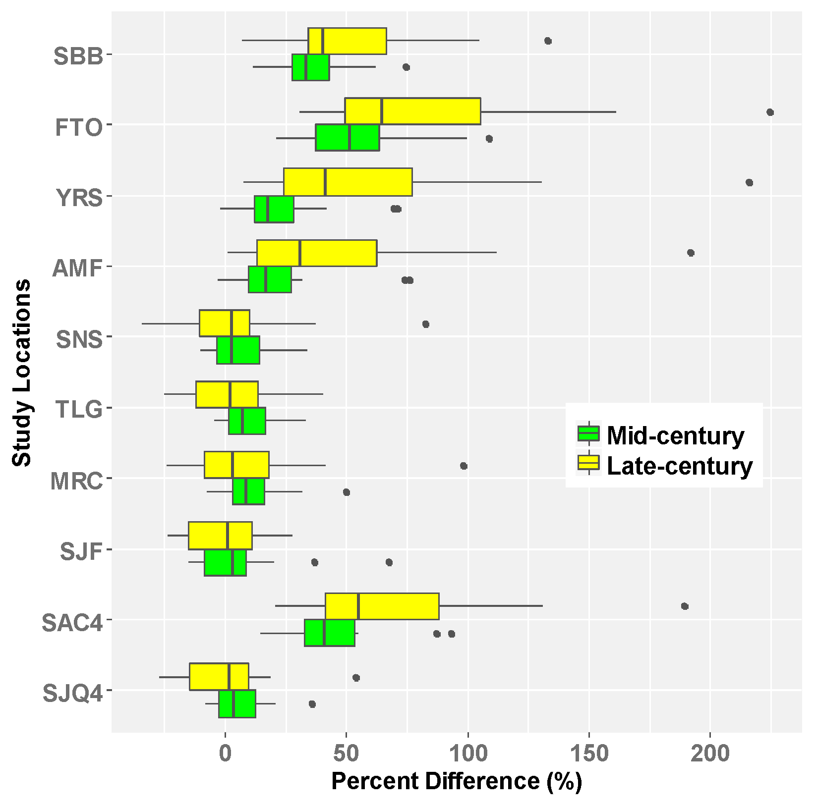
Looking at changes in peak volume for all study locations across all 20 projections (Figure 4), Sacramento Valley watersheds are generally projected to experience larger peaks, particularly for Sacramento River above Bend Bridge (SBB), Feather River (FTO), and Sacramento Four Rivers (SAC4). A few extreme values show over a 150% increase in peak volume during late-century. The extreme values originate from the climate model which projects the most significant increases in future precipitation. For San Joaquin Valley watersheds, median change is generally near or slightly above zero during mid-century, while by late-century there is greater variation among models and more cases of projected decreases in peak volumes. Extreme values for SJQ4 watersheds are all below an increase of 100%. Overall, the range of projected change in peak volume in late-century is larger than mid-century for all study locations, indicative of less agreement among climate projections further into the future because of increasing uncertainty. In addition, the projected change ranges for Sacramento Valley watersheds by late-century are much wider than those of the San Joaquin Valley watersheds, indicative of more uncertainty in the projections of peak runoff in these watersheds. This finding suggests that more adaptive capacity (e.g., additional storage facility) is needed in the Sacramento Valley to accommodate this uncertainty.

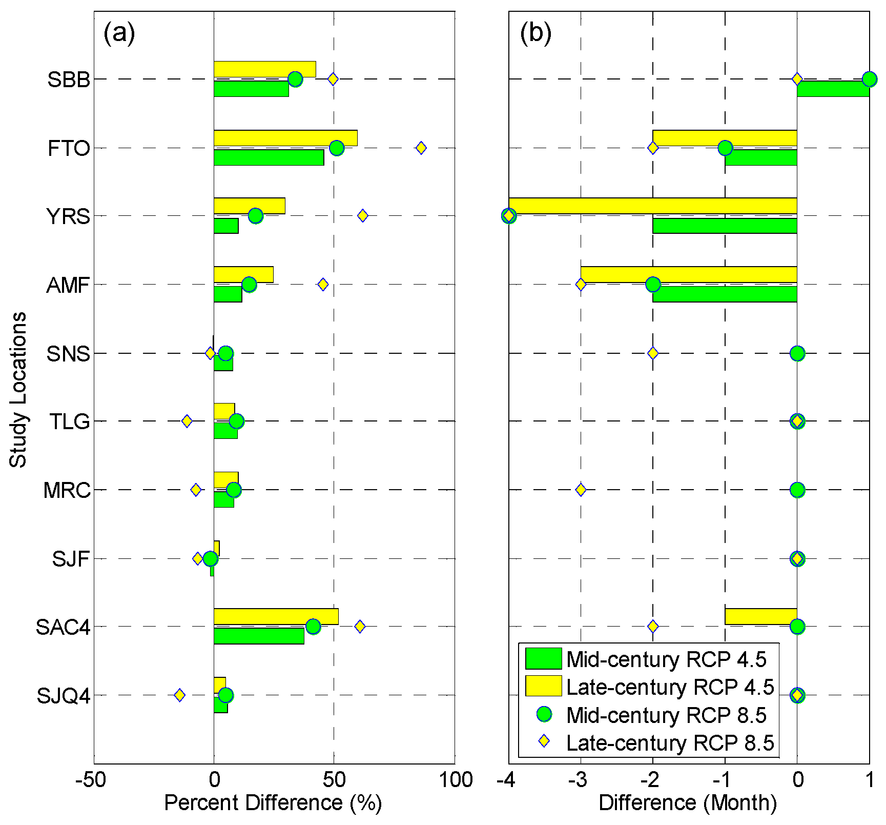
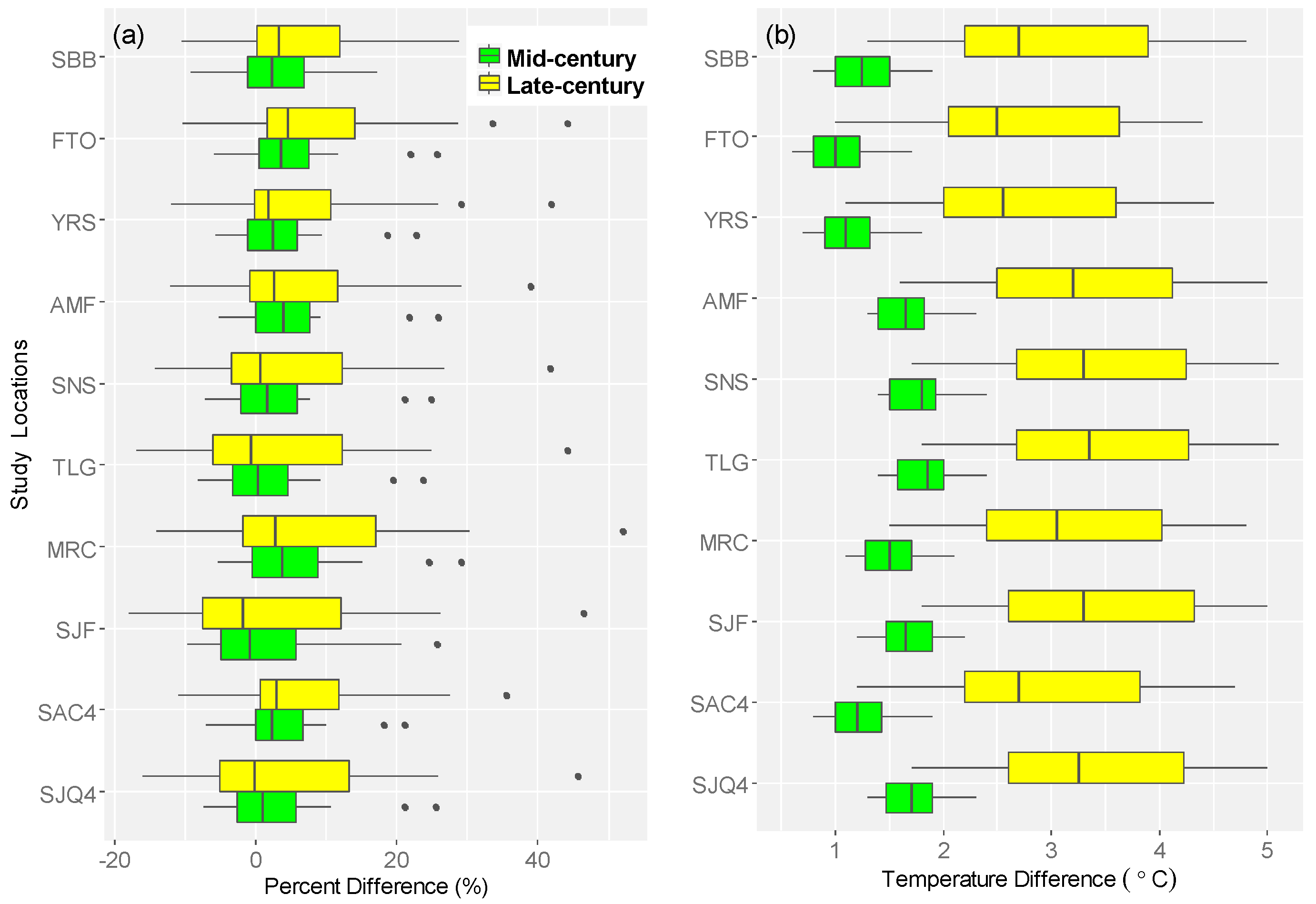
In addition to looking at changes in peak volume of 20 individual projections altogether (Figure 4), the changes are further examined under two different emission scenarios separately. Specifically, the mean of 10 RCP 4.5 projections and mean of 10 RCP 8.5 projections in both future periods are compared with the baseline conditions for all study locations (Figure 5a). For Sacramento Valley watersheds, increases in peak runoff volume are projected in both future periods under both emission scenarios. Increases over the Feather River (FTO) are the most significant. Increases in late-century are higher than their counterparts in mid-century. Comparing two emission scenarios, RCP 8.5 tends to expect higher increases than RCP 4.5. As noted in the Introduction section, atmospheric river (AR) storms contribute largely to the total wet season precipitation in California and serve as a dominant cause of flooding in the state [3]. Particularly, the climatologic peak of AR landfall is at latitudes that impact the Feather River, Yuba River, and American River watersheds. Projections show that the frequency of landfalling ARs in California may increase by about 30% by the end of the 21st century [54]. Increases in the length of AR season, storm temperature, and peak AR intensity along the California coast are also projected [54]. These increases projected in the frequency, duration, and strength of ARs likely lead to increases in peak runoff of Sacramento Valley watersheds. In comparison, changes in projected peak runoff of San Joaquin Valley watersheds are relatively smaller (Figure 5a). The change magnitudes are generally less than 10%. In addition, by late-century under RCP 8.5, peak volumes in the San Joaquin Valley watersheds are projected to decrease. One likely cause of this projected decrease is that peak snowpack under the RCP 8.5 emission scenario is expected to be smaller than its historical counterpart. Those findings are generally in line with what Figure 4 illustrates.

Changes in peak timing on a monthly basis are investigated in a similar way (Figure 5b) as applied to changes in peak volume (Figure 5a). The peak timing of the mean RCP 4.5 and RCP 8.5 projections are compared to their counterparts in the historical baseline period. A negative difference indicates earlier peak while a positive difference means later peak. No difference means no changes in peak timing. Projected changes for San Joaquin Valley watersheds are limited: Under RCP 4.5, no changes in peak timing are projected during both future periods, and under RCP 8.5, only two watersheds (Stanislaus and Merced) tend to have earlier peaks on average. In contrast, changes in Sacramento Valley watersheds are significant. Projected warming likely increases the rain-to-snow ratio during the winter over these watersheds, leading to generally earlier runoff peak. For Feather (FTO), Yuba (YRS), and American River (AMF) watersheds, earlier peaks are projected, particularly for late-century under RCP 8.5 scenario. For Sacramento River above Bend Bridge, however, later peaks (one month later) are projected during mid-century while no changes are projected during late-century. Looking at Sacramento four rivers together (SAC4), no changes are projected in mid-century while earlier peaks are projected during late-century. Potential causes of these changes are discussed in the Discussion section (Section 4).

Figure 5b sheds light on changes in peak timing by comparing the mean of individual projections to the baseline. The changes associated with individual projections are also examined to give a more complete picture of the number of projections showing changes in peak timing, cataloged by change magnitude (in months), analysis period, and emission scenario (

Table 2. Number of RCP4.5 and RCP8.5 projections out of 10 GCM projections showing changes in peak runoff timing from the baseline ¹.

ID	Mid-Century						Late-Century
	−4	−3	−2	−1	0	1	−4	−3	−2	−1	0	1
SBB	0/02	0/0	0/0	0/1	3/3	7/6	0/0	0/0	0/0	0/1	7/6	3/3
FTO	0/0	0/1	2/1	7/8	1/0	0/0	0/0	1/3	4/3	5/4	0/0	0/0
YRS	3/5	1/1	3/3	2/1	1/0	0/0	5/5	3/3	2/2	0/0	0/0	0/0
AMF	2/2	2/2	3/5	2/1	1/0	0/0	2/3	5/3	3/4	0/0	0/0	0/0
SNS	0/0	0/0	0/1	0/0	10/9	0/0	0/2	0/3	1/4	0/1	9/0	0/0
TLG	0/0	0/0	0/0	0/0	10/10	0/0	0/0	0/2	0/0	0/0	10/8	0/0
MRC	0/0	0/0	0/0	0/0	9/7	1/3	0/0	0/3	0/2	0/0	10/5	0/0
SJF	0/0	0/0	0/0	0/0	4/5	6/5	0/0	0/1	0/0	0/0	9/9	1/0
SAC4	0/0	0/0	0/1	3/2	7/7	0/0	0/0	0/0	1/3	5/3	4/4	0/0
SJQ4	0/0	0/0	0/0	0/0	9/9	1/1	0/0	0/2	0/1	0/0	10/7	0/0

¹ Unit is in month; 0 indicates no changes; negative and positive numbers indicate peaking earlier and later, respectively. ² The first number is for RCP 4.5 scenario; the second number is for RCP 8.5 scenario.

). For San Joaquin Valley watersheds, no RCP 4.5 or RCP 8.5 projections show earlier peaks with one exception (one RCP 8.5 projection for SNS) during mid-century. Most projections show no changes in peak timing during this period except for the San Joaquin River (SJF) where about half of projections are projected to peak one month later. During late-century, all but one (for SJF under RCP 4.5) projections show no changes. Under RCP 4.5, a majority of projections indicate no changes in peak timing from the baseline. However, under RCP 8.5 during the same period, a number of projections show earlier peaks particularly for the Stanislaus River (SNS) where the peaks of all projections are expected to occur one-to-four months earlier. Looking at four rivers together (SJQ4), most projections show peak timing to be in the same month as the historical baseline.

Nearly all projections show changes in peak timing for Sacramento Valley watersheds (Table 2). During mid-century, all RCP 8.5 projections show earlier peaks in Feather, Yuba, and American River watersheds, which is also the case for most (9 out of 10) RCP 4.5 projections. During late-century, all RCP 4.5 and RCP 8.5 projections are projected to peak even earlier in these three watersheds. In comparison, for Sacramento River above Bend Bridge, only one RCP 8.5 projection tends to peak one month earlier during both future periods. Most projections (7 RCP 4.5 and 6 RCP 8.5 projections) show a change in peak timing to one month later for this watershed during mid-century and show no changes in peak timing during late-century. For Sacramento Four Rivers (SAC4), no changes are expected under most projections during mid-century; however, during late-century, more than half of the runoff projections are expected to peak earlier. Overall, those observations are largely in line with what Figure 5b illustrates.

In short, notable increases in peak runoff volume are projected for Sacramento Valley watersheds. Increases in late-century under RCP 8.5 are higher than their counterparts in mid-century under RCP 4.5. Increases are also projected for San Joaquin Valley watersheds. However, the amount of increase in San Joaquin Valley watersheds is generally within the range of model biases (

Table A2. Summary of VIC model calibration and validation statistics.

Watershed ID	Calibration (1970–2003)					Validation (1922–1969)
	Percent Bias (%)	R2		NSE		Percent Bias (%)	R2		NSE
		Monthly	Annual	Monthly	Annual		Monthly	Annual	Monthly	Annual
SBB	4.15	0.96	0.98	0.90	0.92	2.99	0.96	0.97	0.90	0.94
FTO	11.37	0.94	0.96	0.89	0.90	10.93	0.89	0.98	0.82	0.91
YRS	6.57	0.94	0.98	0.90	0.96	4.40	0.88	0.97	0.84	0.96
AMF	5.28	0.89	0.98	0.84	0.97	4.31	0.86	0.98	0.82	0.97
SNS	16.54	0.92	0.97	0.83	0.86	17.80	0.89	0.98	0.82	0.77
TLG	−2.61	0.92	0.99	0.88	0.98	1.68	0.92	0.98	0.89	0.96
MRC	4.78	0.88	0.99	0.86	0.96	13.66	0.89	0.98	0.84	0.84
SJF	−6.67	0.89	0.99	0.85	0.96	−1.25	0.91	0.95	0.86	0.93

in Appendix B). For Sacramento Valley watersheds, except for the Sacramento River above Bend Bridge, runoff is projected to peak earlier particularly during late-century under RCP 8.5. In comparison, no changes in peak timing are projected for San Joaquin Valley watersheds under most projections.

3.2. Changes in Seasonal and Annual Runoff

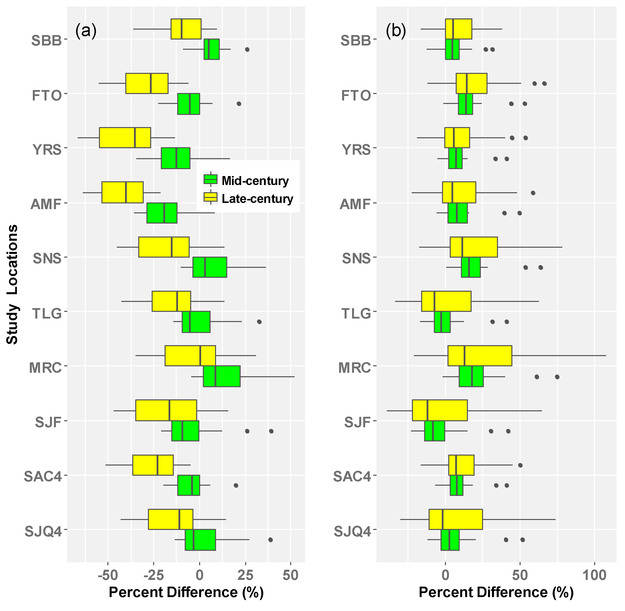
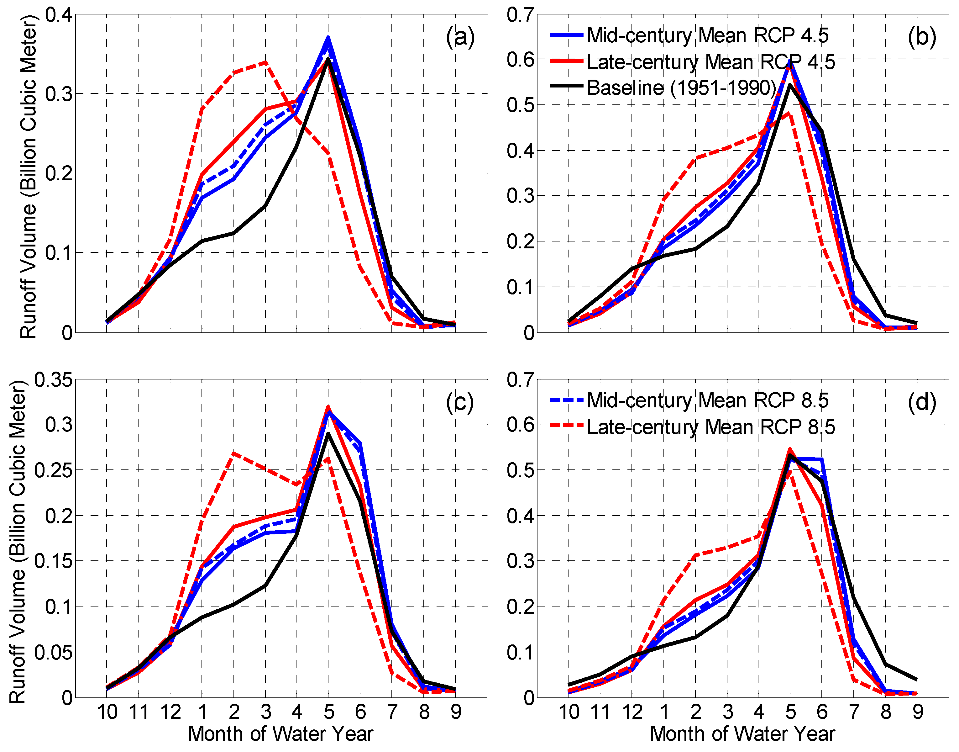
This section examines changes in projected April–July runoff and annual runoff from the baseline condition. Figure 6 illustrates the full range of the differences between 20 individual RCP 4.5 and RCP 8.5 projections and the baseline for each study location in two future periods. For April–July runoff (Figure 6a), a majority of projections during late-century show decreases. This is particularly true for Feather (FTO), Yuba (YRS), American (AMF), and Sacramento four rivers (SAC4) where all 20 projections consistently exhibit decreases in April–July runoff. The largest decrease (around −65%) is projected for the Yuba watershed (YRS). For mid-century, most projections exhibit increases in April–July runoff over Sacramento River above Bend Bridge (SBB), Stanislaus (SNS), and Merced (MRC); it is the opposite for other study locations. The largest increase (slightly above 50%) is projected for the Merced (MRC) watershed. Overall, the variation ranges are generally large for all study locations in both future periods. The ranges in late-century are even larger than their counterparts during mid-century, which is expected since uncertainty in climate projections tends to become larger further into the future. This is also evident for annual runoff (Figure 6b). Comparing Sacramento Valley watersheds to San Joaquin Valley watersheds, variations in the latter are generally higher. This suggests that climate models tend to agree less with each other on potential future climate over San Joaquin Valley watersheds which are more dominated by snowmelt (versus Sacramento Valley watersheds). The largest increase (over 100%) in annual runoff is projected for Merced (MRC). On average, except for Tuolumne (TLG) and San Joaquin (SJF), other locations are expected to experience more runoff on the annual scale. These findings are further discussed in the Discussion section (Section 4).

In addition to looking at the potential range of future changes in April–July runoff and annual runoff, the number of projections showing positive changes is summarized to illustrate the level of consensus among different climate projections on the change signal (

Table 3. Number of RCP 4.5 and RCP 8.5 projections out of 10 GCM projections showing increases in April–July and annual runoff.

ID	AJ				Annual
	Mid-Century		Late-Century		Mid-Century		Late-Century
	RCP 4.5	RCP 8.5	RCP 4.5	RCP 8.5	RCP 4.5	RCP 8.5	RCP 4.5	RCP 8.5
SBB	9	8	5	0	8	7	8	7
FTO	3	2	0	0	9	10	9	9
YRS	3	0	0	0	8	9	8	6
AMF	1	0	0	0	8	9	8	5
SNS	6	6	3	0	10	10	9	8
TLG	4	4	3	2	2	4	3	4
MRC	8	9	8	3	9	9	9	7
SJF	3	2	3	2	2	3	3	3
SAC4	3	2	0	0	8	9	8	7
SJQ4	5	4	3	2	7	6	5	4

). For Feather (FTO), Yuba (YRS), American (AMF), and Sacramento Four Rivers (SAC4), the increasing signal is generally weak in April–July runoff particularly during late-century when no projections show increases. For Sacramento River above Bend Bridge (SBB) and Merced (MRC), however, a majority of projections show increases in April–July runoff during mid-century. In general, fewer projections indicate increases in late-century (versus mid-century) under RCP 8.5 (versus RCP 4.5). Particularly, no projections show increases in April–July runoff over any Sacramento Valley watersheds during late-century under RCP 8.5. For annual runoff, most projections exhibit increases in Sacramento Valley watersheds as well as Stanislaus (SNS) and Merced (MRC), while the consensus is lower for Tuolumne (TLG) and San Joaquin (SJF). This is generally consistent with what Figure 6 illustrates.

In summary, large variations in future April–July runoff and annual runoff are projected. Variations are even larger during late-century compared to their counterparts in mid-century. However, most projections indicate decreases in April–July runoff for Feather River (FTO), Yuba River (YRS), American River (AMF), and San Joaquin River (SJQ); most projections show slight increases in annual runoff for all watersheds except for Tuolumne River (TLG) and San Joaquin River (SJQ). The change rates (% change from the baseline) are generally higher during late-century (versus mid-century) under RCP 8.5 (versus RCP 4.5).

3.3. Trend Analysis

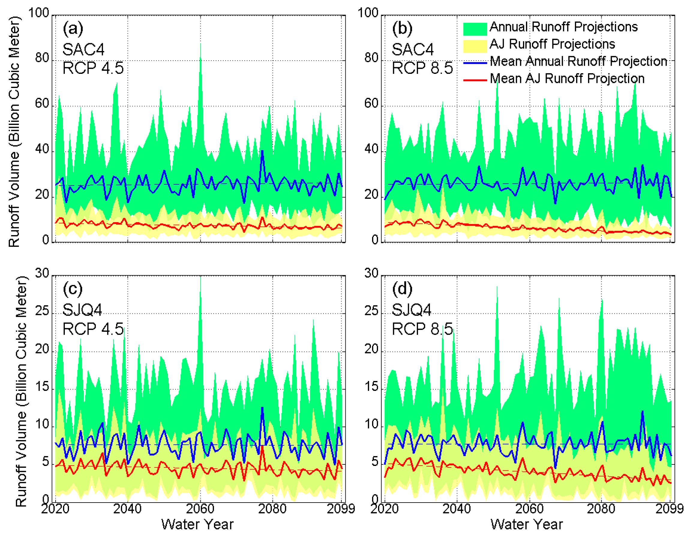
Aside from relative changes from the baseline, the overall change pattern (increasing, decreasing, or no change) is also investigated during the entire projection period 2020–2099. Figure 7 illustrates all projections on April–July runoff and annual runoff, mean of these projections, and the trend lines of the mean values for Sacramento Four Rivers (SAC4; Figure 7a,b) and San Joaquin Four Rivers (SJQ4; Figure 7c,d). Large year-to-year variations are evident under both emission scenarios. Large variations also exist across different projections. It is also evident that April–July runoff accounts for a larger portion of the annual runoff for San Joaquin Four Rivers other than Sacramento Four Rivers. For the mean projection on annual runoff, the changing trend is not pronounced for San Joaquin Four Rivers. For Sacramento Four Rivers, an increasing trend can be observed. For the mean projection on April–July runoff, a decreasing trend is notable for both study locations under both emission scenarios particularly under RCP 8.5.

The specific changing rate (slope of the trend line) is determined for SJQ4 and SAC4 as shown in Figure 7 along with individual watersheds in Sacramento Valley and San Joaquin Valley (

Table 4. Trend slope and corresponding p-values for mean projections on April–July and annual runoff.

ID	Scenario	April–July Runoff (AJ)		Annual Runoff (A)		AJ/A
		Slope (MCM/Year)	p-Value	Slope (MCM/Year)	p-Value	Slope (/Decade)	p-Value
SBB	RCP 4.5	−5.9	<0.001	3.7	0.5	−0.007	<0.001
	RCP 8.5	−15.2	<0.001	2.6	0.8	−0.02	<0.001
FTO	RCP 4.5	−6.7	<0.001	2.8	0.5	−0.01	<0.001
	RCP 8.5	−15.0	<0.001	3.6	0.3	−0.03	<0.001
YRS	RCP 4.5	−4.1	<0.001	0.5	0.8	−0.02	<0.001
	RCP 8.5	−10.1	<0.001	0.6	0.8	−0.04	<0.001
AMF	RCP 4.5	−4.3	<0.001	−0.4	0.9	−0.01	<0.001
	RCP 8.5	−10.3	<0.001	−0.5	0.9	−0.03	<0.001
SNS	RCP 4.5	−2.3	<0.001	−0.4	0.8	−0.02	<0.001
	RCP 8.5	−6.7	<0.001	−1.0	0.4	−0.04	<0.001
TLG	RCP 4.5	−2.1	0.04	−0.6	0.7	−0.01	<0.001
	RCP 8.5	−6.8	<0.001	−0.4	0.8	−0.03	<0.001
MRC	RCP 4.5	−1.2	0.06	−0.3	0.9	−0.009	<0.001
	RCP 8.5	−4.1	<0.001	−0.3	0.8	−0.03	<0.001
SJF	RCP 4.5	−2.3	0.04	−1.1	0.6	−0.01	<0.001
	RCP 8.5	−6.0	<0.001	−0.6	0.6	−0.03	<0.001
SAC4	RCP 4.5	−20.7	<0.001	7.5	0.6	−0.01	<0.001
	RCP 8.5	−50.9	<0.001	7.1	0.6	−0.02	<0.001
SJQ4	RCP 4.5	−8.3	0.02	−1.8	0.8	−0.01	<0.001
	RCP 8.5	−23.7	<0.001	−2.5	0.6	−0.04	<0.001

). April–July runoff tends to decrease under both emission scenarios for all study locations. These decreasing trends are all statistically significant at a significance level of 0.05 except for one case (Merced River, p = 0.06). The decreasing rates are generally higher under RCP 8.5 than their RCP 4.5 counterparts. Comparing to San Joaquin Valley watersheds, Sacramento Valley watersheds generally have higher decreasing rates. For annual runoff, a slight decreasing trend is detected for all San Joaquin Valley watersheds. In comparison, all Sacramento Valley watersheds except for American (AMF) show increasing trend. However, none of these trends in annual runoff is statistically significant (p > 0.05). The trend in the April–July runoff over annual runoff ratio is also examined. The ratio tends to decrease significantly in the projection period under both emission scenarios across all study watersheds, suggesting less snowmelt contribution to annual runoff further into the future. The decreasing rates under RCP 8.5 are higher than the decreasing rates under RCP 4.5.

In addition to trends in mean projections (Table 4), trends in individual projections and observed runoff are also assessed. For annual runoff, no statistically significant trends are identified in observed runoff for those study locations except for Sacramento River above Bend Bridge (SBB; slope: 31.8 million cubic meters (MCM)/year; p-value: 0.05) during a history period (1920–1999) with the same length as the projection period (2020–2099). No RCP 4.5 projections show any trends on annual runoff over the projection period. However, one RCP 8.5 projection (GFDL-CM3) indicates significant increasing trends at all study locations. Another RCP 8.5 projection (ACCESS1-0) shows a decreasing trend for all study locations except for San Joaquin River watershed (SJF). A third RCP 8.5 projection (CESM1-BGC) exhibits slight increasing trends at Merced (MRC) and San Joaquin River watershed (SJQ). Other RCP 8.5 projections on annual runoff have no significant trends.

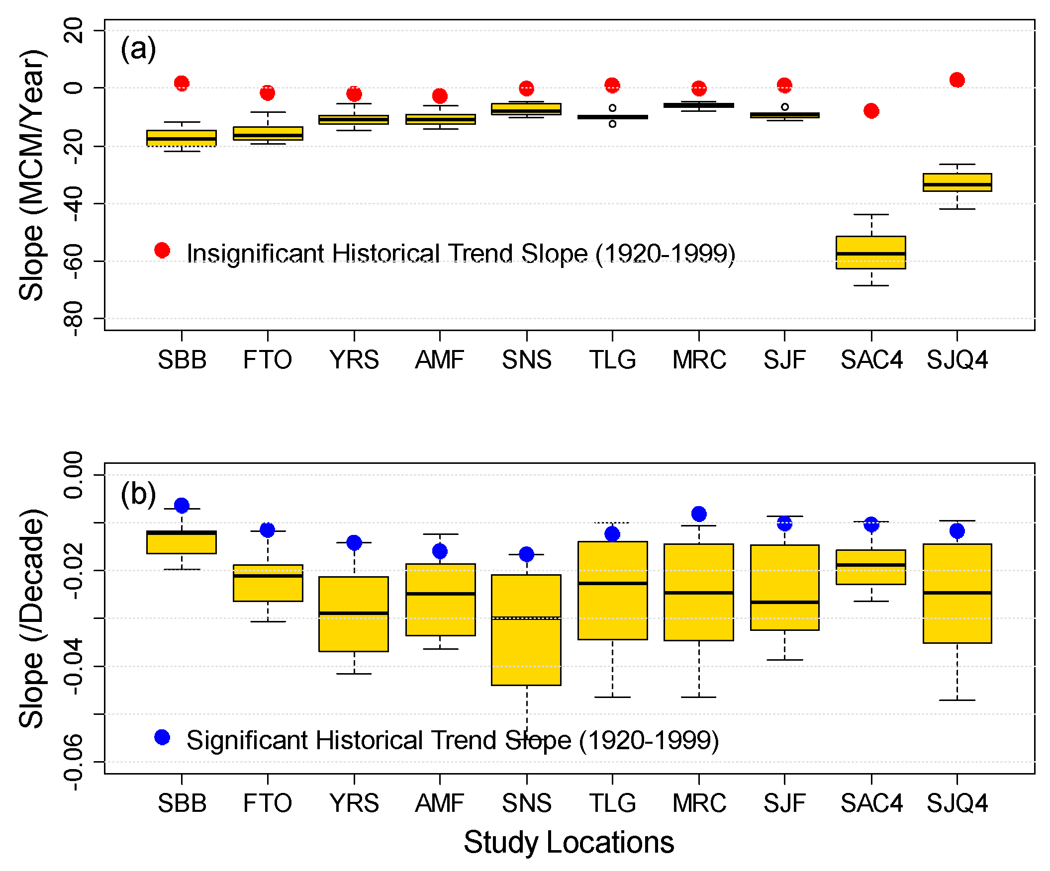
For April–July runoff (Figure 8a), there are slightly increasing or decreasing trends in the historical (1920–1999) values at all study locations. However, none of them is statistically significant. More than half of the projections (12, 14, 14, 13, and 12 out of 20 for SBB, FTO, YRS, AMF, and SAC4, respectively) for Sacramento Valley watersheds show significant decreasing trends. In comparison, only about one third to half of the projections (11, 7, 7, 6, and 7 for SNS, TLG, MRC, SJF, and SJQ4, respectively) have significant decreasing trends for San Joaquin Valley watersheds. This implies that the impacts of warming on snowpack (and thus April–July runoff) are expected to be more pronounced in Sacramento Valley watersheds rather than in San Joaquin Valley watersheds. The latter are located in higher elevations with higher resilience to warming than the lower-elevation Sacramento Valley watersheds. Comparing decreasing rates in historical and projection periods, the latter are generally higher. For April–July runoff over annual runoff ratio (Figure 8b), it has a significant decreasing tendency during the historical period for all watersheds. During the projection period, most projections (ranging from 14 for SBB to 19 for YRS) show significant decreasing trends. The decreasing rates in the projection period are generally larger compared to their historical counterparts.

In a nutshell, statistically significant trends are not evident in projected annual runoff for most watersheds. On average, however, April–July runoff is projected to decrease particularly under RCP 8.5. April–July runoff over annual runoff ratio is also projected to decrease. The decreasing rates are expected to be higher than their corresponding historical decreasing rates, indicating less contribution of snowmelt to total annual runoff further into the future.

4. Discussions

There are many sources of uncertainty associated with assessing changes in future runoff projections from the historical baseline. Firstly, climate change science has its uncertainties which are often associated with climate models (and their parameterization and initial conditions) used to project future climate and future development (emission) scenarios. To address them, this study looks at a suite of 20 climate projections suitable for California water resources planning activities rather than favoring a single climate model under a single emission scenario. Secondly, there is uncertainty involved in the process of converting climate projections to runoff projections. This study applies the VIC model which takes temperature and precipitation produced by climate model projections as input and generates corresponding runoff projections. The VIC model configuration does not reflect the real watershed characteristics perfectly, as is evident in the calibration results (Appendix B). Thirdly, the selection of a benchmark baseline adds uncertainty since certain historical periods are wetter (or drier) than others. This section discusses these uncertainties, potential causes of the changes reported in the previous section, the scientific and operational value of the study and recommendations for future work.

4.1. Climate Projections

There are large uncertainties on how future precipitation differs from the historical baseline (Figure A5 in Appendix C) [44,55]. There is no consensus among projections which would indicate a wetter (positive difference) or drier (negative difference) condition. The difference generally varies in a wide range at each location, which is particularly the case during late-century. The large uncertainties in precipitation projections cascade to larger variations in runoff projections, which is further discussed in Section 4.4.

In contrast, there is a clear warming signal in all temperature projections (Figure A5 Appendix C) [44], though the warming magnitude varies across different projections and two different future periods. In general, higher increases in temperature and larger variation ranges are projected for late-century rather than in mid-century. On average, the Sacramento Valley (represented by SAC4) is expected to experience slightly less warming than the San Joaquin Valley (represented by SJQ4). This warming pattern also has implications on runoff projections, which will also be further elaborated in Section 4.4.

4.2. VIC Model

The VIC model has been widely used in assessing hydrological impacts of climate change in California. For example, Maurer and Duffy [16] used the VIC model to project future runoff at eight watersheds in California. The study concluded that decreases in summer flows, increases in winter flows, and earlier runoff are expected. In a follow-up study, Maurer [17] used a newer set of 11 GCM projections to drive the VIC model and produced streamflow projections from 2071–2100 for four watersheds in California. The study projected declines in end-of-winter snowpack. Cayan et al. [40] applied the VIC model in simulating snow responses to warming projections in California. They found out that snow losses increase with warming and are most severe in projections corresponding to the highest emissions. Gergel et al. [36] utilized VIC in modeling future snowpack and soil moisture across the Western U.S. including the Sierra Nevada region in California. A decline in mountain snowpack, an advance in the timing of spring melt, and a reduction in the length of the snow season were projected. Other hydrological models including the soil and water assessment tool (SWAT) and Sacramento Soil Moisture Account (SAC-SMA) model have also been explored in generating runoff projections in Sierra Nevada watersheds [19]. Earlier shift in peak snowmelt runoff, decreased occurrence of wet hydrologic years, and more frequent drought conditions were expected. Qualitatively speaking, the findings of these previous studies are largely in line with those of the current study. However, the current study extended these previous studies in that (1) it used the latest available operative climate projections (representing the state-of-the-art climate science) in driving the VIC model; (2) it focused on a range of variables (e.g., April–July runoff) that are routinely used in DWR’s water resources planning and management practices.

Despite its popularity in assessing climate change impacts on hydrologic variables [38,39], the VIC model is not free from uncertainties. There are uncertainties associated with model structure, parameterization, and assumptions. For instance, one major structural simplification of the VIC model is that it defines three soil zones to simulate the vertical movement of soil moisture rather than explicitly considering groundwater. However, in the current work where the study areas are all mountainous headwater watersheds without substantial surface water and groundwater regulations, exclusion of deeper groundwater would not impact the results of the study given that there are other larger uncertainties. The structural imperfectness may be partially compensated by model parameters. The calibrated parameters yield satisfactory model performance during the calibration and validation periods (Figure A1 and Figure A2; Table A2 in Appendix B). Nevertheless, the model is still biased and tends to overestimate runoff particularly during wet years. The perception of model bias has to be taken into account in any practical decision-making processes. Additionally, the model assumes stationarity in topography, soil types, land use, vegetation classes, and water management practices. This assumption may not hold valid throughout the projection period. The model further assumes that future wind speed (which is required as a VIC model input) would be identical to the historical conditions. This may not necessarily be the case. However, as of now, no downscaled projections on future wind speed are produced for water resources planning studies across California. In the VIC model, wind speed impacts the calculation of canopy evaporation which is normally not a major component of the water budget. In light of that, it is a common practice to apply the historical wind speed data instead [18]. Projected wind speed data will be used in our future studies should they become available.

4.3. Historical Baseline

This study uses water year 1951–1990 as the baseline period when assessing changes in peak runoff, seasonal runoff, and annual runoff in two future periods (mid-century and late-century). This is mainly due to the fact that the raw climate projections are downscaled based on historical data available from calendar year 1950–2013 via the LOCA method [32]. During this historical period (1950–2013), water year 1951–1990 is relatively less impacted by anthropogenic climate change (warming) than other 40-year sub-periods. It is possible that a different baseline period (e.g., 1901–1940) without significant anthropogenic impacts may yield different results. This will be investigated when a longer data record becomes available.

In previous relevant studies [18,56], VIC simulations in the historical period are often applied as the baseline against which future VIC model projections are compared. The current study uses observed runoff in the historical period as the baseline. This is necessary from an operational perspective. The water infrastructure across California (including the SWP and CVP) is designed using historical hydro-climatic data which are deemed as “ground truth”. Benchmarking future projections against historical observations informs practical decision-making, with the perception that future projections contain uncertainty. For instance, assuming that the current system can exactly handle the peak runoff observed, a projected 10% increase (from the observation rather than model simulation) in future peak runoff would require new (e.g., 10% more) system storage or corresponding system re-operation to cope with. Notwithstanding, when historical observations are not available (which is not the case of this study), model simulations can be applied to facilitate decision-making in practice.

4.4. Attribution of Changes

Firstly, the study indicates that watershed characteristics strongly affect peak runoff responses to climate change. Sacramento Valley watersheds are rain-dominated due to their relatively lower elevations compared to San Joaquin Valley watersheds (Figure 1; Table 1). The higher elevation distribution in San Joaquin Valley watersheds serves as a natural buffer to climate change (warming) and enables a redistribution of the snowpack. Warmer temperatures that are still below freezing can facilitate greater snowpack accumulation as there can be more atmospheric moisture available in an overall warming environment for precipitation formation. This causes resistance to change in runoff volume and timing in San Joaquin Valley watersheds. A recent study [57] also reports that, due to their elevation differences, the northern Sierra Nevada exhibits higher hydrologic vulnerability to warming than in the southern region.

In terms of peak volume, the study shows that it is projected to increase for Sacramento Valley watersheds. Increases are higher during late-century (versus mid-century) under RCP 8.5 (versus RCP 4.5). In comparison, increases in runoff are also projected for San Joaquin Valley watersheds except for late-century under higher emission scenario. However, the increases are significantly smaller in magnitude due to above-mentioned resilience unique to San Joaquin Valley watersheds. Increases in peak runoff are likely caused by projected increases in peak precipitation. Figure 9 illustrates precipitation projections for Sacramento Four Rivers and San Joaquin Four Rivers. It is noticeable that increases are projected in both peak monthly precipitation and wet season precipitation. These are also observed in projections for eight individual watersheds (Figure A6 and Figure A7 in Appendix C). Increases in California’s wet extremes in the 21st century are also projected in previous studies [8,58] as well as the frequency and intensity of atmospheric river storms [3,54]. It should be highlighted that significant warming is projected for late-century under RCP 8.5 (Figure A5). This may overpower the natural resilience of San Joaquin Valley watersheds and contribute to smaller snowpack and trigger earlier snowmelt. Both factors collectively may lead to smaller runoff peaks for those watersheds under RCP 8.5 in late-century.

In terms of peak timing, the study indicates that for Feather River, Yuba River, and American River watersheds, earlier (than historical) peaks are projected. Earlier peaks are also projected for Sacramento River above Bend Bridge during late-century. Earlier peak of Sacramento basin runoff is also reported in a recent study [59] which looks at daily runoff projections derived from those 20 climate projections applied in the current study. For San Joaquin Valley watersheds, however, the peak timing is expected to largely remain in the same month. Figure 9 shows that precipitation peak timing is expected to remain unchanged (during January) from historical conditions. This is also the case for individual watersheds (Figure A6 and Figure A7 in Appendix C). Therefore, these earlier runoff peaks are most likely not caused by shifts in precipitation peak timing. Instead, these changes are likely linked to the natural resilience to warming as mentioned above.

To make it clear, Figure 10 depicts projected monthly temperature over Sacramento Four Rivers and San Joaquin Four Rivers. In general, warming is expected across all months in both future periods. Particularly, warming in late-century is expected to be more significant than warming in mid-century. In addition, the warming signal tends to be stronger during the summer months than during the winter months. However, warming during the winter has more implications than warming in the summer from a water supply’s perspective. In California, a majority of the state’s annual water supply occurs as wintertime precipitation. Warming in the winter has shown to elevate the rain-snow elevation and lead to a higher ratio of the precipitation falling as rain rather than snow [60,61]. For rain-dominated watersheds with relatively lower elevations (e.g., Sacramento Valley watersheds; Table 1), increased rainfall around the normal rain-snow elevation (when there is no significant warming) would contribute to runoff at watershed outlet quickly. This will likely shift the peak runoff timing earlier in those watersheds, particularly during late-century when projected significant warming is expected to further elevate the rain-snow elevation and increase the rain-over-snow ratio. For snow-dominated watersheds located in relatively high elevations (e.g., San Joaquin Valley watersheds; Table 1), a majority of the precipitation is expected to continue falling as snowfall despite the increasing rain-over-snow ratio. Large snowpack is expected to continue building up in high elevations and melt during late-spring and early summer, particularly under RCP 4.5 where the warming is moderate relatively speaking. In this case, snowmelt would continue to be the major contributor of the peak runoff in San Joaquin Valley watersheds. The peak runoff timing likely remains unchanged at the monthly time scale.

It should be pointed out that Sacramento River above Bend Bridge (SBB) runoff is shown to peak one month later (Figure 5b) during mid-century. One likely cause is that the watershed contains volcanic deposits that buffer runoff extremes. Additional rainfall (more precipitation falling as rainfall) driven runoff and earlier snowmelt caused by mid-century warming for SBB may be detained in volcanic deposits and released later. Another reason is that the historical SBB runoff peaks in February (Figure A3). However, March runoff is very close to the peak runoff with a difference at 0.37%. Looking at finer scale (e.g., weekly or daily), it is very likely that the peak timing remains unchanged. This will be investigated in a follow-up study using daily runoff projections.

Secondly, the study shows that some changes are common to both Sacramento Valley and San Joaquin Valley watersheds, despite their elevation differences. Specifically, the study indicates that wet months (March–October) tend to get wetter and dry water supply months (April–July) are projected to be even drier in terms of runoff amount. This is likely to be a “new normal” for future runoff in California [62]. One likely cause is that wet season precipitation is projected to increase slightly while dry season precipitation is projected to decrease.

Table 5. Percent difference of mean projection on October–March and April–July precipitation from the historical baseline.

ID	Scenario	October–March Precipitation (%)		April–July Precipitation (%)
		Mid-Century	Late-Century	Mid-Century	Late-Century
SBB	RCP 4.5	3.4	7.7	−1.5	−0.3
	RCP 8.5	5.9	9.5	−1.1	−7.1
FTO	RCP 4.5	5.2	10.2	−0.6	−0.6
	RCP 8.5	7.8	13.6	0.2	−8.6
YRS	RCP 4.5	3.0	7.4	−1.9	−2.2
	RCP 8.5	5.7	10.7	−0.6	−10.1
AMF	RCP 4.5	4.3	7.4	1.8	1.1
	RCP 8.5	6.7	10.9	2.2	−8.6
SNS	RCP 4.5	4.4	6.6	−7.5	−8.4
	RCP 8.5	6.5	10.4	−8.1	−18.5
TLG	RCP 4.5	4.0	5.7	−9.8	−10.3
	RCP 8.5	5.7	10.0	−10.8	−21.1
MRC	RCP 4.5	7.6	9.7	−8.0	−9.7
	RCP 8.5	9.6	14.3	−9.3	−21.3
SJF	RCP 4.5	5.1	6.2	−15.1	−16.4
	RCP 8.5	6.6	11.0	−16.7	−28.2
SAC4	RCP 4.5	4.0	8.3	−0.9	−0.3
	RCP 8.5	6.5	10.9	−0.3	−7.9
SJQ4	RCP 4.5	5.1	6.8	−10.5	−11.6
	RCP 8.5	6.9	11.2	−11.7	−22.6

tabulates differences between mean projection and the historical baseline during the wet season (October–March) as well as the dry water supply season (April–July) for each study location under two emission scenarios. In general, during mid-century, October–March precipitation is projected to increase from 3.0% (Yuba River under RCP 4.5) to 9.6% (Merced River under RCP 8.5). During late-century, the increase range is from 5.7% (Tuolumne River under RCP 4.5) to 14.3% (Merced River under RCP 8.5). These increases in wet season precipitation may contribute to increases in wet season runoff. For April–July precipitation, however, decreases are mostly projected particularly during late century (e.g., up to −28.2% for San Joaquin River under RCP 8.5 during late-century). These decreases in April–July precipitation partially contribute to decreasing runoff during the dry season. Warming is likely another contributor to decreasing dry season runoff in terms of causing more precipitation to fall as rain in the winter and earlier melt of snowpack which would otherwise melt during summer.

Trend analysis further confirms this finding. The study shows that no statistically significant trends are evident in projected annual runoff for most watersheds through 2099. However, April–July runoff is projected to decrease, so is the April–July runoff over annual runoff ratio. Decreasing April–July runoff can be largely attributed to projected declining April 1st snow water equivalent (SWE) which is an important source for April–July runoff.

Table 6. Trend slope and corresponding p-values for mean projections on April 1st snow water equivalent (SWE) and October–March runoff.

ID	Scenario	April 1st SWE		October–March Runoff
		Slope (mm/Year)	p-Value	Slope (MCM/Year)	p-Value
SBB	RCP 4.5	−0.3	<0.001	12.8	0.04
	RCP 8.5	−0.6	<0.001	21.5	0.003
FTO	RCP 4.5	−0.9	<0.001	13.1	0.002
	RCP 8.5	−1.7	<0.001	24.1	<0.001
YRS	RCP 4.5	−1.7	<0.001	6.7	<0.001
	RCP 8.5	−3.6	<0.001	13.2	<0.001
AMF	RCP 4.5	−1.1	<0.001	5.9	0.02
	RCP 8.5	−2.1	<0.001	12.3	<0.001
SNS	RCP 4.5	−1.4	<0.001	2.8	0.001
	RCP 8.5	−3.5	<0.001	7.3	<0.001
TLG	RCP 4.5	−0.8	0.006	2.0	0.04
	RCP 8.5	−2.5	<0.001	7.9	<0.001
MRC	RCP 4.5	−0.7	0.006	1.2	0.12
	RCP 8.5	−2.3	<0.001	4.8	<0.001
SJF	RCP 4.5	−0.9	0.004	1.9	0.04
	RCP 8.5	−2.2	<0.001	6.6	<0.001
SAC4	RCP 4.5	−0.6	<0.001	11.7	0.02
	RCP 8.5	−1.2	<0.001	20.7	<0.001
SJQ4	RCP 4.5	−1.0	0.001	2.0	0.03
	RCP 8.5	−2.5	<0.001	6.7	<0.001

indicates that watershed-wide April 1st SWE for all the study locations has a decreasing trend over the projection period from 2020–2099 at a significance level of 0.05. The decreasing rate is even higher under RCP 8.5 than under RCP 4.5. Similar findings have been reported in Sacramento Valley watersheds [63,64] and the entire Sierra Nevada [65]. Another cause of declining April–July runoff is likely the projected decreasing precipitation during the same period (Table 5) since April–July precipitation also contributes to April–July runoff. Table 6 also shows that the projected wet season (October–March) runoff has a statistically significant increasing trend in most cases. The increasing rate (slope) is higher under RCP 8.5 compared to its counterpart under RCP 4.5. This increasing trend in October–March runoff likely offsets the decreasing trend in April–July runoff, leading to no significant trend in annual total runoff.

4.5. Implications

The findings of this study have both scientific and practical implications. From a scientific standpoint, these findings highlight when and where hydrologic changes manifest themselves in major water supply watersheds in the Central Valley of California as a result of a changing climate. This information can inform the enhancement of the current operational water forecasting models or development of new models to reflect those projected changes reported in this study. For instance, there are two water supply forecasting systems typically applied in operation in parallel across California. The first one uses statistical regression equations that relate to future seasonal runoff to a snow index, antecedent streamflow, and precipitation, as well as forecasted precipitation [26]. The other one relies on a coupled snow and runoff model (NWSRFS) [66,67,68,69] and forecasted precipitation and temperature to generate seasonal runoff forecasts. The snow module (SNOW-17) [70,71,72] of this model applies a maximum snowmelt parameter to cap out the possible snowmelt rate. The upper threshold of the parameter is limited by the temperature value. As warming is projected, this threshold may need to be adjusted upwards accordingly to increase the upper limit of the maximum snowmelt parameter. Also, this warming signal needs to be factored into the regression equations. Additionally, the current coupled snow and runoff module is developed under the stationarity assumption. This study indicates that future hydro-climatic variables including temperature, wet season runoff, and April–July runoff are not likely to be stationary. The snow accumulation, snow melt, and rainfall-runoff processes of the coupled model need to be revisited and updated accordingly.

From a practical point of view, the results of this study can inform decision-makers in the context of moving from a reactive position (e.g., responding to what happened) to a proactive position (e.g., making adaptive plans to mitigate the adverse impacts of unfavorable but unavoidable changes). For example, this study indicates that the temporal distribution of annual runoff is projected to change in terms of shifting more volume to the wet season, though the total annual volume does not change dramatically. The study also shows that, for rain-dominated watersheds in Sacramento Valley, higher and earlier peak runoff is generally projected. This implies greater flooding risks and higher occurrence likelihood of landslides in these areas. In this case, investments may need to be made soon to either increase the storage of reservoirs (e.g., via raising dams) downstream of these watersheds or update the current operating rules (e.g., to create a larger flood-control capacity heading into the winter) of these reservoirs, and improve natural resources planning and land use to restore and enhance watershed functions (which is critically important for watersheds with highly erodible soils like the Feather River watershed).

As another example, the study highlights that April–July runoff is projected to decrease across all study watersheds. This is expected to increase drought risks during spring and summer and threaten the reliability of agricultural, municipal, and environmental water supply. Water resources managers need to make adaptive drought protection plans accordingly. Potential options include using alternative water supply sources (e.g., groundwater, imported water, desalination of seawater), water conservation (e.g., improving water use efficiency, crop shifting, farmland idle), water transfers, among others. As a matter of fact, DWR has practiced some of these options during the most recent 2012–2015 drought across the state [4]. Those options need to be incorporated into long-term water management strategic plans.

Finally, the study shows that watershed characteristics can impact the runoff responses to climate change. Specifically, the hydrologic vulnerability of rain-dominated watersheds tends to be higher than that of snow-dominated watersheds in a changing climate. This suggests that adaptation actions need to be tailored according to regional characteristics as well. More adaptive capacity needs to be developed for more vulnerable areas.

4.6. Future Work

In spite of its scientific and practical significance in guiding water resources planning and management practices, the study focuses on a relatively coarse temporal scale. For example, when discussing changes in peak runoff timing, the results are reported on a monthly scale. This may be appropriate from the water supply perspective. However, from the flood management perspective, changes in peak timing on a finer scale (e.g., daily) is more meaningful. The climate projections applied in the current study have been run through a VIC model that has been calibrated to individual historical flood events to generate daily runoff projections at these study locations in a separate study [28]. These daily runoff projections will be analyzed to shed light on changes in peak timing at a better temporal resolution in a follow-up study.

In addition to looking at potential change ranges represented by all 20 projections, this study also looks at the changes in the mean projection from the historical baseline. Extreme projections are not discussed in the current study while they can largely impact the central tendency (mean) results presented here (e.g., Figure 5). Most recently, California’s Fourth Climate Change Assessment recommends the usage of downscaled climate projections from four individual CMPI5 GCMs. These GCMs include HadGEM-ES (representing the warm and dry scenario), CNRM-CM5 (cool and wet scenario), CanESM2 (middle conditions), and MIROC5 (complement scenario that covers range of outputs) [58]. In a follow-up study, we will explore changes in future runoff projections associated with these four GCMs specifically.

Lastly, this study uses the VIC model in generating runoff projections. As discussed in Section 4.2, this model is not unbiased like any other hydrologic models. The common practice to address hydrologic model uncertainty is via a multi-model analysis [73,74]. DWR has set up two other distributed hydrologic models: soil and water assessment tool (SWAT) and Sacramento Soil Moisture Account (SAC-SMA) model. In our future work, we will investigate SWAT and SAC-SMA results together with the VIC results.

5. Conclusions

This study examines potential changes in runoff of California’s major water supply watersheds in the 21st century. The results indicate that watershed characteristics strongly affect runoff responses to climate change. In general, runoff is projected to increase in peak amount and peak earlier in rain-dominated Sacramento Valley watersheds. For snow-dominated San Joaquin Valley watersheds, however, runoff peak timing (in month) is projected to remain largely unchanged. Changes in runoff peaks are relatively minor compared to their counterparts in Sacramento Valley watersheds. The study also highlights that some changes are common to all study watershed. Specifically, temporal shifts are expected in runoff (i.e., wet months tend to become even wetter while dry months are projected to have less runoff) even though the total annual runoff is not expected to change significantly. This implies larger flood risks during traditional flood season and higher drought risks in water supply season. These findings are meaningful in guiding water managers in terms of improving the current water supply forecasting model and making adaptive water resources management plans to cope with the projected changes. The follow-up studies will explore the changes in runoff at a finer temporal scale, investigate extreme climate projections, and look at results from a suite of hydrologic models in a more comprehensive way.